Preparation of Low Entropy Correlated Many-body States via Conformal Cooling Quenches

Abstract

We propose and analyze a method for preparing low-entropy many-body states in isolated quantum optical systems of atoms, ions and molecules. Our approach is based upon shifting entropy between different regions of a system by spatially modulating the magnitude of the effective Hamiltonian. We conduct two case studies, on a topological spin chain and the spinful fermionic Hubbard model, focusing on the key question: can a “conformal cooling quench” remove sufficient entropy within experimentally accessible timescales? Finite temperature, time-dependent matrix product state calculations reveal that even moderately sized “bath” regions can remove enough energy and entropy density to expose coherent low temperature physics. The protocol is particularly natural in systems with long-range interactions such lattice-trapped polar molecules and Rydberg-excited atoms where the magnitude of the Hamiltonian scales directly with the interparticle spacing. To this end, we propose simple, near-term implementations of conformal cooling quenches in systems of atoms or molecules, where signatures of low-temperature phases may be observed.

Ultracold quantum gases have reached the extraordinary realm of sub-nanokelvin temperatures Leanhardt et al. (2003); Kovachy et al. (2015), revealing, along the way, phenomena ranging from Bose-Einstein condensation and Cooper-paired superfluidity to Mott insulators and localization Anderson et al. (1995); Davis et al. (1995); DeMarco and Jin (1999); Chin et al. (2004); Schreiber et al. (2015). This scientific impact owes, in part, to a flexible array of cooling techniques that can effectively quench the kinetic energy of atomic systems; indeed, the laser cooling of atomic registers in optical tweezers has enabled the observation of few-particle quantum interference and entanglement Kaufman et al. (2012, 2014), while the evaporative cooling of Bose gases has realized temperatures nearly two orders of magnitude smaller than that required for condensation Olf et al. (2015).

Nevertheless, these temperatures are still too high to emulate a number of more exotic- and delicate- quantum phases including antiferromagnetic spin liquids, fractional Chern insulators and high-temperature superconductors Stamper-Kurn (2009); Campbell (2011); Yao et al. (2013). The figure of merit for observing such physics is not the absolute temperature, but rather the dimensionless entropy density in units of $k_{B}$ qua . Reaching ultra-low entropy densities remains a major challenge for many-body quantum simulations despite the multitude of kinetic cooling techniques. This challenge is particularly acute for gases in deep optical lattice potentials, for which transport, and thus evaporative cooling, is slowed Hung et al. (2010). Moreover, in lattice systems representing models of quantum magnetism, the entropy resides primarily in spin, rather than motional, degrees of freedom Chu (2002). Expelling such entropy through evaporative cooling requires the conversion of spin excitations to kinetic excitations, a process that is typically inefficient Hart et al. (2015); Parsons et al. (2016); Cheuk et al. (2016).

To access low-entropy phases of matter, two broad approaches have been proposed toward overcoming this challenge. The first is adiabatic preparation, where one initializes a low entropy state and changes the Hamiltonian gradually until the desired many-body state is reached Sørensen et al. (2010); Barkeshli et al. (2015); Chiu et al. (2018). However, the final entropy density is bounded from below by the initial entropy density, and experimental constraints or phase transitions may preclude a suitable adiabat. The second approach is to ‘shift entropy elsewhere’ Stamper-Kurn (2009); Catani et al. (2009); Greif et al. (2015); Mazurenko et al. (2017); Kantian et al. (2018); Chiu et al. (2018), using the system’s own degrees of freedom as a bath Paiva et al. (2011); Mathy et al. (2012); Hart et al. (2015). Recently, this technique has enabled the experimental observation of long-range antiferromagnetic order in quantum simulations of the Fermi-Hubbard model; in particular, two identical systems with extremely different densities were placed in contact with one another Mazurenko et al. (2017); Chiu et al. (2018), resulting in the emergence of an ultra-low entropy region Kantian et al. (2018).

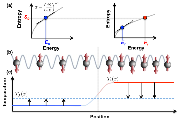
Figure 1: a) If the Hamiltonian in the “bath” region is related to the Hamiltonian in the “system” region by a constant rescaling, $H_{B}=\lambda H_{S}$, their entropy-energy-density curves satisfy $s_{B}(E)=s_{S}(E/\lambda)$. Thus preparing at state with constant entropy density establishes a temperature differential $T_{B}=\lambda T_{S}$, since $T=\frac{dE}{dS}$. b) Schematic representation of particles or spins interacting through a long-range, power-law interaction $1/R^{\alpha}$. If the interparticle spacing on the left (“bath”) is increased by a factor $d$ relative to the right (“system”), then $H_{B}=(\frac{1}{d})^{\alpha}H_{S}$ Moses et al. (2015). c) In this case, a uniform Neél state has a temperature differential after reaching local equilibrium, and the resulting evolution will remove entropy from the right half of the chain as the system reaches global equilibrium.

In this work, we propose and analyze a class of methods—termed ‘conformal cooling quenches’—for shifting entropy by spatially modulating the magnitude of the Hamiltonian mag . The intuition behind this approach is best illustrated as follows: Suppose that we take a system’s Hamiltonian $H$ and either suddenly or adiabatically reduce it by a factor $\lambda<1$, taking $H\to\lambda H$. Since $k_{B}T$ has units of energy, the temperature $T$ is accordingly reduced by $T\to\lambda T$. When applied to the entire system, this “cooling” is trivial, since it amounts to a change of units without reducing the entropy density. However, if the reduction by $\lambda$ instead occurs for only a portion of the system, which we call the ‘bath,’ the change in temperature is physical, and establishes a temperature gradient; during equilibration, entropy will then flow out of the system and into the bath.

This generalizes previous studies, where entropy flow relies on particle itinerance, while the temperature gradient is inherited from a density gradient Mazurenko et al. (2017); Kantian et al. (2018); Chiu et al. (2018). In particular, our method is applicable not only to itinerant Hubbard systems, but also to spin models. This latter case is especially relevant to recent developments in trapped ion arrays Britton et al. (2012); Zhang et al. (2017), optical tweezer arrays Labuhn et al. (2016); Bernien et al. (2017), and ultracold molecules Yan et al. (2013a); Anderegg et al. (2019), where versatile spin models with spatially tunable Hamiltonian parameters are increasingly accessible.

One virtue of the conformal cooling approach is that it can “cool” a system within a metastable state-space. For example, conformal cooling can be applied to a gas equilibrating at negative kinetic or spin temperature Braun et al. (2013), bringing the system toward zero temperature from below. It can also be applied to gases equilibrating in high-energy manifolds of states, i.e. in excited bands of an optical lattice Müller et al. (2007); Wirth et al. (2011). Systems equilibrating at negative temperatures or in higher bands can exhibit strong frustration without complicated band engineering.

We will begin by introducing the thermodynamics of our approach, focusing on two questions: 1) how much entropy can a cooling quench remove and 2) how long does it take? Next, we perform a large-scale numerical study of both a 1D topological spin-chain and the fermionic Hubbard model, demonstrating that realistic cooling quenches can remove enough entropy to reveal their low-temperature physics. Finally, we discuss natural experimental implementations of our approach focusing on ultracold polar molecules and Rydberg atom arrays.

General Strategy—We envision spatially demarcating the degrees of freedom into a “bath” (B) and “system” (S) which are placed “end-to-end,” so that the coupling between their boundaries scales sub-extensively with their volume (Fig. 1b) sid . We assume that the Hamiltonian $H_{B}$ (bath) is identical to $H_{S}$ (system), except that its magnitude is scaled by a factor $\lambda<1$. The entropy ($s$) versus energy density ($E$) curves in the two regions are then related by $s_{B}(E)=s_{S}(E/\lambda)$ and their temperatures by $T_{B}(E)=\lambda T_{S}(E/\lambda)$ (Fig. 1a). In the following, we will consider two protocols, “quenched” and “adiabatic.”

Quench Protocol—In the quench approach, the Hamiltonians are time-independent with $H_{B}=\lambda H_{S}$. At $t=0$, we prepare a uniform initial state (e.g. a product state) and simply let it evolve. Equivalently, one can begin in thermal equilibrium with $H_{B}=H_{S}$, and then suddenly reduce $H_{B}$ to $H_{B}=\lambda H_{S}$. The overall system is now in local equilibrium, with the local density matrices in $B$ and $S$ identical, and thus, $s_{B}=s_{S}$ and $T_{B}=\lambda T_{S}$. As the system evolves toward global equilibrium, entropy will follow the thermal gradient and flow from $S$ to $B$.

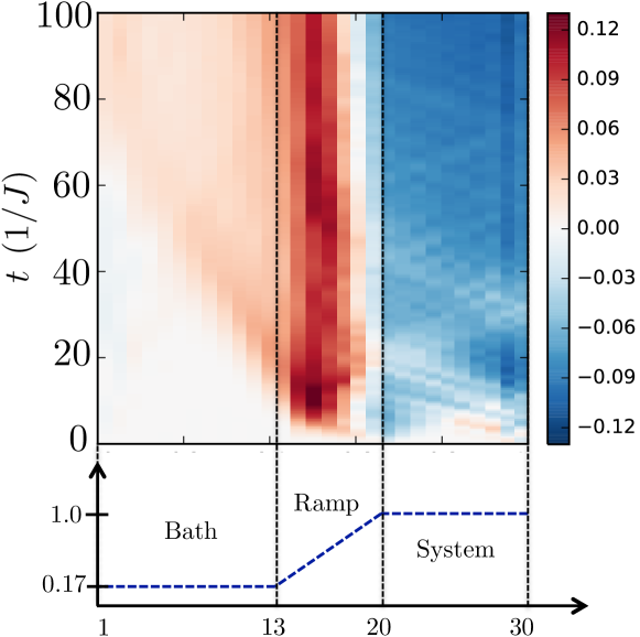
Figure 2: ‘Quench’ cooling of a 30-site spin-1 Haldane chain. After initializing the state at $t=0$ with uniform entropy density, the coupling constants $\lambda_{x}$ are scaled according to the bottom panel, which should transport heat from the ‘system’ on the right to the ‘bath’ on the left. In the top panel, we plot the change in energy density $h_{x}(t)-h_{x}(0)$ as the chain evolves.

The final equilibrium temperature $T_{\textrm{f}}^{(q)}$ is determined by energy conservation post-quench. Noting that the energy just after the quench is $N_{S}E_{S}(T_{i})+N_{B}\lambda E_{S}(T_{i})$, and using the relation $E_{B}(T)=\lambda E_{S}(T/\lambda)$, we have:

$$(N_{S}+\lambda N_{B})E_{S}(T_{\textrm{i}})=N_{S}E_{S}(T_{\textrm{f}}^{(q)})+N_{B}\lambda E_{S}(T_{\textrm{f}}^{(q)}/\lambda),$$ (1)

where $N_{S},N_{B}$ are the number of sites in the system and bath, and $T_{\textrm{i}}$ is the initial temperature of the system. When $\lambda N_{B}\gg N_{S}$, we have $T_{\textrm{f}}^{(q)}=\lambda T_{i}$, but more generally one should choose $\lambda$ so as to minimize $T_{\textrm{f}}^{(q)}$ based on the precise form of $E_{S}(T)$. While we have assumed a sharp distinction between $S$ and $B$ for simplicity, one can let the spatial modulation $\lambda(\vec{x})$ vary smoothly, for example in the “ramp” region shown in Figs. 2 and 4(a), in which case Eq. (1) is replaced by an integral over the energy density.

Adiabatic Protocol—The cooling is more effective if the magnitude of $H_{B}=\Lambda(t)H_{S}$ is instead slowly reduced in time, with $\Lambda(t=0)=1$ and $\Lambda(t\rightarrow\infty)=\lambda$. In the isentropic limit, the final system temperature $T_{\textrm{f}}^{(a)}$ is determined by

$$(N_{B}+N_{S})s_{S}(T_{\textrm{i}})=N_{B}s_{S}(T_{\textrm{f}}^{(a)}/\lambda)+N_{S}s_{S}(T_{\textrm{f}}^{(a)}),$$ (2)

with $T_{\textrm{f}}^{(a)}\leq T_{\textrm{f}}^{(q)}$. When the bath and system are end-to-end, diffusive dynamics imply that the equilibration time, $t_{\textrm{eq}}$, scales as $L_{S}^{2}/\Lambda(t)$ (q.v. Eq. (4)) where $L_{S}$ is the linear extent of the system and adiabaticity requires $\partial_{t}\Lambda\ll 1/t_{\textrm{eq}}$. For small $\Lambda$, the bath and system will eventually fall out of equilibrium and additional entropy will be produced, though the temperature will always be upper-bounded by $T_{\textrm{f}}^{(q)}$.

To demonstrate that conformal cooling can shift significant entropy out of the system even for moderate bath sizes and short time-scales, we numerically investigate two distinct settings: the $S=1$ Haldane topological anti-ferromagnet and the fermionic Hubbard model.

Conformal cooling in an $S=1$ Haldane chain—Consider a one dimensional chain of $S=1$ spins with Hamiltonian

$$H[\lambda_{x}]=\sum_{x}\lambda_{x}h_{x}=J\sum_{x}\lambda_{x}\left[\mathbf{S}_{x}\cdot\mathbf{S}_{x+1}+\frac{\gamma}{3}(\mathbf{S}_{x}\cdot\mathbf{S}_{x+1})^{2}\right].$$ (3)

At both the Heisenberg point $\gamma=0$ and the AKLT point $\gamma=1$, the spin-chain is a gapped topological paramagnet in the Haldane phase Haldane (1983); Affleck et al. (1987). The topology of the phase has a striking signature in a finite-length chain, which exhibits a pair of localized spin-1/2 edge states. At temperatures below the bulk gap, $T<\Delta\sim J$, these localized edge states can coherently store quantum information for long times, providing a sharp experimental signature of the topological phase Senko et al. (2015).

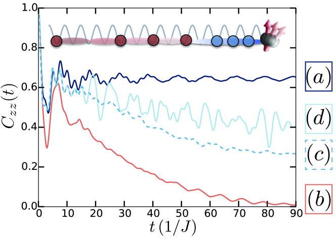
Figure 3: The dynamical correlation function, $C_{zz}(t)$, measured after four initialization protocols: a) Optimal: $C_{zz}(t)$ for the ground state of an $L=10$ chain; b) finite $T=0.51J$, without a cooling quench. The edge coherence rapidly decays. c) finite $T_{i}=0.51J$, but starting the $C_{zz}$ measurement after the cooling quench shown in Fig. 2. The coherence is improved by an order of magnitude. d) Same as (c), but eliminating the coupling between sites $i=20$ and $21$ after the quench, which cuts off the bath.

Calculating the thermodynamic energy-temperature relation, $E(T)$, using exact diagonalization reveals that a modest bath size of $N_{B}/N_{S}\approx$ 2-3 is sufficient to cool from the Neél product state $\ket{\uparrow\downarrow\uparrow\downarrow\cdots}$, which corresponds to an initial temperature $T_{\textrm{i}}=1.45\Delta$, to well below the gap, $T_{\textrm{f}}^{(q)}\approx 0.7\Delta$ sup . Here the pure-state temperature is defined by inverting $E(T)$. Since the spin chain is diffusive Damle and Sachdev (1998), the time-scale required for cooling is determined by Fourier’s law. When $\lambda(x)$ varies smoothly compared to the lattice scale, the local thermal conductivity $\kappa$ and specific heat $c$ are determined by rescaling, $\kappa(T,x)=\lambda(x)\kappa_{S}(T(x)/\lambda(x))$ and $c(T,x)=c_{S}(T(x)/\lambda(x))$, where $\kappa_{S}(T)$ and $c_{S}(T)$ are defined with $\lambda=1$. Applying this within a simple lumped element model predicts that temperature will decrease as sup ,

$$T_{S}(t)\sim T_{\textrm{f}}^{(q)}+\mathcal{K}\frac{L_{S}}{\sqrt{tD_{B}}}(T_{\textrm{i}}-T_{\textrm{f}}^{(q)})$$ (4)

where $D_{B}$ is the thermal diffusivity of the bath and $\mathcal{K}$ is an $\mathcal{O}(1)$ geometrical factor. For bath temperatures above $\lambda J$, the diffusivity will generically saturate to a temperature-independent value, $D_{B}\propto\lambda J/\hbar$ Karadamoglou and Zotos (2004), implying that $t_{\textrm{eq}}\sim L_{S}^{2}(\lambda J/\hbar)^{-1}$.

To verify these dynamics, we simulate the evolution of a finite-energy density pure state using the TEBD-algorithm Vidal (2003). It is exponentially difficult to simulate finite temperature dynamics, limiting our system to $L=30$ sites (Fig. 2) gam . We initialize a uniform state $\ket{\Psi(0)}=e^{-\tau\hat{H}[\lambda_{x}=1]}\ket{\uparrow\downarrow\uparrow\downarrow\cdots}$, where $\tau=0.35/J$, resulting in an energy density that corresponds to temperature $T_{S}=0.51J$ after local equilibration con . The system is then quenched into a spatially non-uniform $\hat{H}[\lambda_{x}]$ (Fig. 2). Using the optimal $\lambda_{0}=0.17$ in the ‘bath’ leads to a final predicted temperature: $T_{\textrm{f}}^{(q)}=0.29J$.

The evolution of the local energy density $\langle\lambda_{x}\hat{h}_{x}(t)\rangle$ during the cooling quench is depicted in Fig. 2. The energy density in region $S$ at time $t=100/J$ corresponds to $T_{S}=0.34J$, within $14\%$ of the expected $T_{\textrm{f}}^{(q)}$ sup . Moreover, the relaxation dynamics are roughly consistent with $T_{S}\sim T_{\textrm{f}}^{(q)}+(T_{\textrm{i}}-T_{\textrm{f}}^{(q)})\sqrt{t_{\textrm{eq}}/t}$, where $t_{\textrm{eq}}\approx 0.22(\mathcal{K}L_{S})^{2}(\lambda J/\hbar)^{-1}$, consistent with the expectation $1/D_{B}\sim 0.19/\lambda$ Karadamoglou and Zotos (2004); sup .

Even for a relatively small bath size, the cooling quench has a dramatic effect on the dynamical correlation function of the topological edge mode. Since the edge state in region $S$ will generically have overlap with the right-most spin $S^{\mu}_{\textrm{end}}$, its coherence can be probed via the correlation function

$$C_{zz}(t)=\bra{\Psi}S_{\textrm{end}}^{z}(t+t_{f})S_{\textrm{end}}^{z}(t_{f})\ket{\Psi},$$ (5)

where the measurement only begins after the cooling quench is complete ($t_{f}=100/J$). At $T=0$, these correlations should asymptote to a finite constant [Fig. 3a], while at large $T$ [Fig. 3d], they will decay exponentially. We compare $C_{zz}(t)$ under four preparation scenarios described in Fig. 3. The conformal cooling quench improves the coherence time (i.e. the decay timescale of $C_{zz}(t)$) by more than an order of magnitude.

Adiabatic conformal cooling in the fermionic Hubbard model—We next consider the adiabatic protocol applied to the fermionic Hubbard model, $H=-\sum_{<i,j>,\sigma}t_{ij}c^{\dagger}_{i\sigma}c_{j\sigma}+U\sum_{i}n_{i\uparrow}n_{i\downarrow}-\mu\sum_{i\sigma}n_{i\sigma}$. Here, we focus on the Mott insulating phase at half-filling with $t/U\ll 1$ and $T<U$. While the fermions’ motion is quenched, their spins interact via an effective anti-ferromagnetic Heisenberg interaction, $H_{\textrm{eff}}=\sum_{\left<i,j\right>}J_{ij}[\mathbf{S}_{i}\cdot\mathbf{S}_{j}-\frac{1}{4}]$, where $J=4\frac{t_{ij}^{2}}{U}$ is the super-exchange coupling.

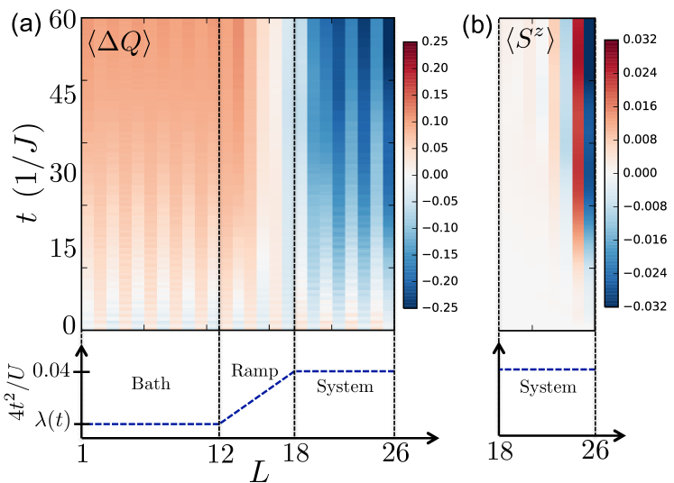
Figure 4: Cooling dynamics in the 1D spinful Hubbard model. a) After initializing a $T=1.4J$ thermal state with uniform Hamiltonian $U=1,t_{ij}=0.1$, the hopping $t_{ij}$ is adiabatically decreased with a spatial profile shown in the bottom panel. The top panel shows the change in the heat density as a function of time. b) Depicts the onset of antiferromagnetic correlations. The right-most site has a small Zeeman field $0.05S^{z}$. While the initial temperature disorders the spins, as the system cools, algebraic anti-ferromagnetic correlations clearly emerge.

In the Mott regime where the dynamics are governed by $H_{\textrm{eff}}$, adiabatic cooling is naturally realized by decreasing $J$ in the bath region (relative to the system region); one can achieve this by weakly modulating the depth of the optical potential, $V(\vec{x})=-V_{0}(\vec{x})\sum_{i=1}^{d}\cos(k\,x^{i})^{2}$, where $V_{0}(\vec{x})$ is slowly varying and $k$ is the wavevector of optical lattice. Increasing $V_{0}$ has three effects on the effective Hamiltonian: $U$ will increase, as the orbitals are further localized, $\mu$ will increase, as the trap is deeper and $t$ will decrease due to the barrier height. Since $t$ is exponentially more sensitive than $U$ to the trap-depth, $\xi=\sqrt{\frac{V_{0}}{E_{r}}}$ ($E_{r}$ is the recoil energy), the dominant effect is to modulate the hoppings Hofstetter et al. (2002). Assuming $\mu$ is compensated to maintain half-filling, the super-exchange energy becomes $J_{ij}\propto\xi^{2}(x)e^{-4\xi(x)}$, precisely the desired modulation. Fortuitously, a small modulation in $V_{0}$ is already capable of dramatically reducing the system’s temperature; for example, in the the 3D cubic Heisenberg model, a $6\%$ change in the lattice depth can cool the system from $1.4T_{\textrm{N}}$ Hart et al. (2015) down to the Néel temperature, $T_{\textrm{N}}$ sup .

Note that in the above approach, we choose to scale $t$ but not $U$, which differs from the overall scaling, $H\to\lambda H$, we had initially used to motivate our work. Of course in the limit $t,T\ll U$, the conclusions are the same because the thermodynamics are governed by $H_{\textrm{eff}}\propto J=4t^{2}/U$, so scaling $t$ does effectively enact an overall scaling of the Hamiltonian. But more generally, cooling only requires the criteria $\partial_{t}T(s;t,U)>0$, which we have verified using determinantal quantum Monte Carlo sup , so long as the initial entropy density satisfies $s<k_{B}\log(2)$ Daré et al. (2007). To this end, our proposal will also work away from the $t,T\ll U$ limit.

To confirm the effectiveness of the adiabatic protocol, we simulate the dynamics of the spinful 1D fermionic Hubbard model. We use the TEBD method to time evolve a purified finite-temperature ensemble Karrasch et al. (2013). At time $t=0$ the Hamiltonian is uniform, $U=1,t_{ij}=0.1$, with an initial thermal state $\rho=e^{-H/T_{i}}/\mathcal{Z}$ at $T_{i}=1.4J$. We then time evolve the ensemble with a Hamiltonian, $H(t)$, in which $t_{ij}$ decreases adiabatically in the bath sup . Since Hamiltonian changes in time, energy is not conserved, and we divide it into heat and work, $\dot{E}=\dot{Q}-\dot{W}$ sup , enabling us to plot the evolution of the heat-density $Q$ in Fig. 4(a). Total heat is conserved, but with clear transport from $S$ to $B$. As a more qualitative thermometer, we note that at $T=0$, the system should display algebraic anti-ferromagnetic correlations. To reveal them, we place a small Zeeman field $H=0.05S^{z}$ on the right edge spin, both in the initial thermal state and the subsequent dynamics. As depicted in Fig. 4(b), the finite temperature of the initial thermal state disorders the magnetization $\langle S^{z}\rangle$, but as the dynamics proceed and cooling occurs, the antiferromagnetic correlations become clearly manifest.

Experimental implementation—Our conformal cooling protocols are well suited to systems with long-ranged interactions, such as polar molecules, Rydberg atoms, and trapped ions Yan et al. (2013b); Moses et al. (2015); Zeiher et al. (2016); Smith et al. (2015); Martinez et al. (2016). To implement the quench protocol, we envision a setup where the average spacing between particles is larger in the bath than in the system, $r_{B}>r_{S}$. Assuming power-law interactions ($1/R^{\alpha}$), the Hamiltonian in $B$ will be reduced by a constant factor $\lambda=(r_{S}/r_{B})^{\alpha}$ relative to that in $S$ (Fig. 1b) lon .

This approach is particularly applicable to two classes of current generation experimental platforms: ultracold polar molecules and Rydberg atom arrays. In the molecular context, the optical lattice filling fraction, $\nu<1$, leads to random dilution Moses et al. (2015). Fortunately, the cooling quench is natural to implement in this randomly diluted case, since one can make $r_{B}>r_{S}$ merely by modulating the average density, without having to ensure the particles in $B$ lie on a particular sub-lattice. In this case, simply time-evolving an initial product state in the presence of this density modulation will cool the high-density region, and could provide a simple route towards studying, for example, algebraically correlated random-singlet phases Gorshkov et al. (2011); Yao et al. (2015); Fisher (1994).

Although we have studied the AKLT model because it admits simple numerical observables for quantifying entropy, the same cooling protocol can also be applied to the long-range, mixed-field Ising model, which is naturally realized in a Rydberg atom array Labuhn et al. (2016); Bernien et al. (2017); Keesling et al. (2019); de Léséleuc et al. (2019); Browaeys and Lahaye (2020). In this case, the spacing between the atoms and/or the intensity of the Rydberg excitation light, can be made spatially varying, in order to create well-defined bath and system regions in one, two, or even three-dimensions Endres et al. (2016); Barredo et al. (2016, 2018). The complex phase diagram associated with this model exhibits a variety of competing orders and phase transitions, providing a rich playground for implementing conformal cooling Samajdar et al. (2020).

In summary, we have proposed a general method for preparing low-entropy many-body states in isolated quantum systems. Our approach can be naturally implemented in systems with power law interactions by simply diluting the particle density of the bath region; moreover, in the supplemental materials, we also provide a simple experimental blueprint for implementing conformal cooling in the spinful fermionic Hubbard model sup . Looking forward, our proposal raises a number of intriguing questions: is it possible to implement a refrigeration cycle by repeated preparation of the bath state? Can one optimize a side-by-side geometry which could reduce the equilibration time? By performing conformal cooling during a quantum phase transition, can one reduce the rate of Kibble-Zurek defect formation Keesling et al. (2019)?