How to scale distributed deep learning?

Abstract

Training time on large datasets for deep neural networks is the principal workflow bottleneck in a number of important applications of deep learning, such as object classification and detection in automatic driver assistance systems (ADAS). To minimize training time, the training of a deep neural network must be scaled beyond a single machine to as many machines as possible by distributing the optimization method used for training. While a number of approaches have been proposed for distributed stochastic gradient descent (SGD), at the current time synchronous approaches to distributed SGD appear to be showing the greatest performance at large scale. Synchronous scaling of SGD suffers from the need to synchronize all processors on each gradient step and is not resilient in the face of failing or lagging processors. In asynchronous approaches using parameter servers, training is slowed by contention to the parameter server. In this paper we compare the convergence of synchronous and asynchronous SGD for training a modern ResNet network architecture on the ImageNet classification problem. We also propose an asynchronous method, gossiping SGD, that aims to retain the positive features of both systems by replacing the all-reduce collective operation of synchronous training with a gossip aggregation algorithm. We find, perhaps counterintuitively, that asynchronous SGD, including both elastic averaging and gossiping, converges faster at fewer nodes (up to about 32 nodes), whereas synchronous SGD scales better to more nodes (up to about 100 nodes).

1 Introduction

Estimates of the data gathered by a self-driving car start from at least 750 MB/s. With proper annotation or through an unsupervised learning scheme, all of this data can become useful for training the object detection system or grid-occupancy system of a self-driving car. The resulting training set can lead to weeks or more of training time on a single CPU/GPU system. Therefore, for such applications training time defines the most time consuming element of the workflow, and reduced training time is highly desirable.

To achieve significant reductions in training time, the training must be distributed across multiple CPUs/GPUs with the goal of strong scaling: as more nodes are thrown at the problem, the training time should ideally decrease proportionally. There are two primary approaches to distributed stochastic gradient descent (SGD) for training deep neural networks: (i) synchronous all-reduce SGD based on a fast all-reduce collective communication operation [1, 2, 3, 4], and (ii) asynchronous SGD using a parameter server [5, 6].

Both approaches (i) and (ii) have weaknesses at scale. Synchronous SGD is penalized by straggling processors, underutilizes compute resources, and is not robust in the face of failing processors or nodes. On the other hand, asynchronous approaches using parameter servers create a communication bottleneck and underutilize the available network resources, slowing convergence.

Individual researchers also have different numbers of nodes at their disposal, including compute and network resources. So determining the best approach for a given number of nodes, as well as the approach that scales to the most number of nodes, is of interest to practitioners with finite resources.

We are concerned with the following questions:

1. How fast do asynchronous and synchronous SGD algorithms converge at both the beginning of training (large step sizes) and at the end of training (large step sizes)?

2. How does the convergence of async. and sync. SGD vary with the number of nodes?

To compare the strengths and weaknesses of asynchronous and synchronous SGD algorithms, we train a modern ResNet convolutional network [7] on the ImageNet dataset [8] using various distributed SGD methods. We primarily compare synchronous all-reduce SGD, the recently proposed asynchronous elastic averaging SGD [9], as well as our own method, asynchronous gossiping SGD, based on an algorithm originally developed in a different problem setting [10]. Gossiping SGD is an asynchronous method that does not use a centralized parameter server, and in a sense, gossiping is a decentralized version of elastic averaging. We find that asynchronous SGD, including both elastic averaging and gossiping, exhibits the best scaling at larger step sizes and, perhaps counterintuitively, at smaller scales (up to around 32 distributed nodes). For smaller step sizes and at larger scales, all-reduce consistently converges to the most accurate solution faster than the asynchronous methods.

2 Background

In this section, we will describe the baseline synchronous and asynchronous SGD methods, as well as a recently proposed asynchronous method that is more scalable than its predecessor. We will use the following naming convention for SGD: $\theta$ are the parameters over which the objective is minimized, $\tilde{\theta}$ is the center parameter (if applicable), $\alpha$ is the step size, $\mu$ is the momentum, subscript $i$ refers to the $i$-th node out of $p$ total nodes, and subscript $t$ refers to the $t$-th (minibatch) iteration. Additionally, $b$ will refer to the per-node minibatch size, whereas $m$ will refer to the aggregate minibatch size summed across all nodes.

2.1 Synchronous All-Reduce SGD

In traditional synchronous all-reduce SGD, there are two alternating phases proceeding in lock-step: (1) each node computes its local parameter gradients, and (2) all nodes collectively communicate all-to-all to compute an aggregate gradient, as if they all formed a large distributed minibatch. The second phase of exchanging gradients forms a barrier and is the communication-intensive phase, usually implemented by an eponymous all-reduce operation. The time complexity of an all-reduction can be decomposed into latency-bound and bandwidth-bound terms. Although the latency term scales with $O(\log(p))$, there are fast ring algorithms which have bandwidth term independent of $p$ [11]. With modern networks capable of handling bandwidth on the order of 1–10 GB/s combined with neural network parameter sizes on the order of 10–100 MB, the communication of gradients or parameters between nodes across a network can be very fast. Instead, the communication overhead of all-reduce results from its use of a synchronization barrier, where all nodes must wait for all other nodes until the all-reduce is complete before proceeding to the next stochastic gradient iteration. This directly leads to a straggler effect where the slowest nodes will prevent the rest of the nodes from making progress. Examples of large-scale synchronous data parallel SGD for distributed deep learning are given in [1], [2], [3], and [4]. We provide pseudocode for synchronous data-parallel SGD in Algorithm 1.

Algorithm 1 Synchronous all-reduce SGD.

  initialize $\theta_{0,i}\leftarrow\theta_{0}$

  for $t\in\{0,\ldots,T\}$ do

     $\Delta\theta_{t,i}\leftarrow-\alpha_{t}\nabla f_{i}(\theta_{t,i};X_{t,i})+\mu\Delta\theta_{t-1}$

     $\Delta\theta_{t}\leftarrow\text{all-reduce-average}(\Delta\theta_{t,i})$

     $\theta_{t+1,i}\leftarrow\theta_{t,i}+\Delta\theta_{t}$

  end for

2.2 Asynchronous Parameter-Server SGD

A different approach to SGD consists of each node asynchronously performing its own gradient updates and occasionally synchronizing its parameters with a central parameter store. This form of asynchronous SGD was popularized by “Hogwild” SGD [12], which considered solving sparse problems on single machine shared memory systems. “Downpour” SGD [5] then generalized the approach to distributed SGD where nodes communicate their gradients with a central parameter server. The main weakness of the asynchronous parameter-server approach to SGD is that the workers communicate all-to-one with a central server, and the communication throughput is limited by the finite link reception bandwidth at the server. One approach for alleviating the communication bottleneck is introducing a delay between rounds of communication, but increasing the delay greatly decreases the rate of convergence [9]. Large scale asynchronous SGD for deep learning was first implemented in Google DistBelief [5] and has also been implemented in [6]; large scale parameter server systems in the non-deep learning setting have also been demonstrated in [13] and [14].

2.3 Elastic Averaging SGD

Elastic averaging SGD [9] is a new algorithm belonging to the family of asynchronous parameter-server methods which introduces a modification to the usual stochastic gradient objective to achieve faster convergence. Elastic averaging seeks to maximize the consensus between the center parameter $\tilde{\theta}$ and the local parameters $\theta_{i}$ in addition to the loss:

$$F_{\text{consensus}}(\theta_{1},\ldots,\theta_{p},\tilde{\theta}) =\sum_{i=1}^{p}\left[f(\theta_{i};X_{i})+\frac{\rho}{2}\|\theta_{i}-\tilde{\theta}\|^{2}\right].$$ (1)

The elastic averaging algorithm is given in Algorithm 2. The consensus objective of elastic averaging is closely related to the augmented Lagrangian of ADMM, and the gradient update derived from the consensus objective was shown by [9] to converge significantly faster than vanilla async SGD. However, as elastic averaging is a member of the family of asynchronous parameter-server approaches, it is still subject to a communication bottleneck between the central server and the client workers.

Because recent published results indicate that elastic averaging dominates previous asynchronous parameter-server methods [9], we will only consider elastic averaging from this point on.

Algorithm 2 Elastic averaging SGD. The hyperparameter $\beta$ is the moving rate.

  # client code

  initialize $\theta_{0,i}\leftarrow\theta_{0}$

  for $t\in\{0,\ldots,T\}$ do

     if $t>0$ and $t\equiv 0\mod\tau$ then

        $\tilde{\theta}\leftarrow\text{receive-server-param}()$

        $\text{send-param-update}(+\beta(\theta_{t,i}-\tilde{\theta}))$

        $\theta_{t,i}\leftarrow\theta_{t,i}-\beta(\theta_{t,i}-\tilde{\theta})$

     end if

     $\Delta\theta_{t,i}\leftarrow-\alpha_{t}\nabla f_{i}(\theta_{t,i};X_{t,i})+\mu\Delta\theta_{t-1,i}$

     $\theta_{t+1,i}\leftarrow\theta_{t,i}+\Delta\theta_{t,i}$

  end for

  # server code

  initialize $\tilde{\theta}_{0}\leftarrow\theta_{0}$

  for $t\in\{0,\ldots,T\}$ do

     $\text{send-server-param}(\tilde{\theta}_{t})$

     $\Delta\theta\leftarrow\text{receive-param-update}()$

     $\tilde{\theta}_{t+1}\leftarrow\tilde{\theta}_{t}+\Delta\theta$

  end for

3 Gossiping SGD

3.1 Algorithm

In a nutshell, the synchronous all-reduce algorithm consists of two repeating phases: (1) calculation of the local gradients at each node, and (2) exact aggregation of the local gradients via all-reduce. To derive gossiping SGD, we would like to replace the synchronous all-reduce operation with a more asynchronous-friendly communication pattern. The fundamental building block we use is a gossip aggregation algorithm [15, 16], which combined with SGD leads to the gossiping SGD algorithm. Asynchronous gossiping SGD was introduced in [10] for the general case of a sparse communication graph between nodes (e.g. wireless sensor networks). The original problem setting of gossiping also typically involved synchronous rounds of communication, whereas we are most interested in asynchronous gossip.

The mathematical formulation of the gossiping SGD update can also be derived by conceptually linking gossiping to elastic averaging. Introduce a distributed version of the global consensus objective, in which the center parameter is replaced with the average of the local parameters:

$$F_{\text{dist-consensus}}(\theta_{1},\ldots,\theta_{p}) =\sum_{i=1}^{p}\left[f(\theta_{i};X_{i})+\frac{\rho}{2}\left\|\theta_{i}-\frac{1}{p}\sum_{j=1}^{p}\theta_{j}\right\|^{2}\right].$$ (2)

The corresponding gradient steps look like the following:

$$\theta_{t,i}^{\prime} =\theta_{t,i}-\alpha\nabla f(\theta_{t,i};X_{i})$$ (3)

$$\theta_{t+1,i} =\theta_{t,i}^{\prime}-\beta\left(\theta_{t,i}^{\prime}-\frac{1}{p}\sum_{j=1}^{p}\theta_{t,j}^{\prime}\right).$$ (4)

If we replace the distributed mean $\frac{1}{p}\sum_{j=1}^{p}\theta_{t,j}$ with the unbiased one-node estimator $\theta_{t,j_{t,i}}$, such that $j_{t,i}\sim\text{Uniform}(\{1,\ldots,p\})$ and $\mathbb{E}[\theta_{t,j_{t,i}}]=\frac{1}{p}\sum_{j=1}^{p}\theta_{t,j}$, then we derive the gossiping SGD update:

$$\theta_{t,i}^{\prime} =\theta_{t,i}-\alpha\nabla f(\theta_{t,i};X_{i})$$ (5)

$$\theta_{t+1,i} =\theta_{t,i}^{\prime}-\beta(\theta_{t,i}^{\prime}-\theta_{j_{t,i},t}^{\prime})$$ (6)

$$=(1-\beta)\theta_{t,i}^{\prime}+\beta\theta_{j_{t,i},t}^{\prime}.$$ (7)

To make this more intuitive, we describe a quantity related to the distributed consensus, the diffusion potential. Fix $\theta_{i}^{(0)}=\theta_{t,i}$, and consider the synchronous gossip setting of purely calculating an average of the parameters and where there are no gradient steps. Then the updated parameter after $k$ repeated gossip rounds, $\theta_{i}^{(k)}$, can be represented as a weighted average of the initial parameter values $\theta_{j}^{(0)}$. Denoting the weighted contribution of $\theta_{j}^{(0)}$ toward $\theta_{i}^{(k)}$ by $v_{i,j}^{(k)}$, the diffusion potential is:

$$\Phi_{\text{diffusion}}(\theta_{1}^{(k)},\ldots,\theta_{p}^{(k)}) =\sum_{i=1}^{p}\sum_{j=1}^{p}\left\|v_{i,j}^{(k)}\theta_{j}^{(0)}-\frac{1}{p}\sum_{j^{\prime}=1}^{p}v_{i,j^{\prime}}^{(k)}\theta_{j^{\prime}}^{(0)}\right\|^{2}.$$ (8)

It can be shown that repeated rounds of a form of gossiping reduces the diffusion potential by a fixed rate per round [15].

If $j_{t,i}$ is chosen uniformly as above, then the algorithm is equivalent to “pull-gossip,” i.e. each node pulls or receives $\theta_{j}$ from one and only one other random node per iteration. On the other hand, if we replace the “one-node estimator” with querying $\theta_{j}$ from multiple nodes, with the constraint that each $j$ is represented only once per iteration, then the algorithm becomes “push-gossip,” i.e. each node pushes or sends its own $\theta_{i}$ to one and only one other random node, while receiving from between zero and multiple other nodes. Push-gossiping SGD can be interpreted as an interleaving of a gradient step and a simplified push-sum gossip step [15]. Algorithms 3 and 4 describe pull-gossiping and push-gossiping SGD respectively.

Algorithm 3 Pull-gossiping SGD.

  initialize $\theta_{0,i}\leftarrow\theta_{0}$

  for $t\in\{0,\ldots,T\}$ do

     if $t>0$ and $t\equiv 0\mod\tau$ then

        set $x_{i}\leftarrow\theta_{t,i}$

        choose a target $j$

        $\theta_{t,i}\leftarrow$ average of $x_{i},x_{j}$

     end if

     $\Delta\theta_{t,i}\leftarrow-\alpha_{t}\nabla f_{i}(\theta_{t,i};X_{t,i})+\mu\Delta\theta_{t-1,i}$

     $\theta_{t+1,i}\leftarrow\theta_{t,i}+\Delta\theta_{t,i}$

  end for

Algorithm 4 Push-gossiping SGD.

  initialize $\theta_{0,i}\leftarrow\theta_{0}$

  for $t\in\{0,\ldots,T\}$ do

     if $t>0$ and $t\equiv 0\mod\tau$ then

        set $x_{i}\leftarrow\theta_{t,i}$

        choose a target $j$

        send $x_{i}$ to $i$ (ourselves) and to $j$

        $\theta_{t,i}\leftarrow$ average of received $x$’s

     end if

     $\Delta\theta_{t,i}\leftarrow-\alpha_{t}\nabla f_{i}(\theta_{t,i};X_{t,i})+\mu\Delta\theta_{t-1,i}$

     $\theta_{t+1,i}\leftarrow\theta_{t,i}+\Delta\theta_{t,i}$

  end for

3.2 Analysis

Our analysis of gossiping SGD is based on the analyses in [17, 16, 10, 18, 9]. We assume that all processors are able to communicate with all other processors at each step. The main convergence result is the following:

Theorem 1.

Let $f$ be a $m$-strongly convex function with $L$-Lipschitz gradients. Assume that we can sample gradients $g=\nabla f(\theta;X_{i})+\xi_{i}$ with additive noise with zero mean $\mathbb{E}[\xi_{i}]=0$ and bounded variance $\mathbb{E}[\xi_{i}^{T}\xi_{i}]\leq\sigma^{2}$. Then, running the asynchronous pull-gossip algorithm, with constant step size $0<\alpha\leq\tfrac{2}{m+L}$, the expected sum of squares convergence of the local parameters to the optimal $\theta_{\ast}$ is bounded by

$$\mathbb{E}[\|\theta_{t}-\theta_{\ast}\mathbf{1}\|^{2}]\leq\left(1-\frac{2\alpha}{p}\frac{mL}{m+L}\right)^{t}\|\theta_{0}-\theta_{\ast}\mathbf{1}\|^{2}+p\alpha\sigma^{2}\frac{m+L}{2mL}$$ (9)

Furthermore, with the additional assumption that the gradients are uniformly bounded as $\sup|\nabla f(\theta)|\leq C$, the expected sum of squares convergence of the local parameters to the mean $\bar{\theta}_{t}$ is bounded by

$$\mathbb{E}[\|\theta_{t}-\bar{\theta}_{t}\mathbf{1}\|^{2}] \leq\left(\lambda\left(1-\frac{\alpha\,m}{p}\right)\right)^{t}\|\theta_{0}-\bar{\theta}_{0}\mathbf{1}\|^{2}+\frac{\lambda\alpha^{2}(C^{2}+\sigma^{2})}{1-\lambda\left(1-\frac{\alpha\,m}{p}\right)}$$ (10)

$$\text{ where }\lambda =1-\frac{2\beta(1-\beta)}{p}-\frac{2\beta^{2}}{p}$$ (11)

For the proofs, please see subsection (6.1) in the supplementary material.

4 Experiments

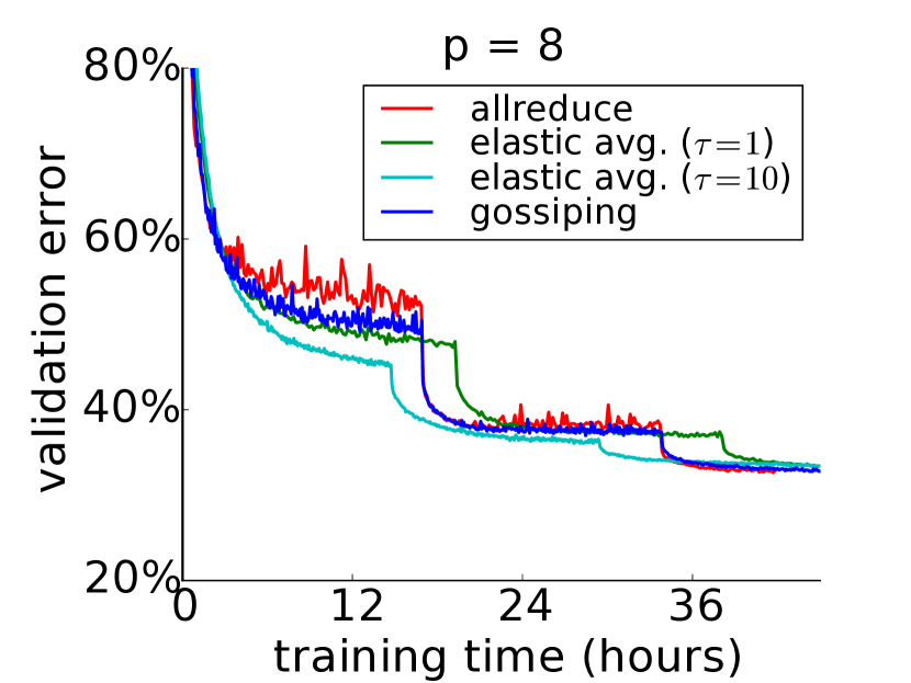
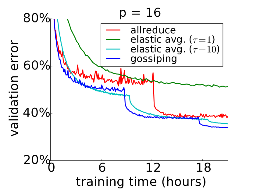
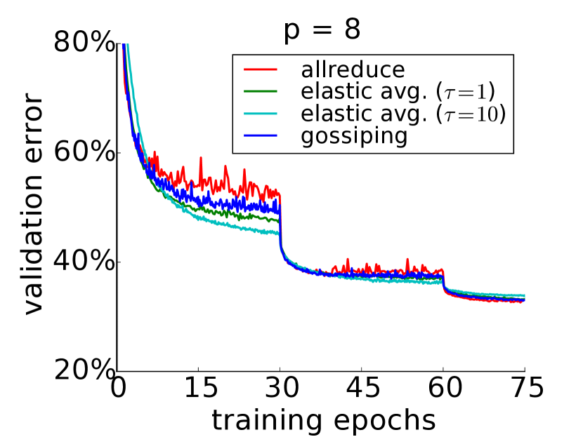
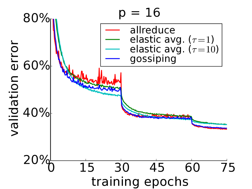
Figure 1: Center-crop validation loss and top-1 error on ImageNet over training wall-clock time and epochs. Shown are: (left) $p=8$ nodes with per-node minibatch size $b=32$, and (right) $p=16$ nodes with per-node minibatch size $b=16$,

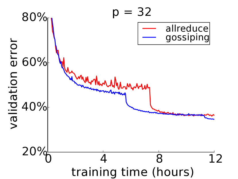
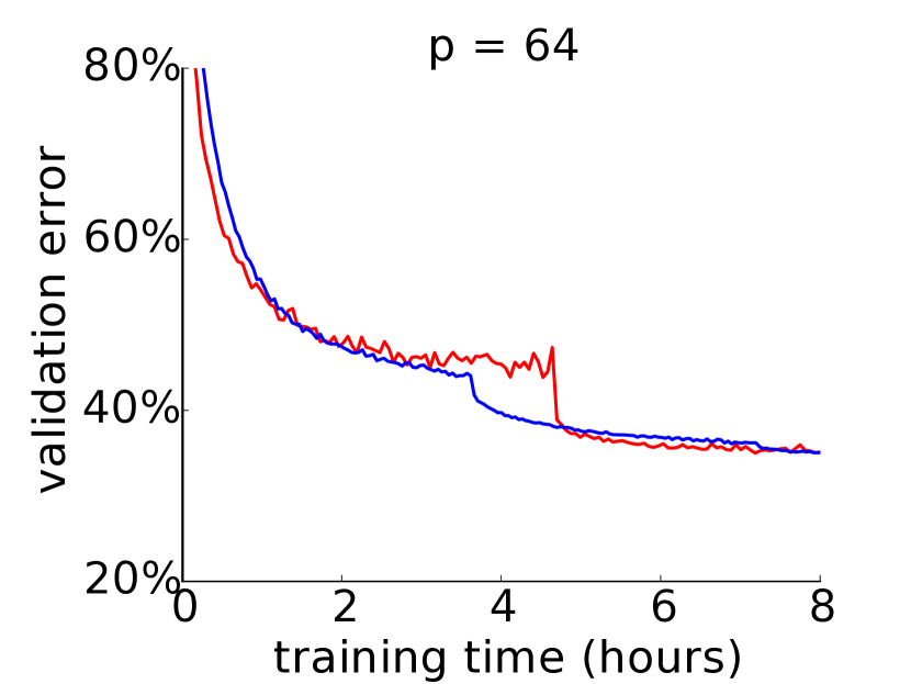
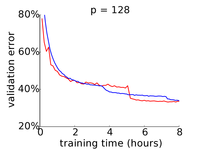
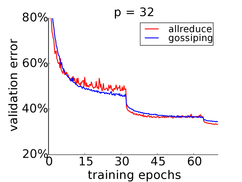
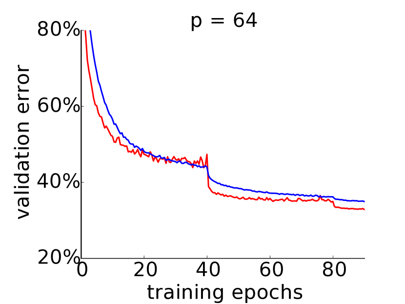
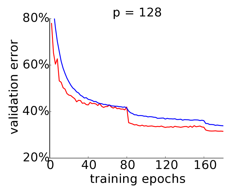
Figure 2: Center-crop validation loss and top-1 error on ImageNet over training wall-clock time and epochs, with different numbers of nodes $p$ and per-node minibatch size $b=16$. Shown are: (left) $p=32$ nodes, (middle) $p=64$ nodes, and (right) $p=128$ nodes.

4.1 Implementation

We implement the communication systems of gossiping SGD and other algorithms using Message Passing Interface (MPI) [19]. Because we wanted to run our code in cluster computing environments with Infiniband or more specialized interconnects, then targeting MPI was the easiest solution. We targeted our code to run on GPUs, using the Nvidia CUDA 7.0 driver and using the cuBLAS and cuDNNv4 [20] libraries for the core computational kernels.

For our experiments up to $p=16$ nodes, we use a local cluster of 16 machines, each one consisting of an Nvidia Kepler K80 dual GPU, an 8-core Intel Haswell E5-1680v2 CPU, and a Mellanox ConnectX-3 FDR $4\times$ Infiniband (56 Gb/s) NIC. We utilize only one GPU per K80.

For our larger scale experiments up to $p=128$ nodes, we used a GPU supercomputer with over 10,000 total nodes. Nodes consist of an Nvidia Kepler K20X GPU and an 8-core AMD Bulldozer Opteron 6274 CPU, and are connected by a Cray Gemini interconnect in a 3D torus configuration.

4.2 Methodology

We chose ResNets [7] for our neural network architecture; specifically, we trained ResNet-18, which is small enough to train rapidly for experimentation, but also possesses features relevant to modern networks, including depth, residual layers, and batch normalization [21]. We ran on the image classification problem of ImageNet consisting of 1.28 million training images and 50,000 validation images divided into 1000 classes [8]. Our data augmentation is as follows: we performed multi-scale training by scaling the shortest dimension of images to between $256$ and $480$ pixels [22], we took random $224\times 224$ crops and horizontal flips, and we added pixelwise color noise [23]. We evaluate validation loss and top-1 error on center crops of the validation set images with the shortest dimension scaled to $256$ pixels.

Unless otherwise noted, we initialized the learning rate to $\alpha=0.1$, then we annealed it twice by a factor of $0.1$. For our experiments with aggregate minibatch size $m=pb=256$, we annealed at exactly 150k and 300k iterations into training. For our experiments with larger aggregate minibatch sizes, we decreased the number of iterations at which the step size was annealed. We used Nesterov momentum of $\mu=0.9$ and weight decay of $\lambda=10^{-4}$. For elastic averaging, we set $\beta=0.8/p$. For all-reduce and gossiping, we used a communication interval of $\tau=1$, i.e. communication occurred every iteration. For gossiping, we used both $\tau=1$ and $\tau=10$ (the latter is recommended in [9]).

4.3 Results

Our first set of experiments compare all-reduce, elastic averaging, and push-gossiping at $p=8$ and $p=16$ with an aggregate minibatch size $m=pb=256$. The results are in Figure 1.

For $p=8$, elastic averaging with a communication delay $\tau=10$ performs ahead of the other methods, Interestingly, all-reduce has practically no synchronization overhead on the system at $p=8$ and is as fast as gossiping. All methods converge to roughly the same minimum loss value.

For $p=16$, gossiping converges faster than elastic averaging with $\tau=10$, and both come ahead of all-reduce. Additionally, elastic averaging with both $\tau=1$ and $\tau=10$ has trouble converging to the same validation loss as the other methods once the step size has been annealed to a small value ($\alpha=0.001$ in this case).

We also perform larger scale experiments at $p=32$ nodes, $p=64$ nodes, and $p=128$ nodes in the GPGPU supercomputing environment. In this environment, elastic averaging did not perform well so we do not show those results here; pull-gossiping also performed better than push-gossiping, so we only show results for pull-gossiping. The results are in Figure 2. At this scale, we begin to see the scaling advantage of synchronous all-reduce SGD. One iteration of gossiping SGD is still faster than one iteration of all-reduce SGD, and gossiping works quickly at the initial step size. But gossiping SGD begins to converge much slower after the step size has annealed.

We note that the training time of SGD can be thought of as the product $(\text{wall-clock time per iteration})\times(\text{number of iterations})$. One observation we made consistent with [4] was the following: letting synchronous all-reduce SGD run for many epochs, it will typically converge to a lower optimal validation loss (or higher validation accuracy) than either elastic averaging or gossiping SGD. We found that letting all-reduce SGD run for over 1 million iterations with a minibatch size of 256 led to a peak top-1 validation accuracy of $68.7\%$. However, elastic averaging often had trouble breaking $67\%$, as did gossiping when the number of nodes was greater than $p=32$. In other words, at larger scales the asynchronous methods require more iterations to convergence despite lower wall-clock time per iteration.

5 Discussion

Revisiting the questions we asked in the beginning:

1. How fast do asynchronous and synchronous SGD algorithms converge at both the beginning of training (large step sizes) and at the end of training (large step sizes)?

   Up to around 32 nodes, asynchronous SGD can converge faster than all-reduce SGD when the step size is large. When the step size is small (roughly $0.001$ or less), gossiping can converge faster than elastic averaging, but all-reduce SGD converges most consistently.

2. How does the convergence behavior of asynchronous and synchronous distributed SGD vary with the number of nodes?

   Both elastic averaging and gossiping seem to converge faster than synchronous all-reduce SGD with fewer nodes (up to 16–32 nodes). With more nodes (up to a scale of 100 nodes), all-reduce SGD can consistently converge to a high-accuracy solution, whereas asynchronous methods seem to plateau at lower accuracy. In particular, the fact that gossiping SGD does not scale as well as does synchronous SGD with more nodes suggests that the asynchrony and the pattern of communication, rather than the amount of communication (both methods have low amounts of communication), are responsible for the difference in convergence.

In this work, we focused on comparing the scaling of synchronous and asynchronous SGD methods on a supervised learning problem on two platforms: a local GPU cluster and a GPU supercomputer. However, there are other platforms that are relevant for researchers, depending on what resources they have available. These other platforms include multicore CPUs, multi-GPU single servers, local CPU clusters, and cloud CPU/GPU instances, and we would expect to observe somewhat different results compared to the platforms tested in this work.

While our experiments were all in the setting of supervised learning (ImageNet image classification), the comparison between synchronous and asynchronous parallelization of learning may differ in other settings; c.f. recent results on asynchronous methods in deep reinforcement learning [24]. Additionally, we specifically used convolutional neural networks in our supervised learning experiments, which because of their high arithmetic intensity (high ratio of floating point operations to memory footprint) have a different profile from networks with many fully connected operations, including most recurrent networks.

Finally, we exclusively looked at SGD with Nesterov momentum as the underlying algorithm to be parallelized/distributed. Adaptive versions of SGD such as RMSProp [25] and Adam [26] are also widely used in deep learning, and their corresponding distributed versions may have additional considerations (e.g. sharing the squared gradients in [24]).

References

6 Appendix

6.1 Analysis

The analysis below loosely follow the arguments presented in, and use a combination of techniques appearing from [17,16,10,18,9].

For ease of exposition and notation, we focus our attention on the case of univariate strongly convex function $f$ with Lipschitz gradients. (Since the sum of squares errors are additive in vector components, the arguments below generalize to the case of multivariate functions.) We assume that the gradients of the function $f$ can be sampled by all processors independently up to additive noise with zero mean and bounded variance. (Gaussian noise satisfy these assumptions, for example.) We also assume a fully connected network where all processors are able to communicate with all other processors. Additional assumptions are introduced below as needed.

We denote by $\theta_{t}=\begin{bmatrix}\theta_{t,1},\cdots,\theta_{t,p}\end{bmatrix}^{T}$ the vector containing all local parameter values at time step $t$, we denote by $\theta_{\ast}$ the optimal value of the objective function $f$, and we denote by $\bar{\theta}_{t}\equiv\tfrac{1}{p}\sum_{i=1}^{p}\theta_{t,i}$ the spatial average of the local parameters taken at time step $t$.

We derive bounds for the following two quantities:

• $\mathbb{E}[\|\theta_{t}-\theta_{\ast}\mathbf{1}\|^{2}]$, the squared sum of the local parameters’ deviation from the optimum $\theta_{\ast}$
  

• $\mathbb{E}[\|\theta_{t}-\bar{\theta}_{t}\mathbf{1}\|^{2}]$, the squared sum of the local parameters’ deviation from the mean $\bar{\theta}_{t}=\frac{1}{p}\sum_{i=1}^{p}\theta_{t,i}$

where the expectation is taken with respect to both the “pull” parameter choice and the gradient noise term. In the literature [18], the latter is usually referred to as “agent agreement” or “agent consensus”.

6.1.1 Synchronous pull-gossip algorithm

We begin by analyzing the synchronous version of the pull-gossip algorithm described in Algorithm 3. For each processor $i$, let $j_{i}$ denote the processor, chosen uniformly randomly from $\{1,\cdots,p\}$ from which processor $i$ “pulls” parameter values. The update for each $\theta_{t,i}$ is given by

$$\theta_{t+1,i}=\frac{1}{2}\left(\theta_{t,i}+\theta_{t,j_{i}}\right)-\alpha_{t}\left(\nabla f\left(\frac{1}{2}\left(\theta_{t,i}+\theta_{t,j_{i}}\right);X_{t,i}\right)+\xi_{t,i}\right)$$ (12)

We prove the following rate of convergence for the synchronous pull-gossip algorithm.

Theorem 2.

Let $f$ be a $m$-strongly convex function with $L$-Lipschitz gradients. Assume that we can sample gradients $g=\nabla f(\theta;X_{i})+\xi_{i}$ with additive noise with zero mean $\mathbb{E}[\xi_{i}]=0$ and bounded variance $\mathbb{E}[\xi_{i}^{T}\xi_{i}]\leq\sigma^{2}$. Then, running the synchronous pull-gossip algorithm as outlined above with step size $0<\alpha\leq\tfrac{2}{m+L}$, the expected sum of squares convergence of the local parameters to the optimal $\theta_{\ast}$ is bounded by

$$\mathbb{E}[\|\theta_{t}-\theta_{\ast}\mathbf{1}\|^{2}] \leq\left(1-2\alpha\frac{mL}{m+L}\right)^{t}\|\theta_{0}-\theta_{\ast}\mathbf{1}\|^{2}+p\alpha\sigma^{2}\frac{m+L}{2mL}$$ (13)

Remark.

Note that this bound is characteristic of SGD bounds, where the iterates converge to within some ball around the optimal solution. It can be shown by induction that a decreasing step size schedule of $\alpha_{t}\sim\mathcal{O}(1/pt)$ can be used to achieve a convergence rate of $\mathcal{O}(1/t)$.

Proof.

For notational simplicity, we denote $\theta_{t,i,j_{i}}\equiv\frac{1}{2}\left(\theta_{t,i}+\theta_{t,j_{i}}\right)$, and drop the $X_{t,i}$ in the gradient term. We tackle the first quantity by conditioning on the previous parameter values and expanding as

$$\mathbb{E}[\|\theta_{t+1}-\theta_{\ast}\mathbf{1}\|^{2}\,|\,\theta_{t}] =\mathbb{E}\left[\sum_{i=1}^{p}\left(\theta_{t,i,j_{i}}-\theta_{\ast}\right)^{T}\left(\theta_{t,i,j_{i}}-\theta_{\ast}\right)\,\Big{|}\,\theta_{t}\right]$$ (14)

$$-2\alpha_{t}\mathbb{E}\left[\sum_{i=1}^{p}\nabla f(\theta_{t,i,j_{i}})^{T}(\theta_{t,i,j_{i}}-\theta_{\ast})\,\Big{|}\,\theta_{t}\right]$$ (15)

$$-2\alpha_{t}\mathbb{E}\left[\sum_{i=1}^{p}\xi_{t,i}^{T}\left(\theta_{t,i,j_{i}}-\theta_{\ast}\right)\,\Big{|}\,\theta_{t}\right]$$ (16)

$$+\alpha_{t}^{2}\left[\sum_{i=1}^{p}\left(\nabla f(\theta_{t,i,j_{i}})+\xi_{t,i}\right)^{T}\left(\nabla f(\theta_{t,i,j_{i}})+\xi_{t,i}\right)\,\Big{|}\,\theta_{t}\right]$$ (17)

Recalling that strongly convex functions satisfy [17], $\forall x,z$,

$$(\nabla f(x)-\nabla f(z))^{T}(x-z)$$ (18)

$$\geq\frac{mL}{m+L}(x-z)^{T}(x-z)+\frac{1}{m+L}(\nabla f(x)-\nabla f(z))^{T}(\nabla f(x)-\nabla f(z))$$

we can use this inequality, with $x=\theta_{t,i,j_{i}}$ and $z=\theta_{\ast}$ to bound the term in (15):

$$-2\alpha_{t}\mathbb{E}\left[\sum_{i=1}^{p}\nabla f(\theta_{t,i,j_{i}})^{T}(\theta_{t,i,j_{i}}-\theta_{\ast})\,\Big{|}\,\theta_{t}\right]$$ (19)

$$\leq-\frac{2\alpha_{t}mL}{m+L}\mathbb{E}\left[\sum_{i=1}^{p}(\theta_{t,i,j_{i}}-\theta_{\ast})^{T}(\theta_{t,i,j_{i}}-\theta_{\ast})\,\Big{|}\,\theta_{t}\right]-\frac{2\alpha_{t}}{m+L}\mathbb{E}\left[\sum_{i=1}^{p}\nabla f(\theta_{t,i,j_{i}})^{T}\nabla f(\theta_{t,i,j_{i}})\,\Big{|}\,\theta_{t}\right]$$

Using (6.1.1), and regrouping terms in (14)-(17), we obtain

$$\mathbb{E}[\|\theta_{t+1}-\theta_{\ast}\mathbf{1}\|^{2}\,|\,\theta_{t}] \leq\left(1-2\alpha_{t}\frac{mL}{m+L}\right)\mathbb{E}\left[\sum_{i=1}^{p}\left(\theta_{t,i,j_{i}}-\theta_{\ast}\right)^{T}\left(\theta_{t,i,j_{i}}-\theta_{\ast}\right)\,\Big{|}\,\theta_{t}\right]$$ (20)

$$+\left(\alpha_{t}^{2}-2\alpha_{t}\frac{1}{m+L}\right)\mathbb{E}\left[\sum_{i=1}^{p}\nabla f(\theta_{t,i,j_{i}})^{T}\nabla f(\theta_{t,i,j_{i}})\,\Big{|}\,\theta_{t}\right]$$ (21)

$$+\alpha^{2}_{t}\mathbb{E}\left[\sum_{i=1}^{p}\xi_{t,i}^{T}\xi_{t,i}\,\Big{|}\,\theta_{t}\right]$$ (22)

In the above expression, we have dropped the terms linear in $\xi_{t,i}$, using the assumption that these noise terms vanish in expectation. In addition, if the step size parameter $\alpha$ is chosen sufficiently small, $0<\alpha_{t}\leq\frac{2}{m+L}$, then the second term in (21) can also be dropped. The expression we must contend with is

$$\mathbb{E}[\|\theta_{t+1}-\theta_{\ast}\mathbf{1}\|^{2}\,|\,\theta_{t}] \leq\left(1-2\alpha_{t}\frac{mL}{m+L}\right)\mathbb{E}\left[\sum_{i=1}^{p}\left(\theta_{t,i,j_{i}}-\theta_{\ast}\right)^{T}\left(\theta_{t,i,j_{i}}-\theta_{\ast}\right)\,\Big{|}\,\theta_{t}\right]+\alpha^{2}_{t}p\sigma^{2}$$ (23)

Using the definition of $\theta_{t,i,j_{i}}$, we can verify that the following matrix relation holds.

$$\begin{bmatrix}\theta_{t,1,j_{1}}-\theta_{\ast}\\ \vdots\\ \theta_{t,i,j_{i}}-\theta_{\ast}\\ \vdots\\ \theta_{t,p,j_{p}}-\theta_{\ast}\end{bmatrix} =\begin{bmatrix}\tfrac{1}{2}&&&\tfrac{1}{2}&\\ &\ddots&&&\\ &\tfrac{1}{2}&\tfrac{1}{2}&&&\\ &&&\ddots&\\ \tfrac{1}{2}&&&&\tfrac{1}{2}\end{bmatrix}\begin{bmatrix}\theta_{t,1}-\theta_{\ast}\\ \vdots\\ \theta_{t,i}-\theta_{\ast}\\ \vdots\\ \theta_{t,p}-\theta_{\ast}\end{bmatrix}\equiv M_{I}(\theta_{t}-\theta_{\ast}\mathbf{1})$$ (24)

where the random matrix $M_{I}$ depends on the random index set $I=\{j_{i}\}_{i=1}^{p}$ of uniformly randomly drawn indices. $M_{I}$ has two entries in each row, one on the diagonal, and one appearing in the $j_{i}$th column, and is a right stochastic matrix but need not be doubly stochastic.

We can express this matrix as

$$M_{I} =\frac{1}{2}\sum_{i=1}^{p}e_{i}(e_{i}+e_{j_{i}})^{T}$$

and compute its second moment

$$\mathbb{E}[M_{I}^{T}M_{I}] =\frac{1}{4}\,\mathbb{E}\left[\left(I+\sum_{i=1}^{p}e_{i}e_{j_{i}}^{T}\right)^{T}\left(I+\sum_{i=1}^{p}e_{i}e_{j_{i}}^{T}\right)\right]$$ (25)

$$=\frac{1}{2}\left(I+\frac{1}{p}\mathbf{1}\mathbf{1}^{T}\right)$$ (26)

$$=Q\begin{bmatrix}1&&&\\ &\tfrac{1}{2}&&\\ &&\ddots&\\ &&&\tfrac{1}{2}\end{bmatrix}Q^{T}$$ (27)

where in the last line, the orthogonal diagonalization reveals that the eigenvalues of this matrix are bounded by $\frac{1}{2}\leq\lambda_{i}\leq 1$.

Using (27), we can further simply (23) to

$$\mathbb{E}[\|\theta_{t+1}-\theta_{\ast}\mathbf{1}\|^{2}\,|\,\theta_{t}] \leq\left(1-2\alpha_{t}\frac{mL}{m+L}\right)(\theta_{t}-\theta_{\ast}\mathbf{1})^{T}\mathbb{E}\left[M_{I}^{T}M_{I}\right](\theta_{t}-\theta_{\ast}\mathbf{1})+\alpha^{2}_{t}p\sigma^{2}$$ (28)

$$\leq\left(1-2\alpha_{t}\frac{mL}{m+L}\right)\|\theta_{t}-\theta_{\ast}\mathbf{1}\|^{2}+\alpha^{2}_{t}p\sigma^{2}$$ (29)

Assuming a constant step size $\alpha_{t}\equiv\alpha$, the above recursion can be unrolled to derive the bound

$$\mathbb{E}[\|\theta_{t}-\theta_{\ast}\mathbf{1}\|^{2}] \leq\left(1-2\alpha\frac{mL}{m+L}\right)^{t}\|\theta_{0}-\theta_{\ast}\mathbf{1}\|^{2}+p\alpha\sigma^{2}\frac{m+L}{2mL}$$ (30)

We note that the above bound is characteristic of SGD bounds, where the iterates converge to a ball around the optimal solution, whose radius now depends on the number of processors $p$, in addition to the step size $\alpha$ and the variance of the gradient noise $\sigma^{2}$.

∎

6.1.2 Asynchronous pull-gossip algorithm

We provide similar analysis for the asynchronous version of the pull-gossip algorithm. As is frequently done in the literature, we model the time steps as the ticking of local clocks governed by Poisson processes. More precisely, we assume that each processor has a clock which ticks with a rate $1$ Poisson process. A master clock which ticks whenever a local processor clock ticks is then governed by a rate $p$ Poisson process, and a time step in the algorithm is defined as whenever the master clock ticks. Since each master clock tick corresponds to the tick of some local clock on processor $i$, this in turn marks the time step at which processor $i$ “pulls” the parameter values from the uniformly randomly chosen processor $j_{i}$. Modeling the time steps by Poisson processes provide nice theoretical properties, i.e. the inter-tick time intervals are i.i.d. exponential variables of rate $p$, and the local clock $i$ which causes each master clock tick is i.i.d. drawn from $\{1,\cdots,p\}$, to name a few. For an in depth analysis of this model, and results that relate the master clock ticks to absolute time, please see [16].

The main variant implemented is the pull-gossip with fresh parameters in subsection 6.2.2. The update at each time step is given by

$$\left\{\begin{array}[]{ll}\theta_{t+1,i}=(1-\beta)\left(\theta_{t,i}-\alpha_{t}\left(\nabla f(\theta_{t,i})+\xi_{t,i}\right)\right)+\beta\theta_{t,j_{i}}&\\ \theta_{t+1,k}=\theta_{t,k}&\,\text{ , for }\,k\neq i\end{array}\right.$$

$$\text{where }\xi_{t,i}\text{ is the gradient noise }$$

Note in the implementation we use $\beta=1/2$, however in the analysis we retain the $\beta$ parameter for generality.

We have the following convergence result.

Theorem 3.

Let $f$ be a $m$-strongly convex function with $L$-Lipschitz gradients. Assume that we can sample gradients $g=\nabla f(\theta;X_{i})+\xi_{i}$ with additive noise with zero mean $\mathbb{E}[\xi_{i}]=0$ and bounded variance $\mathbb{E}[\xi_{i}^{T}\xi_{i}]\leq\sigma^{2}$. Then, running the asynchronous pull-gossip algorithm with the time model as described, with constant step size $0<\alpha\leq\tfrac{2}{m+L}$, the expected sum of squares convergence of the local parameters to the optimal $\theta_{\ast}$ is bounded by

$$\mathbb{E}[\|\theta_{t}-\theta_{\ast}\mathbf{1}\|^{2}]\leq\left(1-\frac{2\alpha}{p}\frac{mL}{m+L}\right)^{t}\|\theta_{0}-\theta_{\ast}\mathbf{1}\|^{2}+p\alpha\sigma^{2}\frac{m+L}{2mL}$$ (31)

Furthermore, with the additional assumption that the gradients are uniformly bounded as $\sup|\nabla f(\theta)|\leq C$, the expected sum of squares convergence of the local parameters to the mean $\bar{\theta}_{t}$ is bounded by

$$\mathbb{E}[\|\theta_{t}-\bar{\theta}_{t}\mathbf{1}\|^{2}] \leq\left(\lambda\left(1-\frac{\alpha\,m}{p}\right)\right)^{t}\|\theta_{0}-\bar{\theta}_{0}\mathbf{1}\|^{2}+\frac{\lambda\alpha^{2}(C^{2}+\sigma^{2})}{1-\lambda\left(1-\frac{\alpha\,m}{p}\right)}$$ (32)

$$\text{ where }\lambda =1-\frac{2\beta(1-\beta)}{p}-\frac{2\beta^{2}}{p}$$ (33)

Remark.

Note again that this bound is characteristic of SGD bounds, with the additional dependence on $p$, the number of processors.

Proof.

For simplicity of notation, we denote $g_{t,i}\equiv\nabla f(\theta_{t,i})+\xi_{t,i}$. We can write the asynchronous iteration step in matrix form as

$$\begin{bmatrix}\theta_{t+1,1}-\theta_{\ast}\\ \vdots\\ \theta_{t+1,i}-\theta_{\ast}\\ \vdots\\ \theta_{t+1,j_{i}}-\theta_{\ast}\\ \vdots\\ \theta_{t+1,p}-\theta_{\ast}\end{bmatrix} =\begin{bmatrix}1&&&&&&\\ &\ddots&&&&&\\ &&1-\beta&&\beta&&\\ &&&\ddots&&&\\ &&&&1&&\\ &&&&&\ddots&\\ &&&&&&1\end{bmatrix}\left(\begin{bmatrix}\theta_{t,1}-\theta_{\ast}\\ \vdots\\ \theta_{t,i}-\theta_{\ast}\\ \vdots\\ \theta_{t,j_{i}}-\theta_{\ast}\\ \vdots\\ \theta_{t,p}-\theta_{\ast}\end{bmatrix}-\alpha_{t}\begin{bmatrix}0\\ \vdots\\ g_{t,i}\\ \vdots\\ 0\\ \vdots\\ 0\end{bmatrix}\right)$$ (34)

$$\equiv D_{i,j_{i}}\left((\theta_{t}-\theta_{\ast})-\alpha_{t}g_{t}\right)$$ (35)

The random matrix $D_{i,j_{i}}$ depends on the indices $i$ and $j_{i}$, both of which are uniformly randomly drawn from $\{1,\cdots,p\}$. For notational convenience we will drop the subscripts, but we keep in mind that the expectation below is taken with respect to the randomly chosen indices. We can express the matrix as

$$D =I+\beta e_{i}(ej_{i}-e_{i})^{T}$$ (36)

and compute its second moment as

$$\mathbb{E}[D^{T}D] =\left(1-\frac{2\beta(1-\beta)}{p}\right)\mathbf{I}+\frac{2\beta(1-\beta)}{p^{2}}\mathbf{1}\mathbf{1}^{T}$$ (37)

$$=Q\begin{bmatrix}1&&&\\ &1-\frac{2\beta(1-\beta)}{p}&&\\ &&\ddots&\\ &&&1-\frac{2\beta(1-\beta)}{p}\end{bmatrix}Q^{T}$$ (38)

The orthogonal diagonalization reveals that the eigenvalues of this matrix are bounded by $1-\tfrac{2\beta(1-\beta)}{p}\leq\lambda_{i}\leq 1$.

Using (38), we can expand and bound the expected sum of squares deviation by

$$\mathbb{E}[\|\theta_{t+1}-\theta_{\ast}\mathbf{1}\|^{2}|\theta_{t}]$$

$$=\mathbb{E}\left[((\theta_{t}-\theta_{\ast}\mathbf{1})-\alpha_{t}g_{t})^{T}D^{T}D((\theta_{t}-\theta_{\ast}\mathbf{1})-\alpha_{t}g_{t})\right]$$ (39)

$$\leq\mathbb{E}\left[\|(\theta_{t}-\theta_{\ast}\mathbf{1})-\alpha_{t}g_{t}\|^{2}\right]$$ (40)

$$=\|\theta_{t}-\theta_{\ast}\mathbf{1}\|^{2}-\frac{2\alpha_{t}}{p}\sum_{i=1}^{p}\nabla f(\theta_{t,i})^{T}(\theta_{t,i}-\theta_{\ast})+\frac{\alpha_{t}^{2}}{p}\sum_{i=1}^{p}\nabla f(\theta_{t,i})^{T}\nabla f(\theta_{t,i})+\frac{\alpha_{t}^{2}}{p}\sum_{i=1}^{p}\xi_{t,i}^{T}\xi_{t,i}$$ (41)

where in the last line, we have dropped terms that are linear in $\xi_{t,i}$ by using the zero mean assumption. Making use of the strong convexity inequality (6.1.1), we can bound the second term in the above sum by

$$-\nabla f(\theta_{t,i})^{T}(\theta_{t,i}-\theta_{\ast})\leq-\frac{mL}{m+L}(\theta_{t,i}-\theta_{\ast})^{T}(\theta_{t,i}-\theta_{\ast})-\frac{1}{m+L}\nabla f(\theta_{t,i})^{T}\nabla f(\theta_{t,i})$$

and rearrange the terms in (41) to derive

$$\mathbb{E}[\|\theta_{t+1}-\theta_{\ast}\mathbf{1}\|^{2}|\theta_{t}] \leq\left(1-\frac{2\alpha_{t}}{p}\frac{mL}{m+L}\right)\|\theta_{t}-\theta_{\ast}\mathbf{1}\|^{2}$$ (42)

$$+\left(\frac{\alpha_{t}^{2}}{p}-\frac{2\alpha_{t}}{p}\frac{1}{m+L}\right)\sum_{i=1}^{p}\nabla f(\theta_{t,i})^{T}\nabla f(\theta_{t,i})$$ (43)

$$+\alpha_{t}^{2}\sigma^{2}$$ (44)

The term in (43) can be dropped if $\alpha_{t}$ is chosen sufficiently small, with the now familiar requirement that $0<\alpha_{t}<\frac{2}{m+L}$. Assuming this is the case, we have

$$\mathbb{E}[\|\theta_{t+1}-\theta_{\ast}\mathbf{1}\|^{2}|\theta_{t}] \leq\left(1-\frac{2\alpha_{t}}{p}\frac{mL}{m+L}\right)\|\theta_{t}-\theta_{\ast}\mathbf{1}\|^{2}+\alpha_{t}^{2}\sigma^{2}$$ (45)

Assuming a constant step size $\alpha_{t}\equiv\alpha$, we can use the law of iterated expectations to unroll the recursion, giving

$$\mathbb{E}[\|\theta_{t}-\theta_{\ast}\mathbf{1}\|^{2}]\leq\left(1-\frac{2\alpha}{p}\frac{mL}{m+L}\right)^{t}\|\theta_{0}-\theta_{\ast}\mathbf{1}\|^{2}+p\alpha\sigma^{2}\frac{m+L}{2mL}$$ (46)

Note this is the same convergence rate guarantee as stochastic gradient descent with an extra factor of $p$, albeit the coordination amongst processors required to adjust the step size is unrealistic in practice.

Next, we prove the bound on the processors’ local parameters’ convergence to each other / to the mean, $\mathbb{E}[\|\theta_{t}-\bar{\theta}_{t}\mathbf{1}\|^{2}]$.

First, we write the spatial parameter average in vector form as

$$\bar{\theta}_{t}=\frac{1}{p}\mathbf{1}^{T}\theta_{t}$$ (47)

With $D$ as previously defined in (35), we can write

$$\bar{\theta}_{t+1}\mathbf{1} =\frac{1}{p}\mathbf{1}^{T}\theta_{t+1}\mathbf{1}=\frac{1}{p}\mathbf{1}^{T}D(\theta_{t}-\alpha g_{t})\mathbf{1}$$ (48)

and so the term we wish to bound can be expanded as

$$\|\theta_{t+1}-\bar{\theta}_{t+1}\mathbf{1}\|^{2} =(\theta_{t}-\alpha_{t}g_{t})^{T}\left(D^{T}D-\frac{1}{p}D^{T}\mathbf{1}\mathbf{1}^{T}D\right)(\theta_{t}-\alpha_{t}g_{t})$$ (49)

In addition to the diagonalization we previous calculated in (38) (reproduced below for convenience), we calculate some other useful diagonalizations.

$$\mathbb{E}[D^{T}D] =\left(1-\frac{2\beta(1-\beta)}{p}\right)\mathbf{I}+\frac{2\beta(1-\beta)}{p^{2}}\mathbf{1}\mathbf{1}^{T}$$ (50)

$$=Q\begin{bmatrix}1&&&\\ &1-\frac{2\beta(1-\beta)}{p}&&\\ &&\ddots&\\ &&&1-\frac{2\beta(1-\beta)}{p}\end{bmatrix}Q^{T}$$ (51)

$$\mathbb{E}[D^{T}\mathbf{1}\mathbf{1}^{T}D] =\frac{2\beta^{2}}{p}\mathbf{I}+\left(1-\frac{2\beta^{2}}{p^{2}}\right)\mathbf{1}\mathbf{1}^{T}$$ (52)

$$=Q\begin{bmatrix}p&&&\\ &\frac{2\beta^{2}}{p}&&\\ &&\ddots&\\ &&&\frac{2\beta^{2}}{p}\end{bmatrix}Q^{T}$$ (53)

$$\mathbb{E}\left[D^{T}D-\frac{1}{p}D^{T}\mathbf{1}\mathbf{1}^{T}D\right] =\left(1-\frac{2\beta(1-\beta)}{p}-\frac{2\beta^{2}}{p^{2}}\right)\mathbf{I}+\left(\frac{2\beta(1-\beta)}{p^{2}}-\frac{1}{p}\left(1-\frac{2\beta^{2}}{p^{2}}\right)\right)\mathbf{1}\mathbf{1}^{T}$$ (54)

$$=Q\begin{bmatrix}0&&&\\ &1-\frac{2\beta(1-\beta)}{p}-\frac{2\beta^{2}}{p^{2}}&&\\ &&\ddots&\\ &&&1-\frac{2\beta(1-\beta)}{p}-\frac{2\beta^{2}}{p^{2}}\end{bmatrix}Q^{T}$$ (55)

We note that all three matrices are diagonalized by the same orthogonal matrix $Q$. Furthermore, the first eigenvector, corresponding to the eigenvalues $1$, $p$, $0$ respectively, is $q_{1}=\frac{1}{\sqrt{p}}\mathbf{1}$.

Continuing from (49), we take the expectation and use (55) to further bound the expression. In the computation below we use $\lambda\equiv 1-\frac{2\beta(1-\beta)}{p}-\frac{2\beta^{2}}{p}$ as a notational shorthand.

$$\mathbb{E}[\|\theta_{t+1}-\bar{\theta}_{t+1}\mathbf{1}\|^{2}|\theta_{t}]$$

$$=\mathbb{E}\left[(\theta_{t}-\alpha_{t}g_{t})^{T}\left(D^{T}D-\frac{1}{p}D^{T}\mathbf{1}\mathbf{1}^{T}D\right)(\theta_{t}-\alpha_{t}g_{t})\right]$$ (56)

$$\leq\mathbb{E}\left[\lambda\|(\theta_{t}-\bar{\theta}_{t}\mathbf{1})-\alpha_{t}g_{t}\|^{2}\right]$$ (57)

$$=\lambda\left(\|\theta_{t}-\bar{\theta}_{t}\mathbf{1}\|^{2}-\frac{2\alpha_{t}}{p}\sum_{i=1}^{p}\nabla f(\theta_{t,i})^{T}(\theta_{t,i}-\bar{\theta}_{t})+\frac{\alpha_{t}^{2}}{p}\sum_{i=1}^{p}\nabla f(\theta_{t,i})^{T}\nabla f(\theta_{t,i})+\frac{\alpha_{t}^{2}}{p}\sum_{i=1}^{p}\xi_{t,i}^{T}\xi_{t,i}\right)$$ (58)

$$\leq\lambda\left(\|\theta_{t}-\bar{\theta}_{t}\mathbf{1}\|^{2}+\frac{2\alpha_{t}}{p}\sum_{i=1}^{p}\left(f(\bar{\theta}_{t})-f(\theta_{t,i})\right)-\frac{\alpha_{t}m}{p}\sum_{i=1}^{p}(\theta_{i,t}-\bar{\theta}_{t})^{2}+\frac{\alpha_{t}^{2}}{p}\sum_{i=1}^{p}(C^{2}+\sigma^{2})\right)$$ (59)

$$\leq\lambda\left(1-\frac{\alpha_{t}\,m}{p}\right)\|\theta_{t}-\bar{\theta}_{t}\mathbf{1}\|^{2}+\lambda\alpha_{t}^{2}(C^{2}+\sigma^{2})$$ (60)

In (58) and (59), we have used the definition of strong convexity and convexity respectively.

Finally, taking constant step size $\alpha_{t}\equiv\alpha$, and using the law of iterated expectations to unroll the recursion, we have

$$\mathbb{E}[\|\theta_{t}-\bar{\theta}_{t}\mathbf{1}\|^{2}] \leq\left(\lambda\left(1-\frac{\alpha\,m}{p}\right)\right)^{t}\|\theta_{0}-\bar{\theta}_{0}\mathbf{1}\|^{2}+\frac{\lambda\alpha^{2}(C^{2}+\sigma^{2})}{1-\lambda\left(1-\frac{\alpha\,m}{p}\right)}$$ (61)

When the step size $\alpha$ is small and the number of processors $p$ is large, the quantity $\lambda\left(1-\frac{\alpha\,m}{p}\right)=\left(1-\frac{2\beta(1-\beta)}{p}-\frac{2\beta^{2}}{p}\right)\left(1-\frac{\alpha\,m}{p}\right)$ is well approximated by $1-\frac{2\beta(1-\beta)}{p}-\frac{2\beta^{2}}{p}-\frac{\alpha m}{p}$, which makes clear the dependence of the rate on the parameter $p$. ∎

6.2 Gossip variants

6.2.1 Gossip with stale parameters (gradient step and gossip at the same time)

Consider a one-step distributed consensus gradient update:

$$\theta_{i,t+1} =\theta_{i,t}-\alpha\nabla f(\theta_{i,t};X_{i})-\beta\left(\theta_{i,t}-\frac{1}{p}\sum_{j=1}^{p}\theta_{j,t}\right).$$ (62)

If we replace the distributed mean $\frac{1}{p}\sum_{j=1}^{p}\theta_{j,t}$ with an unbiased one-sample estimator $\theta_{j_{i,t},t}$, such that $j_{i,t}\sim\text{Uniform}(\{1,\ldots,p\})$ and $\mathbb{E}[\theta_{j_{i,t},t}]=\frac{1}{p}\sum_{j=1}^{p}\theta_{j,t}$, then we derive the gossiping SGD update:

$$\theta_{i,t+1} =\theta_{i,t}-\alpha\nabla f(\theta_{i,t};X_{i})-\beta(\theta_{i,t}-\theta_{j_{i,t},t})$$ (63)

$$=(1-\beta)\theta_{i,t}+\beta\theta_{j_{i,t},t}-\alpha\nabla f(\theta_{i,t};X_{i}).$$ (64)

6.2.2 Gossip with fresh parameters (gradient step before gossip)

Consider a two-step distributed consensus gradient update:

$$\theta_{i,t}^{\prime} =\theta_{i,t}-\alpha\nabla f(\theta_{i,t};X_{i})$$ (65)

$$\theta_{i,t+1} =\theta_{i,t}^{\prime}-\beta\left(\theta_{i,t}^{\prime}-\frac{1}{p}\sum_{j=1}^{p}\theta_{j,t}^{\prime}\right).$$ (66)

If we replace the distributed mean $\frac{1}{p}\sum_{j=1}^{p}\theta_{j,t}^{\prime}$ with an unbiased one-sample estimator $\theta_{j_{i,t},t}^{\prime}$, such that $j_{i,t}\sim\text{Uniform}(\{1,\ldots,p\})$ and $\mathbb{E}[\theta_{j_{i,t},t}^{\prime}]=\frac{1}{p}\sum_{j=1}^{p}\theta_{j,t}^{\prime}$, then we derive the gossiping SGD update:

$$\theta_{i,t}^{\prime} =\theta_{i,t}-\alpha\nabla f(\theta_{i,t};X_{i})$$ (67)

$$\theta_{i,t+1} =\theta_{i,t}^{\prime}-\beta(\theta_{i,t}^{\prime}-\theta_{j_{i,t},t}^{\prime})$$ (68)

$$=(1-\beta)\theta_{i,t}^{\prime}+\beta\theta_{j_{i,t},t}^{\prime}.$$ (69)

6.3 Implementation details

We provide some more details on our implementation of deep convolutional neural network training in general.

6.3.1 ImageNet data augmentation

We found that multi-scale training could be a significant performance bottleneck due to the computational overhead of resizing images, even when using multiple threads and asynchronous data loading. To remedy this, we used fast CUDA implementations of linear and cubic interpolation filters to perform image scaling during training on the GPU. We also preprocessed ImageNet images such that their largest dimension was no larger than the maximum scale (in our case, 480 pixels).

6.3.2 ResNet implementation

We implemented ResNet-18 using stacked residual convolutional layers with $1\times 1$ projection shortcuts. We used the convolution and batch normalization kernels from cuDNNv4. The highest ImageNet validation set accuracy (center crop, top-1) our implementation of ResNets achieved was about 68.7% with the aforementioned multi-scale data augmentation; we note that researchers at Facebook independently reproduced ResNet with a more sophisticated data augmentation scheme and achieved 69.6% accuracy using the same evaluation methodology on their version of ResNet-18.

References

• Wu et al. [2015] Ren Wu, Shengen Yan, Yi Shan, Qingqing Dang, and Gang Sun. Deep Image: Scaling up Image Recognition. arXiv preprint arXiv:1501.02876, 2015.
• Iandola et al. [2015] Forrest N. Iandola, Khalid Ashraf, Matthew W. Moskewicz, and Kurt Keutzer. FireCaffe: near-linear acceleration of deep neural network training on compute clusters. arXiv preprint arXiv:1511.00175, 2015.
• Das et al. [2016] Dipankar Das, Sasikanth Avancha, Dheevatsa Mudigere, Karthikeyan Vaidynathan, Srinivas Sridharan, Dhiraj Kalamkar, Bharat Kaul, and Pradeep Dubey. Distributed Deep Learning Using Synchronous Stochastic Gradient Descent. arXiv preprint arXiv:1602.06709, 2016.
• Chen et al. [2016] Jianmin Chen, Rajat Monga, Samy Bengio, and Rafal Jozefowicz. Revisiting Distributed Synchronous SGD. arXiv preprint arXiv:1604.00981, 2016.
• Dean et al. [2012] Jeffrey Dean, Greg Corrado, Rajat Monga, Kai Chen, Matthieu Devin, Mark Mao, Andrew Senior, Paul Tucker, Ke Yang, Quoc V. Le, and Andrew Y. Ng. Large Scale Distributed Deep Networks. In Advances in Neural Information Processing Systems 25, pages 1223–1231, 2012.
• Chilimbi et al. [2014] Trishul Chilimbi, Yutaka Suzue, Johnson Apacible, and Karthik Kalyanaraman. Project Adam: Building an Efficient and Scalable Deep Learning Training System. In 11th USENIX Symposium on Operating Systems Design and Implementation, pages 571–582, 2014.
• He et al. [2015] Kaiming He, Xiangyu Zhang, Shaoqing Ren, and Jian Sun. Deep Residual Learning for Image Recognition. arXiv preprint arXiv:1512.03385, 2015.
• Russakovsky et al. [2015] Olga Russakovsky, Jia Deng, Hao Su, Jonathan Krause, Sanjeev Satheesh, Sean Ma, Zhiheng Huang, Andrej Karpathy, Aditya Khosla, Michael Bernstein, Alexander C. Berg, and Fei-Fei Li. ImageNet Large Scale Visual Recognition Challenge. International Journal of Computer Vision, 115(3):211–252, 2015.
• Zhang et al. [2015] Sixin Zhang, Anna E. Choromanska, and Yann LeCun. Deep learning with Elastic Averaging SGD. In Advances in Neural Information Processing Systems 28, pages 685–693, 2015.
• Ram et al. [2009] S. Sundhar Ram, A. Nedić, and V. V. Veeravalli. Asynchronous Gossip Algorithms for Stochastic Optimization. In Proceedings of the 48th IEEE Conference on Decision and Control, pages 3581–3856, 2009.
• Thakur et al. [2005] Rajeev Thakur, Rolf Rabenseifner, and William Gropp. Optimization of Collective Communication Operations in MPICH. International Journal of High Performance Computing Applications, 19(1):49–66, 2005.
• Recht et al. [2011] Benjamin Recht, Christopher Re, Stephen Wright, and Feng Niu. Hogwild: A Lock-Free Approach to Parallelizing Stochastic Gradient Descent. In Advances in Neural Information Processing Systems 24, pages 693–701, 2011.
• Ho et al. [2013] Qirong Ho, James Cipar, Henggang Cui, Seunghak Lee, Jin Kyu Kim, Phillip B. Gibbons, Garth A. Gibson, Greg Ganger, and Eric P. Xing. More Effective Distributed ML via a Stale Synchronous Parallel Parameter Server. In Advances in Neural Information Processing Systems 26, pages 1223–1231, 2013.
• Li et al. [2014] Mu Li, David G. Andersen, Alex J. Smola, and Kai Yu. Communication Efficient Distributed Machine Learning with the Parameter Server. In Advances in Neural Information Processing Systems 27, pages 19–27, 2014.
• Kempe et al. [2003] David Kempe, Alin Dobra, and Johannes Gehrke. Gossip-Based Computation of Aggregate Information. In Proceedings of the 44th Annual IEEE Conference on Foundations of Computer Science, pages 482–491, 2003.
• Boyd et al. [2006] Stephen Boyd, Arpita Ghosh, Balaji Prabhakar, and Devavrat Shah. Randomized Gossip Algorithms. IEEE/ACM Transactions on Networking, 14(SI):2508–2530, 2006.
• Nesterov [2013] Yurii Nesterov. Introductory Lectures on Convex Optimization: A Basic Course, volume 87. 2013.
• Touri et al. [2010] Behrouz Touri, A. Nedić, and S. Sundhar Ram. Asynchronous Stochastic Convex Optimization for Random Networks: Error Bounds. In Information Theory and Applications Workshop (ITA) 2010, pages 1–10, 2010.
• Walker and Dongarra [1996] David W. Walker and Jack J. Dongarra. MPI: A Standard Message Passing Interface. Supercomputer, 12:56–68, 1996.
• Chetlur et al. [2014] Sharan Chetlur, Cliff Woolley, Philippe Vandermersch, Jonathan Cohen, John Tran, Bryan Catanzaro, and Evan Shelhammer. cuDNN: Efficient Primitives for Deep Learning. arXiv preprint arXiv:1410.0759, 2014.
• Ioffe and Szegedy [2015] Sergey Ioffe and Christian Szegedy. Batch Normalization: Accelerating Deep Network Training by Reducing Internal Covariate Shift. In Proceedings of the 32nd International Conference on Machine Learning, pages 448–456, 2015.
• Simonyan and Zisserman [2014] Karen Simonyan and Andrew Zisserman. Very Deep Convolutional Networks for Large-Scale Image Recognition. arXiv preprint arXiv:1409.1556, 2014.
• Krizhevsky et al. [2012] Alex Krizhevsky, Ilya Sutskever, and Geoffrey E. Hinton. ImageNet Classification with Deep Convolutional Neural Networks. In Advances in Neural Information Processing Systems 25, pages 1097–1105, 2012.
• Mnih et al. [2016] Volodymyr Mnih, Adria Puigdomenech Badia, Mehdi Mirza, Alex Graves, Timothy P Lillicrap, Tim Harley, David Silver, and Koray Kavukcuoglu. Asynchronous Methods for Deep Reinforcement Learning. arXiv preprint arXiv:1602.01783, 2016.
• Tieleman and Hinton [2012] Tijmen Tieleman and Geoffrey Hinton. Lecture 6.5-RMSProp: Divide the gradient by a running average of its recent magnitude. Coursera: Neural Networks for Machine Learning, 4(2), 2012.
• Kingma and Ba [2015] Diederik Kingma and Jimmy Ba. Adam: A Method for Stochastic Optimization. In 3rd International Conference for Learning Representations, 2015. URL https://arxiv.org/abs/1412.6980.