Quasars Probing Galaxies: I. Signatures of Gas Accretion at Redshift $z\approx 0.2$ ^$\dagger$^$\dagger$affiliation: Based on data obtained at the W.M. Keck Observatory, which is operated as a scientific partnership among the California Institute of Technology, the University of California, and the National Aeronautics and Space Administration. The Observatory was made possible by the generous financial support of the W.M. Keck Foundation. ^$\ddagger$^$\ddagger$affiliation: Some of the observations were obtained with the Apache Point Observatory 3.5 meter telescope, which is owned and operated by the Astrophysical Research Consortium.

Stephanie H. Ho¹¹affiliation: Department of Physics, University of California, Santa Barbara, CA 93106, USA , Crystal L. Martin¹¹affiliation: Department of Physics, University of California, Santa Barbara, CA 93106, USA , Glenn G. Kacprzak²²affiliation: Centre for Astrophysics and Supercomputing, Swinburne University of Technology, Hawthorn, Victoria 3122, Australia , Christopher W. Churchill³³affiliation: Department of Astronomy, New Mexico State University, Las Cruces, NM 88003, USA shho@physics.ucsb.edu,cmartin@physics.ucsb.edu

Abstract

We describe the kinematics of circumgalactic gas near the galactic plane, combining new measurements of galaxy rotation curves and spectroscopy of background quasars. The sightlines pass within 19–93 kpc of the target galaxy and generally detect Mg II absorption. The Mg II Doppler shifts have the same sign as the galactic rotation, so the cold gas co-rotates with the galaxy. Because the absorption spans a broader velocity range than disk rotation can explain, we explore simple models for the circumgalactic kinematics. Gas spiraling inwards (near the disk plane) offers a successful description of the observations. An Appendix describes the addition of tangential and radial gas flows and illustrates how the sign of the disk inclination produces testable differences in the projected line-of-sight velocity range. This inflow interpretation implies that cold flow disks remain common down to redshift $z\approx 0.2$ and prolong star formation by supplying gas to the disk.

Subject headings:

galaxies: evolution, galaxies: halos, galaxies: formation, (galaxies): quasars: absorption lines

1. Introduction

Stars and interstellar gas account for only $30$ % of the baryons associated with galaxies similar in mass to the Milky Way (MW; McGaugh et al. 2010). The missing baryons almost certainly reside in galaxy halos but are challenging to detect in emission due to their low density. This region between a galaxy and the intergalactic medium is known as the circumgalactic medium (CGM, Shull 2014).

Gas accretion from the CGM plays an important role in galaxy evolution. A significant rate of infall is required to extend the gas consumption time of galactic disks and explain the colors of galactic disks along the Hubble sequence (Kennicutt, 1998). Accretion of gas with lower metallicity than the disk easily explains the relative paucity of low metallicity stars in the disk (van den Bergh, 1962; Sommer-Larsen, 1991; Woolf & West, 2012), a problem not limited to the MW galaxy (Worthey et al., 1996). Remarkably, the cosmological baryonic accretion rate appears to largely determine the mass and redshift dependence of the star formation rate from $z\approx 2$ to the present (Bouché et al., 2010; Davé et al., 2012).

Simple models based on this equilibrium require nearly half the baryons accreted by dark matter halos to cycle through galactic disks. The prevalence and speed of galactic outflows (Heckman et al., 2000), especially among galaxies at intermediate redshift (Weiner et al., 2009; Erb et al., 2012; Martin et al., 2012; Rubin et al., 2014), provide direct evidence for gas recycling. The measured metallicity and $\alpha$ -element enhancement of the hot wind (relative to the interstellar medium–ISM) provides direct evidence for enrichment of outflows by core-collapse supernovae (Martin et al., 2002).

Direct observations of the inflowing gas, however, remain sparse (Putman et al., 2012). The MW is clearly accreting gas. Complex C (Wakker et al., 1999) and the Magellanic stream (Fox et al., 2014) are examples of accretion, but our location inside the Galaxy limits identification of inflow to high velocity clouds (Zheng et al., 2015). Spectral observations identify net inflow in roughly 5% of intermediate redshift galaxies (Martin et al., 2012; Rubin et al., 2012), a result consistent with inflow covering a small solid angle. The critical limitation of these down-the-barrel observations is that, much like the MW sightlines, they too require the Doppler shift of inflowing gas to be distinguished from the velocity dispersion of the interstellar medium (ISM); hence, significant mass flux may be missed.

Observing bright quasars (or galaxies) behind foreground galaxies appears to be one way to advance our empirical understanding of gas accretion (Kacprzak et al., 2010, 2011; Steidel et al., 2002; Bouché et al., 2013; Keeney et al., 2013; Nielsen et al., 2015; Diamond-Stanic et al., 2016; Bouché et al., 2016). The challenge here is in determining whether the intervening absorption produced by the CGM can be uniquely associated with the inflowing portion of the flows created by gas recycling. A promising strategy for working around this ambiguity is to leverage geometrical knowledge about the orientation of a galactic disk and the quasar sightline (e.g., Gauthier & Chen 2012; Keeney et al. 2013). Support for this approach can be found in both recent observations and hydrodynamical simulations.

In hydrodynamical simulations, galactic disks grow by accreting cooling gas from the CGM (Oppenheimer et al., 2010; Brook et al., 2012; Shen et al., 2012; Ford et al., 2014; Muratov et al., 2015; Christensen et al., 2016). As cold streams fall toward a galaxy, torques generated by the disk align the infalling gas with the pre-exisiting disk (Danovich et al., 2012, 2015). The newly accreted gas then forms an extended cold flow disk out to large radius, which co-rotates with the galaxy (Stewart et al., 2011, 2013). This gas supply prolongs star formation in disks and fuels starbursts during galaxy interactions. Feedback from star formation in the form of supernova explosions, radiation pressure, and cosmic rays drives powerful winds. Much of this wind ejecta is later re-accreted by the disk, thereby setting up the circulation pattern (Ford et al., 2014, 2016).

In a schematic representation of this circulation, much of the gas accretion takes place near the disk plane. Galactic winds, in contrast, break out of the ISM perpendicular to the disk plane (Veilleux et al., 2005). In principle, this variation in the physical origin of the absorbing gas will produce observable signatures as a function of sightline orientation relative to the galactic disk. When a galactic disk is viewed at high inclination, minor axis sightlines will intersect extraplanar gas and be sensitive to bipolar outflows. Major axis sightlines, in contrast, will maximize sensitivity to orbits in the disk plane and will not intersect biconical outflows. Testing this schematic picture proves difficult. The published literature includes measurements of thousands of low-ionization-state absorbers, but the orientation and kinematics of the host galaxy have not typically been measured (Prochter et al., 2006).

Observations have recently begun, however, to distinguish absorbers based on the azimuthal angle of the quasar sightline.¹¹1With the vertex fixed at the galactic nucleus, azimuthal angle, $\alpha$ , is measured from the galaxy major axis to the quasar. The results largely support the above schematic representation. First, the large equivalent widths detected along minor axis sightlines, $\alpha=60\mbox{${}^{\circ}$}$ – $90\mbox{${}^{\circ}$}$ , require a broad range of gas velocity and are thus consistent with a galactic outflow origin (Bordoloi et al., 2011, 2014; Bouché et al., 2012; Kacprzak et al., 2012; Keeney et al., 2013; Lan et al., 2014; Nielsen et al., 2015). Second, the paucity of strong absorbers at intermediate azimuthal angles (Bouché et al., 2012; Kacprzak et al., 2012) may reflect the same bimodality measured for the metallicity distribution of the circumgalactic gas (Lehner et al., 2013; Quiret et al., 2016). In other words, outflows would create not only the strong minor axis absorption but also the most metal-enriched systems. Third, the warm gas, which appears to be unique to the halos of star-forming galaxies (Tumlinson et al., 2011) seems to be concentrated near the galactic minor axis (Kacprzak et al., 2015).

As part of a larger effort to describe the gas kinematics of the inner CGM of star-forming galaxies (C. L. Martin et al., in preparation), we present new spectroscopy of both redshift $z\approx 0.2$ galaxies and background quasars. In this paper, we discuss the 15 galaxy–quasar pairs most likely to probe extended gas disks. Our approach has several unique aspects. Whereas traditional studies detect an intervening absorption system and then search for the host galaxy ex post facto, our program probes the CGM of a well-defined galaxy population. We measure rotation curves for each individual galaxy. The spectroscopy is sensitive to ionic columns $N(Mg^{+})\approx\ 2\times 10^{12}$ cm^-2, corresponding to gas columns $N(H)\gtrsim\ 5\times 10^{16}(Z/\mbox{${\rm~{}Z_{\odot}}$})^{-1}$ cm^-2.

We describe the sample selection, observation, data reduction, and measurements in Section 2. We present results for the gas kinematics in Section 3. We test simple models for the gas kinematics in Section 4 to better understand the dynamics of the halo gas. We summarize the conclusions in Section 5. Throughout the paper, we adopt the cosmology from Planck Collaboration et al. (2015), with $h=0.6774$ , $\Omega_{m}=0.3089$ , $\Omega_{\Lambda}=0.6911$ , $\Omega_{b}=0.0486$ , $\sigma_{8}=0.8159$ , and $n_{s}=0.9667$ . We use the atomic data in Morton (2003). We quote vacuum wavelengths in the near-UV, but air wavelengths for rest-frame optical transitions.

2. Observations and Data Reduction

We present the spectroscopy of 15 galaxy–quasar pairs selected from the Sloan Digital Sky Survey (SDSS) Data Release 9 (DR9) catalog (Ahn et al., 2012), using the Low Resolution Imaging Spectrometer (LRIS; Oke et al. 1995; Rockosi et al. 2010) with the Cassegrain Atmospheric Dispersion Compensatoron (ADC) (Phillips et al., 2006) on the Keck I telescope. The blue sensitivity of LRIS allows us to study the near-UV Mg II $\lambda\lambda$ 2796, 2803 absorption doublet at redshift $z\approx 0.2$ . We acquired additional longslit spectra for a subset of galaxies using the Double Imaging Spectrograph (DIS) at the Apache Point Observatory (APO) 3.5m telescope.²²2 Instrument specifications can be found in the manual written by Robert Lupton, which is available at http://www.apo.nmsu.edu/35m_operations/35m_manual/Instruments/DIS/DIS_usage.html#Lupton_Manual We describe the sample selection criteria in Section 2.1, the LRIS observations in Section 2.2, and the DIS rotation curves in Section 2.3. For a subset of the sample, we supplemented the SDSS imaging with higher resolution imaging as described in Section 2.4.

2.1. Sample

Our study focuses on galaxies with photometric redshifts in the $0.15<z<0.3$ range. This redshift selection is a compromise between sensitivity to halo gas and accurate characterization of galaxy morphology. At lower redshift, the strong, near-UV resonance lines are not accessible from the largest aperture telescopes. At higher redshift, the disk position angle and inclination fit to SDSS images (York et al., 2000; Eisenstein et al., 2011) become increasingly less accurate.

We select highly inclined star-forming galaxies from the SDSS photometry. Our color cut at $M_{u}-M_{r}<2.0$ selects primarily late-type galaxies. We required an axis ratio of $b/a<0.71$ in the $r$ band. The resulting disk inclinations are greater than $i>43\mbox{${}^{\circ}$}$ .³³3 We have applied the Hubble formula (Hubble, 1926) here with $q_{0}=0.2$ . Hence, minor axis sightlines will intersect the disk at very large radii, thereby selecting extraplanar gas. Star-forming galaxies at these redshifts tend to be fainter than the knee in the galaxy luminosity function at $M_{r}^{*}=-20.44+5\log_{10}h=-21.29\pm 0.01$ (Blanton et al., 2003).

We observed 15 background quasars brighter than $u_{qso}\leq\ 18.5$ . All these sightlines pass within 93 kpc of a target galaxy. The smallest impact parameter is 19 kpc, and the median is 57 kpc. The quasar sightlines are near the disk plane at azimuthal angles $\leq\ 30^{\mathrm{o}}$ . This selection focuses attention on the subset of Mg II absorbers most likely associated with gas accretion onto the galactic disk. Table 1 identifies the galaxy–quasar pairs by their coordinates. Table 2 lists the new observations, which are described further below.

{turnpage}

Table 1Target information from the SDSS DR9 catalog

QSO Name	QSO ID	QSO R.A.	QSO Decl.	Galaxy Name	Galaxy R.A.	Galaxy Decl.	$i$	$\theta$ (^′′)	$\alpha$ (^∘)
(1)	(2)	(3)	(4)	(5)	(6)	(7)	(8)	(9)	(10)
J084234+565350	1237663529724674207	08 42 35.00	+56 53 50.2	J084235+565358	08 42 35.98	+56 53 58.8	60	11.8	4
J084723+254105	1237664837539332241	08 47 23.56	+25 41 05.4	J084725+254104	08 47 25.06	+25 41 04.7	52	20.2	14
J085215+171143	1237667429553537034	08 52 15.34	+17 11 43.9	J085215+171137	08 52 15.36	+17 11 37.1	63	6.8	24
J091954+291408	1237664879949054021	09 19 54.28	+29 14 08.4	J091954+291345	09 19 54.11	+29 13 45.3	66^a^aInclination and azimuthal angles measured from the $r$ -band isophotes in the SDSS image. The catalog measurements have potentially included the tidal arm structure. The original SDSS DR9 catalog gives $i=76^{\mathrm{o}}$ and $\alpha=23^{\mathrm{o}}$ .	23.1	11^a^aInclination and azimuthal angles measured from the $r$ -band isophotes in the SDSS image. The catalog measurements have potentially included the tidal arm structure. The original SDSS DR9 catalog gives $i=76^{\mathrm{o}}$ and $\alpha=23^{\mathrm{o}}$ .
J102907+421752	1237661851997503514	10 29 07.73	+42 17 52.9	J102907+421737	10 29 07.56	+42 17 37.6	50	15.4	19
J103640+565125	1237658302741741626	10 36 40.74	+56 51 26.0	J103643+565119	10 36 43.44	+56 51 19.0	62	23.2	18
J123049+071036	1237661971186712663	12 30 49.67	+07 10 37.0	J123049+071050	12 30 49.01	+07 10 50.6	45^b^bInclination and azimuthal angles measured from the NIRC2 image. The original SDSS DR9 catalog gives $i=68^{\mathrm{o}}$ and $\alpha=19^{\mathrm{o}}$ .	16.8	4^b^bInclination and azimuthal angles measured from the NIRC2 image. The original SDSS DR9 catalog gives $i=68^{\mathrm{o}}$ and $\alpha=19^{\mathrm{o}}$ .
J123317+103538	1237658493356671023	12 33 17.75	+10 35 38.2	J123318+103542	12 33 18.80	+10 35 42.1	50	16.0	3
J124601+173156	1237668590262616102	12 46 01.81	+17 31 56.5	J124601+173152	12 46 01.75	+17 31 52.2	63	4.5	11
J135522+303324	1237665180055765029	13 55 22.89	+30 33 24.8	J135521+303320	13 55 21.20	+30 33 20.4	80^c^cInclination and azimuthal angles measured from the NIRC2 image. The original SDSS DR9 catalog gives $i=58^{\mathrm{o}}$ and $\alpha=6^{\mathrm{o}}$ .	22.4	2^c^cInclination and azimuthal angles measured from the NIRC2 image. The original SDSS DR9 catalog gives $i=58^{\mathrm{o}}$ and $\alpha=6^{\mathrm{o}}$ .
J135734+254204	1237665532246884371	13 57 34.41	+25 42 04.6	J135733+254205	13 57 33.86	+25 42 05.1	45	7.5	12
J142501+382100	1237662195073876015	14 25 01.46	+38 21 00.5	J142459+382113	14 24 59.82	+38 21 13.4	60	23.2	15
J154741+343357	1237662337327300689	15 47 41.88	+34 33 57.3	J154741+343350	15 47 41.46	+34 33 50.9	58	8.2	2
J160907+441734	1237659326563614832	16 09 07.45	+44 17 34.4	J160906+441721	16 09 06.72	+44 17 21.5	72	15.2	13
J160951+353843	1237662500544184468	16 09 51.81	+35 38 43.8	J160951+353838	16 09 51.62	+35 38 38.6	72^d^dInclination and azimuthal angles measured from the NIRC2 and GMOS images. The original SDSS DR9 catalog gives $i=59^{\mathrm{o}}$ and $\alpha=15^{\mathrm{o}}$ .	5.7	27^d^dInclination and azimuthal angles measured from the NIRC2 and GMOS images. The original SDSS DR9 catalog gives $i=59^{\mathrm{o}}$ and $\alpha=15^{\mathrm{o}}$ .

Note. — (1) Name of the quasar. (2) SDSS object ID of the quasar. (3) Quasar R.A. (J2000). (4) Quasar Decl. (J2000). (5) Name of the galaxy. (6) Galaxy R.A. (J2000). (7) Galaxy Decl. (J2000). (8) Inclination of the galactic disk, from SDSS DR9 PhotoObjAll unless otherwise noted. The statistical error from the $b/a$ -ratio in SDSS PhotoObjAll catalog. The typical uncertainty is $5^{\mathrm{o}}$ and does not include the systematic error generated by the point spread function. (9) Angular separation between the galaxy and the quasar. Angular separation has a typical uncertainty of $\lesssim\ 0\farcs 1$ , dominated by the error in determining the center of the galaxy. (10) Azimuthal angle, the angle between the galaxy major axis and the quasar sightline. Azimuthal angle has a typical uncertainty of $3^{\mathrm{o}}$ , which is dominated by the error in the position angle of the major axis. The position angle has been measured in the SDSS $r$ -band image unless otherwise noted.

2.2. Keck LRIS Observations

Table 2Observations

^b^bOnly the H

\alpha

emission line is used to determine the systemic redshift.

Instrument	Target	Exposure Time	Configuration	Observing Dates (Semester/Quarter)
		(s)
Keck/LRIS	J084235+565358/J084234+565350	2700/3520	B1200/R900	2015 Mar 21 (2015A)
Gemini/GMOS	J084235+565358/J084234+565350	3600	$r^{\prime}$	2015 Apr 23 (2015A)^a^aNot photometric.
Keck/LRIS	J084725+254104/J084723+254105	3600/3520	B1200/R900	2015 Mar 22 (2015A)
Keck/LRIS	J085215+171137/J085215+171143	2700/2640	B1200/R900	2014 May 2 (2014A)^a^aNot photometric.
Gemini/GMOS	J085215+171137/J085215+171143	3600	$r^{\prime}$	2015 Mar 16, 2015 Apr 20 (2015A)
Keck/LRIS	J091954+291345/J091954+291408	1800/1760	B1200/R900	2015 Mar 22 (2015A)
Keck/LRIS	J102907+421737/J102907+421752	2700/2640	B1200/R900	2015 Mar 22 (2015A)
APO/DIS	J102907+421737	7200	B1200/R1200	2016 Apr 10 (2016Q2)^a^aNot photometric.
Keck/LRIS	J103643+565119/J103640+565125	1800/1760	B1200/R900	2015 Mar 22 (2015A)
Keck/LRIS	J123049+071050/J123049+071036	3600/3520	B1200/R900	2015 Mar 21 (2015A)
Keck/NIRC2	J123049+071050/J123049+071036	600	$K_{s}$	2015 May 6 (2015A)
Keck/LRIS	J123318+103542/J123317+103538	1800/1760	B1200/R900	2014 May 3 (2014A)^a^aNot photometric.
Keck/NIRC2	J123318+103542/J123317+103538	600	$K_{s}$	2015 May 6 (2015A)
Keck/LRIS	J124601+173152/J124601+173156	2700/2640	B1200/R900	2014 May 3 (2014A)^a^aNot photometric.
Keck/LRIS	J135521+303320/J135522+303324	3600/3520	B1200/R900	2014 May 3 (2014A)^a^aNot photometric.
Keck/NIRC2	J135521+303320/J135522+303324	600	$K_{s}$	2015 May 6 (2015A)
Keck/LRIS	J135733+254205/J135734+254204	2400/2340	B1200/R900	2014 May 2 (2014A)^a^aNot photometric.
APO/DIS	J135733+254205	3600	B1200/R1200	2015 Mar 25 (2015Q1)^a^aNot photometric.
Gemini/GMOS	J135733+254205/J135734+254204	3600	$r^{\prime}$	2015 Apr 23 (2015A)^a^aNot photometric.
Keck/LRIS	J142459+382113/J142501+382100	1800/1760	B1200/R900	2014 May 2–3 (2015A)^a^aNot photometric.
APO/DIS	J142459+382113	5100	B1200/R1200	2016 Apr 2 (2016Q2)^a^aNot photometric.
Keck/NIRC2	J142459+382113/J142501+382100	600	$K_{s}$	2015 May 6 (2015A)
Keck/LRIS	J154741+343350/J154741+343357	1800/1760	B1200/R900	2014 May 3 (2014A)^a^aNot photometric.
Keck/NIRC2	J154741+343350/J154741+343357	600	$K_{s}$	2015 May 6 (2015A)
Gemini/GMOS	J154741+343350/J154741+343357	3600	$r^{\prime}$	2015 Mar 23 (2015A)^a^aNot photometric.
Keck/LRIS	J160906+441721/J160907+441734	5400/5280	B1200/R900	2015 Mar 21–22 (2015A)
Gemini/GMOS	J160906+441721/J160907+441734	3600	$r^{\prime}$	2015 Apr 25 (2015A)
Keck/LRIS	J160951+353838/J160951+353843	1800/1760	B1200/R900	2014 May 2 (2014A)^a^aNot photometric.
Keck/NIRC2	J160951+353838/J160951+353843	600	$K_{s}$	2015 May 6 (2015A)
Gemini/GMOS	J160951+353838/J160951+353843	3600	$r^{\prime}$	2015 Mar 23 (2015A)^a^aNot photometric.

We configured the double spectrograph using the D500 dichroic, the 1200 lines mm^-1 grism blazed at 3400 Å, and the 900 lines mm^-1 grating blazed at 5500 Å. We binned both detectors $2\times 2$ producing a spatial scale of $0\farcs 27\ \mathrm{pixel}^{-1}$ for both LRISb and LRISr, a dispersion of 0.48 Å pixel^-1 for LRISb, and a dispersion of 1.06 Å pixel^-1 for LRISr. We cut slit masks with slitlet widths of $1\farcs 0$ and lengths adequate to measure the sky spectrum. We designed the masks to either include nearby galaxies or to align the slitlet position angle with the major axis of the target galaxy. If neither of these multiplexing advantages could be realized, then we observed the galaxy–quasar pair with a 1 $\farcs$ 0 wide longslit.

Using IRAF⁴⁴4IRAF, http://iraf.noao.edu, is distributed by the National Optical Astronomy Observatory, which is operated by the Association of Universities for Research in Astronomy (AURA) under a cooperative agreement with the National Science Foundation., we removed fixed pattern noise as follows. We fit the overscan region of the images and subtracted a bias zeropoint. For blue spectra, pixel-to-pixel sensitivity variations were calibrated using twilight sky and internal deuterium flatfield exposures. Exposures of an internal, halogen lamp were used to flatfield the red spectra.

Cosmic rays were easily removed from the blue frames using L.A.Cosmic (van Dokkum, 2001). Because of the higher cosmic ray rate on the red detector, we limited the exposure time of individual red frames to 900 s, but the high density of sky lines in the red spectra still made cosmic ray removal challenging. We created cosmic ray masks for the 2015A red frames using L.A.Cosmic. For the 2014A red frames, we made masks by comparing individual frames to a median frame. The frames for each object were registered and then combined using the cosmic ray masks and a sigma-clipping algorithm. A two-dimensional error frame was created using the standard deviation of the image stack at each pixel.

We fit a dispersion solution to arclamp lines taken immediately before or after the science frames. We adopted vacuum and air wavelengths, respectively, for the blue and red frames. The root-mean-square (RMS) residuals were 0.15 and 0.05 Å for LRISb and LRISr spectra, where the difference reflects the number of arc lines available. The object frames were rectified using a two-dimensional fit to the dispersion solution.

We checked our dispersion solutions for each target by comparing the wavelengths of night sky emission lines to a calibrated sky spectrum from the Ultraviolet and Visual Echelle Spectrograph (UVES; Hanuschik 2003). The largest offsets found were less than 25 km s^-1, and we applied a zeropoint shift to correct for them. We attribute these shifts to difference in rotator angle between the calibration and science exposures. We then applied a heliocentric correction to the spectrum of each target to correct for the earth’s seasonal motion.

We fit the median sky level at each wavelength to the portion of the slitlet not covering the galaxy or quasar. A one-dimensional object spectrum and a variance spectrum were extracted by summing over columns. We measured the spectral resolution from arc lines. For the blue spectra, the resolution was 165 km s^-1 and 105 km s^-1, respectively, in 2014A and 2015A. For the red spectra, the average resolution was 105 km s^-1 and 75 km s^-1 in 2014A and 2015A, respectively. Higher resolution spectra would resolve structure in the line profiles. Several velocity components spread over a 20 to 200 km s^-1 wide trough are normally required to fit metal-line systems (Prochaska & Wolfe, 1997; Charlton & Churchill, 1998; Boksenberg & Sargent, 2015). Our deconvolution is described in Section 4.2.

2.2.1 Red Spectra: Measuring Emission-line Redshifts

We determined the galaxy systemic redshift using optical emission lines detected in the LRISr spectra. We measured the redshifted wavelengths of the H $\alpha$ emission line for objects observed in 2014A, together with [O I] $\lambda$ 6300, [N II] $\lambda\lambda$ 6548, 6583, and [S II] $\lambda\lambda$ 6716, 6731 for objects observed in 2015A on the integrated one-dimensional galaxy spectra. For the highest redshift galaxy, J123049+071050, we measured the redshifted wavelengths of H $\beta$ and [O III] $\lambda$ 5007 emission lines. The redshifts listed in Table 3 define the systemic velocities.

{turnpage}

Table 3Measurements from LRIS Spectroscopy

Quasar	$z_{gal}$	$b$	$W^{2796}_{r}$	$W^{\mathrm{Mg\ II}}_{r}$	$v_{D}^{\mathrm{Mg\ II}}$	$\langle v\rangle^{2796}_{\mathrm{W}}$	$\Delta v_{2796}$	$\Delta v_{2796}^{intr}$	$N(Mg^{+})$
Name		(kpc)	(Å)	(Å)	(km s^-1)	(km s^-1)	(km s^-1)	(km s^-1)	$(\times 10^{12}$ cm^-2)
(1)	(2)	(3)	(4)	(5)	(6)	(7)	(8)	(9)	(10)
J084234+565350	0.21824^a^aH $\alpha$ , [O I] $\lambda$ 6300, [N II] $\lambda\lambda$ 6548, 6583, and [S II] $\lambda\lambda$ 6716, 6731 emission lines are used to determine the systemic redshift.	43	$\leq 0.24$	$\leq 0.35$	$\cdots$	$\cdots$	$\cdots$	$\cdots$	$\cdots$
J084723+254105	0.19591^a^aH $\alpha$ , [O I] $\lambda$ 6300, [N II] $\lambda\lambda$ 6548, 6583, and [S II] $\lambda\lambda$ 6716, 6731 emission lines are used to determine the systemic redshift.	68	$0.09^{+0.01}_{-0.01}$	$0.20^{+0.03}_{-0.02}$	$-103\pm 1$	$-105^{+9}_{-9}$	[ $-176$ , $-44$ ]	[ $-119$ , $-101$ ]	$>5.2$
J085215+171143	0.16921^b^bOnly the H $\alpha$ emission line is used to determine the systemic redshift.	20	$1.31^{+0.05}_{-0.04}$	$2.51^{+0.06}_{-0.07}$	$-39\pm 4$	$-49^{+5}_{-5}$	[ $-225$ , $86$ ]	[ $-135$ , $-5$ ]	$>56$
J091954+291408^c^cPotential misidentification of host galaxy of the Mg II absorption.	0.23288^a^aH $\alpha$ , [O I] $\lambda$ 6300, [N II] $\lambda\lambda$ 6548, 6583, and [S II] $\lambda\lambda$ 6716, 6731 emission lines are used to determine the systemic redshift.	88	$0.22^{+0.01}_{-0.01}$	$0.38^{+0.02}_{-0.03}$	$-154\pm 9$	$-147^{+5}_{-7}$	[ $-266$ , $-8$ ]	[ $-208$ , $-66$ ]	$>7.5$
			$0.52^{+0.02}_{-0.02}$	$0.87^{+0.03}_{-0.03}$	$137\pm 4$	$131^{+5}_{-4}$	[ $-51$ , $292$ ]	[ $7$ , $235$ ]	$>16$
J102907+421752	0.26238^a^aH $\alpha$ , [O I] $\lambda$ 6300, [N II] $\lambda\lambda$ 6548, 6583, and [S II] $\lambda\lambda$ 6716, 6731 emission lines are used to determine the systemic redshift.	65	$0.12^{+0.03}_{-0.03}$	$0.25^{+0.03}_{-0.03}$	$-53\pm 15$	$-53^{+17}_{-20}$	[ $-134$ , $34$ ]	[ $-76$ , $-24$ ]	$>5.8$
J103640+565125	0.13629^a,d^a,dfootnotemark:	58	$0.28^{+0.06}_{-0.08}$	$0.37^{+0.07}_{-0.10}$	$412\pm 22$	$392^{+16}_{-22}$	[ $284$ , $516$ ]	[ $341$ , $459$ ]	6.6^e^eThe doublet ratio is consistent with 2:1 within uncertainties, i.e., an optically thin absorption. $N(Mg^{+})$ is calculated from the equivalent width of Mg II $\lambda$ 2796 (i.e., $W^{2796}_{r}$ ).
J123049+071036	0.39946^f^fH $\beta$ and [O III] $\lambda$ 5007 emission lines are used to determine the systemic redshift.	93	$0.08^{+0.02}_{-0.01}$	$0.12^{+0.02}_{-0.02}$	$-91\pm 34$ ^g^gThe absorption system falls in a part of the spectrum without arclamp lines. Extrapolation of the dispersion solution adds an additional error term of 34 km s^-1 on top of the measurement error.	$-93^{+36}_{-38}$ ^g^gThe absorption system falls in a part of the spectrum without arclamp lines. Extrapolation of the dispersion solution adds an additional error term of 34 km s^-1 on top of the measurement error.	[ $-172$ , $-21$ ]	[ $-115$ , $-79$ ]	$>2.2$
J123317+103538	0.21040^b^bOnly the H $\alpha$ emission line is used to determine the systemic redshift.	57	$0.33^{+0.06}_{-0.02}$	$0.64^{+0.06}_{-0.05}$	$22\pm 9$	$20^{+8}_{-29}$	[ $-86$ , $129$ ]	[ $5$ , $39$ ]	$>14$
J124601+173156^c^cPotential misidentification of host galaxy of the Mg II absorption.	0.26897^b^bOnly the H $\alpha$ emission line is used to determine the systemic redshift.	19	$0.31^{+0.03}_{-0.03}$	$0.58^{+0.04}_{-0.04}$	$-299\pm 11$	$-293^{+9}_{-8}$	[ $-404$ , $-200$ ]	[ $-314$ , $-290$ ]	$>13$
J135522+303324	0.20690^b^bOnly the H $\alpha$ emission line is used to determine the systemic redshift.	78	$\leq 0.18$	$\leq 0.19$	$\cdots$	$\cdots$	$\cdots$	$\cdots$	$\cdots$
J135734+254204	0.25995^b^bOnly the H $\alpha$ emission line is used to determine the systemic redshift.	31	$1.49^{+0.02}_{-0.02}$	$2.65^{+0.02}_{-0.02}$	$-6\pm 1$	$-33^{+3}_{-3}$	[ $-423$ , $197$ ]	[ $-332$ , $107$ ]	$>55$
J142501+382100	0.21295^b^bOnly the H $\alpha$ emission line is used to determine the systemic redshift.	83	$0.24^{+0.03}_{-0.02}$	$0.36^{+0.03}_{-0.03}$	$9\pm 7$	$21^{+12}_{-14}$	[ $-128$ , $221$ ]	[ $-37$ , $130$ ]	5.7^e^eThe doublet ratio is consistent with 2:1 within uncertainties, i.e., an optically thin absorption. $N(Mg^{+})$ is calculated from the equivalent width of Mg II $\lambda$ 2796 (i.e., $W^{2796}_{r}$ ).
J154741+343357	0.18392^b^bOnly the H $\alpha$ emission line is used to determine the systemic redshift.	26	$1.01^{+0.02}_{-0.03}$	$1.91^{+0.04}_{-0.03}$	$-15\pm 2$	$-12^{+3}_{-3}$	[ $-152$ , $156$ ]	[ $-62$ , $65$ ]	$>42$
J160907+441734	0.14732^a^aH $\alpha$ , [O I] $\lambda$ 6300, [N II] $\lambda\lambda$ 6548, 6583, and [S II] $\lambda\lambda$ 6716, 6731 emission lines are used to determine the systemic redshift.	40	$0.29^{+0.02}_{-0.02}$	$0.59^{+0.04}_{-0.03}$	$-60\pm 4$	$-59^{+5}_{-6}$	[ $-151$ , $30$ ]	[ $-94$ , $27$ ]	$>14$
J160951+353843	0.28940^b^bOnly the H $\alpha$ emission line is used to determine the systemic redshift.	26	$2.17^{+0.04}_{-0.03}$	$4.24^{+0.06}_{-0.06}$	$6\pm 2$	$6^{+2}_{-3}$	[ $-213$ , $231$ ]	[ $-122$ , $141$ ]	$>97$

Note. — (1) Name of the quasar. (2) Galaxy systemic redshift measured from emission lines. Number of significant figures listed for galaxy systemic redshift reflects its uncertainty. (3) Sightline impact parameter. (4) Rest-frame equivalent width of Mg II $\lambda$ 2796; $2\sigma$ upper limit is listed for non-detections. (5) Rest-frame equivalent width of both Mg II $\lambda\lambda$ 2796, 2803; $2\sigma$ upper limit is listed for non-detections. (6) Mg II Doppler shift measured from line profile fitting. (7) Equivalent width weighted mean Mg II velocity shift. (8) Measured velocity range. (9) Intrinsic velocity range. (10) Column density of $\mathrm{Mg}^{+}$ . Lower limit on column density $N(Mg^{+})$ , which we derive for optically thin absorption (and unity covering fraction). The doublet ratio indicates that many systems are actually optically thick, so the actual columns may be orders of magnitude larger in some cases.

2.2.2 Blue Spectra: Measuring the Mg II Absorption

To quantitatively describe the Mg II strength and kinematics without introducing a particular parametric description, we perturbed each 1D spectrum 1000 times adding a random value in the range of $[-\sigma,+\sigma]$ at each pixel, where $\sigma^{2}$ is the variance in the flux density. For each fake spectrum, we identified lines by searching for several consecutive pixels with flux density at least $1\sigma$ below the continuum level in each pixel. This velocity range defines a bandpass for each line. Integration over these pixels determined the total equivalent width and the mean velocity, which we weighted by equivalent width. When this criterion did not identify a line, we defined a bandpass at the systemic velocity with a width of three times a resolution element and calculated the equivalent width weighted mean velocity and an upper limit on the equivalent width. We took the median of the probability distributions for the equivalent width, equivalent width weighted mean velocity, and the total velocity range as our best estimate of each parameter. The error bars represent the 68% confidence interval.

We considered both transitions in the doublet to objectively determine whether Mg II was detected. Our doublet detections have a total equivalent width with a significance of at least $3\sigma$ ; the wavelength separation of the two lines and their equivalent width ratio must also be consistent with the Mg II transitions. For the detected systems, Table 3 lists the rest-frame equivalent width $W_{r}$ , mean velocity $\langle v\rangle_{\mathrm{W}}$ (weighted by equivalent width), and velocity width $\Delta v$ .

As a point of comparison, we also fit the Mg II absorption doublet. We used the custom software described in Martin et al. (2012), which applies the Levenberg–Marquardt algorithm (Press et al., 1992) to minimize the chi-squared fit statistic. Convolution of the intrinsic line profile with a Gaussian model of the line-spread function leaves the fitted profiles nearly Gaussian in form. The errors on the fitted Doppler shift are obtained from the covariance matrix. As shown in Table 3, the fitted Doppler shifts and the equivalent widths of the line profiles generally agree with the direct integration method described above. We therefore conclude that the results are not sensitive to how we measured the Doppler shift.

We constrain the Mg⁺ column density assuming optically thin absorption, which provides a robust lower limit. Our curve-of-growth analysis provides higher column densities. We do not list these doublet-ratio results in Table 3 because the errors are poorly constrained. The LRIS spectral resolution does not distinguish individual absorption components. Unresolved, saturated absorption components would produce misleading results. Along some sightlines, the actual ionic column densities may be orders of magnitude higher than our lower limits.

2.3. APO DIS Observations

Longslit spectra were obtained using the APO/DIS in 2015 March and 2016 April for three galaxies, for which the details are listed in Table 2. We used the grating with 1200 lines mm^-1 for both the blue and red channels, which are blazed at 4400 Å and 7300 Å respectively. We observed with the default 1 by 1 binning, resulting in a spatial scale of $0\farcs 42\ \mathrm{pixel}^{-1}$ and $0\farcs 40\ \mathrm{pixel}^{-1}$ and a wavelength dispersion of 0.62 Å pixel^-1 and 0.58 Å pixel^-1 for the blue and red spectra respectively. We observed each of the three galaxies with a $1\farcs 5$ longslit, and we aligned the slitlet with the galaxy major axis. In this paper, we describe the red spectra, which captured the H $\alpha$ emission.

The APO data reduction followed standard steps. The red frames were corrected for the zeropoint bias level, trimmed, and flat fielded using exposures of an internal quartz lamp. Cosmic rays were removed when combining frames. We masked cosmic rays using L.A. Cosmic (van Dokkum, 2001), sometimes editing the masks around strong sky lines. To clean up a few remainig cosmic rays, we applied a sigma-clipping algorithm when combining frames. A two-dimensional error frame was also created along with each combined science spectrum, which was the standard deviation of each pixel among different exposures.

We used a list of vaccum wavelengths for the arclamp calibration. The RMS error in the dispersion solutions is 0.04 Å. Comparison to a UVES sky spectrum (Hanuschik, 2003), converted into vacuum wavelength using the Edlén formula (Edlén, 1966) and smoothed to the DIS spectral resolution, showed shifts in the emission lines up to 0.9 Å. We applied this correction and then corrected to a heliocentric reference frame. The spectral resolution of the red spectra was determined from the arclamps’ lines, and was measured to be 50 km s^-1.

2.3.1 Rotation Curves

To obtain the position–velocity (PV) maps, we fit a Gaussian function to the emission-line profile at different spatial positions on the two-dimensional LRISr and DIS spectra.⁵⁵5 We generally used the extended H $\alpha$ emission line to construct the PV maps. For J123049+071050, we used H $\beta$ since H $\alpha$ is not covered; and since the H $\alpha$ emission line is badly contaminated by a strong skyline in the J160951+353838 spectrum, we measured [N II] $\lambda$ 6583. We did not typically obtain a DIS spectrum when the LRIS slit was within 30^∘ of the major axis. We calculated the projected rotation velocity relative to the redshift derived from the integrated spectrum. We plot the PV diagram of each galaxy in the middle column in Figure 1.

We produce galaxy rotation curves by deprojecting the position and velocity from the direct measurements onto circular orbits in the disk plane. Let $\rho$ be the observed projected distance along the slit with respect to the galaxy center, and $v_{los}$ be the line-of-sight velocity detected along the slit. Following Chen et al. (2005), if the slitlet is at an angle $\zeta$ from the galaxy major axis, we translate the projected distance $\rho$ into galactocentric radius $R$ by

R=\rho\sqrt{1+\sin^{2}\zeta\tan^{2}i}

(1)

and find the rotational velocity $v_{rot}(R)$ along the disk by

v_{rot}(R)=\frac{\sqrt{1+\sin^{2}\zeta\tan^{2}i}}{\sin i\cos\zeta}v_{los}(\rho),

(2)

where $i$ is the galaxy inclination. To calculate the error in rotation velocity $v_{rot}(R)$ , we first estimate the uncertainty of velocity measured along the slit. We perturb each 2D spectrum by adding a random value within [ $-\sigma,\sigma$ ] at each pixel, where $\sigma^{2}$ represents the variance of flux density. With 1000 fake spectra, we obtain the line centroid and its uncertainty from the median and 68% confidence interval of the probability distribution. We then combine this uncertainty with the errors in inclination angle and position angle of the galaxy major axis from Table 1 to obtain the errors in deprojected velocities.

2.4. NIRC2 and GMOS Imaging Observations

In this paper, we use new, higher resolution imaging to check for measurement errors in the disk position angle and inclination. Table 1 denotes corrections to the values tabulated in the SDSS DR9 photoObj catalog. We introduce the key properties of the imaging observations here and defer details to a future paper describing the morphological structure of these galaxies. The imaging observations are summarized in Table 2.

We obtained images of half the target galaxies with the NIRC2 camera on the Keck II telescope on 2015 May 6. The quasar was used as the tip-tilt reference for the Laser Guide Star Adaptive Optics (van Dam et al., 2006; Wizinowich et al., 2006) system. The $K_{s}$ broadband filter with a central wavelength at 2.146 $\mu$ m and a bandbass width of 0.311 $\mu$ m. We used the wide field camera with a field of view of $40^{\prime\prime}\times 40^{\prime\prime}$ and a plate scale of $0\farcs 04\ \mathrm{pixel}^{-1}$ . The median width of the quasar profile was 0 $\farcs$ 13 FWHM. We reduced these images using the data reduction pipeline provided by the UCLA/Galactic center group (Ghez et al., 2008).

Images of a few galaxies were obtained in queue mode with the the Gemini Multi-Object Spectrograph (GMOS, Program GN-2015A-Q-60). The GMOS science images and calibration data, including the bias and twilight flats, were retreived from the Gemini Observatory Archive⁶⁶6https://archive.gemini.edu/. All data were reduced using the Gemini IRAF Package. We used the $r^{\prime}$ -band filter with an effective wavelength of 6300 Å, and wavelength interval between 5620 and 6980 Å. The pixel scale was $0\farcs 0728$ pixel^-1, and the spatial resolution ranged from 0 $\farcs$ 5 to 0 $\farcs$ 8 FWHM.

2.4.1 Galaxy Morphology

If the morphology of the target galaxy was clearly different from that in the SDSS catalog, we fit a galaxy surface brightness profile model. We wrote custom software to fit the point-spread function (PSF) of the quasar using a Moffat profile. To create a model, we convolved an exponential surface brightness profile (SB) with this PSF. We perturbed the galaxy image by adding a random value within [ $-\sigma$ , $\sigma$ ] at each pixel, where $\sigma^{2}$ is the variance in flux density. We then find the underlying galaxy profile by minimizing the $\chi^{2}$ between the convolved model and the fake galaxy image. Iterating this process by 1000 times, we obtain the ‘true’ galaxy profile and the uncertainty of each parameter using the median and 68% confidence interval. The uncertainties in the fitted inclination and the galaxy major-axis position angle are usually within $5^{\mathrm{o}}$ and $3^{\mathrm{o}}$ respectively.

2.4.2 Galaxy Interactions and Environment

Galaxy group environment affects properties of Mg II absorption. Around group members, Mg II absorption is detected to larger impact parameters than around isolated galaxies (Bordoloi et al., 2011). Our target galaxies are generally isolated. We searched each field for galaxies with photometric redshifts within three standard deviations of our primary target. In only four of the 15 fields do we find a galaxy as bright as the target within the virial radius. We describe these four environments here; see the images in Figure 1.

J084723+254105 field. The photometric redshift of the red galaxy labeled FIL agrees with the redshift of our primary target. The LRIS spectrum of FIL shows no emission lines and does not cover the best spectral region for fitting an absorption-line redshift. The only other potential group member is at twice the impact parameter of our primary pair. These three galaxies may form a group.

J091954+291408 field. The bright, red galaxy 4 $\farcs$ 4 northeast of our target galaxy has a photometric redshift consistent with our target. A fainter, red galaxy is located 8 $\farcs$ 7 south of our target with a similar photometric redshift. These three galaxies likely form a group.

J102907+421752 field. The galaxy labeled FIL has spectroscopic redshift, $z=0.18496$ , that precludes group membership with our target. This field includes another bright galaxy, however, which is not shown in the postage stamp because it lies three times farther from the quasar than our target galaxy. Our target and this more distant galaxy could be members of the same group.

J124601+173156 field. Within the virial radius of our primary galaxy, we find several galaxies with photometric redshifts consistent with group memberships. Slightly further away, we identified another set of galaxies with photometric redshifts also consistent with group membership. It seems likely that our target galaxy belongs to one of these groups.

We also looked for signs of galaxy interactions. One galaxy, J160951+353838, shows a tail-like structure toward the northeast side. The irregularity of rotation curve in this region confirms the identification of a merger. The quasar sightline shows the strongest Mg II absorption in the sample, and we suggest that this is related directly to the merger. SDSS images of J124601+173152 show two surface brightness peaks, which higher resolution imaging may resolve into a merger.

2.4.3 Stellar Mass

The stellar mass is obtained from spectral energy distribution (SED) fitting with FAST (Kriek et al., 2009), using the stellar population synthesis model from Bruzual & Charlot (2003), Chabrier IMF (Chabrier, 2003), and the Calzetti dust extinction law (Calzetti et al., 2000). SDSS ugriz photometry is used for every galaxy. Supplementary photometry from Galaxy Evolution Explorer (GALEX; Martin et al. 2005) imaging is listed in Table 4 when available. GALEX data products (Morrissey et al., 2007) are downloaded from MAST⁷⁷7http://archive.stsci.edu, and the deepest available image for each field is used for flux measurement. The same aperture is used in both near-UV and far-UV images. A $3\sigma$ upper limit is used when there is no obvious UV emission detected from the target galaxy, or when it is badly contaminated by emission from the quasar or other nearby objects. All fluxes, i.e., both SDSS and GALEX, are then corrected for Galactic dust extinction before input into FAST. This is done by using the reddening law from Fitzpatrick (1999), together with the $E(B-V)$ retrieved from the NASA/IPAC Infrared Science Archive⁸⁸8http://irsa.ipac.caltech.edu using the calibration from Schlafly & Finkbeiner (2011). The stellar mass estimates range from $\log(M_{*}/M_{\odot})=9.4$ to 10.6 with a median of $M_{*}=6.61\times 10^{9}M_{\odot}$ , and Table 4 lists the individual values for reference.

Table 4Galaxy Properties

Galaxy	NUV/FUV	$m_{\textrm{NUV}}$ ^a^aAIS: All-sky Imaging Survey. MIS: Medium Imaging Survey. DIS: Deep Imaging Survey. GII: Guest Investigator Program. NIL: No available images. Fluxes are listed as measured, prior to correction for Galactic reddening. In the absence of a detection, we list the $3\sigma$ limit.	$m_{\textrm{FUV}}$ ^a^aAIS: All-sky Imaging Survey. MIS: Medium Imaging Survey. DIS: Deep Imaging Survey. GII: Guest Investigator Program. NIL: No available images. Fluxes are listed as measured, prior to correction for Galactic reddening. In the absence of a detection, we list the $3\sigma$ limit.	$\log({M_{\star}/{M_{\odot}})}$ ^b^bStellar mass and the 68% confidence levels are obtained from SED fitting using FAST (Kriek et al., 2009).	$\log({M_{vir}/{M_{\odot}})}$ ^c^cHalo mass is obtained from the stellar mass using the stellar mass–halo mass (SM–HM) relation from Behroozi et al. (2010). The confidence levels of halo mass are calculated from those of stellar mass. Uncertainties due to the scatters in SM–HM relation are not included.	$r_{vir}$ ^d^dThe blue spectrum shows hints of a second, weaker component just below the detection limit.	$R/r_{vir}$ ^e^e $R$ is the radial distance between the sightline and the galaxy center on the disk plane.	$v_{rot}$ ^f^f The asymptotic rotation speed $v_{rot}$ has a systematic error of $\sim 20$ km s^-1 due to the uncertainty in the galaxy systemic velocity. Less extended rotation curves also impose larger uncertainties onto $v_{rot}$ .
Name	Survey^a^aAIS: All-sky Imaging Survey. MIS: Medium Imaging Survey. DIS: Deep Imaging Survey. GII: Guest Investigator Program. NIL: No available images. Fluxes are listed as measured, prior to correction for Galactic reddening. In the absence of a detection, we list the $3\sigma$ limit.	(AB mag)	(AB mag)			(kpc)		(km s^-1)
J084235+565358	AIS/AIS	$\geq 22.62$	$\geq 23.30$	$9.74^{+0.21}_{-0.18}$	$11.47^{+0.12}_{-0.09}$	$155^{+15}_{-10}$	0.279	110
J084725+254104	MIS/MIS	$\geq 24.23$	$\geq 25.27$	$9.80^{+0.20}_{-0.13}$	$11.50^{+0.12}_{-0.07}$	$160^{+15}_{-8}$	0.444	115
J085215+171137	AIS/AIS	$\geq 22.11$	$\geq 23.66$	$9.71^{+0.07}_{-0.13}$	$11.45^{+0.03}_{-0.07}$	$156^{+4}_{-7}$	0.166^g^g The GMOS images of the galaxy may suggest a 5^∘ and sub-degree change in the inclination and major-axis position angle, respectively, from the SDSS measurements. These potential adjustments lead to extra uncertainties on $R/r_{vir}$ and $v_{rot}$ of no more than 15%. Furthermore, due of the scatter of individual galaxies around the mean SM–HM relation, the uncertainty in $R/r_{vir}$ is dominated by that of $r_{vir}$ .	150^g^g The GMOS images of the galaxy may suggest a 5^∘ and sub-degree change in the inclination and major-axis position angle, respectively, from the SDSS measurements. These potential adjustments lead to extra uncertainties on $R/r_{vir}$ and $v_{rot}$ of no more than 15%. Furthermore, due of the scatter of individual galaxies around the mean SM–HM relation, the uncertainty in $R/r_{vir}$ is dominated by that of $r_{vir}$ .
J091954+291345	DIS/AIS	$21.20\pm 0.03$	$\geq 22.94$	$10.54^{+0.18}_{-0.17}$	$12.18^{+0.30}_{-0.22}$	$264^{+69}_{-41}$	0.366	260
J102907+421737	AIS/AIS	$\geq 22.50$	$\geq 23.15$	$10.03^{+0.11}_{-0.09}$	$11.66^{+0.08}_{-0.06}$	$174^{+12}_{-8}$	0.399	155^h^h The asymptotic rotation speed $v_{rot}$ is derived using the rotation curve from the APO/DIS spectra. The offset of the Keck/LRIS slitlet from the galaxy major axis exceeds 30^∘.
J103643+565119	DIS/DIS	$20.97\pm 0.02$	$21.40\pm 0.05$	$9.94^{+0.19}_{-0.06}$	$11.56^{+0.13}_{-0.03}$	$174^{+18}_{-5}$	0.385	205
J123049+071050	GII/GII	$22.79\pm 0.16$	$\geq 25.01$	$10.41^{+0.03}_{-0.05}$ ⁱⁱThe ‘galaxy’ in the SDSS is resolved into two objects. The SDSS photometry is therefore overestimated which leads to a poor SED fit using FAST. The fitted stellar mass and thereby the halo mass are subjected to systematic errors.	$12.07^{+0.03}_{-0.06}$ ⁱⁱThe ‘galaxy’ in the SDSS is resolved into two objects. The SDSS photometry is therefore overestimated which leads to a poor SED fit using FAST. The fitted stellar mass and thereby the halo mass are subjected to systematic errors.	$220^{+6}_{-10}$ ⁱⁱThe ‘galaxy’ in the SDSS is resolved into two objects. The SDSS photometry is therefore overestimated which leads to a poor SED fit using FAST. The fitted stellar mass and thereby the halo mass are subjected to systematic errors.	0.423	180
J123318+103542	GII/AIS	$21.96\pm 0.11$	$\geq 22.77$	$9.62^{+0.13}_{-0.11}$	$11.41^{+0.07}_{-0.05}$	$148^{+8}_{-6}$	0.383	170
J124601+173152	GII/AIS	$\geq 23.11$	$\geq 22.60$	$9.54^{+0.02}_{-0.16}$	$11.38^{+0.01}_{-0.07}$	$140^{+1}_{-8}$	0.146	60
J135521+303320	AIS/AIS	$\geq 21.43$	$\geq 22.66$	$9.82^{+0.13}_{-0.11}$	$11.51^{+0.08}_{-0.06}$	$161^{+10}_{-7}$	0.494	155
J135733+254205	AIS/AIS	$\geq 22.15$	$\geq 23.51$	$10.24^{+0.09}_{-0.08}$	$11.83^{+0.09}_{-0.07}$	$199^{+14}_{-11}$	0.159	160^j^j The listed $v_{rot}$ is the average $v_{rot}$ from the rotation curves derived from the Keck/LRIS and APO/DIS spectra. We have no preference between the two rotation curves since the Keck/LRIS slitlet is only $12$ ^∘ from the galaxy major axis.
J142459+382113	MIS/AIS	$21.17\pm 0.10$	$\geq 22.84$	$10.27^{+0.18}_{-0.14}$	$11.84^{+0.20}_{-0.12}$	$206^{+35}_{-19}$	0.441	185^h^h The asymptotic rotation speed $v_{rot}$ is derived using the rotation curve from the APO/DIS spectra. The offset of the Keck/LRIS slitlet from the galaxy major axis exceeds 30^∘.
J154741+343350	AIS/AIS	$\geq 22.18$	$\geq 24.38$	$9.81^{+0.17}_{-0.09}$	$11.50^{+0.10}_{-0.05}$	$161^{+13}_{-6}$	0.161	175
J160906+441721	NIL/NIL	$\cdots$	$\cdots$	$9.44^{+0.20}_{-0.04}$	$11.32^{+0.09}_{-0.02}$	$143^{+10}_{-2}$	0.347	130
J160951+353838	AIS/AIS	$19.34\pm 0.08$	$20.88\pm 0.29$	$10.02^{+0.12}_{-0.12}$	$11.66^{+0.09}_{-0.08}$	$172^{+13}_{-10}$	0.255	50^k^k The rotation curve deviates from disk-like rotation, which leads to a large uncertainty in the asymptotic rotation speed $v_{rot}$ . The tail-like structure toward the northeast side of the galaxy suggests the possibility of galaxy interaction.

^d^dfootnotetext: Virial radius is calculated using Eqn. 3 and the redshift of each galaxy in Table 3, expressed in kiloparsecs. The confidence levels of virial radius are calculated from those of the halo mass.

3. General Kinematic Properties of the CGM

Figure 1 shows the fields of the target galaxies, the measurements of galactic rotation, and the foreground Mg II absorption in the quasar spectrum. To facilitate a comparison of the galactic and circumgalactic gas kinematics, we have rotated the images to align the LRIS slitlet with the spatial axis of the PV diagram. We chose the orientation that places the quasar sightline to the right of the target galaxy. Since we will argue that modeling the velocity width presents a key challenge to understanding the physical origin of the absorption, we illustrate the instrumental broadening in all the figures. In Figure 1, the instrumental resolution of LRIS broadens the intrinsic Mg II line profiles as illustrated by the cyan bars in Figure 1; the orange bars represent the instrinsic line widths, for which we discuss the resolution correction in Section 4.2. Several results follow directly from the measurements shown in this figure.

Refer to caption — Figure 1.— Imaging and spectroscopy of galaxy–quasar pairs. Left Column: SDSS $r$ -band, GMOS $r$ -band image, or NIRC2 $K_{s}$ band image. Labels indicate the quasar, target galaxy, and filler galaxies (if applicable). The black rectangle illustrates the $1\farcs 0$ wide LRIS slitlet, and the white line indicates the position angle of the galaxy major axis. The $1\farcs 5$ wide APO/DIS slitlet was aligned with the galaxy major axis. Middle Column: position–velocity diagram for the optical emission-line flux from LRISr and/or DIS. We show the line-of-sight velocity by direct measurements (red symbols). Right Column: LRISb spectrum of the Mg II system relative to the systemic velocity of the target galaxy. We superimpose the fitted line profile onto the spectrum (blue line) and show the Doppler shift of the Mg II absorption in the quasar sightline on the position-velocity diagram (blue symbol). The cyan bar shows the full line-of-sight velocity range detected while the orange bar shows the instrinsic width corrected for resolution. In cases when no Mg II absorption is detected, the cyan bar shows the FWHM of a resolution element. For the J135734+254204 sightline, we show the position-velocity map of the galaxy obtained from both the LRIS and DIS spectra. The LRIS slitlet is 12^∘ from the galaxy major axis and we have no preference between the two sets of measurements.

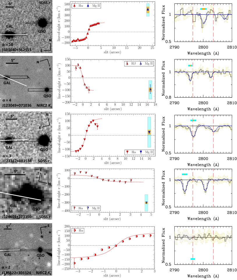
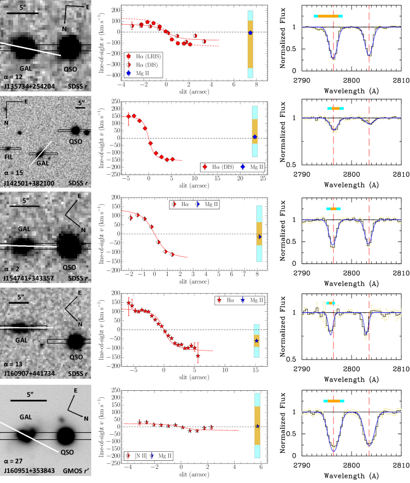
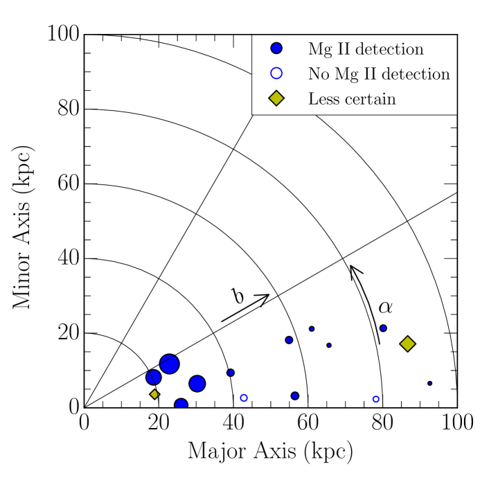
We detected Mg II absorption in 13 of the 15 quasar sightlines. Most of these sightlines probe the CGM of isolated galaxies. Figure 4 illustrates the location and strength of the absorption relative to the major axis. The strongest absorber is the merger, J160951+353838.

Throughout the manuscript, the yellow diamonds identify two systems with uncertain host galaxy assignments. The J091954+291408 sightline intersects a group, see Section 2.4.2, and our spectrum detects two absorption systems. The statistical relationships between absorber and galaxy properties (Lan et al., 2014) suggest that our target has a 50% chance of being the source of either system. The bright, red galaxy and our target have essentially the same impact parameter ( $b=88$ kpc), and red and blue galaxies are equally likely to produce the measured absorption strengths ( $W_{r}(2796)=0.52$ and 0.22 Å). We assign the stronger system to the blue galaxy (our target) and flag the weaker system as potentially mis-assigned, i.e., not produced by our target. We also flag the J124601+173156 sightline through the richer group that includes galaxy J124601+173152. Bordoloi et al. (2011) found that overlap of the circumgalactic media of group galaxies flattens the radial decline in absorption strength. This sightline intersects our target galaxy at $0.14r_{vir}$ , and the contribution from the CGM of the other likely members (at $r>0.70r_{vir}$ ) is likely small. Our primary concern is the object between the quasar and the target galaxy. SDSS DR9 classifies this object as a star. We have yet to spectroscopically verify its stellar nature, and an identification as a compact galaxy would change our interpretation.

3.1. Evidence for Rotation

We explore the connection between the CGM kinematics and the angular momentum vector of the galactic disk. We detect 14 Mg II systems in 13 sightlines. We exclude the two flagged systems. Since only one of the two systems along the J091954+291408 sightline is excluded, 12 systems in 12 sightlines remain in our analysis. Among these 12 sightlines, the Doppler shift of the Mg II absorption is offset more than 20 km s^-1 from the galaxy velocity in eight sightlines. Inspection of Figure 1 shows that the sign of the Mg II Doppler shift always matches the sign of the galactic rotation on the quasar side of the major axis.

Contrast this result with expections for clouds on random orbits in a spherical halo. The shot noise from individual clouds would align the Doppler shifts half the time and produce anti-alignments in all other sightlines. Taking the probability of alignment in any one sightline as $p=0.50$ , the chance of finding eight alignments among 12 sightlines is just 12%.

Consideration of the systems without a net Doppler shift further lowers the odds of obtaining our data from a random, spherical cloud distribution. Our measurement errors on the systemic velocities for four systems – J135734+254204, J142501+382100, J15471+343357, and J160951+352843 – are comparable to the uncertainties in the net Doppler shift of the Mg II absorption. It seems unlikely that higher S/N ratio data would reveal anti-correlations in all four of these systems. The true number of (projected) angular momentum alignments among our 12 sightlines very likely exceeds eight.

Our work was motivated in part by the pioneering study of Steidel et al. (2002) who published rotation curves for the hosts of five Mg II absorbers at $z\approx 0.5$ . Three of their systems had azimuthal angles and disk inclinations consistent with our selection critiera, and the Doppler shifts of all three of these Mg II systems share the sign of the galactic rotation. With alignments now detected in 11 of our combined 15 sightlines, we can conclude that the circumgalactic gas clouds do not follow random orbits. The data require a component of angular momentum that appears to be aligned with the gas disk of the galaxy. A qualitatively similar trend, though quantitatively less significant, has also been seen at larger azimuthal angles (Kacprzak et al., 2010, 2011); and we will quantify the dependence on azimuthal angle in future work.

3.2. Comparison to Galaxy Masses

In our study, the absorption systems span a very broad velocity range compared to the thermal line width. We interpret the broad line widths as evidence that many clouds contribute to each absorption system. The resulting picture requires a population of clouds to produce each Mg II system. If the circumgalactic clouds follow random orbits in a roughly spherical halo, for example, then the line widths would reflect the depth of the gravitational potential while the Doppler shifts would be near the systemic velocity. The shot noise resulting from the finite number of clouds could produce net Doppler shifts along single sightlines, but no average shift would be measured.

To compare the velocity range of the Mg II absorption to the motion of clouds in virial equilibrium, we estimated the halo mass and virial radius of each galaxy. We adopted a stellar mass–halo mass relation derived from abundance matching by Behroozi et al. (2010, hereafter B10). We obtained a median halo mass of $\log(M_{vir}/M_{\odot})=11.51$ , which is significantly lower than the canonical quenching mass of $10^{12}$ ${\rm~{}M_{\odot}}$ (Conroy & Wechsler, 2009; Yang et al., 2012; Kravtsov et al., 2014). We note that the scatter of individual galaxies around the mean stellar mass–halo mass relation introduces an uncertainty of $\pm 0.30$ dex on any single halo mass estimate. This error is in addition to the statistical errors listed in Table 4.

We define the virial radius for each halo by

r_{vir}=M_{vir}(z)^{1/3}\left(\frac{4\pi}{3}\Delta_{vir}(z)\rho_{c}(z)\right)^{-1/3}~{}.

(3)

The B10 definition of the virial mass follows Bryan & Norman (1998) who define the overdensity $\Delta_{vir}(z)$ with respect to the critical density at redshift $z$ by the expression

	$\displaystyle\Delta_{vir}$	$\displaystyle=18\pi^{2}+82x-39x^{2}~{},$		(4)
	$\displaystyle x=\Omega(z)-1$	$\displaystyle\quad\textrm{and}\quad\Omega(z)=\rho_{m}(z)/\rho_{c}(z)~{},$		(5)

where $\rho_{m}(z)$ and $\rho_{c}(z)$ are the mean matter density and critical density at redshift $z$ . For example, $\Delta_{vir}\approx 119$ at $z=0.2$ ( $\Delta_{vir}\approx 273$ with respect to mean matter density). We list estimates of $r_{vir}$ for individual galaxies in Table 4. The median halo virial radius for the 15 galaxies is 160 kpc, and the quasar sightlines intersect the CGM at impact parameters of 0.1–0.5 $r_{vir}$ .

The line-of-sight velocity dispersion through a halo of specified $M_{vir}$ and $r_{vir}$ depends on the mass distribution. In this section, for simplicity, we describe the halo profile as a singular isothermal sphere truncated at the virial radius $r_{vir}$ . The resulting halo circular velocity,

V_{c,vir}=\sqrt{GM_{vir}(r_{vir})/r_{vir}},

(6)

stays constant with radius. In virial equilibrium, the 3D velocity dispersion of the gas clouds would be $\langle v^{2}\rangle=3kT/(\mu m_{H})$ . We adopt the isotropic velocity dispersion in one dimension,

\sigma_{v}^{2}=\frac{\langle v^{2}\rangle}{3}=\frac{V_{c,vir}^{2}}{2}

(7)

as our estimate of the line-of-sight velocity dispersion along the quasar sightline.

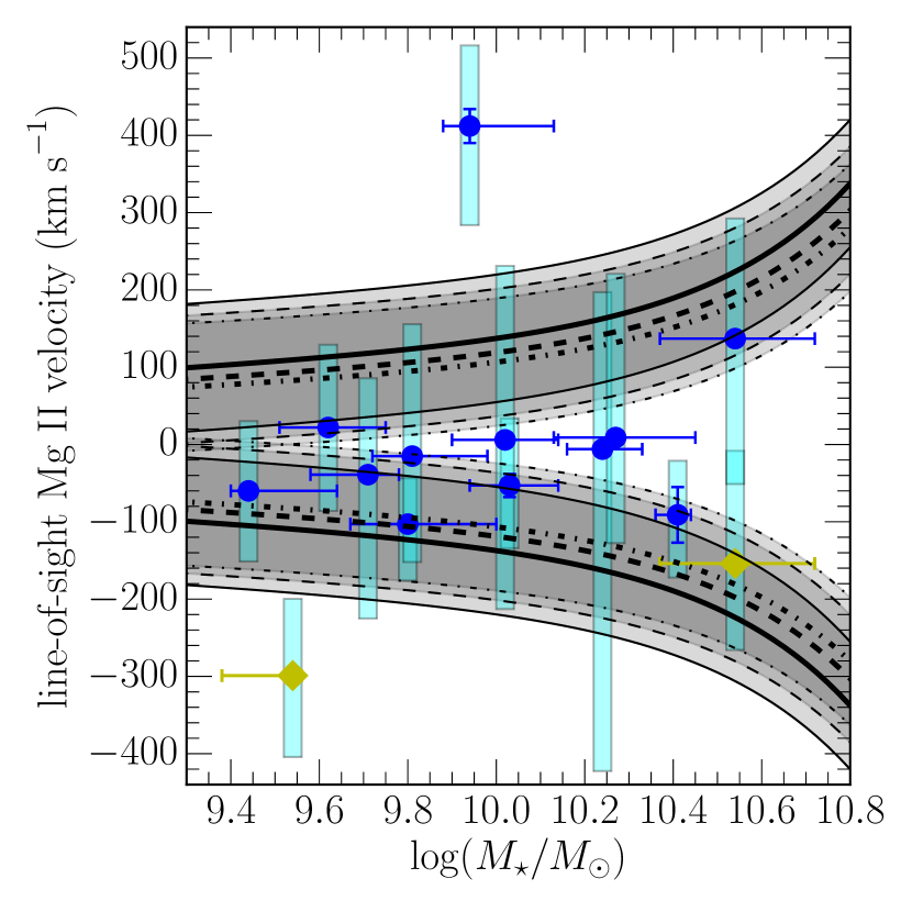
Figure 5 illustrates the velocity dispersion of the Mg II systems over the mass range of our sample. Except for the J103640+565125 sightline and the two systems already flagged as potentially associated with galaxies other than our primary target, the velocity spread of the Mg II absorption along each of the other 11 sightlines is similar to the range predicted for clouds in virial equilibrium. In virial equilibrium, we would also expect the velocity range to broaden with increasing halo mass, and the data do not contradict this expectation.

Our results probe a relatively small range in halo and galaxy properties, but we find no contradictions to virial equilibrium in this regime. In contrast, absorber–galaxy cross-correlation studies have reported an inverse correlation between absorber strength (i.e., velocity width) and the mean halo mass (Bouché et al., 2006; Gauthier et al., 2009), prompting much discussion regarding the virialization of the clouds making up Mg II systems (Bouché et al., 2006; Chen et al., 2010; Tinker & Chen, 2010). We note only that a more recent analysis of absorber–galaxy catalogs shows there is no anti-correlation between Mg II equivalent width and virial mass (Churchill et al., 2013).

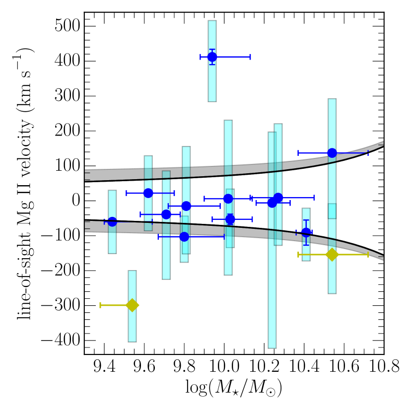
Figure 6 compares the velocity width of the absorption troughs to the halo escape velocity, $v_{esc}(r)=\sqrt{2|\Phi(r)|}$ . The gravitational potential of the halo, $\Phi(r)$ , has been calculated for the isothermal halo profiles at three radii chosen to span our range of the sightline impact parameter. Clearly, the Doppler shifts of the low-ionization-state absorption indicate that the clouds are expected to be bound to the halos. We add that directly matching the projected distance of each sightline with the escape velocity curves is a conservative comparison because the larger galactocentric radius of the cloud in 3D places it in a region of the halo with lower escape velocity, $v_{esc}(r_{3D})<v_{esc}(b)$ .

3.3. The Covering Fraction of Low-ionization-state Gas

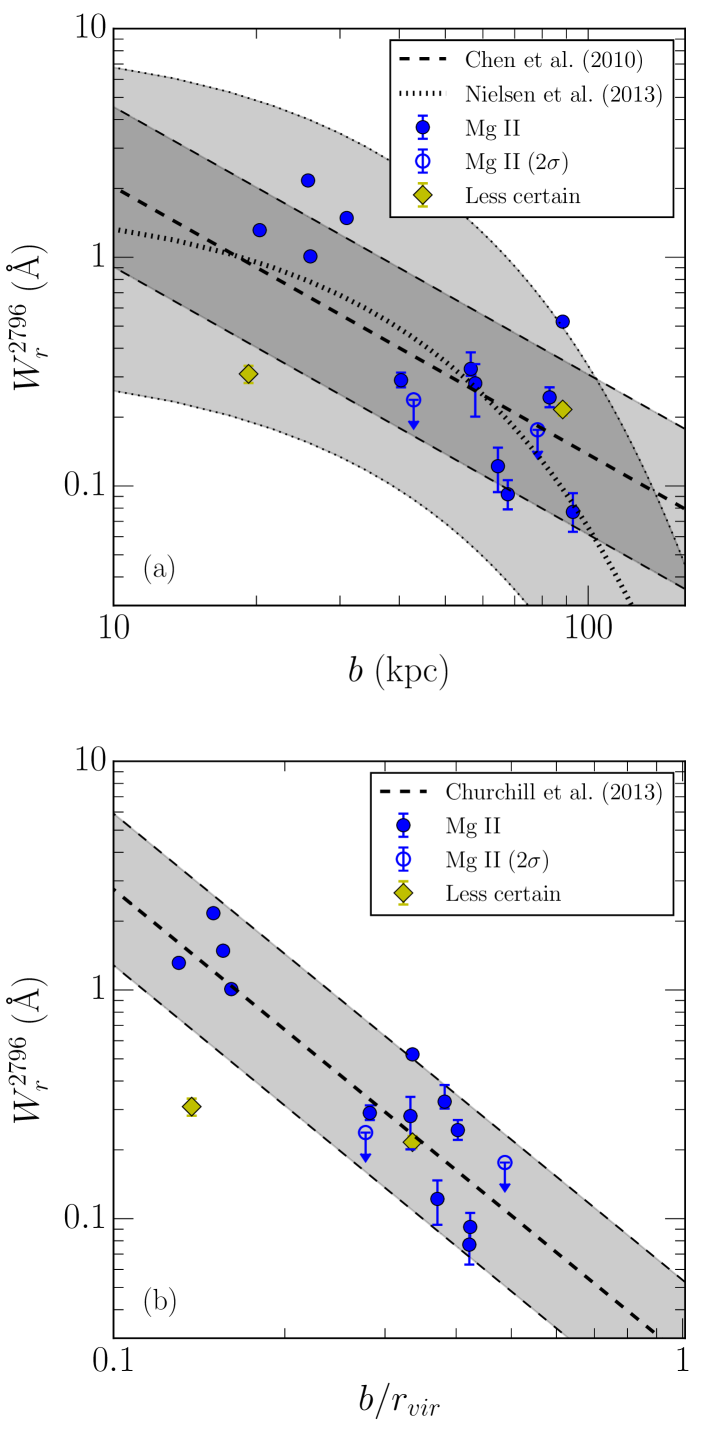
Of the 15 sightlines, seven show strong absorption, $W_{r}(\lambda 2796)\geq 0.3$ Å (Nestor et al., 2005). Since all of our sightlines would easily detect strong absorption, one could claim a covering fraction close to 50%. However, the absorption strengths decrease with impact parameter, following a well-known trend illustrated in Figure 7(a). Our covering fraction measurement accounts for both this radial trend and size differences among the host galaxies. In Figure 7(b), we normalize the impact parameter by the halo virial radius. The strength of the detected absorption is typical for the impact parameters.

Figure 7 shows upper limits for the two non-detections. Since these upper limits fall within a standard deviation of the mean relation, we cannot exclude typical Mg II absorption along these sightlines. Our results are therefore consistent with a unity covering fraction. This high major-axis covering fraction applies to the inner CGM. Our largest impact parameters are 83 kpc (0.24 Å, J142501+382100) and 93 kpc (0.08 Å, J123049+071036).

4. Discussion: Circumgalactic Gas Dynamics

We established in Section 3 that our Mg II detections probe circumgalactic gas largely in virial equilibrium with the target galaxies. However, the orbits of these gas clouds are not random, rather their Doppler shifts show a positive correlation with the sign of each galactic rotation curve.

These kinematic properties of the CGM appear to be consistent with several decades of published literature on intervening absorption systems. For example, surveys of quasar fields traced intervening Mg II absorption to the halos of bright ( $0.7L^{*}_{B}$ ) galaxies at intermediate redshifts, e.g., Steidel et al. (1994). However, a deeper understanding of profile widths and their notable asymmetries (Lanzetta & Bowen, 1992) generated debate between proponents of extended disk models (Prochaska & Wolfe, 1997) and those favoring more spherical halos (McDonald & Miralda-Escudé, 1999). As it turned out, adding a rotational component to the population of clouds proved to be the key to describing the statistical properties of the Mg II line profiles. This solution, however, did not distinguish between rotating disks, halos, or hybrid descriptions (Charlton & Churchill, 1998).

Our selection criteria – specifically (1) inclined disks, (2) low azimuthal angles for the sightlines, and (3) low impact parameters – clearly favor the detection of extended disks. Thus, rather than re-visiting the disk vs. spheroid quandary with a small number of sightlines, we simply explore the conjecture that major-axis sightlines primarily select gas clouds in the extended plane of galactic disks. In this section, we further explore the relationship between the angular momentum of circumgalactic gas and galactic disks.

Our discussion focuses on the measured velocity range and centroid of Mg II absorption in 11 CGM sightlines. We assume that J091954+291345 produces the stronger of the two components in the J091954+291408 sightline and predict that one of the neighboring galaxies in the field will turn out to have a redshift closer to that of the weaker absorption component. We exclude the flagged J124601+173156 sightline from the discussion in this section because the Mg II absorption appears to be associated with a galaxy at smaller angular separation from the quasar than our target galaxy. We defer discussion of the J103640+565125 sightline until we obtain high-resolution imaging because the other targets with such high velocity components have turned out to be groups or mergers. We also note evidence for a galaxy interaction with J160951+353838, which may be related to the unusually broad and strong absorption.

4.1. Angular Momentum of Circumgalactic Gas

Our observations do not directly determine the location of the clouds along each sightline. To gain insight about their relationship to the galaxy, we consider the conjecture that the clouds populate the extended plane of the galactic disk, calculate their implied galactocentric radius and circular velocity, and then examine the implications for the dynamical state of the gas.

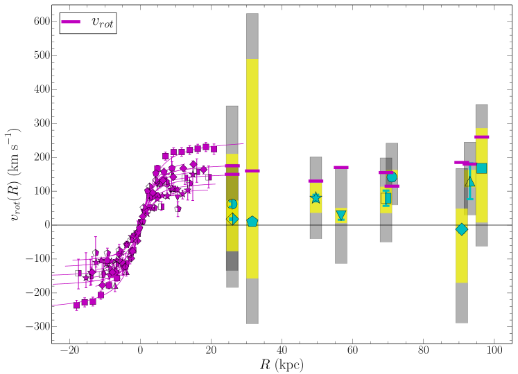
Figure 8 compares the implied rotation speed of the Mg II systems to the rotation speed of the galactic disk. As described in Section 4.1, the Doppler shifts of the Mg II systems share the sign of the galactic rotation along seven sightlines. The measurement errors for four systems are consistent with no net Doppler shift, and these systems have substantial equivalent width on both sides of the systemic velocity. The range of deprojected Mg II velocities often reaches the asymptotic rotation speed of the disk. The Doppler shift of most of the absorption equivalent width is, however, too low to be consistent with purely circular orbits in a disk.

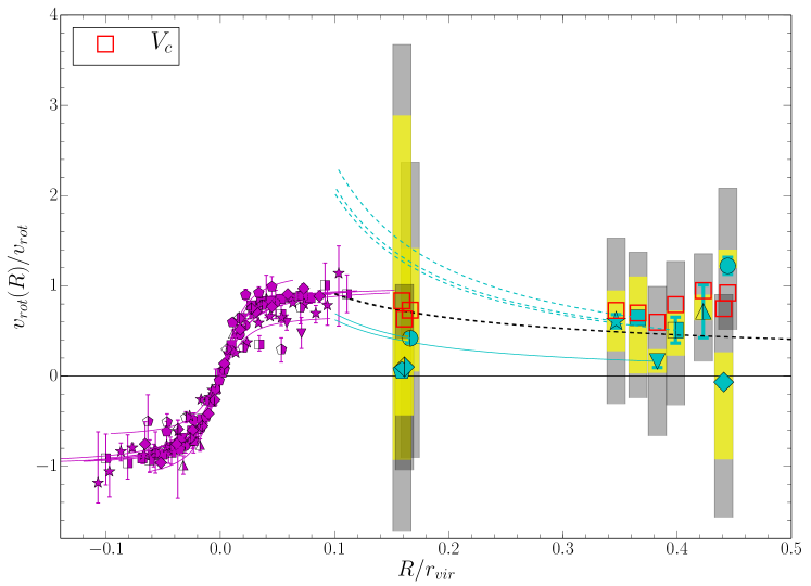
In Figure 9, we have normalized the galaxy rotation curves by the asymptotic rotation speed, $v_{rot}$ , of each galaxy. The red squares show the halo circular velocity assuming a Navarro, Frenk, and White (NFW; Navarro et al. 1996) halo profile with the concentration parameter $c(z,M_{vir})$ calculated using the python package Colossus introduced by Diemer & Kravtsov (2015).⁹⁹9 Diemer & Kravtsov (2015, hereafter DK15) adopt $M_{200c}$ to describe a halo with a mean density 200 times the critical density and model the corresponding concentration parameter $c_{200c}$ , but Behroozi et al. (2010) define halo mass differently. Colossus provides the conversion of halo concentration between different mass definitions, for which the discussion in Appendix C of DK15 suggests that the inaccuracies of these conversions are no more than $\sim$ 20%. The halo circular velocity resembles the form of Equation (6) but with a radial dependence,

V_{c}(r)=\sqrt{GM_{vir}(r)/r}.

(8)

Most of the Mg II equivalent width is detected at Doppler shifts less than that generated by clouds on circular orbits. The velocity widths of the systems are broad enough to include gas on a circular orbit, but the estimated speed of a circular orbit exceeds the centroid velocity (cyan symbols in Figure 9). Adding the stellar mass from Table 4 to the halo mass raises the circular velocity slightly (2 - 6%) and increases the magnitude of the discrepancy. Only the sightline probing the CGM at the largest radius provides an exception. At $R/r_{vir}\approx 0.45$ , the J084723+254105 sightline has a Doppler shift larger than expected from circular orbits.

If clouds near the disk plane with $R/r_{vir}\lesssim 0.45$ are not fully described by circular orbits, then what can we say about their dynamical state? Since we have shown that the velocity spread of the systems is consistent with virial motion, we can conclude that the clouds have a significant velocity component that is perpendicular to any tangential motion in the disk plane. We suggest radial inflow as a physically likely origin for this extra velocity component. While the spectral line profiles do not uniquely distinguish radial inflow from other velocity vectors, we argue that our selection of major-axis sightlines favors this solution.

If our interpretation is correct, then it has implications for how galaxies get their gas. We illustrate where the infalling gas might obtain a circular orbit by drawing curves of constant angular momentum in Figure 9. By following these curves, we see that some of the gas detected in Mg II absorption has specific angular momentum comparable to the galactic disk. The broad line widths, however, indicate that other clouds might obtain circular orbits at radii several times that of the visible galactic disk. Large gas disks have been detected in H I 21 cm observations of nearby spiral galaxies. If we have detected extended gas disks at $z\approx 0.2$ , then the composition of the gas is clearly not pristine implying significant metal recycling.

4.2. The Tension between the Velocity Widths of Mg II Absorbers and Rotating Disks

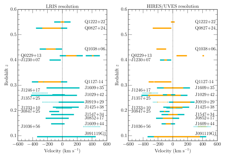
Figure 10 illustrates the velocity spread of our Mg II absorption troughs relative to the systemic velocities of the associated galaxies. We have added published observations of sightlines with $\alpha\leq 30\mbox{${}^{\circ}$}$ near inclined, star-forming galaxies. We do not include sightlines from the COS Halos survey (Tumlinson et al., 2011, 2013; Werk et al., 2013, 2014) because no measurements of galaxy rotation have been published. As introduced in Section 4.1, three sightlines from Steidel et al. (2002, hereafter S02) satisfy our selection criteria. At intermediate redshifts, we add two sightlines from Kacprzak et al. (2010, hereafter K10); and, at lower redshift, we found one sightline from Kacprzak et al. (2011, hereafter K11). Little data of this type exists at higher redshifts, but two ground-breaking papers suggest that similar trends may be present in the low-ionization-state absorption. Just 20^∘ off the major axis of a $z=2.3283$ galaxy, Bouché et al. (2013) detected absorption from low ions (but did not cover Mg II) at an impact parameter of 26 kpc. The Doppler shift of the main absorption component is 180 km s^-1 and in the same direction as the galactic rotation, whereas the total absorption spans from $-35$ km s^-1 to $+300$ km s^-1. Just 12 kpc from a $z=0.9096$ galaxy, Bouché et al. (2016) resolve the Mg II line profile in a sightline 15^∘ off the major axis. The Doppler shift is again in the same sense as the galaxy rotation, and the velocities range from $-230$ km s^-1 to $+265$ km s^-1.

Differences in instrumental resolution among these observations affect the measured velocity widths of the absorption troughs. We have attempted to correct all observations to the same effective resolution in Figure 10. In the left panel of Figure 10, we have simply degraded the spectra of bright quasars taken using Keck/HIRES or VLT/UVES ( $v_{\mathrm{res}}\simeq 6$ km s^-1) to our resolution by convolving with the LRIS line-spread function. The inverse process – recovering the intrinsic velocity width of a system from our lower resolution spectra – is inherently more noisy. We show the results of this exercise in the right panel of Figure 10. The observations reported by K11 were also obtained with Keck/LRIS at a spectral resolution ( $v_{\mathrm{res}}\simeq 155$ km s^-1) similar to our median resolution. Section 4.1 of the K11 paper convincingly argues that these LRIS line widths should be decreased by 85 km s^-1 on both sides before they are compared to well resolved line profiles. We have confirmed that simply fitting the Mg II absorption with a Gaussian profile convolved with the LRIS line spread gives a consistent velocity width. After taking instrumental broadening into account, we find that four of our 11 systems show absorptions at velocities on both sides of the galaxy systemic velocity.

A dynamical description of the low-ionization-state gas kinematics must explain the following: (1) the correlation of the sign of the net Doppler shift with the galactic disk, (2) the broad line width, and (3) the generation of absorption on both sides of the systemic velocity. The simple disk model naturally satisfies the first criterion, but the other kinematic properties prove challenging to explain with the simple disk picture. For individual systems, we have explored two types of solutions: (1) adding a vertical velocity gradient to the disk rotation speed and (2) adding radial infall in the disk plane. We provide a mathematical description of these models in the Appendix. The solution space is highly degenerate. Rather than presenting every possible solution, we focus on answering a few well posed questions.

4.2.1 Are There Sightlines that cannot be Fitted by Disk Rotation?

Disk rotation can never produce a sign change in the line-of-sight velocity along a sightline. Equation (A4) and diagrams in the Appendix demonstrate this fact quantitatively.¹⁰¹⁰10 Poor spectral resolution could certainly smear the line profile so that it crossed the systemic velocity. In principle, turbulence could provide a physical mechanism to accomplish this line broadening, but requiring turbulent velocities comparable to the circular velocity implies a structure that cannot really be labeled a disk.

We find four sightlines with absorption on both sides of the systemic velocity – J135734+254204, J142501+382100, J154741+343357, and J160951+353843, so the simple disk model cannot describe the velocity range of the Mg II absorption. The spherical halo model adequately describes these systems, and these sightlines need not intersect a disk at all. Nonetheless, we asked whether an extended disk with radial inflow provided a viable alternative explanation of the line widths. We found that inflow ( $v_{R}=-250$ km s^-1) in a thick disk ( $2H_{\mathrm{eff}}=40$ kpc) produces the velocity range of the J142501+382100 system. The other three systems required thicker disks and higher inflow speeds. The extreme values of these parameters lead us to conclude that extended disks are not a viable model for these systems.

For the systems with single-sided absorption, a rotating disk can describe the velocity range measured in five of the seven sightlines, albeit with a troubling implication. Recall that in Figure 10, the instrinsic line widths typically span around a hundred km s^-1 or more. The problem is that the pathlength of a sightline through a thin disk is just the vertical thickness of the disk, $2H_{\mathrm{eff}}$ (as illustrated in the schematic diagrams in the Appendix), lengthened by the secant of the viewing angle. Unless we view the disk exactly edge-on, the intercepted velocity range will be small. we found that the simple disk model required disk thicknesses of the order of the virial radius – i.e., tall rotating cylinders rather than disks.

As demonstrated in S02 and in the Appendix, adding a scale-height $h_{v}$ for the vertical velocity gradient such that the disk rotation speed decreases with increasing perpendicular distance from the disk midplane will bring the line-of-sight velocity $v_{los}$ toward zero over a shorter pathlength along the sightline. As a fiducial reference point, we adopted $h_{v}=10$ kpc. For our measured range of rotation speeds, this choice of velocity scale height produces a vertical gradient between 11 and 26 km s^-1 per kpc. Above the plane of nearby spiral galaxies, the rotation lags the disk; our adopted $h_{v}$ creates a vertical velocity gradient consistent with measurements of $dv_{\phi}/dz=-8{\rm~{}to~{}}-60$ km s^-1 per kpc (Oosterloo et al., 2007; Heald et al., 2011; Marasco & Fraternali, 2011; Zschaechner et al., 2011, 2012; Gentile et al., 2013; Kamphuis et al., 2013; Zschaechner & Rand, 2015). With this velocity gradient in the extraplanar gas, we found solutions with very thick disks and reduced the median $H_{\mathrm{eff}}$ to 20 kpc (for the models fitted to the five disks).¹¹¹¹11 The total vertical thickness of the disk is $2H_{\mathrm{eff}}$ ; $H_{\mathrm{eff}}$ measures the disk thickness from the disk midplane. We also found an alternative picture, however, which appears at least as plausible in our opinion. When a radial inflow component was allowed, the median $H_{\mathrm{eff}}$ dropped to 10 kpc, and the range of inflow speed ranged from 40 to 180 km s^-1.

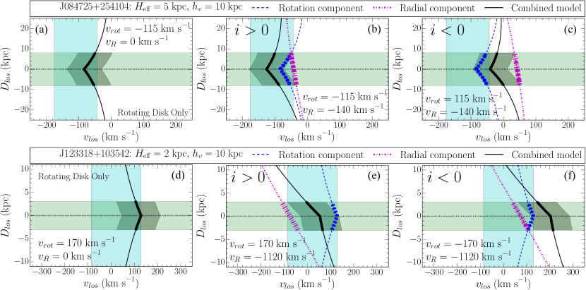
Figure 11 illustrates the failure of the thick disk model for the other two Mg II detections. The thick disk model cannot describe the J084723+254105 system because the large blueshift of the absorption exceeds the projected rotation speed ( $v_{rot}\sin i=115\mbox{~{}km~{}s${}^{-1}$}\ \sin(52\mbox{${}^{\circ}$})=91\mbox{~{}km~{}s${}^{-1}$}$ ). The bottom row of Figure 11 illustrates a slightly different mode of failure for the thick disk model. Toward the sightline associated with J123318+103542, the absorption velocities do not reach the projected circular velocity of the galactic disk. In the center panels of Figure 11, we successfully fit these two systems by introducing radial infall in the disk plane. The observed line-of-sight velocities are the projection of the total velocity vector produced by the addition of rotation and inflow in the disk plane. Whether the infall boosts or cancels the projected circular velocity depends on geometry. The Appendix clearly illustrates the origin of this asymmetry; we could not find it described previously in the literature. This solution has a reasonable disk of thickness $H_{\mathrm{eff}}=5$ kpc and $H_{\mathrm{eff}}=2$ kpc, with the velocity scale height $h_{v}=10$ kpc in the models for J084725+254104 and J123318+103542 respectively. The corresponding inflow speeds are $v_{R}=-140$ km s^-1 and $v_{R}=-1120$ km s^-1 in the two models.

4.2.2 Is Radial Inflow Excluded When it is not Required?

A rotating disk with radial infall provides a plausible description of the Mg II kinematics in our two systems that cannot be fit with simpler models. While the other systems do allow simpler descriptions, we emphasize that the implied parameters generate tension with our expectations for real disks. Without inflow, the five systems described by rotating disks require very thick disks, and we suggest solutions with thinner disks and inflow as a viable alternative. The same picture, inflow in a rotating gas disk, can reproduce broad absorption centered near the systemic velocity. We do not favor this interpretation for those four sightlines because simpler models remain consistent with our observations; we simply emphasize that, no, we do not exclude this interpretation for a single sightline.

4.3. Implications for How Galactic Disks Get Their Gas

The gas flows in simulations of galaxy formation motivated us to consider the observational signature of gas flows near the plane of the galactic disk. We observed the CGM along sightlines near the galactic major axis in an effort to select such disks if they exist. We demonstrated that this circumgalactic gas has a component of angular momentum in the same direction as the disk angular momentum. If the gas clouds follow circular orbits in the extended plane of the galactic disk, however, their Doppler shifts would be larger than observed. One interpretation of this result is simply that the angular momentum vector of the inner circumgalactic gas is only partially aligned with that of the disk. We suggest, however, that radial inflow in the disk plane provides another viable description of the observations.

The inferred mass flux depends directly on the column density. Since we generally obtained a very conservative lower limit on the column density, we estimate a lower limit of the mass flux. For purposes of illustration, we use solar metallicity (Morton, 2003) and a unity ionization fraction of singly ionized magnesium, i.e., $N(\mathrm{Mg}^{+})/N(\mathrm{Mg})=1$ .¹²¹²12 The ionization fraction $N(\mathrm{Mg}^{+})/N(\mathrm{Mg})$ varies between 0.1 and 1(Murray et al., 2007; Martin et al., 2012). Substituting the lower limits from Table 3, we infer hydrogen columns from $6\times 10^{16}$ cm^-2 to $3\times 10^{18}$ cm^-2. We apply Equation (1) from Bouché et al. (2013). For the two systems that require inflow, the mass flux exceeds 0.07–1 $~{}{\rm M_{\odot}}$ yr^-1. If we interpret the five systems with single-sided absorption as inflow detections, then the mass fluxes are at least 0.02–0.08 $~{}{\rm M_{\odot}}$ yr^-1. In general, the true mass flux could be much, much larger; but we will need higher resolution spectra to produce accurate measurements.

In the context of this inflow picture, the new observations place some constraints on how galaxies get their gas. First, the inflow speeds we found were generally within a factor of two of the rotation speed. One sightline, quasar J123317+103538 associated with galaxy J123318+103542, required a much larger inflow velocity to cancel the tangential velocity. We remain skeptical of inflow velocities as large as 1000 km s^-1; however, some high velocity clouds have velocities this large relative to the Local Standard of Rest (Wakker & van Woerden, 1997). Second, in Figure 9, we sketched curves of constant $RV(R)$ and then argued that some of the infalling gas would have to reach the galactic disk. Possible strategies for testing this picture include the following: (1) confirming/refuting the predictions for the disk inclination and spiral arm morphology, (2) examining the implications of the model for a broader range of azimuthal angles, and (3) significantly increasing the sample of major-axis sightlines.

Given the absence of previous evidence for gas inflow in galactic disks, this result if verified would have significant implications for how galactic disks get their gas. In this context, it is interesting to compare the galaxies in our sample to a younger version of the MW galaxy in the past. We use the stellar mass evolution function presented in van Dokkum et al. (2013). They study galaxies at different redshifts with the same rank order in stellar mass as the MW at $z=0$ , and adopt the stellar mass of the present-day MW as around $5\times 10^{10}M_{\odot}$ , i.e., $\log(M_{\star}/M_{\odot})=10.70$ (Flynn et al., 2006; McMillan, 2011). They then associate galaxies at different redshifts by requiring them to have the same cumulative comoving number density. We use their approximate stellar mass evolution function

\log({M_{\star\textrm{,MW}}/M_{\odot}})=10.7-0.045z-0.13z^{2}

(9)

to find the predicted stellar mass of the MW progenitors at $z=0.2$ as $\log({M_{\star\textrm{,MW}}/M_{\odot}})_{z=0.2}=10.69$ , which is marginally lower than that at $z=0$ . This predicted stellar mass has an uncertainty of $\sim$ 0.2 dex. The comparison between our galaxy sample at $z=0.2$ and the MW progenitors at $z=0.2$ show that our median galaxy is 0.87 dex less massive than the typical MW progenitor 2.5 Gyr ago; but the upper mass range of our sample is consistent with the expected masses of MW progenitors.

5. Conclusion

We presented new observations of 15 galaxy–quasar pairs. This study more than doubles the number of quasar sightlines studied within $30^{\mathrm{o}}$ of the major axis of star-forming galaxies. The focus on typical, star-forming galaxies allows us to consider the ensemble of sightlines as multiple sightlines through the same average CGM.

Gas clouds in the plane of these galactic disks are a plausible source of Mg II absorption detected in the quasar spectrum near the redshift of the foreground galaxy. Models predict that such gas has been accreted recently. We therefore asked the question of whether the gas kinematics might yield signs of accretion.

We detected Mg II absorption in 13 sightlines with $W_{r}(\lambda 2796)\gtrsim 0.1$ Å. The sign of the Doppler shifts of these systems always matched the sign of the galactic rotation on the quasar side of the major axis. This result demonstrated that the motion of the absorbing gas is not random. The observations do not require the absorbing clouds to be located in the plane of the galactic disk, but we focused our modeling effort on gas in an extended plane for two reasons: (1) these models offer the simplest geometry allowed by the data, and (2) numerical simulations of individual galaxies predict that gas accreted at late times feeds an extended gas disk. The Doppler shifts of the Mg II systems are less than expected for gas on circular orbits. If these clouds reside in the disk plane, then they will spiral inwards through the disk. This inflow mechanism would broaden the absorption troughs.

The velocity widths of the Mg II systems typically agree with expectations for gas in virial equilibrium. Host galaxy mis-assignments plausibly explain the outliers. However, the velocity range poses a challenge for simple models. The velocity widths of two Mg II systems cannot be fit by a thick rotating disk model. Furthermore, modeling the widths of many systems requires the disk to be ridiculously thick, essentially morphing into a rotating cylinder that is much thicker than the disk radius.

We found that radial infall in the disk plane solves the above dilemmas. Other solutions may exist, but we argue that radial infall is the simplest geometry consistent with the data. These measurements provide a benchmark against which the accuracy of the gas accretion process in numerical simulations should be evaluated. Our future work will address how the circumgalactic gas kinematics depend on azimuthal angle.

This research was partially supported by the National Science Foundation under AST-1109288. G.G.K. acknowledges the support of the Australian Research Council through the award of a Future Fellowship (FT140100933). We thank the referee for the useful suggestions. We thank Mark Seibert for the discussion on GALEX photometry. We gratefully acknowledge conversations with Peng Oh and Andrey Kravtsov, which contributed to shaping our interpretation of these data. Most of the data presented herein were obtained at the W.M. Keck Observatory, which is operated as a scientific partnership among the California Institute of Technology, the University of California and the National Aeronautics and Space Administration. The Observatory was made possible by the generous financial support of the W.M. Keck Foundation. The authors wish to recognize and acknowledge the very significant cultural role and reverence that the summit of Mauna Kea has always had within the indigenous Hawaiian community. We are most fortunate to have the opportunity to conduct observations from this mountain. Some presented data are based on observations obtained with the Apache Point Observatory 3.5 m telescope, which is owned and operated by the Astrophysical Research Consortium.
Facilities: Keck:I (LRIS), Keck:II (NIRC2), Gemini:Gillett (GMOS), GALEX, ARC

References

Ahn et al. (2012) Ahn, C. P., Alexandroff, R., Allende Prieto, C., et al. 2012, ApJS, 203, 21
Behroozi et al. (2010) Behroozi, P. S., Conroy, C., & Wechsler, R. H. 2010, ApJ, 717, 379
Benjamin (2002) Benjamin, R. A. 2002, in Astronomical Society of the Pacific Conference Series, Vol. 276, Seeing Through the Dust: The Detection of HI and the Exploration of the ISM in Galaxies, ed. A. R. Taylor, T. L. Landecker, & A. G. Willis, 201
Benjamin (2012) Benjamin, R. A. 2012, in EAS Publications Series, Vol. 56, EAS Publications Series, ed. M. A. de Avillez, 299–304
Blanton et al. (2003) Blanton, M. R., Hogg, D. W., Bahcall, N. A., et al. 2003, ApJ, 592, 819
Boksenberg & Sargent (2015) Boksenberg, A., & Sargent, W. L. W. 2015, ApJS, 218, 7
Bordoloi et al. (2014) Bordoloi, R., Lilly, S. J., Kacprzak, G. G., & Churchill, C. W. 2014, ApJ, 784, 108
Bordoloi et al. (2011) Bordoloi, R., Lilly, S. J., Knobel, C., et al. 2011, ApJ, 743, 10
Bouché et al. (2012) Bouché, N., Hohensee, W., Vargas, R., et al. 2012, MNRAS, 426, 801
Bouché et al. (2013) Bouché, N., Murphy, M. T., Kacprzak, G. G., et al. 2013, Science, 341, 50
Bouché et al. (2006) Bouché, N., Murphy, M. T., Péroux, C., Csabai, I., & Wild, V. 2006, MNRAS, 371, 495
Bouché et al. (2010) Bouché, N., Dekel, A., Genzel, R., et al. 2010, ApJ, 718, 1001
Bouché et al. (2016) Bouché, N., Finley, H., Schroetter, I., et al. 2016, ApJ, 820, 121
Brook et al. (2012) Brook, C. B., Stinson, G., Gibson, B. K., Wadsley, J., & Quinn, T. 2012, MNRAS, 424, 1275
Bruzual & Charlot (2003) Bruzual, G., & Charlot, S. 2003, MNRAS, 344, 1000
Bryan & Norman (1998) Bryan, G. L., & Norman, M. L. 1998, ApJ, 495, 80
Calzetti et al. (2000) Calzetti, D., Armus, L., Bohlin, R. C., et al. 2000, ApJ, 533, 682
Chabrier (2003) Chabrier, G. 2003, PASP, 115, 763
Charlton & Churchill (1998) Charlton, J. C., & Churchill, C. W. 1998, ApJ, 499, 181
Chen et al. (2010) Chen, H.-W., Helsby, J. E., Gauthier, J.-R., et al. 2010, ApJ, 714, 1521
Chen et al. (2005) Chen, H.-W., Kennicutt, Jr., R. C., & Rauch, M. 2005, ApJ, 620, 703
Christensen et al. (2016) Christensen, C. R., Davé, R., Governato, F., et al. 2016, ApJ, 824, 57
Churchill et al. (2013) Churchill, C. W., Trujillo-Gomez, S., Nielsen, N. M., & Kacprzak, G. G. 2013, ApJ, 779, 87
Conroy & Wechsler (2009) Conroy, C., & Wechsler, R. H. 2009, ApJ, 696, 620
Danovich et al. (2015) Danovich, M., Dekel, A., Hahn, O., Ceverino, D., & Primack, J. 2015, MNRAS, 449, 2087
Danovich et al. (2012) Danovich, M., Dekel, A., Hahn, O., & Teyssier, R. 2012, MNRAS, 422, 1732
Davé et al. (2012) Davé, R., Finlator, K., & Oppenheimer, B. D. 2012, MNRAS, 421, 98
Diamond-Stanic et al. (2016) Diamond-Stanic, A. M., Coil, A. L., Moustakas, J., et al. 2016, ApJ, 824, 24
Diemer & Kravtsov (2015) Diemer, B., & Kravtsov, A. V. 2015, ApJ, 799, 108
Edlén (1966) Edlén, B. 1966, Metrologia, 2, 71
Eisenstein et al. (2011) Eisenstein, D. J., Weinberg, D. H., Agol, E., et al. 2011, AJ, 142, 72
Erb et al. (2012) Erb, D. K., Quider, A. M., Henry, A. L., & Martin, C. L. 2012, ApJ, 759, 26
Fitzpatrick (1999) Fitzpatrick, E. L. 1999, PASP, 111, 63
Flynn et al. (2006) Flynn, C., Holmberg, J., Portinari, L., Fuchs, B., & Jahreiß, H. 2006, MNRAS, 372, 1149
Ford et al. (2014) Ford, A. B., Davé, R., Oppenheimer, B. D., et al. 2014, MNRAS, 444, 1260
Ford et al. (2016) Ford, A. B., Werk, J. K., Davé, R., et al. 2016, MNRAS, 459, 1745
Fox et al. (2014) Fox, A. J., Wakker, B. P., Barger, K. A., et al. 2014, ApJ, 787, 147
Gauthier & Chen (2012) Gauthier, J.-R., & Chen, H.-W. 2012, MNRAS, 424, 1952
Gauthier et al. (2009) Gauthier, J.-R., Chen, H.-W., & Tinker, J. L. 2009, ApJ, 702, 50
Gentile et al. (2013) Gentile, G., Józsa, G. I. G., Serra, P., et al. 2013, A&A, 554, A125
Ghez et al. (2008) Ghez, A. M., Salim, S., Weinberg, N. N., et al. 2008, ApJ, 689, 1044
Hanuschik (2003) Hanuschik, R. W. 2003, A&A, 407, 1157
Heald et al. (2011) Heald, G., Józsa, G., Serra, P., et al. 2011, A&A, 526, A118
Heckman et al. (2000) Heckman, T. M., Lehnert, M. D., Strickland, D. K., & Armus, L. 2000, ApJS, 129, 493
Hubble (1926) Hubble, E. P. 1926, ApJ, 64, 321
Kacprzak et al. (2011) Kacprzak, G. G., Churchill, C. W., Barton, E. J., & Cooke, J. 2011, ApJ, 733, 105
Kacprzak et al. (2010) Kacprzak, G. G., Churchill, C. W., Ceverino, D., et al. 2010, ApJ, 711, 533
Kacprzak et al. (2012) Kacprzak, G. G., Churchill, C. W., & Nielsen, N. M. 2012, ApJ, 760, L7
Kacprzak et al. (2015) Kacprzak, G. G., Muzahid, S., Churchill, C. W., Nielsen, N. M., & Charlton, J. C. 2015, ApJ, 815, 22
Kamphuis et al. (2013) Kamphuis, P., Rand, R. J., Józsa, G. I. G., et al. 2013, MNRAS, 434, 2069
Keeney et al. (2013) Keeney, B. A., Stocke, J. T., Rosenberg, J. L., et al. 2013, ApJ, 765, 27
Kennicutt (1998) Kennicutt, Jr., R. C. 1998, ARA&A, 36, 189
Kravtsov et al. (2014) Kravtsov, A., Vikhlinin, A., & Meshscheryakov, A. 2014, ArXiv e-prints, arXiv:1401.7329
Kriek et al. (2009) Kriek, M., van Dokkum, P. G., Labbé, I., et al. 2009, ApJ, 700, 221
Lan et al. (2014) Lan, T.-W., Ménard, B., & Zhu, G. 2014, ApJ, 795, 31
Lanzetta & Bowen (1992) Lanzetta, K. M., & Bowen, D. V. 1992, ApJ, 391, 48
Lehner et al. (2013) Lehner, N., Howk, J. C., Tripp, T. M., et al. 2013, ApJ, 770, 138
Marasco & Fraternali (2011) Marasco, A., & Fraternali, F. 2011, A&A, 525, A134
Martin et al. (2002) Martin, C. L., Kobulnicky, H. A., & Heckman, T. M. 2002, ApJ, 574, 663
Martin et al. (2012) Martin, C. L., Shapley, A. E., Coil, A. L., et al. 2012, ApJ, 760, 127
Martin et al. (2005) Martin, D. C., Fanson, J., Schiminovich, D., et al. 2005, ApJ, 619, L1
McDonald & Miralda-Escudé (1999) McDonald, P., & Miralda-Escudé, J. 1999, ApJ, 519, 486
McGaugh et al. (2010) McGaugh, S. S., Schombert, J. M., de Blok, W. J. G., & Zagursky, M. J. 2010, ApJ, 708, L14
McMillan (2011) McMillan, P. J. 2011, MNRAS, 414, 2446
Morrissey et al. (2007) Morrissey, P., Conrow, T., Barlow, T. A., et al. 2007, ApJS, 173, 682
Morton (2003) Morton, D. C. 2003, ApJS, 149, 205
Muratov et al. (2015) Muratov, A. L., Kereš, D., Faucher-Giguère, C.-A., et al. 2015, MNRAS, 454, 2691
Murray et al. (2007) Murray, N., Martin, C. L., Quataert, E., & Thompson, T. A. 2007, ApJ, 660, 211
Navarro et al. (1996) Navarro, J. F., Frenk, C. S., & White, S. D. M. 1996, ApJ, 462, 563
Nestor et al. (2005) Nestor, D. B., Turnshek, D. A., & Rao, S. M. 2005, ApJ, 628, 637
Nielsen et al. (2013) Nielsen, N. M., Churchill, C. W., & Kacprzak, G. G. 2013, ApJ, 776, 115
Nielsen et al. (2015) Nielsen, N. M., Churchill, C. W., Kacprzak, G. G., Murphy, M. T., & Evans, J. L. 2015, ApJ, 812, 83
Oke et al. (1995) Oke, J. B., Cohen, J. G., Carr, M., et al. 1995, PASP, 107, 375
Oosterloo et al. (2007) Oosterloo, T., Fraternali, F., & Sancisi, R. 2007, AJ, 134, 1019
Oppenheimer et al. (2010) Oppenheimer, B. D., Davé, R., Kereš, D., et al. 2010, MNRAS, 406, 2325
Phillips et al. (2006) Phillips, A. C., Miller, J., Cowley, D., & Wallace, V. 2006, in Society of Photo-Optical Instrumentation Engineers (SPIE) Conference Series, Vol. 6269, Society of Photo-Optical Instrumentation Engineers (SPIE) Conference Series, 1
Planck Collaboration et al. (2015) Planck Collaboration, Ade, P. A. R., Aghanim, N., et al. 2015, ArXiv e-prints, arXiv:1502.01589
Press et al. (1992) Press, W. H., Teukolsky, S. A., Vetterling, W. T., & Flannery, B. P. 1992, Numerical recipes in FORTRAN. The art of scientific computing
Prochaska & Wolfe (1997) Prochaska, J. X., & Wolfe, A. M. 1997, ApJ, 487, 73
Prochter et al. (2006) Prochter, G. E., Prochaska, J. X., & Burles, S. M. 2006, ApJ, 639, 766
Putman et al. (2012) Putman, M. E., Peek, J. E. G., & Joung, M. R. 2012, ARA&A, 50, 491
Quiret et al. (2016) Quiret, S., Péroux, C., Zafar, T., et al. 2016, MNRAS, 458, 4074
Rockosi et al. (2010) Rockosi, C., Stover, R., Kibrick, R., et al. 2010, in Society of Photo-Optical Instrumentation Engineers (SPIE) Conference Series, Vol. 7735, Society of Photo-Optical Instrumentation Engineers (SPIE) Conference Series, 0
Rubin et al. (2012) Rubin, K. H. R., Prochaska, J. X., Koo, D. C., & Phillips, A. C. 2012, ApJ, 747, L26
Rubin et al. (2014) Rubin, K. H. R., Prochaska, J. X., Koo, D. C., et al. 2014, ApJ, 794, 156
Schlafly & Finkbeiner (2011) Schlafly, E. F., & Finkbeiner, D. P. 2011, ApJ, 737, 103
Shen et al. (2012) Shen, S., Madau, P., Aguirre, A., et al. 2012, ApJ, 760, 50
Shull (2014) Shull, J. M. 2014, ApJ, 784, 142
Sommer-Larsen (1991) Sommer-Larsen, J. 1991, MNRAS, 249, 368
Steidel et al. (1994) Steidel, C. C., Dickinson, M., & Persson, S. E. 1994, ApJ, 437, L75
Steidel et al. (2002) Steidel, C. C., Kollmeier, J. A., Shapley, A. E., et al. 2002, ApJ, 570, 526
Stewart et al. (2013) Stewart, K. R., Brooks, A. M., Bullock, J. S., et al. 2013, ApJ, 769, 74
Stewart et al. (2011) Stewart, K. R., Kaufmann, T., Bullock, J. S., et al. 2011, ApJ, 738, 39
Tinker & Chen (2010) Tinker, J. L., & Chen, H.-W. 2010, ApJ, 709, 1
Tumlinson et al. (2011) Tumlinson, J., Thom, C., Werk, J. K., et al. 2011, Science, 334, 948
Tumlinson et al. (2013) —. 2013, ApJ, 777, 59
van Dam et al. (2006) van Dam, M. A., Bouchez, A. H., Le Mignant, D., et al. 2006, PASP, 118, 310
van den Bergh (1962) van den Bergh, S. 1962, AJ, 67, 486
van Dokkum (2001) van Dokkum, P. G. 2001, PASP, 113, 1420
van Dokkum et al. (2013) van Dokkum, P. G., Leja, J., Nelson, E. J., et al. 2013, ApJ, 771, L35
Veilleux et al. (2005) Veilleux, S., Cecil, G., & Bland-Hawthorn, J. 2005, ARA&A, 43, 769
Wakker & van Woerden (1997) Wakker, B. P., & van Woerden, H. 1997, ARA&A, 35, 217
Wakker et al. (1999) Wakker, B. P., Howk, J. C., Savage, B. D., et al. 1999, Nature, 402, 388
Weiner et al. (2009) Weiner, B. J., Coil, A. L., Prochaska, J. X., et al. 2009, ApJ, 692, 187
Werk et al. (2013) Werk, J. K., Prochaska, J. X., Thom, C., et al. 2013, ApJS, 204, 17
Werk et al. (2014) Werk, J. K., Prochaska, J. X., Tumlinson, J., et al. 2014, ApJ, 792, 8
Wizinowich et al. (2006) Wizinowich, P. L., Le Mignant, D., Bouchez, A. H., et al. 2006, PASP, 118, 297
Woolf & West (2012) Woolf, V. M., & West, A. A. 2012, MNRAS, 422, 1489
Worthey et al. (1996) Worthey, G., Dorman, B., & Jones, L. A. 1996, AJ, 112, 948
Yang et al. (2012) Yang, X., Mo, H. J., van den Bosch, F. C., Zhang, Y., & Han, J. 2012, ApJ, 752, 41
York et al. (2000) York, D. G., Adelman, J., Anderson, Jr., J. E., et al. 2000, AJ, 120, 1579
Zheng et al. (2015) Zheng, Y., Putman, M. E., Peek, J. E. G., & Joung, M. R. 2015, ApJ, 807, 103
Zschaechner & Rand (2015) Zschaechner, L. K., & Rand, R. J. 2015, ApJ, 808, 153
Zschaechner et al. (2012) Zschaechner, L. K., Rand, R. J., Heald, G. H., Gentile, G., & Józsa, G. 2012, ApJ, 760, 37
Zschaechner et al. (2011) Zschaechner, L. K., Rand, R. J., Heald, G. H., Gentile, G., & Kamphuis, P. 2011, ApJ, 740, 35

Appendix A Appendix on Models

To interpret the data we have presented in this paper, we describe a simple model introduced by Steidel et al. (2002, hereafter S02).¹³¹³13 We change the sign convention. We adopt a sign convention for which gas moving toward (away from) the observer will give a negative (positive) line-of-sight velocity. See Equations (A2)–(A4) and Figure 12. The simple model extends the galactic disk far enough in radius that the quasar sightline intersects it. The inclination of the disk and its rotation speed, which we assume are independent of radius, are well constrained by observations of the galaxy. To address the failures of this description, we introduce a radial infall model motivated by simulations that show recently accreted gas near the plane of the galactic disk (Stewart et al., 2011, 2013; Danovich et al., 2015). The full model combines these components and is described by four parameters that can be varied in order to change the velocity range of the absorption: the disk thickness $H_{\mathrm{eff}}$ , the velocity scale height $h_{v}$ , the radial velocity $v_{R}$ , and the sign of the inclination, which describes the orientation of the disk flip.

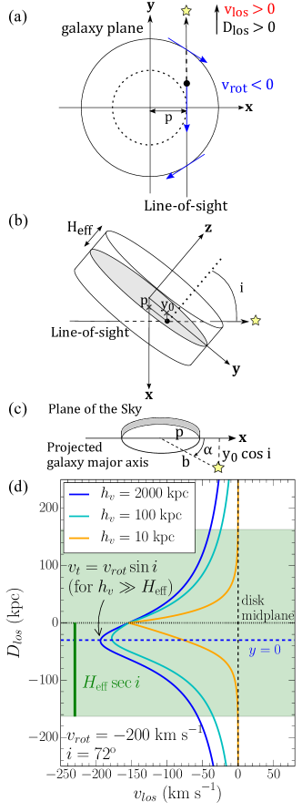
A.1. Kinematic Signatures of Circular Orbits in Disks

We adopt a right-handed coordinate system with the origin at the center of the galaxy. The $z$ -axis is perpendicular to the disk plane, i.e., the $xy$ -plane as illustrated in Figure 12. Without the loss of generality, we place the sightline in the $x=p$ plane. When projected onto the sky, the $x$ -axis is aligned with the major axis of the galactic disk, and the length of the impact parameter projected onto the galaxy major axis is $p$ . We define $y_{0}$ as the $y$ -coordinate of the sightline where it intersects the midplane of the disk. The geometry in Figure 12 shows that a sightline at azimuthal angle $\alpha$ and impact parameter $b$ is described by

p=b\cos\alpha\quad\mathrm{and}\quad y_{0}\cos i=b\sin\alpha~{}.

(A1)

This geometry allows two orientations of the disk, which are indistinguishable from galaxy morphology alone. We select the positive direction of the $z$ -axis to always lie on the quasar’s side of the disk. When the $y$ -coordinate of the quasar is positive, as shown in Figure 12, we give the inclination of the disk a positive value. To describe the situation where the disk is rotated 45^∘ about the $x$ -axis, and the $y$ -coordinate of the quasar becomes negative, we introduce the concept of a negative inclination. From the perspective of an observer, this flip about the major axis corresponds to interchanging the near and far sides of the disk. For circular orbits in the disk plane, the primary observable signature of this geometrical flip is the wrapping direction of trailing spiral arms relative to the direction of rotation.

The thickness of the disk, $H_{\mathrm{eff}}$ in Figure 12, and the vertical gradient in rotation speed can be varied to model the data. We describe the $|z|$ -dependence of the rotation speed with the exponential velocity scale height, $h_{v}$ , adopted by S02. Projection of this thick rotating disk,

\boldsymbol{v}_{\phi}(z)=v_{rot}\exp(-|z|/h_{v})\boldsymbol{\hat{\phi}}~{},

(A2)

onto the vector describing the quasar sightline,

\boldsymbol{L}=(\sin i)\boldsymbol{\hat{y}}+(\cos i)\boldsymbol{\hat{z}}~{},

(A3)

yields line-of-sight velocities

v_{los}=\boldsymbol{v}_{\phi}\cdot\boldsymbol{L}=\frac{v_{rot}\sin i}{\sqrt{1+(y/p)^{2}}}\exp\left(-\frac{|y-y_{0}|}{h_{v}\tan i}\right)~{}.

(A4)

With the right-handed coordinate system, the rotation velocity $v_{rot}$ is positive (negative) when the angular momentum vector aligns with the positive (negative) $z$ -axis of the disk. Panel (d) of Figure 12 displays $v_{los}$ along the sightline defined by

D_{los}=(y-y_{0})/\sin i~{},

(A5)

such that $D_{los}=0$ represents the midplane of the disk.

The disk thickness $H_{\mathrm{eff}}$ sets boundaries on the range of $y$ -values,

y_{0}-H_{\mathrm{eff}}\tan i<y<y_{0}+H_{\mathrm{eff}}\tan i~{},

(A6)

within the disk. The green shaded region in Figure 12(d) indicates the portion of the quasar sightline within the disk. Increasing the $H_{\mathrm{eff}}$ broadens the range of $v_{los}$ from the projected rotation speed at the point where the sightline is tangent to the disk, $v_{t}$ , toward an asymptotic value $v_{los}\rightarrow\ 0$ .

As suggested by S02, we introduce a velocity scale height $h_{v}$ to govern how quickly the rotation velocity drops from $v_{t}$ toward zero with distance along the sightline. Choosing $h_{v}>>H_{\mathrm{eff}}$ produces a linear decline in rotation speed with height above the disk

\boldsymbol{v}_{\phi}(z)\approx v_{rot}(1-|z|/h_{v})\boldsymbol{\hat{\phi}}~{}.

(A7)

As a fiducial reference point, we adopt $h_{v}=10$ kpc, which produces a vertical rotation gradient consistent with measurements for extraplanar gas above nearby galaxies (Benjamin, 2002, 2012).

The position–velocity ( $D_{los}$ vs. $v_{los}$ ) diagrams illustrate the variation in line-of-sight velocity along a particular sightline. For example, consider a very large velocity scale height, which effectively describes cylindrical rotation. In the limit $\lim h_{v}\rightarrow\infty$ , inspection of Equation (A4) shows that the maximum Doppler shift is contributed by gas at $y=0$ . The sightline is tangent to the disk at the point $y=0$ , and the maximum line-of-sight velocity becomes

v_{t}\equiv v_{los}(y=0)=v_{rot}\sin i~{}.

(A8)

The vertical velocity gradient steepens with decreasing $h_{v}$ , which moves the maximum Doppler shift along $D_{los}$ from $y=0$ toward the disk midplane. The three curves in Figure 12(d) demonstrates this shift when $h_{v}$ decreases from 2000 kpc to 10 kpc. The exponential term in Equation (A4) quantitatively describes the shift.

A.2. Kinematics Signatures of Radial Infall in the Disk Plane

We add a velocity component so that the gas motion in the disk plane becomes

\boldsymbol{v}(R,z)=\boldsymbol{v}_{R}(R,z)\boldsymbol{\hat{R}}+\boldsymbol{v}_{\phi}(R,z)\boldsymbol{\hat{\phi}}~{}.

(A9)

For purposes of illustration, we consider only constant infall speeds such that

\boldsymbol{v}_{R}(R,z)=v_{R}\boldsymbol{\hat{R}}~{},

(A10)

where $v_{R}<0$ for infalling gas.

Similar to Equation (A4), the line-of-sight velocity due to this radial velocity component alone is

v_{los,R}=\boldsymbol{v}_{R}\cdot\boldsymbol{L}=(v_{R}\sin i)\frac{y}{\sqrt{y^{2}+p^{2}}}~{},

(A11)

which gives a total line-of-sight velocity of

v_{los}=v_{los,\phi}+v_{los,R}~{}.

(A12)

The line-of-sight velocity of the radial infall changes sign along the sightline as illustrated by Figure 13. In the last column, the line-of-sight velocity from the rotation component lies entirely to one side of the systemic velocity while the infall component changes sign. The inflection point for the infall velocity corresponds to the point where the sightline is tangent to the disk, and the projected rotation component reaches a maximum.

Flipping the disk changes how the radial and azimuthal vector velocities add together. Only in the limit of large $H_{\mathrm{eff}}$ will the velocity ranges of the two orientations be identical. To our knowledge, this asymmetry has not been previously described. In the last column of Figure 13, we illustrate how the boundaries imposed by the disk thickness can lead to only one orientation producing absorption that spans the systemic velocity. We indicate the velocity range of absorption using a pair of green dashed lines. In our example, only the disk tilt with negative inclination produces absorption across the systemic velocity.

Another interesting situation is that the orientation of the flip moves the location of the maximum Doppler shift along the sightline. In our example in Figure 13, when the disk inclination is positive, the maximum Doppler shift is contributed by gas near the disk midplane. Flipping the disk, however, moves the maximum Doppler shift away from the midplane. When the model includes radial inflow, the sign of the disk inclination therefore changes the kinematics of an absorption-line system.