On the equivalence of models with similar low-energy quasiparticles

Abstract

We use a Metropolis algorithm to calculate the finite temperature spectral weight of three related models that have identical quasiparticles at $T=0$, if the exchange favors the appearance of a ferromagnetic background. The low-energy behavior of two of the models remains equivalent at finite temperature, however that of the third does not because its low-energy behavior is controlled by rare events due to thermal fluctuations, which transfer spectral weight well below the $T=0$ quasiparticle peaks and generate a pseudogap-like phenomenology. Our results demonstrate that having $T=0$ spectra with similar quasiparticles is not a sufficient condition to ensure that two models are equivalent, i.e. that their low-energy properties are similar. We also argue that the pseudogap-like phenomenology is quite generic for models of $t$-$J$ type, appearing in any dimension and for carriers injected into both ferromagnetic and antiferromagnetic backgrounds.

I Introduction

All physics knowledge is built on the study of models. Formulating a model for the system of interest is thus a key step in any project. Of course, “all models are wrong, but some of them are useful” Box and Draper . This is because ideally, a model incorporates all relevant physics of the studied system so that its solution is useful to gain intuition and knowledge regarding some properties of interest. At the same time, models discard details assumed to be irrelevant for these properties. Even though this makes them “wrong”, it is a necessary and even desirable step if the solution is to not be impossibly complicated.

How to decide where lies the separation line between relevant and irrelevant aspects for a given system and set of properties of interest, is still an art. A general guiding principle, based on perturbation theory, is that high-energy states can be discarded (integrated out) if one is interested in low-energy properties. Consequently, it is assumed that models with identical low-energy spectra provide equivalent descriptions of a system, and therefore the simplest of these models can be safely used.

A prominent example is the modeling of cuprates. It is widely believed that the Emery model Emery (1987) can be replaced by the simpler $t$-$J$ model to study their low-energy physics Lee et al. (2006); Dagotto (1994). The justification was provided by Zhang and Rice Zhang and Rice (1988) who argued that the low-energy states of the Emery model are singlets formed between the spin of a doping hole hosted on the four oxygens surrounding a copper and the spin of that copper, and that the resulting quasiparticle is described accurately by the $t$-$J$ model Anderson (1987). Whether this is true is still being debated Lau et al. (2011); Ebrahimnejad et al. (2014, ).

In this article we show that by itself, the condition that two models have the same low-energy spectrum is not sufficient to guarantee that they describe similar low-energy properties, despite widespread belief to the contrary. Indeed, we identify three models that have identical $T=0$ quasiparticles yet have very different behavior at any temperature $T\neq 0$. The qualitative differences are due to rare events controlled by thermal fluctuations, which lead to a pseudogap-type of phenomenology.

While our argument takes the form of a “proof by counterexample”, we also provide arguments that our findings are not merely an “accident” caused by our specific choice of models, but are more general in nature. Specifically, we comment on its validity in arbitrary dimensions and also for other types of magnetic coupling which differ from the examples that are our main focus.

The remainder of this article is organized as follows: we introduce the models in Section II, and discuss our method of solution in Section III. The main results, which are for a particle injected into a ferromagnetic (FM) background, are presented in Section IV.1, while Section IV.2 contains some results for an antiferromagnetic (AFM) background, which further substantiate our claims. Short conclusions are presented in Section V.

II Models

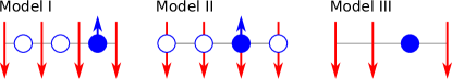
Figure 1: (color online) Sketch of the three models. Large, red arrows represent the local magnetic moments, empty (filled) blue circles represent empty (filled) carrier sites. For Models I and II the carrier spin is represented by a blue arrow, for Model III the carrier is a spinless “hole” in the Ising chain.

Because we are interested in the quasiparticle spectrum, from now on we consider only the single carrier sector of the Fock space. To be specific, we take the carrier to be an electron added into an otherwise empty band; the solution is mapped onto that for removing an electron from a full band by changing the energy $\omega\rightarrow-\omega$.

The models of interest are sketched in Fig. 1. They describe the interaction of the carrier with a background of local moments, and as such bear some similarity to those used in the Zhang-Rice mapping mentioned above. Model I is the parent two-band model, from which Models II and III are derived as increasingly simpler effective models. In Model I, one band hosts the spin$-{1\over 2}$ magnetic moments and a second band, located on a different sublattice, hosts the carrier. Model II is also a two-band model, but the carrier and local moments are located on the same sites. One can think of the states occupied by the carrier in this model as being local linear combinations of the carrier states in Model I, each centered at a spin site. In Model III, the carrier is locked into a singlet with its lattice spin, forming a “spinless carrier” analogous to the Zhang-Rice singlet.

There are also significant differences between our models and the Zhang-Rice mapping: (i) we restrict ourselves to one dimension as this suffices to prove our claim. However, some comments on the extension of our results to higher dimensions can be found below; (ii) We concentrate on the case of a ferromagnetic (FM) background because for models with an antiferromagnetic (AFM) background the $T=0$ spectra are not identical. However, we also present some AFM results later on, to demonstrate that some of the features we discuss here are generic, not FM-specific; and (iii) all spin exchanges are Ising-like, i.e. no spin flipping is allowed. The latter constraint allows us to find numerically the exact solutions using a Metropolis algorithm Möller and Berciu (2014), to uncover a surprising finite-$T$ behavior for Model III.

In all three cases, the interactions between the local moments are described by the Ising Hamiltonian:

$$\hat{H}_{S}=-J\sum_{i}\hat{\sigma}_{i+\delta}\hat{\sigma}_{i+1+\delta}-h\sum_{i}\hat{\sigma}_{i+\delta},$$ (1)

where $\delta=1/2$ for Model I and $\delta=0$ for Models II and III, and $\hat{\sigma}_{i+\delta}$ is the Ising operator for the local magnetic moment located at $R_{i+\delta}=i+\delta$ (we set $a=1$). Its eigenvalues are $\sigma_{i}=\pm 1$. For $J>0$ the ground state of $\hat{H}_{S}$ is FM, and it is AFM for $J<0$. In the case of FM coupling, the external magnetic field $h$ can be used to favor energetically one of the two possible FM ground states of the $h=0$ case.

For Models I and II, the kinetic energy of the carrier is described by a nearest-neighbor hopping Hamiltonian:

$$\hat{T}=-t\sum_{i,\sigma}c_{i,\sigma}^{\dagger}c_{i+1,\sigma}+\text{h.c.}=\sum_{k,\sigma}\epsilon(k)c_{k,\sigma}^{\dagger}c_{k,\sigma}$$ (2)

where $c_{i,\sigma}^{\dagger}$ is the creation operator for a spin-$\sigma$ carrier at site $R_{i}$ and $c_{k,\sigma}^{\dagger}=1/\sqrt{N}\sum_{i}\mathrm{e}^{ikR_{i}}c_{i,\sigma}^{\dagger}$ are states with momentum $k\in(-\pi,\pi)$ and eigenenergy $\epsilon(k)=-2t\cos k$ (the lattice constant is set to $a=1$). The interaction between the carrier and the local moments is an AFM Ising exchange:

$$\hat{H}_{\text{ex}}^{(\text{I,II})}=\frac{J_{0}}{2}\sum_{i,\sigma}\sigma c_{i,\sigma}^{\dagger}c_{i,\sigma}(\hat{\sigma}_{i-\delta}+\hat{\sigma}_{i+\delta}).$$ (3)

Note that flipping the sign of the carrier spin corresponds to letting $J_{0}\rightarrow-J_{0}$, so we can assume without loss of generality that the carrier has spin-up and suppress the spin index. The total Hamiltonian for Models I and II is thus given by $\hat{H}^{(\text{I,II})}=\hat{H}_{S}+\hat{T}+\hat{H}_{\text{ex}}^{(\text{I,II})}$.

Model III is the FM ($J>0$) or AFM ($J<0$) Ising version of the one-band $t$-$J$ model discussed extensively in the cuprate literature Lee et al. (2006); Dagotto (1994). The case of interest now has $N+1$ electrons in the $N$ site system ($N\rightarrow\infty$), and double occupancy is forbidden apart from the site where the additional carrier is located and which can be viewed as hosting a “spinless carrier” whose motion shuffles the otherwise frozen spins. The Hamiltonian is $\hat{H}^{(\text{III})}=\mathcal{P}\hat{T}\mathcal{P}+\hat{H}_{S}$, where the operator $\mathcal{P}$ projects out additional double occupancy. It is important to note that in contrast to Models I and II, here the spin-operators $\hat{\sigma}_{i}$ are related to the electron creation/annihilation operators via $\hat{\sigma}_{i}=\sum_{\sigma}\sigma c_{i,\sigma}^{\dagger}c_{i,\sigma}$.

III Method

We calculate the finite-$T$ spectral weight $A(k,\omega)=-{1\over\pi}\mbox{Im}G(k,\omega)$, where $G(k,\omega)$ is the one-carrier propagator. If the carrier is injected in the magnetic background equilibrated at temperature $T$, its real-time propagator is $G(k,\tau)=-i\theta(\tau)\mbox{Tr}[\hat{\rho}_{S}c_{k\uparrow}(\tau)c_{k\uparrow}^{\dagger}(0)]$, where $\hat{\rho}_{S}=\exp(-\beta\hat{H}_{s})/Z$ is the density matrix of the undoped chain in thermal equilibrium, $\beta=1/k_{B}T$ and $c_{k\sigma}(\tau)=\exp(i\hat{H}\tau)c_{k\sigma}\exp(-i\hat{H}\tau)$ are the operators in the Heisenberg representation (we set $\hbar=1$).

In frequency domain, the propagator becomes:

$$G(k,\omega)=\sum_{\{\sigma\}}\frac{\mathrm{e}^{-\beta E^{S}_{\{\sigma\}}}}{Z}\langle\{\sigma\}|c_{k\uparrow}\hat{G}(\omega+E^{S}_{\{\sigma\}})c_{k\uparrow}^{\dagger}|\{\sigma\}\rangle$$

The sum is over all configurations $\{\sigma\}=(\sigma_{1},\dots,\sigma_{N})$ of the Ising chain, with corresponding energies $\hat{H}_{S}|\{\sigma\}\rangle=E^{S}_{\{\sigma\}}|\{\sigma\}\rangle$, and $Z=\sum_{\{\sigma\}}\exp(-\beta E^{S}_{\{\sigma\}})$. The resolvent is $\hat{G}(\omega)=[\omega-\hat{H}+i\eta]^{-1}$, where $\eta\rightarrow 0^{+}$ ensures retardation. The shift by $E^{S}_{\{\sigma\}}$ in the argument of the resolvent shows that the poles of the propagator mark the change in the system’s energy, i.e. the difference between the eigenenergies of the system with the carrier present, and those of the undoped states into which it was injected. This reflects the well-known fact that electron addition states have poles at energies $E_{N+1,\alpha}-E_{N,\beta}$ Mahan (2000).

After Fourier transforming to real space and using the invariance to translations of the thermally averaged system, we arrive at:

$$G(k,\omega)=\sum_{n}\mathrm{e}^{ikR_{n}}\sum_{\{\sigma\}}\frac{\mathrm{e}^{-\beta E^{S}_{\{\sigma\}}}}{Z}g_{0,n}(\omega,\{\sigma\}),$$ (4)

where $g_{0,n}(\omega,\{\sigma\})=\langle\{\sigma\}|c_{0,\uparrow}\hat{G}(\omega+E^{S}_{\{\sigma\}})c_{n,\uparrow}^{\dagger}|\{\sigma\}\rangle$ is the Fourier transform of the amplitude of probability that a state with configuration $\{\sigma\}$ and the carrier injected at site $n$ evolves into a state with the carrier injected at site $0$. These real-space propagators are straightforward to calculate, as they correspond to a single particle (consistent with our assumption of a canonical ensemble with exactly one extra charge carrier in the system) moving in a frozen spin background. We emphasize that this is true only because of the Ising nature of the exchange between the background spins. Heisenberg coupling, on the other hand, would lead to spin fluctuations that would significantly complicate matters. Below we present the calculation of these real-space propagators for Model III. For Model II, the solution is described in detail in Ref. Möller and Berciu, 2014, and the same approach, with only minor modifications, applies to Model I.

It is convenient to introduce the following notation. When an extra electron is injected at site $n$ of Model III it effectively removes the spin at this site. The spin $\sigma_{n}$ will therefore be missing from the set $\{\sigma\}$ which describes the state of the spin-chain before injection. Consequently we label the new state, after injection, as $|\{\sigma\}\setminus\sigma_{n}\rangle=|\dots\sigma_{n-1}\circ\sigma_{n+1}\dots\rangle$, where $\circ$ denotes the effective “hole” created by the injection of the extra electron. The “hole” can propagate along the chain and in doing so reshuffles the spins. To capture the propagation of the “hole” we introduce a new index $j$ corresponding to the number of sites that the “hole” has hopped to the left ($j<0$) or right ($j>0$). A general state is therefore given by $|\{\sigma\}\setminus\sigma_{n},j\rangle=|\dots\sigma_{n-1}\sigma_{n+1}\dots\sigma_{n+j}\circ\sigma_{n+j+1}\rangle$. Note that this way of labelling states is not unique. For instance, if $\sigma_{0}=\sigma_{1}=\dots=\sigma_{n}$, then $|\{\sigma\}\setminus\sigma_{0},0\rangle=|\{\sigma\}\setminus\sigma_{n},-n\rangle$.

With this notation, the real-space propagators are $g_{0,n}(\omega,\{\sigma\})=\langle\{\sigma\}\setminus\sigma_{0},0|\hat{G}(\omega+E^{S}_{\{\sigma\}})|\{\sigma\}\setminus\sigma_{n},0\rangle$. Their equations of motion (eom) are obtained by splitting the Hamiltonian in two parts, $\hat{H}=\hat{H}_{0}+\hat{V}$, and repeatedly using Dyson’s identity $\hat{G}(\omega)=\hat{G}_{0}(\omega)+\hat{G}(\omega)\hat{V}\hat{G}_{0}(\omega)$. Choosing $\hat{H}_{0}=\hat{H}_{S}$ and suppressing the $\omega$ and $\{\sigma\}$-dependence we obtain

$$g_{0,0} =G_{0}(\omega+\Delta_{0})[1-tf_{0,1}-tf_{0,-1}],$$ (5)

$$f_{0,n} =-tG_{0}(\omega+\Delta_{n})[f_{0,n+1}+f_{0,n-1}],$$ (6)

where $G_{0}(\omega)=(\omega+i\eta)^{-1}$, $\Delta_{n}=E^{S}_{\{\sigma\}}-E^{S}_{\{\sigma\}\setminus\sigma_{0},n}$ and $f_{0,n}=\langle\{\sigma\}\setminus\sigma_{0},0|\hat{G}(\omega+E^{S}_{\{\sigma\}})|\{\sigma\}\setminus\sigma_{0},n\rangle$. Note that $f_{0,0}=g_{0,0}$. The exact form of $\Delta_{n}$ depends on the sign of $n$:

$$\Delta_{0} =-J\sigma_{0}(\sigma_{-1}+\sigma_{1})$$ (7)

$$\Delta_{n} =\Delta_{0}+J\sigma_{-1}\sigma_{1}-J\sigma_{n}\sigma_{n+1},\ \text{for}\ n>0$$ (8)

$$\Delta_{n} =\Delta_{0}+J\sigma_{-1}\sigma_{1}-J\sigma_{n}\sigma_{n-1},\ \text{for}\ n<0.$$ (9)

The eom (6) can be solved with the ansatz $f_{0,n}=A_{n}f_{0,n-1}$, for $n>0$ and $f_{0,n}=B_{n}f_{0,n+1}$ for $n<0$. Since the “hole” has a finite lifetime $\propto 1/\eta$ and $f_{0,n}$ measures the probability that the “hole” injected at site 0 moves to site $n$, one expects $f_{0,n}\rightarrow 0$ for $n\rightarrow\infty$. We therefore introduce a sufficiently large cutoff $M_{c}$ and require $A_{M_{c}}=0=B_{-M_{c}}$. It is then straightforward to obtain

$$A_{n} =\frac{-t}{\omega+\Delta_{n}+i\eta+tA_{n+1}},$$ (10)

$$B_{n} =\frac{-t}{\omega+\Delta_{n}+i\eta+tB_{n-1}},$$ (11)

$$g_{0,0} =\frac{1}{\omega+\Delta_{0}+tB_{-1}+tA_{1}},$$ (12)

$$f_{0,n} =A_{n}\dots A_{1}g_{0,0} \text{for}\ n>0,$$ (13)

$$f_{0,n} =B_{n}\dots B_{1}g_{0,0} \text{for}\ n<0.$$ (14)

To calculate the $g_{0,n}$ we make use of the fact that hopping reshuffles the spins. Therefore $g_{0,n}\neq 0$, only if $\sigma_{0}=\sigma_{1}=\dots=\sigma_{n}$. In that case, as mentioned above, the states $|\{\sigma\}\setminus\sigma_{0},n\rangle$ and $|\{\sigma\}\setminus\sigma_{n},0\rangle$ are equal which means that $g_{0,n}=f_{0,n}$.

The thermal average in Eq. (4) is then calculated for the infinite chain with a Metropolis algorithm which generates configurations $\{\sigma\}$ of the undoped chain. To summarize, our method of solution consists of the following steps: (i) generate a configuration $\{\sigma\}$ of the Ising chain using a Metropolis algorithm; (ii) Calculate all the $g_{0,n}(\omega,\{\sigma\})$ propagators for that specific configuration, and perform the sum over $n$ in Eq. (4); (iii) repeat steps (i) and (ii) until convergence is reached. Full details of this procedure can be found in Ref. Möller and Berciu, 2014 for Model II; the generalization to Models I and III is straightforward. For Model III it is convenient to inject the carrier with an unpolarized total spin, to ensure that a “hole” is always created. Since for each configuration $\{\sigma\}$ there is a configuration $\{\bar{\sigma}\}$ with all the spins flipped, injecting an unpolarized carrier does not change the results, but merely speeds up the numerics.

IV Results

IV.1 FM Results

At $T=0$, the undoped Ising chain is in its FM ground state. The quasiparticles of Models I and II have energy $\mp J_{0}+\epsilon(k)$ if the carrier is injected with its spin antiparallel/parallel to the background. Only the former case can be meaningfully compared with Model III, which has a quasiparticle of energy $2J+\epsilon(k)$ ($2J$ is the cost of removing two FM Ising bonds). Thus, apart from trivial shifts, the three models have identical quasiparticles, namely carriers free to move in the otherwise FM background.

Finite-$T$ spectral weights $A(k=0,\omega)$ for the different models are shown in Fig. 2. We emphasize that only the electron-addition part is discussed here. We do not consider the electron-removal states, which lie at energies well below those of the electron-addition states and must be identical for all three models because in all cases, one of the electrons giving rise to the magnetic moments is removed. We also emphasize that our calculation is in a canonical ensemble. The chemical potential is not fixed at $\omega=0$, as customary in grand canonical formulations, instead it can be calculated as $\mu=\left({\partial F\over\partial N}\right)_{T}\rightarrow\min_{\alpha,\beta}[E_{N+1,\alpha}-E_{N,\beta}]$ as $T\rightarrow 0$. As pointed out above, here $\omega=0$ marks the energy of the undoped Ising chain.

For Models I and II, shown in panels (a) and (b), at the lowest temperature one can see two peaks marking the contributions from injection of the carrier into the two ground states of the Ising chain (all spins up and all spins down, respectively). Indeed, these peaks are located at $\pm J_{0}-2t$, the lower one of which is marked by the vertical line. Note that we chose a large $J_{0}$ value to keep different features well separated and thus easier to identify. The insets show the spectral weights for $h=-0.1t$, which at low-$T$ suppresses the contribution from the up-spin FM state so that only the lower peak remains visible.

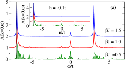
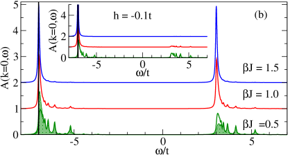
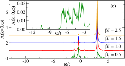
Figure 2: (color online) Spectral weight at $k=0$ for a FM background and three different temperatures for (a) Model I with $J_{0}/t=5,J/t=0.5$; (b) Model II with $J_{0}/t=5,J/t=0.5$; (c) Model III with $J/t=2.5$. Insets in panels (a) and (b) show the spectral weight in the presence of a magnetic field, while in (c) it shows the two continua appearing at low energies, for $\beta J=0.5$. In all cases, the broadening is $\eta/t=0.04$. The vertical lines show the energy of the $T=0$ quasiparticle peak.

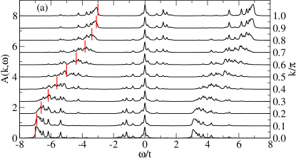
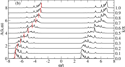
Figure 3: (color online) $A(k,\omega)$ for the three models with FM background at $\beta J=0.5$. Other parameters are as in Fig. 2. The dispersionless low energy, low weight part of the spectrum of Model III is not shown. Red, vertical lines indicate the location of the $T=0$ quasiparticle peaks.

With increasing $T$, both peaks broaden considerably on their higher-energy side, and many resonances become visible. As demonstrated in Ref. Möller and Berciu, 2014 for Model II, these resonances are due to temporal trapping of the carrier inside small magnetic domains that are thermally generated at higher $T$. The presence of these domains also explains the decreasing difference between the $h=0$ and $h=-0.1t$ curves at higher $T$. For $\beta J=0.5$ both curves are shown in the main panels (the finite $h$ curve is shaded in). Indeed, the resonances appear in the same places and with equal weight in both curves, the only difference being a small spectral weight transfer from $J_{0}-2t$ to $-J_{0}-2t$, i.e. from the FM ground-state disfavored by $h<0$ to the one favored by it. The weight for the former is no longer zero like for $T\rightarrow 0$, showing that at higher-$T$ the carrier is increasingly more likely to explore longer domains of spin-up local moments.

The main difference between Models I and II is that the latter also has a third finite-$T$ continuum, centered around $\omega=0$. It corresponds to injecting the carrier in small AFM domains, where its exchange energy vanishes because it sits between a spin-up and a spin-down local moment. Such energy differences are not possible in Model II, where the carrier interacts with a single moment so its exchange energy is $\pm J_{0}$.

However, if one is interested in the low-energy behavior, Models I and II are equivalent because their low-energy continua have similar origins and evolve similarly with $T$. This is true in the whole Brillouin zone (BZ), as can be seen from comparing panels (a) and (b) of Fig. 3.

The finite-$T$ evolution of the spectral weight of Model III is very different. Consider first the $k=0$ case, shown in Fig. 2(c). The $T=0$ peak at $2J-2t$ (marked by the vertical line) evolves with $T$ very similarly to the low-energy peaks of the other two models, broadening on its high-energy side and again displaying resonances due to temporal trapping inside small domains. The $k$ evolution of this feature, shown in Fig. 3(c), is also very similar to the low-energy continua of the other two models.

However, for Model III this continuum is not the low-energy feature. Instead, in 1d there are three lower-energy continua centered at $0,-2J$ and $-4J$, all of which are due to injection of the carrier into specific, thermally excited configurations of the background. For example, consider the $-2dJ$ continuum which also appears in dimensions $d>1$. As sketched in Fig. 4, it corresponds to the carrier being paired with a thermally excited spin. This lowers the exchange energy by $2dJ$, as $2d$ AFM bonds are broken. In contrast, $T=0$ doping always leads to loss of exchange energy, because only FM bonds can be broken. This is why in Model III it can cost less energy to dope from a thermally excited state rather than the ground-state, and therefore why its finite-$T$ low-energy properties are not controlled by the $T=0$ quasiparticle.

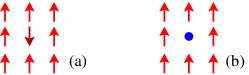
Figure 4: (color online) When doping “removes” a thermally excited spin-down, the energy variation upon doping is $E_{b}-E_{a}=-2dJ+\epsilon(k)$ and lies (at least partially) below the $T=0$ quasiparticle ground-state energy of $2dJ-2dt$.

The weight of these low-energy continua is very small, see inset of Fig. 2(c), because they are controlled by thermal activation. For example, in the limit $T\rightarrow 0$ the spectral weight of the continuum centered at $-2dJ$ can be calculated to first order, as was shown in Refs Möller and Berciu, 2013, 2014, by expanding Eq. (4) in powers of $\mathrm{e}^{-\beta 4dJ}$. The lowest order terms correspond to the two FM ground states which have all spins aligned, $|\{\uparrow\}\rangle$ and $|\{\downarrow\}\rangle$, respectively. The first order terms are given by states with a single flipped spin and are denoted by $|\{\uparrow,\sigma_{m}=\downarrow\}\rangle$ and $|\{\downarrow,\sigma_{m}=\uparrow\}\rangle$, where $m$ indicates the location of the flipped spin. Since the flipped spin can be anywhere in the system there are $N$ of these states for each ground state configuration. For simplicity we assume that the spin of the extra carrier is unpolarized, then it suffices to consider only $|\{\uparrow\}\rangle$ and $|\{\uparrow,\sigma_{m}=\downarrow\}\rangle$, the contribution from the other ground state will be exactly the same. Considering only these states in the trace of Eq. (4) we obtain:

$$G(\mathbf{k},\omega)= \frac{1}{Z^{\prime}}[\mathcal{G}^{(0)}(\mathbf{k},\omega)+\mathrm{e}^{-\beta 4dJ}\mathcal{G}^{(1)}(\mathbf{k},\omega)]$$

$$+\mathcal{O}((\mathrm{e}^{-\beta 4dJ})^{2}),$$ (15)

where

$$\mathcal{G}^{(0)}(\mathbf{k},\omega)= [\omega-\epsilon_{\mathbf{k}}-2dJ+i\eta]^{-1}$$ (16)

$$\mathcal{G}^{(1)}(\mathbf{k},\omega)= \sum_{n,\sigma}\mathrm{e}^{i\mathbf{k}\mathbf{R}_{n}}\sum_{m}g_{0,n}(\omega,\{\uparrow,\sigma_{m}=\downarrow\})$$ (17)

$$Z^{\prime}= \frac{Z}{\mathrm{e}^{-\beta E_{\text{FM}}}}=(1+N\mathrm{e}^{-\beta 4dJ}+\dots)$$ (18)

Note that $\mathcal{G}^{(0)}(\mathbf{k},\omega)$ is identical to the $T=0$ solution.

To evaluate $\mathcal{G}^{(1)}(\mathbf{k},\omega)$ we need to treat the case $m=0$, separately. In this case the extra carrier removes the flipped spin. This results in the breaking of $2d$ AFM bonds and therefore an energy gain of $2dJ$. Furthermore as pointed out above only $g_{0,0}(\omega,\{\uparrow,\sigma_{0}=\downarrow\})$ contributes to the sum since the extra carrier was injected into a domain of length 1. Since the flipped spin was removed and all the remaining spins are aligned it is easy o calculate $g_{0,0}(\omega,\{\uparrow,\sigma_{0}=\downarrow\})$ which in the limit $N\rightarrow\infty$ becomes

$$g_{0,0}(\omega,\{\uparrow,\sigma_{0}=\downarrow\})=\int\frac{d\mathbf{q}}{(2\pi)^{d}}\frac{1}{\omega-\epsilon_{\mathbf{q}}+2dJ+i\eta},$$ (19)

i.e. a continuum of states centered at $\omega=-2dJ$.

We are now left with calculating the remaining contributions to $\mathcal{G}^{(1)}(\mathbf{k},\omega)$ for which $m\neq 0$. This is not a trivial problem, but since there is only one flipped spin in the system and we are summing over all “hole” locations, we can approximate $g_{0,n}(\omega,\{\uparrow,\sigma_{m}=\downarrow\})\approx g_{0,n}(\omega,\{\uparrow\})$. In doing so we neglect that the energy is lowered when the “hole” is adjacent to the flipped spin $\sigma_{m}$. Reinserting into Eq. (17) we obtain

$$\mathcal{G}^{(1)}(\mathbf{k},\omega)\approx g_{0,0}(\omega,\{\uparrow,\sigma_{0}=\downarrow\})+(N-1)\mathcal{G}^{(0)}(\mathbf{k},\omega),$$ (20)

where the factor $N-1$ in front of $\mathcal{G}^{(0)}$ is due to the sum over $m$. Note that this factor ensures that the $Z^{\prime}$ in the Eq. for $G(\mathbf{k},\omega)$ is approximately canceled. Similarly one expects contributions from states with two or more well-separated flipped spins to cancel the $Z^{\prime}$ in front of $g_{0,0}(\omega,\{\uparrow,\sigma_{0}=\downarrow\})$ Möller and Berciu (2013, 2014). Consequently the low-$T$ expansion of the Green’s function gives:

$$G(\mathbf{k},\omega)\approx\mathcal{G}^{(0)}(\mathbf{k},\omega)+\mathrm{e}^{-\beta 4dJ}g_{0,0}(\omega,\{\uparrow,\sigma_{0}=\downarrow\}).$$ (21)

i.e. the spectral weight below the $T=0$ quasiparticle which is given by $g_{0,0}(\omega,\{\uparrow,\sigma_{0}=\downarrow\})$ vanishes like the probability $\mathrm{e}^{-\beta 4dJ}$ to find a flipped spin.

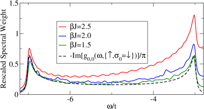
Figure 5: (color online) Rescaled spectral weight $\mathrm{e}^{\beta 4J}[A(0,\omega)-A^{(0)}(0,\omega)]$ in the region of the continuum centred at $-2J$, for Model III with FM background and different values of $\beta$. For comparison the dashed, black line shows $-\text{Im}[g_{0,0}(\omega,\{\uparrow,\sigma_{0}=\downarrow\})]/\pi$ calculated with Eq. (19). Other parameters are $J/t=2.5$ and $\eta/t=0.04$.

To verify this behavior we show in Fig. 5 the rescaled spectral weight $\mathrm{e}^{\beta 4J}[A(0,\omega)-A^{(0)}(0,\omega)]$, where $A^{(0)}(k,\omega)=\delta(\omega-\epsilon_{k}-2J)/\pi$ is the $T=0$ quasiparticle peak. From Eq. (21) it is clear that at sufficiently low $T$ the resulting curves should equal $-\text{Im}[g_{0,0}(\omega,\{\uparrow,\sigma_{0}=\downarrow\})]/\pi$, which is shown by the dashed, black line in Fig. 5. Indeed we find that the three curves in Fig. 5 for $\beta J=1.5$, $2.0$ and $2.5$, respectively, collapse onto each other and onto the curve for $-\text{Im}[g_{0,0}(\omega,\{\uparrow,\sigma_{0}=\downarrow\})]/\pi$. Close to the upper edge of the continuum the agreement starts to falter. This is because in addition to the $T=0$ peak there are other peaks in the spectral weight (see Fig. 2) whose tails contribute to the $-2J$ continuum and are not subtracted. Multiplying with $\mathrm{e}^{\beta 4J}$ amplifies these tails. Similarly the oscillating features in Fig. 5 are numerical artefacts which are amplified by the factor $\mathrm{e}^{\beta 4J}$.

Similar calculations can be performed for the other low-energy features. All their spectral weights vanish as $T\rightarrow 0$ because they all originate from doping the carrier into a thermally excited environment, which become less and less likely to occur in this limit.

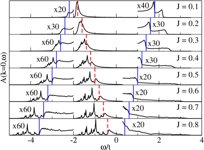
Figure 6: (color online) $A(k=0,\omega)$ for Model III with FM background, for different values of $J$ at a temperature $\beta J=0.5$. The dashed red lines show the location of the $T=0$ quasiparticle peak. Full blue lines mark the energies $-2J\pm 2t$. Parts of the spectra have been rescaled for better visibility.

The finite-$T$ behavior of Model III is thus qualitatively different from that of Models I and II. For the latter, the $T=0$ quasiparticle peak also marks the lowest energy for electron-addition at any finite temperature, whereas for Model III we observe the appearance of electron-addition states well below the $T=0$ quasiparticle peak. Their spectral weight vanishes as $T\rightarrow 0$, which is very reminiscent of pseudogap behavior and offers a simple and general scenario for how it can be generated. These low-energy states vanish from the spectrum as the temperature is lowered not because a gap opens and/or the electronic properties are somehow changed, but simply because these states describe doping into thermally excited local configurations, and the probability for the doped carrier to encounter them vanishes as $T\rightarrow 0$.

As should be clear from these arguments, the appearance of these low-energy continua is not a consequence of the large $J/t$ values used so far for Model III. Indeed, Fig. 6 shows that similar behavior is observed for smaller $J$ values (parts of these spectral weights have been rescaled for better visibility). With decreasing $J$ the different continua overlap, but shoulders marking some of their edges are still clearly visible and marked by dashed lines. In all cases, at finite $T$ spectral weight appears below the $T=0$ quasiparticle peak, marked by the full line.

It should also be clear that this phenomenology is not restricted to FM backgrounds, either: one can easily think of excited configurations in an AFM background whose exchange energy would be lowered through doping, in a $t$-$J$ model similar to Model III. We have verified numerically that at finite-$T$, features lying below the corresponding $T=0$ quasiparticle peak indeed appear in the spectral weight of AFM chains. These results are presented below. This phenomenology is therefore quite general.

IV.2 AFM Results

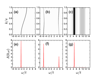
Figure 7: (color online) $T=0$, AFM solutions. Top panels: contour plots of $A(k,\omega)$. Bottom panels: Cross sections at $k=0$. (a) and (d) Model I with $J_{0}/t=5$, $|J|/t=0.5$; (b) and (e) Model II with $J_{0}/t=5$, $|J|/t=0.5$; (c) and (f) Model III with $|J|/t=2.5$. To improve visibility of the continuum a hard cutoff at $A(k,\omega)=0.1$ was used for the Model III contour plot. In all cases $\eta/t=0.04$.

Just like in the FM case, there are also two ground states of the undoped AFM Ising chain: either the odd or the even lattice hosts the up spins. Of course, both AFM ground states yield the same quasiparticle properties. However, the quasiparticles that result when a carrier is injected in the three models are different even at $T=0$, for the AFM backgrounds. This is shown in Fig. 7, where contour plots of the $T=0$ spectral weight $A(k,\omega)$, and cross sections at $k=0$, are shown.

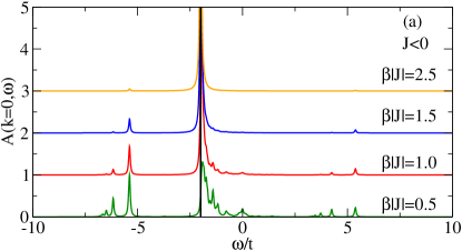
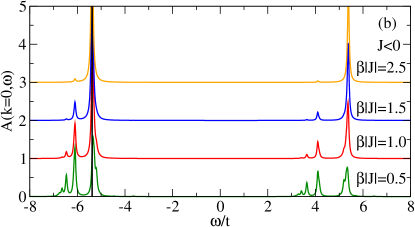
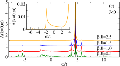
Figure 8: (color online) AFM Spectral weight at $k=0$ for three different temperatures for (a) Model I with $J_{0}/t=5,|J|/t=0.5$; (b) Model II with $J_{0}/t=5,|J|/t=0.5$; (c) Model III with $|J|/t=2.5$, the inset shows spectral weight below the $T=0$ quasiparticle peak for $\beta|J|=2.5$. In all cases,the broadening is $\eta/t=0.04$. The vertical lines show the energy of the $T=0$ quasiparticle peak.

For Model I, the energy shifts due to the Ising exchange with the spins to the left and right of the extra electron exactly cancel out and the quasiparticle behaves like a free electron with dispersion $\epsilon(k)$. For Model II, interaction with the AFM background opens a gap in the quasiparticle spectrum and halves its BZ. The upper and lower bands have dispersion $\pm\sqrt{J_{0}^{2}+\epsilon^{2}(k)}$, respectively. For Model III, the $T=0$ spectral function is independent of $k$ and has a coherent quasiparticle peak at $\omega=4|J|-2\sqrt{J^{2}+t^{2}}$ and a continuum for $4|J|-2t<\omega<4|J|+2t$. The quasiparticle peak corresponds to a bound state with the extra electron confined at its injection site. Propagation of the extra electron along the chain reshuffles the Ising spins and gives rise to the continuum centered at $4|J|$. One can therefore think of this continuum as the electron+magnon continuum. Mathematically, the $k$-independence follows directly from the fact that for Model III, $g_{0,n}(\omega,\{\sigma\})=0$ when $n>0$, if $\{\sigma\}$ is the AFM ground state.

The finite-$T$ spectral functions for $k=0$ are shown in Fig. 8. For all three models the peaks broaden and spectral weight appears below, as well as above the $T=0$ quasiparticle peak. This is in contrast to the FM case, where in Models I and II, at $k=0$, spectral weight appears only above the $T=0$ quasiparticle peak. For Model I the energy difference between the low-energy states and the $T=0$ peak is controlled by $J_{0}$, whereas for Model II it is of the order of $t$. Just as for the FM case, these features can be linked to small domains which temporarily trap the carrier Möller and Berciu (2014). As the temperature increases more weight is transferred to these low-energy features, and the low-energy behavior of Model II starts to resemble that of Model I even though they have different $T=0$ quasiparticles.

For Model III, at finite-$T$ new features appear, centered at $-2|J|$ and $0$. Just as for the FM case, they are due to the injection of the extra electron into specific, excited, local configurations of the chain. If the electron is injected into a small FM domain embedded in an otherwise AFM ordered background, the energy is lowered by $2d|J|$. As long as the electron stays within the FM domain reshuffling of the spins does not result in a further change in energy. This explains the appearance of spectral weight at $\omega\sim-2d|J|$. This is true for any dimension $d$ and consequently the appearance of spectral weight at $-2d|J|$ is a generic feature of Model III. Coming back to the specific case of $d=1$, if the electron leaves the FM domain reshuffling of the spins recreates an FM bond and destroys one of the AFM bonds. The total change in energy (injection and reshuffling) is therefore zero, explaining the continuum centered around $\omega\sim 0$. Besides the appearance of these new, low-energy continua, resonances appear close to the $T=0$ quasiparticle peak and within the high-energy continuum (not visible in Fig. 8 due to the scale). They are likely caused by injection of the electron into an AFM domain and subsequent scattering off domain walls which can only exist at finite-$T$.

V Conclusions

In this work, we identified models that have identical $T=0$ low-energy quasiparticles (for couplings favoring a FM background), and yet exhibit very different low-energy behavior at finite $T$, proving that the former condition does not automatically guarantee the latter.

In particular, the finite-$T$ behavior in Model III is controlled by rare events, where the carrier is injected into certain magnetic configurations created by thermal fluctuations. Their energies are higher than that of the undoped ground-state, however the spectral weight measures the change in energy upon carrier addition (or removal), and this may be lower at finite-$T$ than at $T=0$. This is the case for Model III because here doping removes a magnetic moment from the background while its motion reshuffles the other ones. It is not the case for Models I and II where the carrier can do neither of these things. This difference is irrelevant at $T=0$ because of the simple nature of the undoped FM ground-state, but becomes relevant at finite-$T$.

We showed that such transfer of finite-$T$ spectral weight well below the $T=0$ quasiparticle peak is independent of the size of the magnetic coupling $J$ and occurs for both FM and AFM coupling. Furthermore, we provided arguments that this behavior is expected to occur in any dimension.

While far from being a comprehensive study, these results clearly demonstrate that the appearance of finite-$T$ spectral weight well below the quasiparticle peak, due to the injection of the carrier into a thermally excited local environment making it behave very unlike the $T=0$ quasiparticle, is a rather generic feature for $t$-$J$ like models. The weight of these finite-$T$, low-energy features must vanish when $T\rightarrow 0$ because the probability for such excited environments to occur vanishes, therefore these models exhibit generic pseudogap behavior.

- (1) G. E. P. Box and N. R. Draper, Empirical Model-Building and Response Surfaces (Wiley, 1987).
- Emery (1987) V. J. Emery, Phys. Rev. Lett. 58, 2794 (1987).
- Lee et al. (2006) P. A. Lee, N. Nagaosa, and X.-G. Wen, Rev. Mod. Phys. 78, 17 (2006).
- Dagotto (1994) E. Dagotto, Rev. Mod. Phys. 66, 763 (1994).
- Zhang and Rice (1988) F. C. Zhang and T. M. Rice, Phys. Rev. B 37, 3759 (1988).
- Anderson (1987) P. W. Anderson, Science 235, 1196 (1987).
- Lau et al. (2011) B. Lau, M. Berciu, and G. A. Sawatzky, Phys. Rev. Lett. 106, 036401 (2011).
- Ebrahimnejad et al. (2014) H. Ebrahimnejad, G. A. Sawatzky, and M. Berciu, Nature Phys. 10, 951 (2014).
- (9) H. Ebrahimnejad, G. A. Sawatzky, and M. Berciu, arXiv:1505.04405 .
- Möller and Berciu (2014) M. Möller and M. Berciu, Phys. Rev. B 90, 075145 (2014).
- Mahan (2000) G. D. Mahan, Many-Particle Physics (Springer, 2000).
- Möller and Berciu (2013) M. Möller and M. Berciu, Phys. Rev. B 88, 195111 (2013).