Primordial gravitational waves in supersolid inflation

Abstract

Supersolid inflation is a class of inflationary theories that simultaneously breaks time and space reparameterization invariance during inflation, with distinctive features for the dynamics of cosmological fluctuations. We investigate concrete realizations of such a scenario, including non-minimal couplings between gravity and the fields driving inflation. We focus in particular on the dynamics of primordial gravitational waves and discuss how their properties depend on the pattern of symmetry breaking that we consider. Tensor modes can have a blue spectrum, and for the first time we build models in which the squeezed limit of primordial tensor bispectra can be parametrically enhanced with respect to standard single-field scenarios. At leading order in a perturbative expansion, the tensor-to-scalar ratio depends only on the parameter controlling the breaking of space-reparameterization. It is independent from the quantities controlling the breaking of time-reparameterization, and this represents a difference with respect to standard single-field inflationary models.

1 Introduction

The simplest approach to inflation couples gravity with a single scalar field with a flat potential. The scalar field dynamics varies from model to model, but a common feature of all single-field inflationary models is the breaking of time-reparameterization of de Sitter space during inflation. This suggests that predictions of different inflationary scenarios can be understood in terms of the language of effective field theory applied to cosmology. Indeed, in appropriate regimes, the curvature perturbation ${\cal R}$ can be related with the Goldstone boson of the broken time-reparameterization of de Sitter space. This is the spirit of the effective field theory of inflation (EFTI), started with the work [1] (see also [2], and e.g. [3] for a review).

One of the most interesting lessons of the EFTI is a new perspective to inflation, that can be seen as a symmetry breaking process. Such viewpoint naturally motivates the exploration of more general symmetry breaking patterns, besides the minimal one which breaks time-reparameterization only. For example, one can consider models which break also space-reparameterization during inflation. This is a possibility studied in systems with vector fields [4] or in models with scalars as solid inflation [5, 6]. Vector models of inflation are delicate since, in the minimal set-ups, the longitudinal vector polarization becomes a ghost around accelerating spacetimes [7]. This can be cured in scenarios as gauge or chromo-natural inflation [8, 9, 10], or in models where vectors are spectator fields: see e.g. the review [11]. The study of cosmological perturbations in vector models leads to interesting features, as possible breaking of isotropy in the scalar power spectrum, or a direction dependent squeezed limit of the scalar bispectrum: see e.g. [12]. Also models with scalar fields can lead to similar features. In solid inflation [5], a set of three scalar fields interact derivatively, and spontaneously breaks space-reparameterization during inflation. The scalar curvature perturbation is characterized by a single dynamical non-adiabatic mode, which can be thought as corresponding to a phonon propagating in the ‘solid’ inflationary medium. Such set-up has several distinctive observational features: among others, a blue spectrum for tensor modes, and a direction dependent squeezed limit for the scalar three-point function (with different angular dependence with respect to the aforementioned vector models).

In this work, inspired by an EFTI perspective, we consider a scenario of supersolid inflation, in which a set of four scalar fields breaks both time and space reparameterizations during inflation (and the name supersolid is borrowed from condensed matter nomenclature [13]). A similar scenario has already been considered in [14], showing that the dynamics of curvature perturbations has interesting features: the scalar three-point function has a more general direction-dependent squeezed limit, which interpolates between the results of vector and solid inflation, a blue spectrum for tensor modes potentially detectable by future interferometers, like the Laser Interferometer Space Antenna (LISA) [15] and an enhanced three-point function for graviton-scalar-scalar fluctuations.

We reconsider the scenario of supersolid inflation adding some key ingredients, as a non-minimal coupling between the scalar fields and the curvature, with the specific aim to point out new features with respect to the primordial tensor power spectrum. We build concrete models where the dynamics of cosmological perturbations is straightforward to handle, and lead to interesting consequences for the properties of the tensor spectrum, which make them distinguishable from single-field scenarios of inflation. The main distinctive results are a parametrically enhanced tensor non-Gaussianity peaked in a squeezed configuration, and the identification of an interesting corner in parameter space where the tensor-to-scalar ratio is only controlled by the parameters which break space translation during inflation (and not by the slow-roll parameter $\epsilon_{H}\,=\,-\dot{H}/H^{2}$, which controls the breaking of time-reparametrization). For simplicity, we do not study here the most general action compatible with our requirements, but we focus on the simplest scenarios with the properties we intend to investigate.

We summarize our results in the following bullet points:

• We start with Section 2, presenting the scalar-tensor action we build, with a new non-minimal couplings between the scalars and curvature. Inflationary models of supersolid inflation are conveniently described in terms of three dimensionless parameters, which control respectively the breaking of time-reparameterization, space-reparameterization and de Sitter invariance during inflation. We present two explicit models of inflation, one corresponding to a system in pure de Sitter space, the other to a model of power law inflation.

• In Section 3 we investigate the dynamics of tensor modes. For the first time in scenarios breaking space-reparameterization, we calculate the tensor action up to third order in perturbations. At second order in a perturbative expansion in the fluctuations, we find that tensors have both a mass different from zero, and a sound speed different than one. We compute the tensor power spectrum, confirming that tensor fluctuations can have a blue spectrum when the underlying geometry deviates from de Sitter [5]. At third order, the tensor action acquires contributions that are different from the ones characterising single-field inflationary models. We compute the corresponding contributions to tensor non-Gaussianity, finding a possible parametric enhancement of tensor bispectra in their squeezed limit with respect to single-field scenarios.

• Section 4 discusses the dynamics of scalar fluctuations. In a set-up as supersolid inflation, we expect two dynamical scalar modes: one associated with the breaking of time translations, the other with the breaking of space-reparameterizations. In the concrete models we analyse, the couplings among these two scalars can lead to an intricate coupled dynamics. Interestingly, we identify a corner in parameter space where the analysis simplifies considerably: we consider an expansion at leading and next to leading order in the parameter breaking time-reparameterization – while we keep an arbitrary size for the parameter breaking space-reparameterization. At leading (zeroth) order in this expansion, we find that only one scalar mode propagates, related to the comoving curvature fluctuation ${\cal R}$, and the amplitude of its power spectrum is independent from quantities controlling the breaking of time-reparameterization. As an interesting consequence, in these scenarios the tensor-to-scalar ratio only depends on the parameter breaking space-reparameterization contrarily to what usually happens in standard models of inflation driven by a single field. We discuss some ramifications of this feature for the effective field theory of inflation and the Lyth bound.

We conclude in Section 5 where we summarize our results and discuss possible future developments. Appendix A contains some useful technical details.

2 System under consideration

We consider a system of four scalar fields: $\phi$ and $\sigma^{I}$, $I\,=\,1,2,3$ whose vacuum expectation values (vevs) spontaneously break all isometries of de Sitter space during inflation. We wish to study the distinctive properties of fluctuations around specific configurations, focussing in particular on the consequences of our symmetry breaking pattern on the spectrum and bispectrum for cosmological fluctuations.

The explicit example of solid inflation [5, 6] shows how to build an action for a system of three scalar fields $\sigma^{I}$, $I\,=\,1,2,3$, with background values depending on the space coordinates. In such a system the scalar vevs spontaneously break space-reparameterization, but preserve the background isotropy and homogeneity of spacetime thanks to the following global symmetries

$$\sigma^{I}\to O^{I}_{J}\,\sigma^{J}\hskip 28.45274pt,\hskip 28.45274pt\sigma^{I}\to\sigma^{I}+c^{I}\,,$$ (1)

with $O^{I}_{J}$ belonging to $SO(3)$, and $c^{I}$ constants. These internal global symmetries maintain the spatial rotational and translational invariance of the background geometry during inflation. This is similar, in spirit, to the approximate shift symmetry $\phi\,\to\,\phi+const.$ usually required in single-field models of inflation for ensuring a nearly flat potential.

Here we use the same approach of solid inflation, but we add few key ingredients which allow us to explore new aspects of the consequences of these scenarios for primordial tensor modes. First, we include a scalar field $\phi$ with a time-dependent background profile, which couples non-derivatively to the $\sigma^{I}$’s (similar scenarios were analysed in [16]). The scalar $\phi$ can be thought as the standard inflaton field that breaks time-reparameterization invariance. Second, we add a (direct) derivative coupling of the scalars $\sigma^{I}$ to curvature, so that the scalar system is non-minimally coupled to gravity. This is a possibility that we discuss for the first time in the context of theories which spontaneously break space-reparameterization, and that – as we shall see – has interesting consequences especially for the dynamics of tensor modes. Hence, our model is composed by four scalars that spontaneously break both time and space-reparameterization invariance during inflation.

The scalar Lagrangian density non-minimally coupled with gravity that we build is the following

$${\cal L}_{scal}\,=\,\frac{1}{2}\left(\partial\phi\right)^{2}+V(\phi)+q_{1}\,M_{Pl}^{4}\,\frac{f_{1}(\phi)}{2}\,\delta_{IJ}\,\partial_{\mu}\sigma^{I}\,\partial^{\mu}\sigma^{J}+q_{2}\,M_{Pl}^{2}\,{f_{2}(\phi)}\,G^{\mu\nu}\,\partial_{\mu}\sigma^{I}\,\partial_{\nu}\sigma^{J}\,\delta_{IJ}\,,$$

(2)

where $q_{1}$, $q_{2}$ are constant dimensionless parameters, the functions $f_{1}(\phi)$ and $f_{2}(\phi)$ of the scalar $\phi$ are not specified for the moment – we will choose them conveniently according to the model examined – $G^{\mu\nu}$ is the Einstein tensor, the Greek indices $\mu,\nu=\,0,\,1,\,2,\,3$ denote spacetime coordinates, while $I,\,J=\,1,\,2,\,3$ are $\it{internal}$ indices. We use a mostly plus convention for the spacetime metric.

The previous scalar Lagrangian is the minimal one with the features we wish to investigate:

• It describes a minimal set of four scalar fields, able to spontaneously break time and space reparameterization symmetries, by means respectively of the fields $\phi$ and $\sigma^{I}$. The scalars $\sigma^{I}$ satisfy the internal symmetries (1). Additional operators with the same properties can also be added (as done in [16]) which involve derivative self-couplings of the scalars $\sigma^{I}$. On the other hand, we checked that, although they can affect our results for the dynamics of scalar fluctuations, they do not qualitatively change our findings for what concern the features of the tensor spectrum; hence for simplicity we do not include them in this work.

• For the first time, we consider a specific non-minimal coupling to curvature of models of supersolid inflation, through the operator proportional to $q_{2}$ in Eq. (2) which includes the Einstein tensor. We do not intend to systematically study all the possible non-minimal couplings with gravity in supersolid inflation. Instead we focus on the simplest coupling compatible with the internal symmetries (1), and with distinctive consequences for the dynamics of tensor modes. This new operator proportional to $q_{2}$ will play a key role in characterising the dynamics of tensor fluctuations both at level of the power spectrum and of the bispectrum. Such coupling between Einstein tensor and derivatives of scalars is related with a (multifield) version of quartic Horndeski [17], or to the FabFour [18]. In the context of single-field inflation, the application of Horndeski scalar-tensor theory of gravity, including non-minimal couplings with curvature conceptually similar to ours, was started in [19, 20]. The structure of this action is reminiscent of an $f(\phi)F^{2}$ scalar-vector model [12, 21, 22]: indeed, also in our case as in [12], we choose appropriately the functions $f_{1}$ and $f_{2}$ in Eq. (2) in order to find interesting cosmological dynamics.

To the previous scalar-tensor Lagrangian, we add the standard Einstein-Hilbert term for gravity

$$S_{EH}\,=\,\frac{M_{Pl}^{2}}{2}\,\int\,d^{4}x\,\sqrt{-g}\,R\,,$$ (3)

where $M_{Pl}$ is the reduced Planck mass, and we can finally express the total action as

$$S_{tot}\,=\,S_{EH}-\int d^{4}x\sqrt{-g}\,{\cal L}_{scal}\,.$$ (4)

We consider a Friedman-Lemaitre-Robertson-Walker (FLRW) line element for the background metric

$$ds^{2}\,=\,-dt^{2}+a^{2}(t)\,d\vec{x}^{2}\,,$$ (5)

where $a(t)$ is the scale factor. The positive dimensionless parameter

$$\epsilon_{H}\,\equiv\,-\frac{\dot{H}}{H^{2}}\,\geq\,0\,,$$ (6)

where $H\,=\,\dot{a}/a$ is the Hubble parameter, accounts for any departure from de Sitter space (maintaining a FLRW Ansatz), $\epsilon_{H}=0$ corresponding to a pure de Sitter spacetime.

Concerning the scalar fields, we adopt the following Ansatz for the background profiles

$$\phi = \phi(t)\,,$$ (7)

$$\sigma^{I} = \lambda_{0}\,x^{I}\,,$$ (8)

which spontaneously break time and space reparameterization invariance respectively. Indeed, the operations of sending $t\to t+const.$ and $x^{I}\to x^{I}+const.$ do not leave invariant the scalar background profiles. The dimensionless parameter $\lambda_{0}$ controls the breaking of space-reparameterization: notice that we adopt a simple linear Ansatz for the $\sigma^{I}$. We do not instead specify the profile for $\phi$, the field that homogenously depends on time, and breaks time-reparameterization. Such background profile will depend on the model of interest.

Using Ansatz (7), (8), the background equations of motion associated with action (4) can be expressed as

$$H^{2}\,\left(1-\frac{q_{2}\,\lambda_{0}^{2}\,f_{2}}{a^{2}}\right) = \frac{1}{3M_{Pl}^{2}}\left[\frac{1}{2}\dot{\phi}^{2}+V\right]+\frac{M_{Pl}^{2}\,q_{1}\,\lambda_{0}^{2}\,f_{1}}{2\,a^{2}}-\frac{2\,q_{2}\,\lambda_{0}^{2}\,H\,f_{2}^{\prime}\,\dot{\phi}}{a^{2}}\,,$$ (9)

$$\ddot{\phi}+3H\dot{\phi}+V^{\prime} = -\frac{3\,M_{Pl}^{2}\,\lambda_{0}^{2}}{a^{2}}\left[M_{Pl}^{2}\,q_{1}\,f_{1}^{\prime}-4\,q_{2}\,f_{2}^{\prime}\,\dot{H}-6\,q_{2}\,f_{2}^{\prime}\,H^{2}\right]\,,$$ (10)

where prime represents a derivative with respect to $\phi$, and dot a derivative with respect to physical time. All the terms proportional to $\lambda_{0}$ are associated with the breaking of space-reparameterization.
We introduce another positive dimensionless quantity

$$\epsilon_{\phi}\,\equiv\,\frac{1}{2}\,\left(\frac{\dot{\phi}}{H\,M_{Pl}}\right)^{2}\,\geq\,0\,,$$ (11)

that characterizes the amount of time-reparameterization symmetry breaking associated with a time-dependent profile for $\phi(t)$. Hence, to sum up, the symmetry breaking parameters at our disposal are

$$\begin{array}[]{rl}&{\text{{Symmetry}}}\\ &{\text{{breaking}}}\\ &{\text{{parameters}}}\end{array}\,=\,\left\{\begin{array}[]{rl}\epsilon_{\phi}&\Rightarrow{\text{controls breaking of time-reparameterization symmetry}}\,,\\ \lambda_{0}&\Rightarrow{\text{controls breaking of space-reparameterization symmetry}}\,,\\ \epsilon_{H}&\Rightarrow{\text{controls breaking of de Sitter symmetry}}\,.\end{array}\right.$$

In single-clock slow-roll inflation, $\epsilon_{H}$ and $\epsilon_{\phi}$ are the same ($\epsilon_{H}\,=\,\epsilon_{\phi}$), at least in a small $\epsilon$’s limit. In our set-up, where broken space-reparameterizations can be included, more general possibilities can occur. In what follows, we will be mostly interested in regimes where $\epsilon_{\phi}$, $\epsilon_{H}$ are small, while the parameter $\lambda_{0}$ is not necessarily a small quantity.

For the rest of this Section, we present two concrete examples of background configurations which solve the previous system of equations for suitable choices of the parameters and the functions $f_{1}$ and $f_{2}$. These examples provide background solutions around which we can study cosmological perturbations in the next Sections.

2.1 De Sitter background solution

By choosing appropriately the functions $f_{1}$ and $f_{2}$, we find that our system of equations admits de Sitter space as an exact solution for the metric, even if the profile for $\phi(t)$ is not constant in time, nor are the $\sigma^{I}$ constant in space. This implies that we can have $\epsilon_{H}\,=\,0$, even if $\epsilon_{\phi}$ and $\lambda_{0}$ are non vanishing. This shows concretely that the symmetry breaking parameters can be fairly independent in our framework. Concretely, we make the following choice for the functions $f_{1}$ and $f_{2}$

$$f_{1}\,=\,f_{2}\,=\,\exp{\left(\frac{\sqrt{2}\,H_{0}\,\phi}{M_{Pl}^{2}\sqrt{\kappa_{0}}}\right)}\,,$$ (12)

with $H_{0}$ a positive quantity with dimension of energy, and $\kappa_{0}$ a dimensionless positive constant. Assuming a constant scalar potential: $V\,=\,V_{0}$, the system admits a solution with a scale factor corresponding to pure de Sitter space

$$a\,=\,e^{H_{0}\,t}\,,$$ (13)

and a linear profile for the background scalar field $\phi$

$$\phi(t)\,=\,\sqrt{2\kappa_{0}}\,M_{Pl}^{2}\,t\,.$$ (14)

From the Einstein equations, evaluated in the de Sitter limit, we can see that the parameters involved are related by the conditions

$$\kappa_{0} = \frac{\lambda_{0}^{2}}{2}\,\left(6\,q_{2}\,\frac{H_{0}^{2}}{M_{Pl}^{2}}-q_{1}\right)\,,$$ (15)

and the Hubble parameter $H_{0}$ is given by

$$H_{0}^{2} = \frac{1}{3\,M_{Pl}^{2}}\,\frac{V_{0}+M_{Pl}^{4}\,q_{1}\,\lambda_{0}^{2}}{1+2\,q_{2}\,\lambda_{0}^{2}}$$ (16)

$$= \frac{V_{0}}{3\,M_{Pl}^{2}}-\frac{2\,\kappa_{0}\,M_{Pl}^{2}}{3}\,.$$ (17)

Since $H_{0}$ is constant $\epsilon_{H}=0$, and the parameter $\epsilon_{\phi}$ (as defined in Eq. (11)) results

$$\epsilon_{\phi}\,=\,\kappa_{0}\,\frac{M_{Pl}^{2}}{H_{0}^{2}}\,,$$ (18)

so it is controlled by the quantity $\kappa_{0}$. Substituting these results in the expressions for $f_{1}$, $f_{2}$, we find that these two functions are proportional to the square of the scale factor

$$f_{1}\,=\,f_{2}\,=\,a^{2}\,=\,e^{2\,H_{0}\,t}\,.$$ (19)

So to summarize, this configuration spontaneously break space and time reparameterization symmetries of the system through the fields vevs, although the background metric is de Sitter space with $\epsilon_{H}=0$.

2.2 Power law background solution

Our system admits also a solution corresponding to power law inflation. We make the following choice for the functions and parameters involved

$$V = V_{0}\,e^{-\beta\phi/M_{Pl}}\,,$$ (20)

$$f_{1} = e^{(p-1)\beta\phi/M_{Pl}}\,,$$ (21)

$$f_{2} = e^{p\beta\phi/M_{Pl}}\,,$$ (22)

with

$$V_{0} = M_{Pl}^{4}\left[p\left(3p-1\right)+\lambda_{0}^{2}\left[\left(6p-1\right)p\,q_{2}-q_{1}\right]\right]\,,$$ (23)

$$\beta = \frac{2}{\sqrt{2p+\left(2\,p\,q_{2}+6\,p^{2}\,q_{2}-q_{1}\right)\,\lambda_{0}^{2}}}\,,$$ (24)

and $p$ is a dimensionless constant. In order to ensure a real value of $\beta$ we impose the following inequality

$$2p\left(1+q_{2}\lambda_{0}^{2}\right)+6\,p^{2}\,q_{2}\,\lambda_{0}^{2}\,\geq\,q_{1}\,\lambda_{0}^{2}\,.$$ (25)

The solution for the background equations reads

$$a = \,\left(M_{Pl}\,t\right)^{p}\,,$$ (26)

$$H = \frac{p}{t}\,,$$ (27)

$$\phi = \frac{2\,M_{Pl}}{\beta}\,\ln{\left(M_{Pl}\,t\right)}\,.$$ (28)

The structure of these equations is the familiar one characterising power law inflationary models (see for example [23, 24]). For what concern the symmetry breaking parameters in the power law set-up, we find that

$$\epsilon_{H} \equiv -\frac{\dot{H}}{H^{2}}\,=\,\frac{1}{p}\,,$$ (29)

$$\epsilon_{\phi} = \frac{2}{\beta^{2}\,p^{2}}\,=\,\frac{2\,p+\left(2\,p\,q_{2}+6\,p^{2}\,q_{2}-q_{1}\right)\,\lambda_{0}^{2}}{2p^{2}}\,.$$ (30)

Notice that while $\epsilon_{H}$ is only controlled by the parameter $p$, the quantity $\epsilon_{\phi}$ depends also on other quantities. Hence in this case we can consider the two quantities $\epsilon_{H}$, $\epsilon_{\phi}$ as two positive independent parameters.

3 Dynamics of tensor fluctuations

Our first aim is to investigate the dynamics of gravitational waves around the background configurations examined in the previous Section. Tensor fluctuations represent an ubiquitous prediction of all the inflationary models and they reflect the features of the theory of gravity responsible for the accelerated expansion. Their predictions are more model-independent than scalar fluctuations and they represent a unique opportunity to provide information on the energy scale of inflation and on specific symmetry patterns that characterize the inflationary epoch. Other studies of tensor fluctuations in set-ups where space-reparameterization is broken include [25, 26].

Focusing only on tensor fluctuations (and neglecting vector and scalar perturbations) we express the perturbed FLRW metric as

$$ds^{2}\,=\,g_{\mu\nu}\,dx^{\mu}\,dx^{\nu}\,=\,-dt^{2}+a^{2}(t)\left(\delta_{ij}+\gamma_{ij}\right)\,dx^{i}\,dx^{j}\,.$$ (31)

We expand the spatial metric fluctuation up to third order in the tensor mode following [27]

$$\gamma_{ij}\,=\,h_{ij}+\frac{1}{2}h_{ik}\,h_{kj}+\frac{1}{6}h_{ik}h_{kl}h_{lj}\,,$$ (32)

where $h_{ij}$ represents a first order, transverse ($\partial_{i}h^{i}_{\,j}=0$) and traceless ($h^{i}_{\,i}=0$) tensor fluctuation. Indexes are contracted with 3D Kronecker function. The choice (32) is particularly convenient for the expansion since it gives $\sqrt{-g}\,=\,a^{3}$.

The action for the tensor modes is obtained plugging the metric (31) in the original action (4), and perturbing up to desired order around the background configuration of interest. The structure of the action to examine is the following

$$\,S\,=\,\int\,d^{4}x\,\sqrt{-g}\,\left[\frac{M_{Pl}^{2}}{2}R+\frac{\dot{\phi}^{2}}{2}-V(\phi)-\lambda_{0}^{2}\,q_{1}\,M_{Pl}^{4}\,\frac{f_{1}(\phi)}{2}\,\delta_{ij}\,g^{ij}-\lambda_{0}^{2}\,q_{2}\,M_{Pl}^{2}\,{f_{2}(\phi)}\,\delta_{ij}\,G^{ij}\right]\,,$$ (33)

where $\phi$ is an homogeneous field only depending on time. See Appendix A for an expansion of each term of this action up to third order in tensor fluctuations.

3.1 Quadratic tensor action: tensor mass and sound speed

The first distinctive signatures of our scenario appear already at quadratic order: we now show that tensors have non-vanishing mass, and a sound speed different from unity. To study these properties we expand the action at second order in tensor fluctuations and get

$$S_{2}^{(T)}\,=\,\frac{M_{Pl}^{2}}{8}\,\int\,dtd^{3}x\,a^{3}\,\left(1-\frac{q_{2}\,\lambda_{0}^{2}\,f_{2}}{a^{2}}\right)\left[\dot{h}^{2}_{ij}-\frac{c_{T}^{2}}{a^{2}}\,\left(\nabla h_{ij}\right)^{2}-m_{h}^{2}\,h_{ij}^{2}\right]\,,$$ (34)

where an overdot denotes a derivative wrt time. The tensor speed of sound and mass for general choices of $f_{1}$, $f_{2}$ are

$$c_{T}^{2} = \frac{1-3q_{2}\,\lambda_{0}^{2}\,f_{2}/a^{2}}{1-q_{2}\,\lambda_{0}^{2}\,f_{2}/a^{2}}\,,$$ (35)

$$m_{h}^{2} = -\frac{4\,\lambda_{0}^{2}}{\left(1-q_{2}\,\lambda_{0}^{2}\,f_{2}/a^{2}\right)^{2}}\Big{[}\frac{q_{2}}{a^{2}}\,\left(2-3q_{2}\,\lambda_{0}^{2}\,f_{2}/a^{2}\right)H^{2}-\frac{M_{Pl}^{2}}{2}\,q_{1}\,\frac{f_{1}}{a^{2}}$$ (36)

$$-\frac{q_{2}}{2a^{2}}\,\left(1-9q_{2}\,\lambda_{0}^{2}\,f_{2}/a^{2}\right)\,f_{2}^{\prime}\,\dot{\phi}\,H-\frac{q_{2}\,\dot{\phi}^{2}}{2\,M_{Pl}^{2}\,a^{2}}\left(f_{2}-M_{Pl}^{2}\,f_{2}^{\prime\prime}\,\left(1-3q_{2}\,\lambda_{0}^{2}\,f_{2}/a^{2}\right)\right)$$

$$+\frac{q_{2}}{2\,a^{2}}\left(1-3q_{2}\,\lambda_{0}^{2}\,f_{2}/a^{2}\right)\,f_{2}^{\prime}\,\ddot{\phi}\Big{]}\,.$$

Due to the breaking of space-reparameterization through $\lambda_{0}\neq 0$, the tensor mass and sound speed can acquire values different from the standard case of single-field inflation (i.e. $m_{h}=0$, $c_{T}=1$). The graviton mass is a distinctive feature associated with breaking of space-reparameterization while a tensor sound speed different from one is due to the non-minimal coupling of the scalars with gravity, and to the scalar-tensor kinetic mixing.

We can now apply the previous formulae to the two scenarios discussed in the previous Section, pure de Sitter (Section 2.1) and power law inflation (Section 2.2). In both cases, the tensor sound speed is constant and it is given by

$$c_{T}^{2} = \frac{1-3q_{2}\,\lambda_{0}^{2}}{1-q_{2}\,\lambda_{0}^{2}}\,,$$ (37)

while the Planck mass gets “renormalised” to a value

$$M_{Pl}\,\to\,\bar{M}_{Pl}\,\equiv\,M_{Pl}\,\sqrt{1-{q_{2}\,\lambda_{0}^{2}}}\,,$$ (38)

due to the non-minimal coupling of our scalars with gravity (recall that $q_{2}$, $\lambda_{0}$ are constant). In order to have a well-defined Planck mass, and a well-defined sound speed smaller than one, from now on we impose the following condition

$$0\,\leq\,q_{2}\lambda_{0}^{2}\,\leq\,1/3\,.$$ (39)

Differences among de Sitter and power law inflation arise when computing the value of the graviton mass during inflation. For the case of pure de Sitter space, the graviton mass during inflation is given by

$$\frac{m_{h,\,\,deSit}^{2}}{H^{2}} = -\frac{4\,\kappa_{0}}{M_{Pl}^{2}\,H_{0}^{2}\,\left(1-q_{2}\lambda_{0}^{2}\right)}\,,$$ (40)

$$= -\frac{4\epsilon_{\phi}}{\left(1-q_{2}\lambda_{0}^{2}\right)}\leq 0\,,$$ (41)

so we find a negative mass squared. This is consistent with the Higuchi bound, which states that in pure de Sitter space the graviton mass can not lie on the interval $0<m_{h}^{2}\leq 2H^{2}$ [28]. We find that the graviton mass is proportional to the parameter $\epsilon_{\phi}$ controlling the breaking of time-reparameterization.

On the other hand for power law inflation we find

$$\frac{m_{h,\,plw}^{2}}{H^{2}} = -\frac{2\,\lambda_{0}^{2}}{p^{2}}\,\frac{2\,(3p-2)\,p\,q_{2}-q_{1}}{1-\lambda_{0}^{2}q_{2}}\,,$$ (42)

$$= -\frac{4\epsilon_{\phi}}{1-q_{2}\lambda_{0}^{2}}+{4\,\epsilon_{H}}\,\frac{1+3q_{2}\lambda_{0}^{2}}{1-q_{2}\lambda_{0}^{2}}\,.$$ (43)

Since $\epsilon_{\phi}$ and $\epsilon_{H}$ are positive, independent quantities, either sign of $m_{h}^{2}$ can be obtained. This is consistent again with Higuchi bound, since we are not in pure de Sitter space since $\epsilon_{H}\neq 0$. We have to satisfy inequality (25) though, which leads to an upper bound for the graviton mass during power law inflation

$$\frac{m_{h,\,plw}^{2}}{H^{2}}\,\leq\,{4\,\epsilon_{H}}\,\frac{1+3q_{2}\lambda_{0}^{2}}{1-q_{2}\lambda_{0}^{2}}\,,$$ (44)

so – if positive – it is suppressed by a parameter $\epsilon_{H}$. If we insist on a positive $m_{h}^{2}$, this parameter has to be small in a quasi de Sitter limit (but notice that, on the other hand, it can be large and negative, since there is no lower bound). Notice that the result in Eq. (43) generalizes Eq. (41): in the limit $\epsilon_{H}\to 0$, the former reduces to the latter.

A non vanishing tensor mass $m_{h}\neq 0$ indicates that tensor modes are not adiabatic fluctuations during inflation. This is usually associated with scenarios where inflation is not an efficient isotropic attractor: namely, anisotropic features do not necessarily decay exponentially. This is not necessarily a bad feature, and might lead to interesting observational consequences [29, 30, 31, 32].

In order to compute power spectrum and bispectrum for tensor modes, we need to quantize tensor fluctuations, see for example [33]. Here we follow the notation of [34] and we write tensor fluctuations in Fourier space as

$$h_{ij}(t,\vec{x})\,=\,\int\frac{d^{3}k}{(2\pi)^{3}}\,\tilde{h}_{ij}(t,\vec{k})\,e^{i\,\vec{k}\cdot\vec{x}}\,.$$ (45)

The Fourier mode $\tilde{h}_{ij}$ can be quantized and decomposed in terms of polarization tensors, and creation/annihilation operators

$$\tilde{h}_{ij}\,=\,\sum_{s}\,\left[\chi_{k}\,{\bf e}_{ij}^{(s)}(\vec{k})\,a_{s}(\vec{k})+\chi_{-k}^{*}\,{\bf e}_{ij}^{*\,(s)}(-\vec{k})\,a^{\dagger}_{s}(-\vec{k})\right]\,,$$ (46)

with ${\bf e}_{ij}^{(s)}$ indicating the polarization tensor with helicity $s=\pm 2$, satisfying the transverse-traceless condition $\,k_{i}\,{\bf e}_{ij}^{(s)}\,=\,{\bf e}_{ii}^{(s)}=\,0$. We adopt the normalization conditions: ${\bf e}_{ij}^{(s)}\,{\bf e}_{ij}^{(s^{\prime})}\,=\,\delta_{ss^{\prime}}$. We also use the following property ${\bf e}_{ij}^{*\,(s)}(\vec{k})\,=\,{\bf e}_{ij}^{(-s)}(\vec{k})\,=\,{\bf e}_{ij}^{(s)}(-\vec{k})$. The creation/annihilation operators satisfy the usual commutation relations $[a_{s}(\vec{k}),a^{\dagger}_{s^{\prime}}(\vec{k}^{\prime})]=(2\pi)^{3}\delta_{ss^{\prime}}\delta^{(3)}(\vec{k}-\vec{k}^{\prime})$. Requiring to match the Bunch-Davies vacuum at early time, we find that the mode function $\chi_{k}$ is equal to

$$\chi_{k}\,=\,\frac{\sqrt{\pi}}{a}\,\sqrt{\frac{-y}{c_{T}}}\,H^{(1)}_{\nu}\left(-ky\right)\,,$$ (47)

where we have introduced a new time coordinate $dy\,=\,c_{T}\,dt/a$ and $H^{(1)}_{\nu}$ is the Hankel function of the first kind with

$$\nu\,=\,\frac{1}{1-\epsilon_{H}}\sqrt{\frac{\left(3-\epsilon_{H}\right)^{2}}{4}-\frac{\,m_{h}^{2}}{H^{2}}}\,.$$ (48)

In order to be as general as possible we focus on the power law inflationary solution described in Section 2.2. The model around de Sitter space is a special case of the one discussed here, with $\epsilon_{H}=0$. In the power law set-up we have

$$y\,=\,-\frac{c_{T}}{1-\epsilon_{H}}\,\frac{1}{a\,H}\,,$$ (49)

and now we are ready to compute the primordial power spectrum. The tensor two-point function is defined as

$$\langle\tilde{h}_{ij}(\vec{k})\,\tilde{h}_{lm}(\vec{k}^{\prime})\rangle\,=\,\left(2\pi\right)^{3}\,\delta^{(3)}(\vec{k}+\vec{k}^{\prime})\,|\chi_{k}|^{2}\,\Pi_{ij,\,lm}(\vec{k})\,,$$ (50)

where we have introduced

$$\Pi_{ij,\,lm}(\vec{k})\,=\,\sum_{s}\,{\bf e}_{ij}^{(s)}(\vec{k})\,{\bf e}_{lm}^{*(s)}(\vec{k})\,.$$ (51)

Starting from the quantity

$${\cal P}_{ij,\,lm}\,=\,|\chi_{k}|^{2}\,\Pi_{ij,\,lm}(\vec{k})\,,$$ (52)

we can define the power spectrum for tensor fluctuations as ${\cal P}_{h}(k)\,=\,\left(k^{3}/2\pi^{2}\right)\,{\cal P}_{ij,\,ij}$ and, focussing on large scales, we obtain

$${\cal P}_{h}(k)\,=\,\frac{H^{2}}{\bar{M}_{Pl}^{2}}\,\frac{\left(1-\epsilon_{H}\right)^{2}\,2^{2\nu-2}}{\pi^{2}\,c^{3}_{T}}\,\left(\frac{k}{k_{*}}\right)^{3-2\nu}\,,$$ (53)

where $c_{T}\,k_{*}\,=\,a\,H$ is the scale at the horizon exit, $c_{T}$ is the tensor sound speed and $\bar{M}_{Pl}$ is the renormalized Planck mass (38). Considering a constant tensor speed of sound we can easily compute the tensor spectral index

$$n_{T} \equiv \frac{d\,\ln{{\cal P}_{h}}}{d\,\ln{k}}\,\Big{|}_{k\,=\,k_{*}}\,=\,-2\,\epsilon_{H}+{3-2\nu}\,,$$ (54)

$$\simeq -2\,\epsilon_{H}+\frac{2}{3}\,\frac{m_{h}^{2}}{H^{2}}\,,$$ (55)

$$= \frac{1}{1-q_{2}\lambda_{0}^{2}}\left[-4\epsilon_{\phi}+2\,\epsilon_{H}\,\left(1+7q_{2}\lambda_{0}^{2}\right)\right]\,,$$ (56)

where in the last two lines of the previous equations we focussed on the limit of small symmetry breaking parameters $\epsilon_{\phi}$, $\epsilon_{H}$, which also imply small graviton mass. In our set-up of power law inflation, where $\epsilon_{H}$, $\epsilon_{\phi}$, $\lambda_{0}$ are independent parameters, we can obtain $n_{T}\geq 0$ (but small if the $\epsilon$’s are small), hence a blue spectrum, that is a distinctive signature of scenarios like solid inflation [5]. In standard single-field slow-roll inflation, instead, one has $\lambda_{0}=0$, $\epsilon_{\phi}=\epsilon_{H}$, hence $n_{T}\,=\,-2\epsilon_{H}$ (red spectrum).

Besides models which break space-reparameterization and lead to an effective graviton mass during inflation, other systems which produce a blue spectrum for primordial tensor modes include scenarios with particle production during inflation [35, 36, 37], and set ups where tensors are sourced by spectator fields [38, 39]. See [40] for a comprehensive review, and [41] for a related analysis of the perspectives of future detection of primordial tensor modes with interferometers, like LISA. An advantage of our framework is that we only use the same fields that drive inflation, hence, by construction, we avoid the delicate backreaction issues which must be taken into account by other scenarios which make use of additional fields besides the inflaton.

It is important to emphasize that we do have both non-standard tensor sound speed and graviton mass during inflation. While in standard EFTI a combination of disformal and conformal transformations could bring the sound speed to one, as explained in [42] (but see also [43]), in our case those operations would have implications for the quadratic term in the tensor action proportional to the graviton mass, and would change the scale dependence of the tensor spectrum.

Let us show this explicitly: we assume – as happens for our concrete example – that the tensor sound speed is constant. The combination of disformal plus conformal transformations which allows one to set the tensor sound speed to one is [44]

$$g_{\mu\nu}\,\to\,c_{T}^{-1}\left[g_{\mu\nu}+\left(1-c_{T}^{2}\right)\,n_{\mu}n_{\nu}\right]\,,$$ (57)

with $n_{\mu}\propto\partial_{\mu}\phi$. This transforms the spacetime metric to $ds^{2}\,=\,-c_{T}\,dt^{2}+c_{T}^{-1}\,a^{2}\,d\vec{x}^{2}$. We further rescale the time coordinate and the scale factor as $t\,\to\,c_{T}^{-1/2}t$ and $a\,\to\,c_{T}^{1/2}\,a$ to express the metric in a standard FLRW form. The tensor action gets transformed to

$$S_{T} = \int dtd^{3}x\,a^{3}\left[\dot{h}_{ij}^{2}-\frac{c_{T}^{2}}{a^{2}}\left(\nabla h_{ij}\right)^{2}-m_{h}^{2}{h}_{ij}^{2}\right]$$ (58)

$$\to c_{T}^{2}\,\ \int dtd^{3}x\,a^{3}\,\left[\dot{h}_{ij}^{2}-\frac{1}{a^{2}}\left(\nabla h_{ij}\right)^{2}-\frac{m_{h}^{2}}{c_{T}}{h}_{ij}^{2}\right]\,,$$ (59)

hence, after the transformation, the tensor sound speed is one, but the graviton mass gets enhanced (if $c_{T}<1$). In such a frame, a large graviton mass would lead to a large value of the tensor tilt – see Eqs. (48) and (54).

3.2 Cubic tensor action and tensor non-Gaussianity

At the same level of scalar, tensor non-Gaussianity represents a powerful tool to discriminate among inflationary models and in particular the study of the bispectrum shape and amplitude can open the possibility to test consistency relations that are a valid tool to test symmetries in the early universe.
In this Section we analyze tensor non-Gaussianity, a subject that so far has not been studied much in the literature. Other works discussing this topic include e.g. [45, 46, 47, 48]. We study the subject for the first time in scenarios breaking space-reparameterization revealing additional and distinctive features of this class of models.

In order to compute the three-point function we expand the action (4) at third order in tensor fluctuations using (32). For both the set-ups of pure de Sitter and power law inflation, we find the same structure for the tensor action at third order

$$S_{3}^{(T)} = \frac{\bar{M}_{Pl}^{2}}{4}\,\int\,dt\,d^{3}x\,a^{3}\,\left[{\cal T}_{1}+{\cal T}_{2}\right]$$

$$= \frac{\bar{M}_{Pl}^{2}}{4}\,\int\,dt\,d^{3}x\,a^{3}\,\left[\frac{1}{a^{2}}\,\frac{\left(1-5q_{2}\lambda_{0}^{2}\right)}{\left(1-q_{2}\lambda_{0}^{2}\right)\,}\,h_{ij}h_{nm}\left(\partial_{j}\partial_{n}\,h_{im}-\frac{1}{2}\partial_{i}\partial_{j}\,h_{mn}\right)+\frac{m_{h}^{2}}{6}\,h_{ij}h_{jm}h_{mi}\right]\,,$$

with the renormalised Planck mass given in Eq. (38). The third order action is composed by two terms:

$\bullet$ The first contribution ${\cal T}_{1}$ depends on spatial derivatives of the tensor $h_{ij}$, and is identical in structure to the one found in General Relativity (GR) around de Sitter space. The only difference is the constant overall factor. We compute the three-point function for the tensor mode $h_{ij}$ associated with the ${\cal T}_{1}$ piece using the in-in formalism [27, 49]

$$\langle\tilde{h}_{i_{1}j_{1}}(\vec{k}_{1})\tilde{h}_{i_{2}j_{2}}(\vec{k}_{2})\tilde{h}_{i_{3}j_{3}}(\vec{k}_{3})\rangle=-i\int_{-\infty}^{0}d\,t^{\prime}\left\langle\left[\tilde{h}_{i_{1}j_{1}}(t,\vec{k}_{1})\tilde{h}_{i_{2}j_{2}}(t,\vec{k}_{2})\tilde{h}_{i_{3}j_{3}}(t,\vec{k}_{3}),H_{\rm{int}}(t^{\prime})\right]\right\rangle\;,$$ (61)

where $H_{\rm{int}}$ is the interaction Hamiltonian obtained by the cubic action (LABEL:eq:cubicaction). We obtain

$$\langle\tilde{h}_{i_{1}j_{1}}(\vec{k}_{1})\tilde{h}_{i_{2}j_{2}}(\vec{k}_{2})\tilde{h}_{i_{3}j_{3}}(\vec{k}_{3})\rangle_{{\cal T}_{1}}\,=\,\frac{\left(1-5q_{2}\lambda_{0}^{2}\right)}{\left(1-3\lambda_{0}^{2}q_{2}\right)}\,\times\,(2\pi)^{7}\,\delta^{(3)}\left(\vec{k}_{1}+\vec{k}_{2}+\vec{k}_{3}\right)\,{\cal P}_{h}^{2}\,\frac{{\cal A}^{{\cal T}_{1}}_{i_{1}j_{1}\,i_{2}j_{2}\,i_{3}j_{3}}}{k_{1}^{3}\,k_{2}^{3}\,k_{3}^{3}}\,,$$ (62)

where, following [34], we have introduced the non-Gaussian amplitude ${\cal A}^{{\cal T}_{1}}_{i_{1}j_{1}\,i_{2}j_{2}\,i_{3}j_{3}}$, that results equal to

$${\cal A}_{i_{1}j_{1}i_{2}j_{2}i_{3}j_{3}}^{{\cal T}_{1}} = \tilde{\cal A}\Big{\{}\Pi_{i_{1}j_{1},ik}(\vec{k}_{1})\Pi_{i_{2}j_{2},jl}(\vec{k}_{2})\left[k_{3k}k_{3l}\Pi_{i_{3}j_{3},ij}(\vec{k}_{3})-\frac{1}{2}k_{3i}k_{3k}\Pi_{i_{3}j_{3},jl}(\vec{k}_{3})\right]$$ (63)

$$\hskip 14.22636pt+5~{}{\rm perms.}~{}{\rm of}~{}1,2,3\Big{\}}\,,$$

with $\tilde{\cal A}$ given by

$$\tilde{\cal A}(k_{1},k_{2},k_{3})=-\frac{K}{16}\biggl{[}1-\frac{1}{K^{3}}\sum_{i\neq j}k_{i}^{2}k_{j}-4\frac{k_{1}k_{2}k_{3}}{K^{3}}\biggr{]}\,,\;\;\;$$ (64)

and $K=k_{1}+k_{2}+k_{3}$.

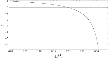
Figure 1: Evolution of $\gamma$, defined in Eq. (65) in the range of values allowed by Eq. (39). As explained in the text, the parameter $\gamma$ controls the amplitude of the squeezed limit of tensor bispectrum in our model, and how much it differs from the same quantity calculated in standard inflationary scenarios.

As anticipated, the momentum dependence for this three-point function is equal to the GR contribution around de Sitter space found in [34], but the overall factor is different. In fact, the amplitude of the bispectrum is proportional to the factor $\gamma$ given by

$$\gamma\,=\,\frac{\left(1-5q_{2}\lambda_{0}^{2}\right)}{\left(1-3q_{2}\lambda_{0}^{2}\right)}\,.$$ (65)

Interestingly, this factor can be well different from one. We can plot $\gamma$ versus $q_{2}\,\lambda_{0}^{2}$, with the latter quantity varying within the range allowed by Eq. (39): we find that when taking the limit

$$q_{2}\,\lambda_{0}^{2}\,\to\,\frac{1}{3}\,,$$ (66)

the factor $\gamma$ is large and negative, as shown in Fig. 1. Notice that the amplitude of the bispectrum gets enhanced in the region where the tensor sound speed becomes small, see Eq. (37).

The tensor bispectrum we evaluated has its maximum contribution in the squeezed limit, as in the case of standard single-field inflationary models. In order to appreciate this feature more clearly, we focus on the two polarization modes defined as

$$\xi^{(s)}(\vec{k})=\tilde{h}_{ij}(\vec{k})e^{*(s)}_{ij}(\vec{k})\,.$$ (67)

We consider the amplitude ${\cal A}^{s_{1}s_{2}s_{3}}$ and the shape of the bispectrum $\langle\xi^{s_{1}}(\vec{k}_{1})\xi^{s_{2}}(\vec{k}_{2})\xi^{s_{3}}(\vec{k}_{3})\rangle$. We have ${\cal A}_{{\cal T}_{1}}^{s_{1}s_{2}s_{3}}=e_{i_{1}j_{1}}^{*(s_{1})}(\vec{k}_{1})e_{i_{2}j_{2}}^{*(s_{2})}(\vec{k}_{2})e_{i_{3}j_{3}}^{*(s_{3})}(\vec{k}_{3}){\cal A}_{i_{1}j_{1}i_{2}j_{2}i_{3}j_{3}}^{{\cal T}_{1}}$ and we obtain

$${\cal A}_{{\cal T}_{1}}^{s_{1}s_{2}s_{3}} = \gamma\tilde{\cal A}(k_{1},k_{2},k_{3})F_{{\cal T}_{1}}^{s_{1}s_{2}s_{3}}(k_{1},k_{2},k_{3}),$$ (68)

where $F_{{\cal T}_{1}}$ coincides with the standard single-field inflation results found in [34]

$$F_{{\cal T}_{1}}^{+++}(k_{1},k_{2},k_{3})=\frac{1}{2}\frac{K^{5}}{64k_{1}^{2}k_{2}^{2}k_{3}^{2}}\bigg{[}K^{3}-4\sum_{i\neq j}k_{i}^{2}k_{j}-4k_{1}k_{2}k_{3}\bigg{]}\,.$$ (69)

We plot in Fig. 2 the amplitude of this first contribution confirming that it peaks in the squeezed limit $k_{3}\rightarrow 0$.

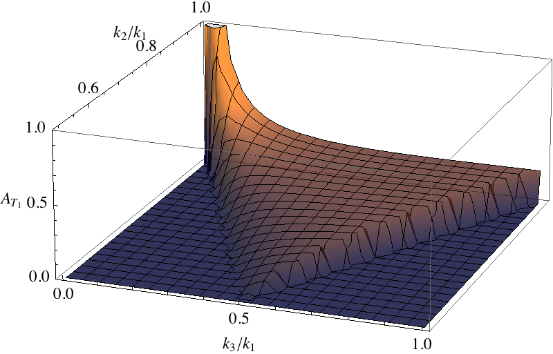
Figure 2: ${\cal A}_{{\cal T}_{1}}^{+++}(1,k_{2}/k_{1},k_{3}/k_{1})(k_{2}/k_{1})^{2}(k_{3}/k_{1})^{2}$ as a function of $k_{2}/k_{1}$ and $k_{3}/k_{1}$. The plot is normalized to unity for equilateral configurations $k_{2}/k_{1}=k_{3}/k_{1}=1$. The contribution to the tensor bispectrum associated with operator ${\cal T}_{1}$ peaks in the squeezed limit.

While the shape is the same as in standard single-field scenarios, the amplitude is modified and can be enhanced through the factor $\gamma$, hence it might be easier to observationally detect.

$\bullet$ The second contribution ${\cal T}_{2}$ is proportional to the mass of the graviton $m_{h}^{2}$ and is distinctive of the scenario that we have considered. Such a contribution is expected when space-reparameterizations are broken, since there is no symmetry that prevents this term. It can be relevant in scenarios in which the size of the graviton mass $|m_{h}^{2}|$ is large (although we will not consider these cases in what follows). Following a procedure similar to the first contribution ${\cal T}_{1}$, we find that

$$\langle\tilde{h}_{i_{1}j_{1}}(\vec{k}_{1})\tilde{h}_{i_{2}j_{2}}(\vec{k}_{2})\tilde{h}_{i_{3}j_{3}}(\vec{k}_{3})\rangle_{{\cal T}_{2}}\,=\,\,(2\pi)^{7}\,\delta^{(3)}\left(\vec{k}_{1}+\vec{k}_{2}+\vec{k}_{3}\right)\,{\cal P}_{h}^{2}\,\frac{{\cal A}^{{\cal T}_{2}}_{i_{1}j_{1}\,i_{2}j_{2}\,i_{3}j_{3}}}{k_{1}^{3}\,k_{2}^{3}\,k_{3}^{3}}\,,$$ (70)

where ${\cal A}^{{\cal T}_{2}}_{i_{1}j_{1}\,i_{2}j_{2}\,i_{3}j_{3}}$ is now given by

$${\cal A}_{i_{1}j_{1}i_{2}j_{2}i_{3}j_{3}}^{{\cal T}_{2}}=\frac{m_{h}^{2}}{H^{2}}\tilde{\mathcal{A}}_{\mathcal{T}_{2}}\Pi_{i_{1}j_{1},lm}(\vec{k}_{1})\Pi_{i_{2}j_{2},mn}(\vec{k}_{2})\Pi_{i_{3}j_{3},nl}(\vec{k}_{3})\,,$$ (71)

with

$$\tilde{\mathcal{A}}_{\mathcal{T}_{2}}(k_{1},k_{2},k_{3})=\frac{1}{48}\biggl{[}k_{1}k_{2}k_{3}+\sum_{i\neq j}k_{i}^{2}k_{j}+(1-\gamma_{E})\sum_{i}k_{i}^{3}\biggr{]}\,,\;\;\;$$ (72)

and $K=k_{1}+k_{2}+k_{3}$.
Like for the contribution $\mathcal{T}_{1}$ we have ${\cal A}_{{\cal T}_{2}}^{s_{1}s_{2}s_{3}}=e_{i_{1}j_{1}}^{*(s_{1})}(\vec{k}_{1})e_{i_{2}j_{2}}^{*(s_{2})}(\vec{k}_{2})e_{i_{3}j_{3}}^{*(s_{3})}(\vec{k}_{3}){\cal A}_{i_{1}j_{1}i_{2}j_{2}i_{3}j_{3}}^{{\cal T}_{2}}$ and we obtain

$${\cal A}_{{\cal T}_{2}}^{s_{1}s_{2}s_{3}} = \tilde{\mathcal{A}}_{\mathcal{T}_{2}}(k_{1},k_{2},k_{3})F_{{\cal T}_{2}}^{s_{1}s_{2}s_{3}}(k_{1},k_{2},k_{3}),$$ (73)

where now $F_{{\cal{T}}_{2}}^{s_{1}s_{2}s_{3}}(k_{1},k_{2},k_{3})$, using the properties of the polarization tensors, results

$$F_{{\cal T}_{2}}^{+++}(k_{1},k_{2},k_{3})=\frac{K^{3}}{64k_{1}^{2}k_{2}^{2}k_{3}^{2}}\bigg{[}K^{3}-4\sum_{i\neq j}k_{i}^{2}k_{j}-4k_{1}k_{2}k_{3}\bigg{]}\,.$$ (74)

In Fig. 3 we plot the non-Gaussian amplitude correspondent to the contribution proportional to the mass of the graviton and we can see that also this contribution has its maximum amplitude in the squeezed limit.

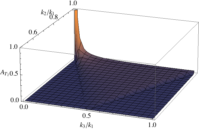
Figure 3: ${\cal A}_{{\cal T}_{2}}^{+++}(1,k_{2}/k_{1},k_{3}/k_{1})(k_{2}/k_{1})^{2}(k_{3}/k_{1})^{2}$ as a function of $k_{2}/k_{1}$ and $k_{3}/k_{1}$. The plot is normalized to unity for equilateral configurations $k_{2}/k_{1}=k_{3}/k_{1}=1$.

Hence, both contributions have their maximum amplitude in the squeezed limit. If we focus our attention in cases where the mass of the graviton is small during inflation, the first contribution is dominant and, as we have seen, it can be enhanced with respect to the similar contribution coming from standard single-field inflationary models. Our starting theory does not show any parity violation feature at the level of the action, so we expect that $F_{{\cal T}_{1},{\cal T}_{2}}^{---}=F_{{\cal T}_{1},{\cal T}_{2}}^{+++}$. Using the properties of the polarization tensors we can also show, from (68) and (71), that $F_{{\cal T}_{1},{\cal T}_{2}}^{++-}(k_{1},k_{2},k_{3})=F_{{\cal T}_{1},{\cal T}_{2}}^{+++}(k_{1},k_{2},-k_{3})$, and again, since we do not have parity violation, we expect that $F_{{\cal T}_{1},{\cal T}_{2}}^{--+}=F_{{\cal T}_{1},{\cal T}_{2}}^{++-}$. It would be interesting to find a mechanism to violate parity at the level of the action and study its features, as it happens in models that involve pseudoscalar fields [50, 51].

We conclude this Section by noticing that our findings so far are relatively straightforward to investigate in our set-up of supersolid inflation with non-minimal coupling with curvature. It would be interesting to examine whether also in the original solid inflation scenario [5] there exist regimes where tensor non-Gaussianity can be parametrically large, and enhanced in squeezed configuration.

4 Dynamics of scalar fluctuations

After analysing the dynamics of tensor modes, we now pass to discuss some aspects of scalar fluctuations in our systems. Features of scalar fluctuations in models of solid and supersolid inflation have already been discussed in some length in the literature – see for example [5, 52]. Scalar fluctuations are characterised by a direction dependent squeezed bispectrum, an enhanced scalar-tensor-tensor three-point function [53], and a slow suppression of any background anisotropies during inflation [29, 30]. We now point out another property that distinguishes our system, and that we find interesting: at leading order in an expansion of $\epsilon_{\phi}$ and $\epsilon_{H}$ (the parameters breaking time-reparameterization and de Sitter symmetry) the dynamics of scalar curvature fluctuation depends (mainly) on $\lambda_{0}$, which is the quantity that characterizes the breaking of space-reparameterizations. This fact has interesting consequences for cosmological observables, like the tensor-to-scalar ratio $r=\mathcal{P}_{h}/\mathcal{P}_{{\cal R}}$.

We adopt a convenient gauge choice for investigating the scalar fluctuations of the fields involved, which we call partially unitary gauge: we set to zero the fluctuation of the scalar $\phi$, while we allow for a non-vanishing scalar component $w$ for the fluctuations of the fields $\sigma^{I}$ responsible for spontaneously breaking space-reparameterizations. At linear order, our expansion of the fields and the spacetime metric around a background configuration reads

$$\phi = \phi(t)\,,$$ (75)

$$\sigma^{I} = \lambda_{0}\,x^{I}+\frac{1}{aH}\,\frac{\lambda_{0}}{\sqrt{-\nabla^{2}}}\,\partial^{I}w\,,$$ (76)

$$ds^{2} = -dt^{2}\,\left(1+2\,N\right)+2\,a^{2}\,\partial_{i}\,B\,dt\,dx^{i}+a^{2}\,\left[\delta_{ij}\,\left(1+2A\right)\right]\,dx^{i}dx^{j}\,.$$ (77)

In our gauge, the scalar fluctuations include the modes $N$, $B$ – which are not dynamical, and correspond to ADM constraints [54] – the mode $A{}$, and the mode $w$. All scalar fluctuations are dimensionless. We are especially interested to investigate the dynamics of $A$, and how it gets affected by the presence of $w$. Notice that in this work for simplicity we do not consider the dynamics of vector modes.

The procedure we follow to determine the action for scalar fluctuations is standard (see e.g. [27]). We substitute our Ansatz for the scalar fields and the metric in our initial action (4), and we expand up to second order in scalar fluctuations. The first order action determines the exact solution for the background level; using the latter, we derive the second order action for the four scalar fluctuations around the background configuration of interest. We discuss quadratic perturbations around the power law configuration described in Section 2.2, which contains, as special case, the expansion around the de Sitter solution studied in Section 2.1.

In general, one gets an intricate quadratic action mixing $A$ and $w$. We show here that there is an interesting corner in the parameter space, characterised by $\epsilon_{H}\ll 1$ and $\epsilon_{\phi}\ll 1$, where the dynamics of scalar fluctuations is relatively easy to investigate. We focus on this regime in this Section, although there might be other ranges of parameter choices that lead to interesting scenarios for the scalar sector. For investigating the system it is convenient to pass to Fourier space. In order to kinetically demix $A$ from $\omega$, it is useful to work with the quantity $\tilde{\omega}$, which connects $\omega$ and $A$ through the relation

$$\omega\,=\,\tilde{\omega}-\frac{12\,q_{2}^{2}\,\lambda_{0}^{4}}{k\,\left(1+q_{2}\lambda_{0}^{2}\right)^{2}}\,A\,.$$ (78)

We first obtain the solution for the constraint equations at leading order in $\epsilon_{H}$, $\epsilon_{\phi}$ that reads

$$N\, = \frac{(1-q_{2}\lambda_{0}^{2})}{(1+q_{2}\lambda_{0}^{2})}\,\frac{\dot{A}}{H}+\left(\epsilon_{H}-\frac{\epsilon_{\phi}}{\left(1+q_{2}\lambda_{0}^{2}\right)}\right)\,\left(\frac{\left(1-q_{2}\lambda_{0}^{2}\right)A}{\left(1+q_{2}\lambda_{0}^{2}\right)}+\frac{a^{2}\,H\,\dot{\tilde{\omega}}}{k}\right)\,+\,{\cal O}\left(\epsilon_{\phi}^{2},\epsilon_{H}^{2}\right)\,,$$ (79)

$$B = -\frac{(1-q_{2}^{2}\lambda_{0}^{4})}{\left(1+q_{2}\lambda_{0}^{2}\right)^{2}}\,\frac{A}{a^{2}\,H}-\frac{12q_{2}^{2}\,\lambda_{0}^{4}\,\dot{A}}{k^{2}\left(1+q_{2}\lambda_{0}^{2}\right)}+{\cal O}\left(\epsilon_{\phi},\epsilon_{H}\right)\,.$$ (80)

It is also not difficult to extend the previous solutions of the constraint equations at higher orders in the $\epsilon$ parameters, but for our purpouse the results of the above expressions are sufficient.

Substituting the constraint conditions, we find that the second order action for the scalars with momentum $k$ results

$$S_{k}^{(S)} = \,\frac{\bar{M}_{Pl}^{2}}{2}\,\int\,dt\,{a^{3}}\,\left[Q^{2}_{A}\,\dot{A}^{2}-\frac{c_{A}^{2}\,k^{2}}{a^{2}}A^{2}-m_{A}^{2}\,A^{2}\right]\,-2\,\Sigma\,H^{2}\,\bar{M}_{Pl}^{2}\,\int\,dt\,a^{3}\,\frac{k}{a\,H}\,\,A\tilde{\omega}$$ (81)

$$+\frac{\bar{M}_{Pl}^{2}}{2}\,\int\,dt\,{a^{3}}\left[Q^{2}_{\tilde{\omega}}\,\dot{\tilde{\omega}}^{2}-\frac{c_{\tilde{\omega}}^{2}\,k^{2}}{a^{2}}\tilde{\omega}^{2}-m_{\tilde{\omega}}^{2}\tilde{\omega}^{2}\right]\,+\,{\cal O}(\epsilon^{2})\,,$$

where

$$\bar{M}_{Pl}^{2} = \left(1-q_{2}\lambda_{0}^{2}\right)\,M_{Pl}^{2}\,,$$ (82)

$${Q}^{2}_{A} = \frac{24\,q_{2}^{2}\lambda_{0}^{4}}{\left(1+q_{2}\lambda_{0}^{2}\right)^{2}}+2\epsilon_{\phi}\,\frac{\left(1-q_{2}\lambda_{0}^{2}\right)}{\left(1+q_{2}\lambda_{0}^{2}\right)^{2}}\,,$$ (83)

$$c_{A}^{2} = \frac{8\,q_{2}^{2}\,\lambda_{0}^{4}}{(1-q_{2}^{2}\lambda_{0}^{4})}+2\epsilon_{\phi}\,\frac{\left(1-q_{2}\lambda_{0}^{2}\right)}{\left(1+q_{2}\lambda_{0}^{2}\right)^{2}}\,,$$ (84)

$$m_{A}^{2} = \frac{12\,H^{2}}{\left(1+q_{2}\lambda_{0}^{2}\right)^{4}\,\left(1-q_{2}\lambda_{0}^{2}\right)}\Big{[}\epsilon_{H}\,\left(1+q_{2}\lambda_{0}^{2}-8q_{2}^{2}\lambda_{0}^{4}+47q_{2}^{4}\lambda_{0}^{8}+87q_{2}^{5}\lambda_{0}^{10}\right)+$$ (85)

$$\hskip 110.96556pt-\epsilon_{\phi}\left(1+q_{2}\lambda_{0}^{2}-5q_{2}^{2}\lambda_{0}^{4}+3q_{2}^{3}\lambda_{0}^{6}+32q_{2}^{4}\lambda_{0}^{8}\right)\Big{]}\,,$$

$$Q^{2}_{\tilde{\omega}} = \frac{2}{\left(1-q_{2}\lambda_{0}^{2}\right)}\left[\epsilon_{H}\left(1+q_{2}\lambda_{0}^{2}\right)-\epsilon_{\phi}\right]\,,$$ (86)

$$c_{\tilde{\omega}}^{2} = \frac{2}{\left(1-q_{2}\lambda_{0}^{2}\right)}\left[\epsilon_{H}\left(1+3q_{2}\lambda_{0}^{2}\right)-\epsilon_{\phi}\right]\,,$$ (87)

$$m^{2}_{\tilde{\omega}} = -4\,Q^{2}_{\omega}\,H^{2}\,,$$ (88)

$$\Sigma = \frac{4}{\left(1+q_{2}\lambda_{0}^{2}\right)^{2}\,\left(1-q_{2}\lambda_{0}^{2}\right)}\,\left[\epsilon_{H}\left(1-q_{2}\lambda_{0}^{2}-11q_{2}^{2}\lambda_{0}^{4}-21q_{2}^{3}\lambda_{0}^{6}\right)-\epsilon_{\phi}\left(1-q_{2}\lambda_{0}^{2}-8q_{2}^{2}\lambda_{0}^{4}\right)\right]\,.$$

Hence we have obtained the quadratic action for scalar fluctuations at leading order in an expansion of small parameters $\epsilon_{\phi}$, $\epsilon_{H}$ (but keeping $\lambda_{0}$ arbitrary).

These results deserve various comments:

• If we focus at zeroth order in an expansion in $\epsilon_{H}$, $\epsilon_{\phi}$, we have only one scalar propagating fluctuation, the mode $A$. The action in this case simplifies to

  $$S_{k}^{A} = \frac{12\,q_{2}^{2}\lambda_{0}^{4}\,\bar{M}_{Pl}^{2}}{\left(1+q_{2}\lambda_{0}^{2}\right)^{2}}\,\int\,dt\,{a^{3}}\,\left[\dot{A}^{2}-\frac{(1+q_{2}\lambda_{0}^{2})}{3(1-q_{2}\lambda_{0}^{2})}\,\frac{k^{2}}{a^{2}}A^{2}\right]\,\,+\,{\cal O}(\epsilon_{\phi},\,\epsilon_{H})\,.$$ (89)

  Hence, the dynamics of $A$ is controlled by the parameter $\lambda_{0}$, characterizing the breaking of space-reparameterization. The sound speed $c_{A}$ for $A$ lies in the interval $1/3\leq c_{A}\leq 2/3$ (since $q_{2}\lambda_{0}^{2}$ is limited within the interval of Eq. (39)). Scalar fluctuations acquire an adiabatic, almost scale-invariant spectrum, as in single-field slow-roll inflation. In this limit, the graviton mass goes to zero and the large-scale anisotropies die out exponentially fast, since tensor modes behave adiabatically.

• When we include first order corrections in the small parameters $\epsilon_{H}$, $\epsilon_{\phi}$, the system starts propagating the second scalar mode $\tilde{\omega}$ besides $A$. In order to avoid ghost-like instabilities associated with $\tilde{\omega}$, we impose

  $$Q_{\omega}^{2}\,\geq\,0\hskip 28.45274pt\Rightarrow\hskip 28.45274pt\epsilon_{H}\,>\,\frac{\epsilon_{\phi}}{1+q_{2}\,\lambda_{0}^{2}}\hskip 28.45274pt\Rightarrow\hskip 28.45274ptm_{h}^{2}\,>\,\frac{8\,\epsilon_{\phi}\,q_{2}\lambda_{0}^{2}}{1-q_{2}^{2}\lambda_{0}^{4}}\,.$$ (90)

  Hence we need a positive mass squared for the tensor modes. The mode $\tilde{\omega}$ is a tachyon with negative mass squared proportional to the Hubble parameter squared, see Eq. (88). On the other hand, such tachyonic instability is not necessarily an insurmountable problem, since in a large-scale limit $k\ll aH$ (where the tachyonic instability becomes important) the coupling of $\tilde{\omega}$ with curvature perturbation is suppressed. At smaller scales, the tachyon instability is less important. It would be interesting to study in full detail possible consequences of this two fields scalar action and possible phenomenological applications, for example along the lines of the recent work [55], also including the effect of interactions controlled by the action at third order in perturbations.

• We can also check what happens ‘turning off’ the parameter controlling the breaking of space-reparameterization. When $\lambda_{0}=0$, at leading order in slow-roll $\epsilon_{\phi}\,=\,\epsilon_{H}$, all the terms in the action containing $\tilde{\omega}$ vanish, and we are left with the standard quadratic action for $A$

  $$S^{A}_{k} = M_{Pl}^{2}\,\epsilon_{\phi}\,\int\,dt\,{a^{3}}\left(\dot{A}^{2}-\frac{k^{2}}{a^{2}}A^{2}\right)\,,$$ (91)

  that reproduces well known results (see e.g. [27]).

• Another potentially interesting case can be obtained selecting $\epsilon_{\phi}\,=\,\epsilon_{H}(1+q_{2}\lambda_{0}^{2})$. This leads to $Q_{\omega}=0$, implying that the mode $\tilde{\omega}$ does not propagate at leading order in perturbations (while it can acquire dynamics at higher orders in perturbative expansion). We will consider this special case in the next subsection.

• We do not study the scalar action expanded at third order in fluctuations since we expect that the study of scalar non-Gaussianity leads to results qualitatively similar to the ones already investigated in [14], namely a direction-dependent squeezed limit for the curvature bispectrum. It would be interesting, on the other hand, to study the amplitude of the the three-point function $\langle h\,A\,A\,\rangle$, given its potentially interesting observational consequences [56, 57, 58].

4.1 Consequences for the tensor-to-scalar ratio

Our findings for the dynamics of quadratic fluctuations in the scalar sector have potentially interesting ramifications for what respects the tensor-to-scalar ratio $r$. We start to explore some aspects of this interesting topic in this subsection. For definiteness, we focus on a specific case of the results we have found above, at leading order in a $\epsilon_{\phi}$, $\epsilon_{H}$ expansion. Our aim it is not to study the dynamics of scalar perturbations in full generality, but instead to exhibit an explicit, simple example where the value of $r$ does not depend on $\epsilon_{H}$, the parameter controlling the breaking of time-reparameterization, but on the parameter $\lambda_{0}$ controlling the breaking of space-translations.

In general, the comoving curvature perturbation ${\cal R}$ is defined in terms of the gauge invariant combination

$${\cal R}\,=\,A+\frac{\dot{A}-H\,N}{\epsilon_{H}\,H}\,.$$ (92)

In the partially unitary gauge we are adopting, see Eqs. (75)-(77), we solved the constraint equations and determined an expression for the non-dynamical variable $N$ in Eq. (79). For simplicity, in this Section we make the following choice to relate $\epsilon_{\phi}$ to $\epsilon_{H}$

$$\epsilon_{\phi}\,=\,\epsilon_{H}\left(1+q_{2}\lambda_{0}^{2}\right)\,.$$ (93)

We also assume that the combination $q_{2}\lambda_{0}^{2}$ is small, although well larger than $\epsilon_{H}$; in other words, we assume the hierarchy

$$\epsilon_{H}\,\ll\,q_{2}\lambda_{0}^{2}\,\ll\,1\,.$$ (94)

A posteriori, we will verify that this condition is the most interesting one for phenomenological applications. Working on this corner of parameter space considerably simplifies the expression (79) for $N$, at leading order in the $\epsilon_{i}$ parameters. Substituting the resulting expression for $N$ in the definition (92), we obtain

$${\cal R}\,=\,A+\frac{2\,q_{2}\,\lambda_{0}^{2}}{\epsilon_{H}\,H\,\left(1+q_{2}\lambda_{0}^{2}\right)}\,\dot{A}\,.$$ (95)

Then, the comoving curvature perturbation depends on $A$ and on its time derivative. In the previous Section, we learned that, at quadratic order, scalar fluctuations are governed by the action (81). Making the choice (93), the perturbation $\tilde{\omega}$ does not propagate, and then can be integrated out: the resulting action describes a single fluctuation $A$ with non-vanishing mass, propagating in a quasi-de Sitter space. The equations of motion for $A$ can then be solved exactly in terms of Hankel functions and, at large scales $k/aH\ll 1$, we find that the solution satisfies the relation

$$\dot{A}\,=\,-\left(1+\frac{28}{3}\,q_{2}\lambda_{0}^{2}\right)\,\epsilon_{H}\,H\,A\,,$$ (96)

which is valid at leading order in $\epsilon_{H}$, and up to first order in an expansion in $q_{2}\lambda_{0}^{2}$. Substituting this result (96) in Eq. (95), we find in the same regime the following proportionality relation between ${\cal R}$ and $A$ at large scales

$${\cal R}\,=\,\Big{(}1-2\,q_{2}\,\lambda_{0}^{2}\Big{)}\,A\,.$$ (97)

We now have all the ingredients to compute the power spectrum for the comoving curvature perturbation ${\cal R}$, following the same steps as done for the tensor spectrum. At large scales we find

$${\cal P}_{\cal R}\,=\,\frac{\sqrt{3}\,H^{2}}{32\,\pi^{2}\,\bar{M}_{Pl}^{2}}\,\frac{1}{q_{2}^{2}\lambda_{0}^{4}}\,,$$ (98)

plus corrections that are small in the limit of small $\epsilon_{H}$ and $q_{2}\lambda_{0}^{2}$. Hence, we learn that the leading contribution to the amplitude of the large scale power spectrum for ${\cal R}$ does not depend on $\epsilon_{H}$, but on the combination $q_{2}\lambda_{0}^{2}$ controlling the breaking of space-reparameterizations.

On the other hand, we recall that the amplitude for the tensor power spectrum is (53)

$${\cal P}_{h}\,=\,\frac{2H^{2}}{\pi^{2}\,\bar{M}_{Pl}^{2}}\frac{\left(1-q_{2}\,\lambda_{0}^{2}\right)^{3/2}}{\left(1-3q_{2}\,\lambda_{0}^{2}\right)^{3/2}}\,\simeq\,\frac{2H^{2}}{\pi^{2}\,\bar{M}_{Pl}^{2}}\,,$$ (99)

where the second equality is valid at zeroth order in an expansion in $q_{2}\,\lambda_{0}^{2}$.

Collecting these results, we find that, at leading (zeroth) order in an expansion in $\epsilon_{\phi}$, $\epsilon_{H}$, and at leading order in $q_{2}\,\lambda_{0}^{2}$, the tensor-to-scalar ratio reads

$$r\,\equiv\,\frac{{\cal P}_{h}}{{\cal P}_{\cal R}}\,=\,\frac{64}{\sqrt{3}}\,{\,q_{2}^{2}\,\lambda_{0}^{4}}\,.$$ (100)

Interestingly, for our choice of hierarchy (94), at leading order $r$ depends only on the parameter $\lambda_{0}$ which spontaneously breaks space-reparameterization, and not at all on $\epsilon_{H}$.

Assuming an upper bound on the tensor-to-scalar ratio $r\leq 0.1$ consistent with the latest CMB constraints [59] allows to extract a limit on the (combination of) parameters $q_{2}\lambda_{0}^{2}$

$$r\leq 0.1\hskip 14.22636pt\Rightarrow\hskip 14.22636ptq_{2}\lambda_{0}^{2}\lesssim 0.05\,,$$ (101)

which motivates our choice (94) of relatively small combination for $q_{2}\lambda_{0}^{2}$. As far as we are aware, this is the first example of inflationary scenario where the tensor-to-scalar ratio is not proportional to $\epsilon_{H}$.

It is important to emphasize that this bound on $q_{2}\lambda_{0}^{2}$ only applies in the particular region of parameter space we examined: there might be other interesting regimes to investigate scalar fluctuations, without imposing a hierarchy as (94), where the tensor-to-scalar ratio shows a different behaviour. However, considering this case for the moment, it is interesting to study the connection among our result and the issue of the Lyth bound. For single-field set-ups where only time-reparameterization is broken, the Lyth bound [60, 61, 62] relates the tensor-to-scalar ratio $r$ with the field excursion $\Delta\phi$ of the inflaton field during inflation. A conservative value of $r$ of order $10^{-2}$ requires that the inflaton field excursion is larger than the Planck scale. Such large-field excursions are dangerous, since it is expected that Planck-scale quantum gravity effects can spoil the flatness of the potential (and the approximate global shift symmetry $\phi\to\phi+const.$) required to sustain a sufficiently large period of inflation. See e.g. the recent [63] for a discussion in the context of string theory. In our set-up, we find that there is no relation between $r$ and the excursion of the field $\phi$: large values of $r$ are compatible with sub-Planckian values of $\phi$, hence avoiding the problem. On the other hand, we do have field excursions on the space-like directions $x^{I}$, associated with $\sigma^{I}$. It is not clear to us whether spatial field excursions should be limited in extensions by some versions or generalisations of the Lyth bound, if one again wishes to avoid symmetry breaking induced by quantum gravity effects. We plan to investigate this topic in a separate paper, also applying the findings of the recent work [64].

5 Conclusions

In this paper we examined the dynamics of cosmological fluctuations in concrete scenarios of supersolid inflation, a framework which spontaneously breaks both space and time reparameterization invariance through the vacuum expectation values of scalar fields driving inflation. We have included a non-minimal coupling of scalar fields with gravity. Our main motivation was to show that this framework can provide qualitatively new features for the dynamics of cosmological fluctuations, which can not be reproduced in frameworks that do not break space-reparameterization, and that can lead to new ways to test the pattern of symmetry breaking during inflation.

We focussed in particular on the tensor sector, including for the first time in this context an analysis of tensor non-Gaussianity. In these scenarios, tensor modes can have a non vanishing mass and a non trivial sound speed. This confirms that primordial gravitational waves can have a blue spectrum, which make them easier to detect at smaller scales [41]. Tensor non-Gaussianity have also distinctive features specifically associated with the pattern of symmetry breaking that we have considered. The third order action for tensor modes has two contributions: one with the same structure as the usual one derived from General Relativity (but with a different overall coefficient), the other is new and specific of our simmetry breaking set-up. We found that the tensor bispectrum is peaked in the squeezed limit, with an amplitude that can be parametrically larger than in standard single-field scenarios of inflation. It would be interesting to investigate whether a large amplitude for the squeezed limit of tensor bispectrum can facilitate the detection of tensor non-Gaussianity, for example inducing large scale anisotropies in the tensor power spectrum, analogously to what happens in the scalar case.

We then analysed the dynamics of scalar perturbations. In general, in this kind of scenarios, two scalar modes propagate and we found that the analysis simplifies considerably at leading order in an expansion in the small parameters breaking time-reparameterization and the de Sitter symmetry – while keeping a larger size for the parameter controlling the breaking of space-reparameterization. At leading order in such expansion, only one scalar mode propagate, which at large scales can be identified with the comoving curvature perturbation ${\cal R}$. At next to leading order, a second mode becomes dynamical, with a tachyonic instability whose effects can be suppressed by the small expansion parameters.

The fact that, at leading order in our expansion, the amplitude of curvature fluctuations is dictated by the parameter controlling the breaking of space-reparameterization is an interesting feature of our set up. As a consequence, in this regime the tensor-to-scalar ratio $r$ is independent of the parameter $\epsilon_{H}$ which controls the breaking of time reparameterization during inflation, as usually happens. Instead, in our case, for the first time we determine scenarios where $r$ depends on quantities controlling the breaking of space-reparameterization. It would be interesting to investigate in more details the consequences of these findings for the effective field theory of inflation, and for issues related to trans-Planckian field excursions and the Lyth bound.

Acknowledgments

We thank Ivonne Zavala for careful reading of the manuscript. The computations performed in this paper have been partially done with the xAct package for Mathematica [65, 66, 67].

Appendix A Appendix A

In this appendix we collect some results useful for expanding the action at second and third order in tensor fluctuations

$$\sqrt{-g} = a^{3}\,,$$ (102)

$$\sqrt{-g}\,g_{ij}\delta^{ij} = 3\,a+\frac{a}{2}\,h_{im}\,h_{mj}-\frac{a}{6}h_{im}h_{ml}h_{lj}\,,$$ (103)

$$\sqrt{-g}\,R = a^{3}\Big{[}12H^{2}+6\dot{H}+\frac{1}{4}\left(\dot{h}_{ij}^{2}-\frac{1}{a^{2}}\left(\partial_{m}h_{ij}\right)^{2}\right)+$$ (104)

$$+\frac{1}{2\,a^{2}}h_{ij}h_{mn}\left(\partial_{j}\partial_{n}h_{im}-\frac{1}{2}\partial_{i}\partial_{j}h_{mn}\right)\Big{]}\,,$$

$$\sqrt{-g}\,G_{ij}\,\delta^{ij} = -3a\left(3H^{2}+2\dot{H}\right)+$$ (105)

$$-\frac{a}{8}\left[3\dot{h}_{ij}\left(\dot{h}_{ij}+4Hh_{ij}\right)+4h_{ij}\left(\ddot{h}_{ij}+h_{ij}\left(3H^{2}+2\dot{H}\right)\right)+\frac{3}{a^{2}}\left(\partial_{l}h_{ij}\right)^{2}\right]$$

$$+{a}\left(\frac{1}{4}\,h_{ij}h_{jm}\ddot{h}_{mi}+\frac{3}{4}Hh_{ij}\dot{h}_{jm}h_{mi}+\frac{\dot{H}}{3}h_{ij}h_{jm}h_{mi}+\frac{H^{2}}{2}h_{ij}h_{jm}h_{mi}\right)$$

$$+\frac{5}{4a}h_{ij}h_{mn}\left(\partial_{j}\partial_{n}h_{im}-\frac{1}{2}\partial_{i}\partial_{j}h_{mn}\right)-\frac{1}{4a}h_{ij}h_{im}\nabla^{2}h_{mj}\,.$$

Latin indexes have been contracted with the 3d Kronecker symbol $\delta_{ij}$.

References

- [1] C. Cheung, P. Creminelli, A. L. Fitzpatrick, J. Kaplan, and L. Senatore, “The Effective Field Theory of Inflation,” JHEP 0803 (2008) 014, arXiv:0709.0293 [hep-th].
- [2] S. Weinberg, “Effective Field Theory for Inflation,” Phys. Rev. D77 (2008) 123541, arXiv:0804.4291 [hep-th].
- [3] F. Piazza and F. Vernizzi, “Effective Field Theory of Cosmological Perturbations,” Class. Quant. Grav. 30 (2013) 214007, arXiv:1307.4350 [hep-th].
- [4] A. Golovnev, V. Mukhanov, and V. Vanchurin, “Vector Inflation,” JCAP 0806 (2008) 009, arXiv:0802.2068 [astro-ph].
- [5] S. Endlich, A. Nicolis, and J. Wang, “Solid Inflation,” JCAP 1310 (2013) 011, arXiv:1210.0569 [hep-th].
- [6] A. Gruzinov, “Elastic inflation,” Phys. Rev. D70 (2004) 063518, arXiv:astro-ph/0404548 [astro-ph].
- [7] B. Himmetoglu, C. R. Contaldi, and M. Peloso, “Instability of anisotropic cosmological solutions supported by vector fields,” Phys. Rev. Lett. 102 (2009) 111301, arXiv:0809.2779 [astro-ph].
- [8] A. Maleknejad and M. M. Sheikh-Jabbari, “Gauge-flation: Inflation From Non-Abelian Gauge Fields,” Phys. Lett. B723 (2013) 224–228, arXiv:1102.1513 [hep-ph].
- [9] A. Maleknejad and M. M. Sheikh-Jabbari, “Non-Abelian Gauge Field Inflation,” Phys. Rev. D84 (2011) 043515, arXiv:1102.1932 [hep-ph].
- [10] P. Adshead and M. Wyman, “Chromo-Natural Inflation: Natural inflation on a steep potential with classical non-Abelian gauge fields,” Phys. Rev. Lett. 108 (2012) 261302, arXiv:1202.2366 [hep-th].
- [11] A. Maleknejad, M. M. Sheikh-Jabbari, and J. Soda, “Gauge Fields and Inflation,” Phys. Rept. 528 (2013) 161–261, arXiv:1212.2921 [hep-th].
- [12] N. Bartolo, S. Matarrese, M. Peloso, and A. Ricciardone, “Anisotropic power spectrum and bispectrum in the mechanism,” Phys. Rev. D87 no. 2, (2013) 023504, arXiv:1210.3257 [astro-ph.CO].
- [13] D. T. Son, “Effective Lagrangian and topological interactions in supersolids,” Phys. Rev. Lett. 94 (2005) 175301, arXiv:cond-mat/0501658 [cond-mat].
- [14] N. Bartolo, D. Cannone, A. Ricciardone, and G. Tasinato, “Distinctive signatures of space-time diffeomorphism breaking in EFT of inflation,” JCAP 1603 no. 03, (2016) 044, arXiv:1511.07414 [astro-ph.CO].
- [15] P. Amaro-Seoane et al., “eLISA/NGO: Astrophysics and cosmology in the gravitational-wave millihertz regime,” GW Notes 6 (2013) 4–110, arXiv:1201.3621 [astro-ph.CO].
- [16] S. Koh, S. Kouwn, O.-K. Kwon, and P. Oh, “Cosmological Perturbations of a Quartet of Scalar Fields with a Spatially Constant Gradient,” Phys. Rev. D88 (2013) 043523, arXiv:1304.7924 [gr-qc].
- [17] G. W. Horndeski, “Second-order scalar-tensor field equations in a four-dimensional space,” Int. J. Theor. Phys. 10 (1974) 363–384.
- [18] E. J. Copeland, A. Padilla, and P. M. Saffin, “The cosmology of the Fab-Four,” JCAP 1212 (2012) 026, arXiv:1208.3373 [hep-th].
- [19] T. Kobayashi, M. Yamaguchi, and J. Yokoyama, “G-inflation: Inflation driven by the Galileon field,” Phys. Rev. Lett. 105 (2010) 231302, arXiv:1008.0603 [hep-th].
- [20] T. Kobayashi, M. Yamaguchi, and J. Yokoyama, “Generalized G-inflation: Inflation with the most general second-order field equations,” Prog. Theor. Phys. 126 (2011) 511–529, arXiv:1105.5723 [hep-th].
- [21] M.-a. Watanabe, S. Kanno, and J. Soda, “Inflationary Universe with Anisotropic Hair,” Phys. Rev. Lett. 102 (2009) 191302, arXiv:0902.2833 [hep-th].
- [22] A. A. Abolhasani, M. Akhshik, R. Emami, and H. Firouzjahi, “Primordial Statistical Anisotropies: The Effective Field Theory Approach,” JCAP 1603 no. 03, (2016) 020, arXiv:1511.03218 [astro-ph.CO].
- [23] F. Lucchin and S. Matarrese, “Power Law Inflation,” Phys. Rev. D32 (1985) 1316.
- [24] A. R. Liddle, “Power Law Inflation With Exponential Potentials,” Phys. Lett. B220 (1989) 502–508.
- [25] D. Cannone, G. Tasinato, and D. Wands, “Generalised tensor fluctuations and inflation,” arXiv:1409.6568 [astro-ph.CO].
- [26] D. Cannone, J.-O. Gong, and G. Tasinato, “Breaking discrete symmetries in the effective field theory of inflation,” JCAP 1508 no. 08, (2015) 003, arXiv:1505.05773 [hep-th].
- [27] J. M. Maldacena, “Non-Gaussian features of primordial fluctuations in single field inflationary models,” JHEP 0305 (2003) 013, arXiv:astro-ph/0210603 [astro-ph].
- [28] A. Higuchi, “Forbidden Mass Range for Spin-2 Field Theory in De Sitter Space-time,” Nucl. Phys. B282 (1987) 397–436.
- [29] N. Bartolo, S. Matarrese, M. Peloso, and A. Ricciardone, “Anisotropy in solid inflation,” JCAP 1308 (2013) 022, arXiv:1306.4160 [astro-ph.CO].
- [30] N. Bartolo, M. Peloso, A. Ricciardone, and C. Unal, “The expected anisotropy in solid inflation,” JCAP 1411 no. 11, (2014) 009, arXiv:1407.8053 [astro-ph.CO].
- [31] M. Akhshik, “Clustering Fossils in Solid Inflation,” JCAP 1505 no. 05, (2015) 043, arXiv:1409.3004 [astro-ph.CO].
- [32] M. Akhshik, R. Emami, H. Firouzjahi, and Y. Wang, “Statistical Anisotropies in Gravitational Waves in Solid Inflation,” JCAP 1409 (2014) 012, arXiv:1405.4179 [astro-ph.CO].
- [33] D. H. Lyth and A. R. Liddle, The primordial density perturbation: Cosmology, inflation and the origin of structure. 2009. http://www.cambridge.org/uk/catalogue/catalogue.asp?isbn=9780521828499.
- [34] X. Gao, T. Kobayashi, M. Yamaguchi, and J. Yokoyama, “Primordial non-Gaussianities of gravitational waves in the most general single-field inflation model,” Phys. Rev. Lett. 107 (2011) 211301, arXiv:1108.3513 [astro-ph.CO].
- [35] D. Green, B. Horn, L. Senatore, and E. Silverstein, “Trapped Inflation,” Phys. Rev. D80 (2009) 063533, arXiv:0902.1006 [hep-th].
- [36] M. M. Anber and L. Sorbo, “Naturally inflating on steep potentials through electromagnetic dissipation,” Phys. Rev. D81 (2010) 043534, arXiv:0908.4089 [hep-th].
- [37] N. Barnaby and M. Peloso, “Large Nongaussianity in Axion Inflation,” Phys. Rev. Lett. 106 (2011) 181301, arXiv:1011.1500 [hep-ph].
- [38] M. Biagetti, M. Fasiello, and A. Riotto, “Enhancing Inflationary Tensor Modes through Spectator Fields,” Phys. Rev. D88 (2013) 103518, arXiv:1305.7241 [astro-ph.CO].
- [39] M. Biagetti, E. Dimastrogiovanni, M. Fasiello, and M. Peloso, “Gravitational Waves and Scalar Perturbations from Spectator Fields,” JCAP 1504 (2015) 011, arXiv:1411.3029 [astro-ph.CO].
- [40] C. Guzzetti, M., N. Bartolo, M. Liguori, and S. Matarrese, “Gravitational waves from inflation,” Riv. Nuovo Cim. 39 no. 9, (2016) 399–495, arXiv:1605.01615 [astro-ph.CO].
- [41] N. Bartolo et al., “Science with the space-based interferometer LISA. IV: Probing inflation with gravitational waves,” arXiv:1610.06481 [astro-ph.CO].
- [42] P. Creminelli, J. Gleyzes, J. Noreña, and F. Vernizzi, “Resilience of the standard predictions for primordial tensor modes,” Phys. Rev. Lett. 113 no. 23, (2014) 231301, arXiv:1407.8439 [astro-ph.CO].
- [43] J. Fumagalli, S. Mooij, and M. Postma, “Tensor power spectrum and disformal transformations,” arXiv:1610.08460 [gr-qc].
- [44] J. D. Bekenstein, “The Relation between physical and gravitational geometry,” Phys. Rev. D48 (1993) 3641–3647, arXiv:gr-qc/9211017 [gr-qc].
- [45] J. M. Maldacena and G. L. Pimentel, “On graviton non-Gaussianities during inflation,” JHEP 09 (2011) 045, arXiv:1104.2846 [hep-th].
- [46] J. Soda, H. Kodama, and M. Nozawa, “Parity Violation in Graviton Non-gaussianity,” JHEP 08 (2011) 067, arXiv:1106.3228 [hep-th].
- [47] J. L. Cook and L. Sorbo, “An inflationary model with small scalar and large tensor nongaussianities,” JCAP 1311 (2013) 047, arXiv:1307.7077 [astro-ph.CO].
- [48] Y. Akita and T. Kobayashi, “Primordial non-Gaussianities of gravitational waves beyond Horndeski theories,” Phys. Rev. D93 no. 4, (2016) 043519, arXiv:1512.01380 [hep-th].
- [49] S. Weinberg, “Quantum contributions to cosmological correlations,” Phys. Rev. D72 (2005) 043514, arXiv:hep-th/0506236 [hep-th].
- [50] M. Shiraishi, A. Ricciardone, and S. Saga, “Parity violation in the CMB bispectrum by a rolling pseudoscalar,” JCAP 1311 (2013) 051, arXiv:1308.6769 [astro-ph.CO].
- [51] R. Namba, M. Peloso, M. Shiraishi, L. Sorbo, and C. Unal, “Scale-dependent gravitational waves from a rolling axion,” JCAP 1601 no. 01, (2016) 041, arXiv:1509.07521 [astro-ph.CO].
- [52] S. Endlich, B. Horn, A. Nicolis, and J. Wang, “Squeezed limit of the solid inflation three-point function,” Phys. Rev. D90 no. 6, (2014) 063506, arXiv:1307.8114 [hep-th].
- [53] E. Dimastrogiovanni, M. Fasiello, D. Jeong, and M. Kamionkowski, “Inflationary tensor fossils in large-scale structure,” JCAP 1412 (2014) 050, arXiv:1407.8204 [astro-ph.CO].
- [54] R. L. Arnowitt, S. Deser, and C. W. Misner, “The Dynamics of general relativity,” Gen. Rel. Grav. 40 (2008) 1997–2027, arXiv:gr-qc/0405109 [gr-qc].
- [55] A. Achúcarro, V. Atal, C. Germani, and G. A. Palma, “Cumulative effects in inflation with ultra-light entropy modes,” arXiv:1607.08609 [astro-ph.CO].
- [56] L. Bordin, P. Creminelli, M. Mirbabayi, and J. Norena, “Tensor Squeezed Limits and the Higuchi Bound,” JCAP 1609 no. 09, (2016) 041, arXiv:1605.08424 [astro-ph.CO].
- [57] D. Jeong and M. Kamionkowski, “Clustering Fossils from the Early Universe,” Phys. Rev. Lett. 108 (2012) 251301, arXiv:1203.0302 [astro-ph.CO].
- [58] G. Domènech, T. Hiramatsu, C. Lin, M. Sasaki, M. Shiraishi, and Y. Wang, “CMB Scale Dependent Non-Gaussianity from Massive Gravity during Inflation,” arXiv:1701.05554 [astro-ph.CO].
- [59] BICEP2, Keck Array Collaboration, P. A. R. Ade et al., “Improved Constraints on Cosmology and Foregrounds from BICEP2 and Keck Array Cosmic Microwave Background Data with Inclusion of 95 GHz Band,” Phys. Rev. Lett. 116 (2016) 031302, arXiv:1510.09217 [astro-ph.CO].
- [60] A. R. Liddle and D. H. Lyth, “COBE, gravitational waves, inflation and extended inflation,” Phys. Lett. B291 (1992) 391–398, arXiv:astro-ph/9208007 [astro-ph].
- [61] L. Boubekeur, “Theoretical bounds on the tensor-to-scalar ratio in the cosmic microwave background,” Phys. Rev. D87 no. 6, (2013) 061301, arXiv:1208.0210 [astro-ph.CO].
- [62] J. Garcia-Bellido, D. Roest, M. Scalisi, and I. Zavala, “Lyth bound of inflation with a tilt,” Phys. Rev. D90 no. 12, (2014) 123539, arXiv:1408.6839 [hep-th].
- [63] S. L. Parameswaran and I. Zavala, “Prospects for Primordial Gravitational Waves in String Inflation,” arXiv:1606.02537 [hep-th].
- [64] D. Klaewer and E. Palti, “Super-Planckian Spatial Field Variations and Quantum Gravity,” arXiv:1610.00010 [hep-th].
- [65] J. M. Martín-García, “http://www.xact.es/.”.
- [66] D. Brizuela, J. M. Martin-Garcia, and G. A. Mena Marugan, “xPert: Computer algebra for metric perturbation theory,” Gen. Rel. Grav. 41 (2009) 2415–2431, arXiv:0807.0824 [gr-qc].
- [67] C. Pitrou, X. Roy, and O. Umeh, “xPand: An algorithm for perturbing homogeneous cosmologies,” Class. Quant. Grav. 30 (2013) 165002, arXiv:1302.6174 [astro-ph.CO].