Essential criteria for efficient pulse amplification via Raman and Brillouin scattering

Abstract

Raman and Brillouin amplification are two schemes for amplifying and compressing short laser pulses in plasma. Analytical models have already been derived for both schemes, but the full consequences of these models are little known or used. Here, we present new criteria that govern the evolution of the attractor solution for the seed pulse in Raman and Brillouin amplification, and show how the initial laser pulses need to be shaped to control the properties of the final amplified seed and improve the amplification efficiency.

Raman (and later Brillouin) scattering and amplification were first discovered in solid-state physics cvraman and also found applications in gases and molecular vibrations armstrong62 ; sen65 ; flora75 ; kaup79 ; menyuk92 as well as non-linear optics lamb1 ; lamb2 . Raman and Brillouin scattering have also been demonstrated in laser-plasma interaction, see e.g. Forslund et al. forslund . Plasma-based compression and amplification of laser pulses via Raman or Brillouin scattering has been proposed to overcome the intensity limitations posed by solid-state optical systems maier66 ; milroy77 ; milroy79 ; capjack82 ; sutyagin ; shvets99 ; andreev06 . In the context of Raman or Brillouin amplification, analytical models have been derived under the assumption that the basic shape of the growing seed pulse does not change during amplification, while its amplitude and duration evolve according to well-defined scaling laws shvets99 ; andreev06 . For Raman amplification (or Brillouin amplification in the weak-coupling regime), this assumption is only correct if the seed pulse has the following properties: (i) pulse amplitude is proportional to the interaction time $t$ shvets98 ; dodin00 ; malkinpop03 ; pingprl ; dino05 , (ii) pulse duration is proportional to $1/t$, or bandwidth proportional to $t$ dodin00 ; malkinpop03 ; pingprl ; dino05 ; kim03 , (iii) pulse energy is proportional to $t$, or inversely proportional to its duration shvets00 ; tsidulko02 ; cheng05 ; renpop08 ; yampolski08 ; malkinprl07 , (iv) the asymptotic “$\pi$-pulse” solution is an attractor solution, i.e. a “not quite ideal” seed pulse will reshape itself into an approximate $\pi$-pulse shape shvets99 ; malkinpop03 ; kim03 ; malkinprl07 ; malkinpop00 ; yampolsky04 ; trines11b ; lehmann1 ; lehmann2 , (v) in multi-dimensional simulations where the pulses have a finite transverse width, the seed pulse acquires a “horseshoe” shape dodin00 ; trines11b ; mardahl02 ; fraiman02 ; balakin03 ; balakin05 ; hur09 ; trines11a ; lehmann3 . Most of the above also applies to Brillouin amplification in the strong-coupling regime andreev06 , although the scalings for the seed pulse duration and amplitude with interaction time are different. In this Letter, we perform the first detailed and systematic study of the full non-linear evolution of the seed pulse for both Raman and Brillouin amplification, and derive novel criteria for the optimal shape of the initial seed pulse before, during and after the interaction, which can be exploited to guide the design of future experiments and maximize their efficiency. At present, the properties of the ideal attractor solution for the seed pulse are not used to optimize the design of Raman or Brillouin amplification experiments.

We define $a_{0}$ and $a_{1}$ to be the scaled envelopes of pump and seed pulse respectively, $a_{0,1}\equiv 8.55\times 10^{-10}g^{1/2}(I_{0,1}\lambda_{0,1}^{2}[\mathrm{Wcm}^{-2}\mu\mathrm{m}^{2}])^{1/2}$, where $g=1$ ($g=1/2$) denotes linear (circular) polarisation. Let $\omega_{0}$ and $n_{cr}$ denote the pump laser frequency and critical density, and $n_{e}$ and $\omega_{pe}$ the background electron density and corresponding plasma frequency. The group velocity of the pump pulse is $v_{g}=c^{2}k_{0}/\omega_{0}=c(1-n_{e}/n_{cr})^{1/2}$ and the electron thermal velocity is $v_{e}=(k_{B}T_{e}/m_{e})^{1/2}$.

For Raman amplification, the envelope equations for pump, seed and plasma wave take the following form shvets99 :

$$(\partial/\partial t\pm v_{g}\partial/\partial x)a_{0,1} =\mp i\Gamma_{R}a_{1,0}b^{(*)},$$ (1)

$$(\partial/\partial t+3v_{e}^{2}(k/\omega_{pe})\partial/\partial x)b =-i\Gamma_{R}a_{0}a_{1}^{*},$$ (2)

where $\Gamma_{R}a_{0}$ denotes the Raman backscattering growth rate in homogeneous plasma and $b\equiv\alpha_{R}\delta n_{e}/n_{e}$ with $\delta n_{e}$ the envelope of the electron density fluctuations driven by the beating of pump and seed pulses, and $\alpha_{R}$ to be determined. Comparing these equations to the envelope equations by Forslund et al. forslund yields $\Gamma_{R}\alpha_{R}=\omega_{pe}^{2}/(4\omega_{0})$ and $\Gamma_{R}/\alpha_{R}=c^{2}k^{2}/(4g\omega_{pe})$, where $k\approx 2k_{0}\approx 2\omega_{0}/c$ is the wave number of the RBS Langmuir wave (for $\omega_{pe}\ll\omega_{0}$). Then $\Gamma_{R}=[\omega_{0}\omega_{pe}/(4g)]^{1/2}$ and $\alpha_{R}=\sqrt{g}(\omega_{pe}/\omega_{0})^{3/2}/2$, with (1)-(2) valid for $a_{0}<a_{wb}=\alpha_{R}/\sqrt{2}$ shvets99 .

Following Malkin, Shvets and Fisch shvets99 , or Menyuk, Levi and Winternitz menyuk92 , we define $\zeta=x/c+t$, $t^{\prime}=\Gamma_{R}^{2}a_{00}^{2}t$ and $\xi=2\sqrt{\zeta t^{\prime}}$ where $a_{00}$ denotes the pump pulse amplitude. Attractor solutions to the above system can then be obtained in terms of $\xi$ alone. In particular, the first peak of the growing seed pulse can be approximated by $a_{1}(\zeta,t^{\prime})\approx(2t^{\prime}/\Gamma_{R}\xi)\partial u(\xi)/\partial\xi$ where $u(\xi)=2\sqrt{2}\arctan[\epsilon\exp(\xi)/(4\sqrt{2\pi\xi})]$, with $\epsilon<0.1$ depending on the initial seed pulse B-integral. The function $\partial u(\xi)/\partial\xi$ has an amplitude $A\approx 1.29$ and a width $\Delta\xi\approx 2.65$, mostly independent of $\epsilon$, while the position of its maximum, $\xi_{M}$, obeys $5<\xi_{M}<7$ for practical values of $\epsilon$ shvets99 ; dodin00 . Let $\Delta\zeta$ denote the width of the first peak of $a_{1}(\zeta,t^{\prime})$ for fixed $t^{\prime}$ and let $\xi_{1,2}=\xi_{M}\pm\Delta\xi/2$. Then $\xi_{M}\Delta\xi=(\xi_{2}^{2}-\xi_{1}^{2})/2=2t^{\prime}\Delta\zeta$. For $\xi=\xi_{M}$, we find that $||a_{1}||=2At^{\prime}/(\Gamma_{R}\xi_{M})$, $\Delta\zeta=\xi_{M}\Delta\xi/(2t^{\prime})$. We consider pump and seed pulses with durations $\tau_{0}$ and $\tau_{1}$ (after amplification), and setting $\Delta\zeta=\tau_{1}$ and $t=\tau_{0}/2$ (for an interaction time $t$, the counter-propagating seed pulse consumes $2t$ of pump pulse), we find:

$$\Gamma_{R}^{2}a_{00}^{2}\tau_{0}\tau_{1} =\xi_{M}\Delta\xi\approx 15,$$ (3)

$$\Gamma_{R}||a_{1}||\tau_{1} =A\Delta\xi\approx 3.4.$$ (4)

The asymptotic energy transfer efficiency for the first peak is then given by $\eta=||a_{1}||^{2}\tau_{1}(t)/(2a_{0}^{2}t)=A^{2}\Delta\xi/\xi_{M}\approx 4.4/\xi_{M}$. Thus, $\eta$ is constant for a given configuration, and decreases with increasing $\xi_{M}$. We confirm these predictions in our simulations below.

The purpose of these equations is as follows. Eq. (3) allows one to derive scalings for the seed pulse duration $\tau_{1}(t)$ and amplitude $a_{1}(t)$, and also to tune these parameters via the intensity of the pump pulse trines11b . Eq. (4) provides a relationship between seed pulse duration and amplitude that does not depend on the pump pulse at all (the only combination of $a_{1}$ and $\tau_{1}$ with this property). This is important for the tailoring of the initial seed pulse in experiments: $\tau_{1}(0)$ and $a_{1}(0)$ are not independent parameters, but should obey Eq. (4) for optimal energy transfer, otherwise the seed pulse will first reshape itself and only be amplified after that yampolsky04 ; lehmann1 ; lehmann2 ; trines11b , reducing the amplification efficiency.

Brillouin scattering in the so-called weak-coupling regime milroy79 ; sutyagin ; forslund ; cohen79 ; cohen01 ; williams is very similar to Raman scattering and can be treated in the same way. We introduce $\omega_{pi}=\omega_{pe}\sqrt{Zm_{e}/m_{i}}$ and $c_{s}=v_{e}\sqrt{Zm_{e}/m_{i}}$. For $a_{00}^{2}<8g(\omega_{0}/\omega_{pe})^{2}c_{s}v_{e}^{2}/c^{3}$, the electron pressure is the dominant restoring force and the plasma wave dispersion is not significantly affected by the beating between pump and seed pulses. In that case one can reuse equations (1)-(2) and only needs to replace $3v_{e}^{2}(k/\omega_{pe})$ by $c_{s}$ in (2). For backward Brillouin scattering, the ion-acoustic wave has wave number $k_{s}=2k_{0}$ and frequency $\omega_{s}=c_{s}k_{s}=2c_{s}k_{0}$. Then we find $\Gamma_{B}\alpha_{B}=\omega_{pe}^{2}/(4\omega_{0})$ and $\Gamma_{B}/\alpha_{B}=c^{2}c_{s}^{2}k_{s}^{2}/(4g\omega_{s}v_{e}^{2})$, leading to $\Gamma_{B}=c\omega_{pe}\omega_{s}/(4v_{e}\sqrt{g\omega_{0}\omega_{s}})$ and $\alpha_{B}=\sqrt{g}v_{e}\omega_{pe}/(c\sqrt{\omega_{0}\omega_{s}})$. After substituting $\Gamma_{B}$, $\alpha_{B}$ for $\Gamma_{R}$, $\alpha_{R}$, all the above results for Raman amplification also apply to the weak-coupling Brillouin case, including Eqns. (3) and (4), the wave breaking threshold $a_{wb}=\alpha_{B}/\sqrt{2}$, the numerical constants $5<\xi_{M}<7$, $\Delta\xi\approx 2.65$ and $A\approx 1.29$, and the seed pulse scalings.

For $a_{00}^{2}>8g(\omega_{0}/\omega_{pe})^{2}c_{s}v_{e}^{2}/c^{3}$ or $\Gamma a_{0}/\omega_{0}>c_{s}/c$, the ponderomotive pressure from the beating between pump and seed pulses will take over from the thermal pressure as the primary restoring force for the ion-acoustic wave. In this regime, called strong-coupling (sc) Brillouin scattering, the equation for the plasma wave becomes andreev06 :

$$\partial^{2}b/\partial t^{2}=-\alpha_{sc}c^{2}k^{2}\omega_{pi}^{2}/(2g\omega_{pe}^{2})a_{0}a_{1}=-\Gamma_{sc}^{2}a_{0}a_{1}.$$ (5)

From (1) and (5) and using $k=2k_{0}=2\omega_{0}v_{g}/c^{2}$ as before, we find: $\Gamma_{sc}\alpha_{sc}=\omega_{pe}^{2}/(4\omega_{0})$ and $\ \Gamma_{sc}^{2}/\alpha_{sc}=c^{2}k^{2}\omega_{pi}^{2}/(2g\omega_{pe}^{2})$. This yields forslund ; huller ; andreev06 :

$$\Gamma_{sc} =[(v_{g}/c)^{2}\omega_{pi}^{2}\omega_{0}/(2g)]^{1/3}=(2\omega_{s}\Gamma_{B}^{2})^{1/3},$$ (6)

$$\Omega_{sc} =\omega_{sc}+i\gamma_{sc}=[(1+i\sqrt{3})/2]\Gamma_{sc}a_{00}^{2/3},$$ (7)

where $\omega_{sc}$ and $\gamma_{sc}$ denote the frequency and growth rate of the ion-acoustic wave. Following the approach by Andreev et al. andreev06 , we define $t^{\prime}=\Gamma_{sc}a_{00}^{2/3}t$, $\zeta=\Gamma_{sc}a_{00}^{2/3}(t+x/v_{g})$ and $\xi=\zeta\sqrt{t^{\prime}}$. Again, attractor solutions to the system (1) and (5) can be obtained in terms of $\xi$ alone. In particular, the resulting seed pulse will scale as $a_{1}(\zeta,t^{\prime})=a_{00}(t^{\prime})^{3/4}f(\xi)$ where $f(\xi)$ has a fixed duration $\Delta\xi\approx 3.3$ and an amplitude $A\approx 0.62$ andreev06 ; lehmann2 . Using $\Delta\xi=(\Delta\zeta)\sqrt{t^{\prime}}$ for fixed $t^{\prime}$, $||a_{1}||=a_{00}A(\Delta\xi/\Delta\zeta)^{3/2}$ and inserting $\Delta\zeta=\Gamma_{sc}a_{00}^{2/3}\tau_{1}$ and $t^{\prime}=\Gamma_{sc}a_{00}^{2/3}\tau_{0}/2$ for pump and seed pulses with durations $\tau_{0}$ and $\tau_{1}$ into $\Delta\xi$ yields:

$$\Gamma_{sc}^{3}a_{00}^{2}\tau_{0}\tau_{1}^{2} =2(\Delta\xi)^{2}\approx 22,$$ (8)

$$\Gamma_{sc}^{3}||a_{1}||^{2}\tau_{1}^{3} =A^{2}(\Delta\xi)^{3}\approx 13.8.$$ (9)

The scaling for the seed pulse duration is then $\tau_{1}(t)=\Delta\xi/(\Gamma_{sc}^{3/2}a_{00}t^{1/2})$, and the asymptotic efficiency is $\eta=a_{1}^{2}(t)\tau_{1}(t)/(2a_{00}^{2}t)=A^{2}\Delta\xi/2\approx 0.63$. The role of (8) and (9) matches that of (3) and (4) for Raman amplification.

To verify the validity of Eqns. (4) and (9), we have carried out one-dimensional particle-in-cell simulations using the codes XOOPIC xoopic and OSIRIS osiris . We used a long pump laser beam with constant amplitude $a_{0}$ and wave length $\lambda_{0}=1\ \mu$m ($\omega_{0}=2\pi c/\lambda_{0}$, $n_{cr}=\varepsilon_{0}m_{e}\omega_{0}^{2}/e^{2}$), a long plasma column with constant electron density $n_{0}$ and plasma frequency $\omega_{pe}$, and a seed pulse with initial amplitude $a_{1}(0)=a_{0}$ and duration $\tau_{1}(0)$. For the Raman simulations, we used a plasma density corresponding to $\omega_{pe}/\omega_{0}=1/15$, pump laser amplitudes $a_{wb}/4$, $a_{wb}/2$, $3a_{wb}/4$, $a_{wb}$ and $2a_{wb}$, with $a_{wb}$ adjusted for each plasma density, and pump pulse durations up to $2\times 10^{5}/\omega_{0}\approx 112$ picoseconds. We use $\tau_{1}(0)/\tau_{R}=0.1$, 0.5, 1.0 and 2.0, where $\tau_{R}[\mathrm{s}]=4.22\times 10^{-6}\lambda_{0}[\mu\mathrm{m}](n_{e}/n_{cr})^{-1/4}(I_{1}\lambda_{1}^{2}[\mathrm{Wcm}^{-2}\mu\mathrm{m}^{2}])^{-1/2}$ is taken from (4). For the Brillouin simulations, we used $m_{i}/(Zm_{e})=1836$, a plasma density $n_{e}=0.3n_{cr}$ and pump amplitudes $a_{0}=0.0085$, 0.027 and 0.085, corresponding to $10^{14}$, $10^{15}$ and $10^{16}$ W cm^-2, and pump pulse durations of 11.4 ps, 3.8 ps and 1.1 ps respectively. We use $\tau_{1}(0)/\tau_{B}=0.1$, 0.2, 0.5, 1.0, 2.0 and 5.0, where $\tau_{B}[\mathrm{s}]=1.78\times 10^{-9}\lambda_{0}[\mu\mathrm{m}][(Zm_{e}/m_{i})(n_{e}/n_{cr})(1-n_{e}/n_{cr})(I_{1}\lambda_{1}^{2}[\mathrm{Wcm}^{-2}\mu\mathrm{m}^{2}])]^{-1/3}$ is taken from (9). The parameters of the simulations are discussed at length in the Supplementary Information supp .

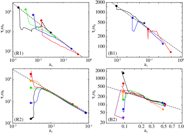
Figure 1: Evolution of duration ($\tau_{1}$) versus peak amplitude ($a_{1}$) of Raman (R1,R2) and sc-Brillouin (B1,B2) amplified pulses for different pump amplitudes (R1,B1) or initial seed durations (R2,B2), demonstrating the attractor nature of the ideal solutions. R1: $n_{0}/n_{cr}=0.0044$, and $a_{0}/a_{wb}=0.25$ (black), 0.5 (green), 1.0 (blue) and 2.0 (red), with initial seed amplitude $a_{1}=a_{0}$ for each case. B1: $n_{0}/n_{cr}=0.3$, and $a_{0}=0.0085$ (black), 0.027 (blue) and 0.085 (red); again, $a_{1}=a_{0}$. R2: $n_{0}/n_{cr}=0.0044$, $a_{1}=a_{0}=0.75a_{wb}$. The initial durations of the seed pulse are $\tau_{1}/\tau_{R}=0.02$ (black), 0.1 (blue) 0.5 (green), 1.0 (orange) and 2.0 (red). B2: $n_{0}/n_{cr}=0.3$, and pump and seed amplitudes of $a_{0}=a_{1}=0.085$. The initial durations of the seed pulse are $\tau_{1}/\tau_{B}=0.1$ (purple), 0.2 (blue), 0.5 (green), 1.0 (orange), 2.0 (red), and 5.0 (black). The dashed lines correspond to Eqns. (4) for Raman and (9) for sc-Brillouin respectively.

In Figure 1, we show the evolution of $\omega_{0}\tau_{1}$ versus $a_{1}$ for simulations of Raman (left) and Brillouin (right) amplification, to demonstrate the “attractor” nature of the optimal seed pulse solutions (4) and (9). The dashed lines in each frame represent Eqns. (4) and (9) evaluated for these cases. The top two frames show ($\omega_{0}\tau_{1}$,$a_{1}$) for various initial pump and seed pulse intensities, where $\tau_{1}(0)=\tau_{R}$ or $\tau_{1}(0)=\tau_{B}$ in each simulation. We find that the evolving seed pulses closely follow the analytical predictions, irrespective of the pump intensity chosen in the simulations, proving that the predictions by (4) and (9) for Raman or Brillouin amplification represent “attractor” solutions and remain valid over a wide range of pulse intensities. For $a_{1}(t)$ and $\tau_{1}(t)$, we find that $a_{1}(t)\propto t$ and $\tau_{1}(t)\propto 1/t$ for Raman amplification and $a_{1}(t)\propto t^{3/4}$ and $\tau_{1}(t)\propto t^{-1/2}$ for sc-Brillouin, although minor aberrations from these scalings were found at the highest pulse intensities due to non-linear effects not covered by the three-wave models, e.g. when the seed pulse becomes powerful enough to drive a wakefield. The bottom two frames show ($\omega_{0}\tau_{1}$,$a_{1}$) for fixed pulse intensities, while the initial pulse duration was moved away from the analytical predictions. We find that in each case the seed pulse first evolves until the pair ($\omega_{0}\tau_{1}$,$a_{1}$) matches (4) or (9), and then amplifies as dictated by these equations. This specific behaviour was found in all our simulation results, irrespective of the plasma density or pump pulse intensity we used. This proves the following: (i) the $\pi$-pulse solution for Raman and its Brillouin equivalent are indeed attractors, as predicted shvets99 ; andreev06 , and (ii) changing the initial seed pulse duration has no significant effect on the end result, so $\tau_{1}(0)$ should not be treated as a free parameter. The free parameters for both Raman and Brillouin amplification are the pump wave length $\lambda_{0}$ and the density ratio $n_{0}/n_{cr}$; once these two are chosen, the position of the attractor $(\tau_{1},a_{1})$ curve is completely determined by (4) or (9). The intensities of the pulses determine the speed at which the seed pulse evolves, but not the trajectory of $(\tau_{1}(t),a_{1}(t))$.

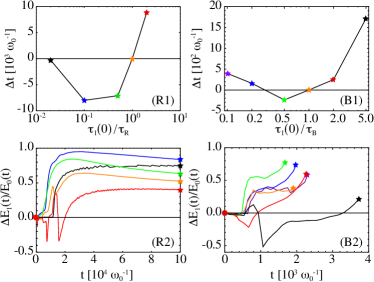
Figure 2: (R1,B1): temporal delay $\Delta t$ in reaching a given intensity amplification level $(25\times I_{\mathrm{pump}})$ for seed pulses with various initial durations, for the same cases as shown in frames (R2,B2) of Figure 1. (R2,B2): efficiency of the amplification process for these same cases; $\Delta E_{1}$ is the seed energy gain, $E_{0}$ is the absorbed pump energy.

In Figure 2(R1,B1), we show the time needed for seed pulses with different initial durations to reach a given intensity $(25\times I_{\mathrm{pump}})$, for the same cases as shown in frames (R2,B2) of Figure 1. We find that amplification is optimal when $0.2<\tau_{1}(0)/\tau_{R,B}<0.5$, ($\tau_{R,B}$ given by (4) or (9)) while significant delays are incurred for $\tau_{1}(0)/\tau_{R,B}>1$ or $<0.2$. In Figure 2(R2,B2) we show the efficiency of the amplification process for these same cases ($\Delta E_{1}\equiv E_{1}(t)-E_{1}(0)$, so $\Delta E_{1}<0$ means that the seed pulse is losing energy rather than gaining). Unsurprisingly, a longer delay in amplification is always accompanied by a lower efficiency. For Raman amplification in particular, we also find that (i) the asymptotic efficiency is mostly constant, (ii) the cases showing the longest delay also exhibit the lowest asymptotic efficiency. This corresponds to the notion that the Raman efficiency is $\eta\approx 4.4/\xi_{M}$ (see above) and that $\xi_{M}$ increases for non-ideal initial seed pulses that incur longer delays, in line with predictions for $\xi_{M}$ in Ref. shvets99 . So a poorly chosen initial seed pulse duration will affect the entire amplification process, not just the initial stages. Also, the longest delays correspond to an interaction length of several mm, longer than what is used in many experiments ren07 ; renpop08 ; kirkwood07 ; ping09 . This highlights the need to choose the initial seed pulse parameters according to Eqns. (4) and (9).

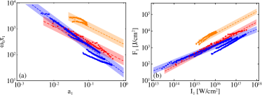
Figure 3: Left: map of $(a_{1},\tau_{1})$ of successfully amplified seed pulses via Raman amplification (blue), sc-Brillouin amplification at over-quarter-critical densities (red) and sc-Brillouin amplification at sub-quarter-critical densities (orange). The points are taken from 1-D PIC simulations while the shaded areas indicate predictions by Eqns. (4) and (9). Right: The same data shown on the left is presented in a map of seed fluence versus seed intensity, for 1 $\mu$m pump pulse wave length.

To make the connection with past Raman or Brillouin amplification experiments, we have applied our findings to the initial conditions of various Raman ren07 ; renpop08 ; kirkwood07 ; ping09 and Brillouin amplification experiments lancia10 ; lancia16 . For the initial seed pulses in the Raman experiments, we find that $\Gamma_{R}a_{1}\tau_{1}=0.13$ ren07 ; renpop08 , 0.22 kirkwood07 , or 0.86 ping09 , well below our value of 3.4. For the Brillouin experiments, we find that $\Gamma_{sc}^{3}a_{1}^{2}\tau_{1}^{3}=8.6$ lancia10 or 1.31 lancia16 again below our value of 13.8. Interestingly, the output pulse after the first pass of the experiments by Ren et al. ren07 ; renpop08 has $\Gamma_{R}a_{1}\tau_{1}\approx 3.5$, matching our predictions. Thus, future experiments need either more powerful seed pulses (up to two orders of magnitude extra power for Raman and one order for Brillouin, for similar duration) or longer interaction distances, to allow the pulses time to reshape themselves. We also note that the experiments with the biggest energy gain, Refs. ren07 ; lancia10 are also the ones using pulses that match our predictions most closely.

In Figure 3, we compare 1-D simulations of Raman amplification at $0.0025<n_{0}/n_{cr}<0.01$ (blue) and sc-Brillouin amplification at $m_{i}/(Zm_{e})=1836$, $0.275<n_{0}/n_{cr}=0.325$ (red) and $0.0075<n_{0}/n_{cr}=0.0125$ (orange). The density ranges have been chosen to minimize the impact of unwanted instabilities trines11a . The dots mark the simulation results, while the shaded areas mark the predictions by Eqns. (4) and (9). The left frame shows $\tau_{1}$ versus $a_{1}$ for the amplified seed; the right frame shows the energy flux $F_{1}=I_{1}\tau_{1}$ versus intensity $I_{1}$ for the same cases. All simulation points lie within the theoretically predicted shaded regions, highlighting the robustness of (4) and (9) for a broad range of parameters. Note that Raman and high-density sc-Brillouin produce the shortest pulses and highest intensities. Low-density Brillouin amplification reaches lower peak intensities but yields the highest pulse fluence because of longer pulse durations. These results serve as an important guide when choosing not only the laser and plasma parameters, but also the preferred amplification scheme when designing an experiment to obtain a desired output pulse.

Finally, we applied our findings to the results of previously published 2-D Raman and Brillouin simulations trines11a ; vieira16 , where both the seed pulse amplitude and duration depend on the transverse coordinate $r$. We found that even if $a_{1}(r)$ and $\tau_{1}(r)$ depend on $r$ individually, they still obey Eqns. (4) and (9). For example, for seed pulses with a Gaussian envelope, $a_{1}(x_{2})\propto\exp(-r^{2}/w_{0}^{2})$, this results in a horseshoe envelope $\tau_{1}(r)\propto\exp(r^{2}/w_{0}^{2})$, as seen in Refs. dodin00 ; trines11b ; mardahl02 ; fraiman02 ; balakin03 ; balakin05 ; hur09 ; trines11a ; lehmann3 . For donut-shaped seed pulses with orbital angular momentum, this even results in a “double horseshoe” envelope vieira16 . These findings are discussed at length in the Supplementary Material supp

We have explored the full non-linear evolution of the seed pulse in Raman and Brillouin amplification, and derived essential criteria governing $a_{1}(t)$ and $\tau_{1}(t)$, in particular specific products of $a_{1}$ and $\tau_{1}$ that are independent of the pump pulse properties. We have proved the validity of these criteria in 1-D and 2-D particle-in-cell simulations. Furthermore, we have demonstrated the importance of choosing the initial seed duration wisely: a non-optimal value for this parameter (far from the ideal attractor solution) will delay amplification of the seed pulse and reduce efficiency. In relation to experiments on parametric amplification, our results provide unique criteria for their design, and novel predictions for the properties of the amplified seed pulse, and advice on which scheme to choose to obtain the desired end result. Since the ideal amplified seed pulse assumes the shape of a cnoidal wave armstrong62 ; shvets99 ; andreev06 , our results also explain the “bursty behaviour” observed in Brillouin scattering weber06 ; weber11 , as the scattered radiation assumes a very similar shape. Since the equations for Raman scattering in solid-state physics or non-linear optics have a shape similar to Eqns. (1)-(2) (see Refs. armstrong62 ; sen65 ; flora75 ; kaup79 ; menyuk92 ; lamb1 ; lamb2 ) our results will be useful for Raman and Brillouin scattering in general (not just in plasma), or to any optical three-wave process with Kerr or $\chi^{(3)}$ non-linearity and counter-propagating pulses, ensuring a wide range of applications.

Parameters of the numerical simulations. For the simulations in the main manuscript, we have used the particle-in-cell codes XOOPIC xoopic and OSIRIS osiris . The parameters are discussed in detail here. We distinguish numerical parameters (spatial resolution, time step, number of particles per grid cell) and physical parameters (laser pulse duration, spot diameter and amplitude, plasma density, plasma species, laser-plasma interaction length, etc.)

Both the Raman and Brillouin runs that have been performed with for figures 1 and 2 of maion manuscript have been done using a moving simulation window. This window followed the seed pulse, while the pump pulse was brought into the simulation box via a time-dependent boundary condition.

The numerical parameters were as follows. For the Raman runs (frames R1 and R2 in both figures of the main manuscript), the spatial resolution was 50 points per pump laser wavelength (i.e. $dx=21$ nm). The time step was given by $dt=0.95dx/c$. The number of particles was 100 particles per cell per species. The interpolation between particles and grid was done using quadratic splines. Ions were treated as an immobile background. For the Brillouin runs (frames B1 and B2 in both figures of the main manuscript), the spatial resolution was $dx=0.5\lambda_{D}$, where $\lambda_{D}$ is the Debye length. This corresponds to about 220 points per pump laser wavelength (i.e. $dx=4.8$ nm). The time step was again $dt=0.95dx/c$. The number of particles was again 100 particles per cell per species, and cubic splines were used for interpolation.

The physical parameters were as follows. The pump laser wave length was 1 $\mu$m for both the Raman and Brillouin simulations. The seed laser wave length for the Raman simulations was 1.07 $\mu$m, chosen to ensure that $\omega_{1}=\omega_{0}-\omega_{pe}$. The seed laser wave length for the Brillouin runs was 1 $\mu$m. (This hardly matters since the frequency difference between pump and seed pulses in Brillouin amplification is considerably less than the seed pulse bandwidth.) For the Brillouin runs in figure 1, frames B1, the interaction length was about $2\times 10^{4}c/\omega_{0}$, $8\times 10^{3}c/\omega_{0}$, and $2\times 10^{3}c/\omega_{0}$ for the simulations with pump intensity $10^{14}$, $10^{15}$ and $10^{16}$ W/cm² simulations of frame B1. The interaction lengths for the simulations in figure 1, frame B2, are $2\times 10^{3}c/\omega_{0}$ in each case. This corresponds to an interaction distance of 335 micron, or a 2.2 ps pump pulse duration. The interaction distance for the Raman runs in figure 1 was up to $10^{5}c/\omega_{0}$ or up to $16$ mm in each case.

The interaction distance for the simulations displayed in figure 2 is up to $10^{5}c/\omega_{0}$ for the Raman runs, and up to $2\times 10^{3}c/\omega_{0}$ for the Brillouin runs.

The plasma density was chosen to be $n_{e}=n_{cr}/225$ for the Raman simulations, and $n_{e}=0.3n_{cr}$ for the Brillouin simulations. The plasma electron temperature was chosen to be 1 eV for the Raman simulations and 500 eV for the Brillouin simulations.

Transverse effects. In a multi-dimensional setting, the amplitude $a1$ and duration $\tau_{1}$ of the growing seed laser pulse will of course depend on the transverse coordinate $x_{2}$. The same holds true for the location of the seed pulse maximum, $\tau_{M}$. This leaves an imprint on the full shape of the envelope when parametric amplification is studied in more than one dimension.

From Equations (4) and (9), we find that the $x_{2}$-dependence of the amplitude $a_{1}$ also induces an $x_{2}$-dependence of the duration $\tau_{1}$, even for fixed $t$. For example, for seed pulses with a Gaussian envelope, $a_{1}(x_{2})\propto\exp(-x_{2}^{2}/w_{0}^{2})$, this results in a horseshoe envelope $\tau_{1}(x_{2})\propto\exp(x_{2}^{2}/w_{0}^{2})$ dodin00 ; trines11b ; mardahl02 ; fraiman02 ; balakin03 ; balakin05 ; hur09 ; trines11a ; lehmann3 . For donut-shaped seed pulses with orbital angular momentum, this even results in a “double horseshoe” envelope vieira16 . We will verify such horseshoe seed pulse shapes against Eqns. (4) and (9) here.

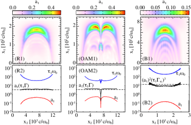
Figure 4: Analyzing the curved shape of the amplified seed pulse for Raman (R) and Raman with OAM (OAM) and Brillouin (B) amplification in multi-dimensional simulations. The top frames show the amplitude envelopes of the amplified seeds. The bottom frames show $a_{1}(x_{2})$ (red) and $\omega_{0}\tau_{1}(x_{2})$ (blue) versus the transverse coordinate $x_{2}$. The products $a_{1}(x_{2})\Gamma_{R}\tau_{1}(x_{2})$ (R,OAM) and $a_{1}^{2}(x_{2})[\Gamma_{sc}\tau_{1}(x_{2})]^{3}$ (B), given by black curves, are then verified against Eqns.(4) and (9) (dashed lines).

In Figure 4, we verify the horseshoe shape of seed pulses after amplification. Here, we present the analysis of a 2-D Raman simulation (R), taken from Ref. trines11a , Figure 2a, a 3-D Raman simulation with orbital angular momentum and a doughnut-shaped seed pulse intensity envelope (OAM), taken from Ref. vieira16 , Figure 1a and 2a, and a 2-D sc-Brillouin simulation (B), using $m_{i}/(Zm_{e})=1836$, $n_{0}/n_{cr}=0.3$ and $a_{0}=0.027$. Frames R1, OAM1 and B1 show the vector potential envelopes for these pulses. Frames R2, OAM2 and B2 show $a_{1}(x_{2})$, $\omega_{0}\tau_{1}(x_{2})$ and $\Gamma_{R}a_{1}(x_{2})\tau_{1}(x_{2})$ and $A\Delta\xi\approx 3.4$ (R2,OAM2) or $\Gamma_{sc}^{3}a_{1}^{2}(x_{2})\tau_{1}^{3}(x_{2})$ and $A^{2}\Delta\xi^{3}\approx 13.8$ (B2), all versus transverse coordinate $x_{2}$. In all cases, the curved shape of the seed pulse is well described by Eqns. (4) or (9). Even for strange pulse envelope shapes, like the “donut” shape of the pulse with OAM, the relationships between pulse amplitude and duration still hold. The presence or absence of parastic instabilities does not have much of an influence on this behaviour. For example, in Ref. trines11a , one can see numerical simulations of two Raman-amplified laser pulses, one with and one without filamentation. Both pulses exhibit the horseshoe shape predicted here.

References

- (1) C.V. Raman, Ind. J. Phys., 2, 387 (1928); C.V. Raman and K.S. Krishnan, Ind. J. Phys., 2, 399 (1928).
- (2) J. A. Armstrong, N. Bloembergen, J. Ducuing, and P. S. Pershan, Phys. Rev. 127, 1918 (1962).
- (3) Y.R. Sen and N. Bloembergen, Phys. Rev. 137, A1787 (1965).
- (4) Flora Y. F. Chu and Alwyn C. Scott, Phys. Rev. A 12, 2060 (1975).
- (5) D. J. Kaup, A. Reiman and A. Bers, Rev. Mod. Phys. 51, 275 (1979).
- (6) C. R. Menyuk, D. Levi, and P. Winternitz, Phys. Rev. Lett. 69, 3048 (1992).
- (7) G. Lamb Jr., Phys. Lett. A 25, 181 (1967).
- (8) G. Lamb Jr., Phys. Lett. A 29, 507 (1969).
- (9) D.W. Forslund, J.M. Kindel and E.L. Lindman, Phys. Fluids 18, 1002-1016 (1975).
- (10) M. Maier, W. Kaiser, and J. A. Giordmaine, Phys. Rev. Lett. 17, 1275 (1966).
- (11) R. D. Milroy, C. E. Capjack, and C. R. James, Plasma Phys. 19, 989, (1977).
- (12) R. D. Milroy, C. E. Capjack, and C. R. James, Phys. Fluids 22, 1922 (1979).
- (13) C. E. Capjack, C. R. James, and J. N. McMullin, J. Appl. Phys. 53, 4046 (1982).
- (14) A.A. Andreev and A.N. Sutyagin, Kvant. Elektron. 16, 2457 (1989) [Sov. J. Quantum Electron. 19, 1579 (1989)].
- (15) V.M. Malkin, G. Shvets and N.J. Fisch, Phys. Rev. Lett. 82, 4448 (1999).
- (16) A.A. Andreev et al., Phys. Plasmas 13, 053110 (2006).
- (17) G. Shvets, N. J. Fisch, A. Pukhov and J. Meyer-ter-Vehn, Phys. Rev. Lett 81, 4879 (1998).
- (18) I. Y. Dodin, G. M. Fraiman, V. M. Malkin, and N. J. Fisch, Zh. Eksp. Teor. Fiz. 122, 723 (2002) [JETP 95, 625 (2002)].
- (19) N. J. Fisch and V. M. Malkin, Phys. Plasmas 10, 2056 (2003).
- (20) Y. Ping, W. Cheng, S. Suckewer, D.S. Clark, N.J. Fisch, Phys. Rev. Lett. 92, 175007 (2004).
- (21) B. Ersfeld and D.A. Jaroszynski, Phys. Rev. Lett. 95, 165002 (2005).
- (22) J. Kim, H.J. Lee, H. Suk and I.S. Ko, Phys. Lett. A 314, 464 (2003).
- (23) V. M. Malkin, G. Shvets, and N. J. Fisch, Phys. Rev. Lett. 84, 1208 (2000).
- (24) Yu. A. Tsidulko, V. M. Malkin and N. J. Fisch, Phys. Rev. Lett. 88, 235004 (2002).
- (25) W. Cheng, et al., Phys. Rev. Lett. 94, 045003 (2005).
- (26) N. A. Yampolski et al., Phys. Plasmas 15, 113104 (2008).
- (27) J. Ren et al., Phys. Plasmas 15, 056702 (2008).
- (28) V. M. Malkin and N. J. Fisch, Phys. Rev. Lett. 99, 205001 (2007).
- (29) V. M. Malkin, G. Shvets, and N. J. Fisch, Phys. Plasmas 7, 2232 (2000).
- (30) N. A. Yampolsky, V. M. Malkin, and N. J. Fisch, Phys. Rev. E 69, 036401 (2004).
- (31) G. Lehmann, K. H. Spatschek, and G. Sewell, Phys. Rev. E 87, 063107 (2013).
- (32) G. Lehmann and K. H. Spatschek, Phys. Plasmas 20, 073112 (2013).
- (33) R.M.G.M. Trines, et al., Phys. Rev. Lett. 107, 105002 (2011).
- (34) P. Mardahl et al., Phys. Lett. A 296, 109 (2002).
- (35) G. M. Fraiman, N. A. Yampolsky, V. M. Malkin, and N. J. Fisch, Phys. Plasmas 9, 3617 (2002).
- (36) A. A. Balakin, G. M. Fraiman, N. J. Fisch, and V. M. Malkin, Phys. Plasmas 10, 4856 (2003).
- (37) A. A. Balakin et al., IEEE Trans. Plasma Sci. 33, 488–489 (2005).
- (38) M. S. Hur and J. Wurtele, Comp. Phys. Comm. 180, 651 (2009).
- (39) R. M. G. M. Trines et al., Nature Physics 7, 87 (2011).
- (40) G. Lehmann and K. H. Spatschek, Phys. Plasmas 21, 053101 (2014).
- (41) B.I. Cohen and C.E. Max, Physics of Fluids 22, 1115 (1979).
- (42) B.I. Cohen et al., Phys. Plasmas 8, 571 (2001).
- (43) E.A. Williams et al., Phys. Plasmas 11, 231 (2004).
- (44) S. Hüller, P. Mulser and A. M. Rubenchik, Phys. Fluids B 3, 3339 (1991).
- (45) J.P. Verboncoeur, A.B. Langdon, and N.T. Gladd, Comput. Phys. Commun. 87, 199 (1995).
- (46) R.A. Fonseca et al., Lect. Notes Comp. Sci. 2331, 342 (2002).
- (47) Supplementary Information accompanying this paper at http://journals.aps.org/prl/
- (48) J. Ren et al., Nature Physics 3, 732-736 (2007).
- (49) R. Kirkwood et al., Phys. Plasmas 14, 113109 (2007).
- (50) Y. Ping et al., Phys. Plasmas 16, 123113 (2009).
- (51) L. Lancia, et al., Phys. Rev. Lett. 104, 025001 (2010).
- (52) L. Lancia, et al., Phys. Rev. Lett. 116, 075001 (2016).
- (53) J. Vieira, R.M.G.M. Trines et al., Nature Communications 7, 10371 (2016).
- (54) C. Riconda et al., Phys. Plasmas 13, 083103 (2006).
- (55) C. Riconda et al., Phys. Plasmas 18, 092701 (2011).