Topologically correct quantum nonadiabatic formalism for on-the-fly dynamics

Abstract

On-the-fly quantum nonadiabatic dynamics for large systems greatly benefits from the adiabatic representation readily available from the electronic structure programs. However, frequently occurring in this representation conical intersections introduce non-trivial geometric or Berry phases which require a special treatment for adequate modelling of the nuclear dynamics. We analyze two approaches for nonadiabatic dynamics using the time-dependent variational principle and the adiabatic representation. The first approach employs adiabatic electronic functions with global parametric dependence on the nuclear coordinates. The second approach uses adiabatic electronic functions obtained only at the centres of moving localized nuclear basis functions (e.g. frozen-width Gaussians). Unless a gauge transformation is used to enforce single-valued boundary conditions, the first approach fails to capture the geometric phase. In contrast, the second approach accounts for the geometric phase naturally because of the absence of the global nuclear coordinate dependence in the electronic functions.

The time-dependent variational principle (TDVP)Kramer and Saraceno (1981); Dirac (1930); Frenkel (1934) provides a very efficient framework for simulating quantum dynamics in large molecular systems. The most powerful aspect of this framework is use of time-dependent basis functions which reduces basis set size requirement compare to that for static basis sets. Two most widely used branches of the TDVP methodology constitute approaches related to the multi-configuration time-dependent Hartree (MCTDH) methodMeyer, Manthe, and Cederbaum (1990); Wang and Thoss (2003); mct and approaches using frozen-width Gaussian functions. Yang et al. (2009); Ben-Nun and Martinez (2002); Shalashilin (2009); Burghardt, Giri, and Worth (2008); Worth, Robb, and Lasorne (2008); Worth, Robb, and Burghardt (2004); Izmaylov (2013) If the MCTDH-based approaches are more suitable for fixed diabatic models, the frozen Gaussian functions have been extended to simulating nuclear dynamics with the on-the-fly calculation of the electronic potential energy surfaces. Yang et al. (2009); Ben-Nun and Martinez (2002); Shalashilin (2009); Saita and Shalashilin (2012) Naturally, the adiabatic representation becomes the most straightforward representation for the electronic part of the problem in this case.

One of the most frequent manifestations of the nuclear quantum character is nonadiabatic phenomena where the nuclear dynamics involves several electronic states. TDVP has been successfully extended and applied to modelling nonadiabatic dynamics (NAD). Very frequently NAD becomes necessary because adiabatic electronic potential energy surfaces form conical intersections (CIs).Domcke and Yarkony (2012); Yarkony (1996, 1998, 2001) CIs promote transitions between electronic states and introduce nontrivial geometric phasesLonguet-Higgins et al. (1958); Mead and Truhlar (1979); Berry (1984); Mead (1992); Wittig (2012); Althorpe (2006) that can affect dynamics in profound ways.Kendrick (2003); Ryabinkin and Izmaylov (2013); Joubert-Doriol, Ryabinkin, and Izmaylov (2013); Ryabinkin, Joubert-Doriol, and Izmaylov (2014); Xie et al. (2016); Hazra, Balakrishnan, and Kendrick (2015) It is important to stress that CIs and associated GPs appear only when one uses the adiabatic representation for description of electronic part of the total wave-function. CIs and GPs disappear when the diabatic representation is used, however, physical observables of NAD do not change with the representation. Therefore, the dynamical features that emerge in the adiabatic representation due to a nontrivial GP appear in the diabatic or any other representation as well.Min et al. (2014); Requist, Tandetzky, and Gross (2016)

One of the simplest signatures of the nontrivial GP introduced by CI is a nodal line appearing in non-stationary nuclear density that moves between minima of a double-well potential with a CI in between the minima (Fig. 1). This nodal line appears due to acquisition of opposite GPs by parts of the wave-packet going around the CI from different sides. Schön and Köppel (1995); Ryabinkin and Izmaylov (2013); Xie et al. (2016) This destructive interference can significantly slow down the transfer between the minima and even freeze it completely.Ryabinkin and Izmaylov (2013)

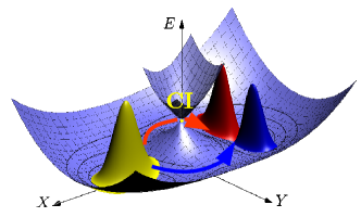
Figure 1: Destructive interference due to geometric phase in low energy dynamics: the initial nuclear density is in yellow and the one at a later time is in red-blue.

Of course, any accurate method of quantum dynamics must reproduce the nodal line appearing in this setup. Mead and TruhlarMead and Truhlar (1979) shown that to capture the GP in simulations using time-independent nuclear basis functions it is necessary to introduce a complex-valued gauge transformation. This transformation requires some global information about the topology of the potential energy surfaces forming CI and thus poses difficulties in application within the on-the-fly framework, where only local information is available. To address this difficulty, we consider two approaches to formulating TDVP using the adiabatic representation and show how the GP can be accounted in each of these approaches.

The total non-relativistic molecular Hamiltonian can be written as

$$\hat{H}(\mathbf{r},\mathbf{R})=\hat{T}_{N}+\hat{H}_{e}(\mathbf{r};\mathbf{R}),$$ (1)

where $\hat{T}_{N}=-\nabla_{\mathbf{R}}^{2}/2$ is the kinetic energy of nuclei, and $\hat{H}_{e}(\mathbf{r};\mathbf{R})$ is the electronic Hamiltonian with electronic $\mathbf{r}$ and nuclear $\mathbf{R}$ coordinates. $\hat{H}_{e}(\mathbf{r};\mathbf{R})$ determines the adiabatic electronic wave-functions $\ket{\phi_{s}(\mathbf{R})}$ and potential energy surfaces $E_{e}^{(s)}(\mathbf{R})$: $\hat{H}_{e}(\mathbf{r};\mathbf{R})\langle\mathbf{r}\ket{\phi_{s}(\mathbf{R})}=E_{e}^{(s)}(\mathbf{R})\langle\mathbf{r}\ket{\phi_{s}(\mathbf{R})}$.

Global adiabatic (GA) representation:

The total non-stationary wave-function can be expanded in the adiabatic representation as

$$\langle\mathbf{r},\mathbf{R}\ket{\Psi(t)}=\sum_{I,s}C_{I}^{(s)}(t)\langle\mathbf{R}\ket{G_{I}^{(s)}}\langle\mathbf{r}\ket{\phi_{s}(\mathbf{R})},$$ (2)

where $C_{I}^{(s)}$ are time dependent coefficients, indices $s$ and $I$ enumerate the electronic and nuclear coherent states (CSs)

$$\langle\mathbf{R}\ket{G_{I}^{(s)}} = \prod_{j=1}^{N}\left(\frac{\omega_{j}}{\pi}\right)^{1/4}\exp\Big{[}-\frac{\omega_{j}}{2}[R_{j}-q_{jI}^{(s)}(t)]^{2}$$ (3)

$$+ip_{jI}^{(s)}[R_{j}-q_{jI}^{(s)}(t)]+\frac{i}{2}p_{jI}^{(s)}q_{jI}^{(s)}\Big{]}$$

with time-dependent positions $\mathbf{q}_{I}^{(s)}=\{q_{jI}^{(s)}\}_{j=1,N}$ and momenta $\mathbf{p}_{I}^{(s)}=\{p_{jI}^{(s)}\}_{j=1,N}$ [$N={\rm dim}(\mathbf{R})$].

Equations of motion (EOM) for positions and momenta of CSs can be obtained using TDVP but resulting EOM would introduce unnecessary complexity for our consideration. Thus, here, we adopt simpler EOM that follow classical dynamics on the adiabatic potential energy surfaces

$$\dot{\mathbf{q}}_{I}^{(s)} = \mathbf{p}_{I}^{(s)}$$ (4)

$$\dot{\mathbf{p}}_{I}^{(s)} = -\frac{E_{e}^{(s)}(\mathbf{R})}{\partial\mathbf{R}}\Big{|}_{\mathbf{R}=\mathbf{q}_{I}^{(s)}}.$$ (5)

This simplifies variation of the total wave-function by restricting it only to the linear coefficients $C_{I}^{(s)}(t)$

$$\delta\langle\mathbf{r},\mathbf{R}\ket{\Psi(t)}=\sum_{I,s}[\delta C_{I}^{(s)}(t)]\langle\mathbf{R}\ket{G_{I}^{(s)}}\langle\mathbf{r}\ket{\phi_{s}(\mathbf{R})}.$$ (6)

Applying the Dirac-Frenkel TDVPDirac (1930); Frenkel (1934)

$$\bra{\delta\Psi}\hat{H}-i\partial_{t}\ket{\Psi}=0$$ (7)

and substituting the $\Psi$ and $\delta\Psi$ expressions from Eqs. (2) and (6) we obtain

$$\sum_{IK,ss^{\prime}}\delta C_{I}^{(s)}\bra{G_{I}^{(s)}}\hat{H}_{N}^{(ss^{\prime})}-i\partial_{t}\ket{G_{K}^{(s^{\prime})}}C_{K}^{(s^{\prime})}=0,$$ (8)

where

$$\hat{H}_{N}^{(ss^{\prime})} = \bra{\phi_{s}(\mathbf{R})}\hat{H}_{e}(\mathbf{R})+\hat{T}_{N}\ket{\phi_{s^{\prime}}(\mathbf{R})}$$ (9)

$$= E_{e}^{(s)}(\mathbf{R})\delta_{ss^{\prime}}+\hat{T}_{N}+\hat{\tau}_{ss^{\prime}},$$ (10)

$$\hat{\tau}_{ss^{\prime}} = -\bra{\phi_{s}(\mathbf{R})}\nabla_{\mathbf{R}}\phi_{s^{\prime}}(\mathbf{R})\rangle\nabla_{\mathbf{R}}$$ (11)

$$-\bra{\phi_{s}(\mathbf{R})}\nabla_{\mathbf{R}}^{2}\phi_{s^{\prime}}(\mathbf{R})\rangle/2.$$

Note that so-called nonadiabatic couplings (NACs) $\hat{\tau}_{ss^{\prime}}$ appear as a result of a global dependence of the electronic wave-functions $\phi_{s}$ on the nuclear coordinates $\mathbf{R}$. Considering independence of $\delta C_{I}^{(s)}$ variations, EOM for the coefficients $C_{I}^{(s)}(t)$ become

$$\sum_{K,s^{\prime}}\bra{G_{I}^{(s)}}\hat{H}_{N}^{(ss^{\prime})}-i\partial_{t}\ket{G_{K}^{(s^{\prime})}}C_{K}^{(s^{\prime})}=0,$$ (12)

Rearranging few terms leads to EOM in the form

$$i\dot{C}_{J}^{(s)} = \sum_{I,K}\bra{G_{J}^{(s)}}G_{I}^{(s)}\rangle^{-1}\Big{[}\bra{G_{I}^{(s)}}\hat{H}_{N}^{(ss^{\prime})}\ket{G_{K}^{(s^{\prime})}}$$ (13)

$$-i\bra{G_{I}^{(s)}}\partial_{t}G_{K}^{(s^{\prime})}\rangle\Big{]}C_{K}^{(s^{\prime})}.$$

where $\bra{G_{J}^{(s)}}G_{I}^{(s)}\rangle^{-1}$ are elements of the inverse CS overlap matrix. Time-derivatives of CSs needed in Eq. (13) are derived using the chain rule

$$\ket{\partial_{t}G_{K}^{(s^{\prime})}} = \ket{\frac{\partial G_{K}^{(s^{\prime})}}{\partial\mathbf{q}_{K}^{(s^{\prime})}}}\dot{\mathbf{q}}_{K}^{(s^{\prime})}(t)+\ket{\frac{\partial G_{K}^{(s^{\prime})}}{\partial\mathbf{p}_{K}^{(s^{\prime})}}}\dot{\mathbf{p}}_{K}^{(s^{\prime})}(t).$$ (14)

The difficulty associated with a proper treatment of the nuclear dynamics using global adiabatic electronic functions is that $\ket{\phi_{s}(\mathbf{R})}$ are double-valued functions with respect to $\mathbf{R}$ in the CI case. To have a single-valued total wave-function in Eq. (2) the nuclear wave-function must also be double-valued, which is not the case for typical Gaussian-like basis sets [Eq. (3)]. In order to include GP related effects in the nuclear dynamics one needs to substitute the real but double-valued adiabatic electronic wave-functions $\ket{\phi_{s}(\mathbf{R})}$ by their complex but single-valued counterparts: $\ket{\tilde{\phi}_{s}(\mathbf{R})}=e^{i\theta_{s}(\mathbf{R})}\ket{\phi_{s}(\mathbf{R})}$, where $e^{i\theta_{s}(\mathbf{R})}$ is a phase factor that changes its sign when $\mathbf{R}$ follows any curve encircling the CI. This phase factor can be seen as a gauge transformation which is needed when a single-valued basis functions for the nuclear counterpart are used.

Moving crude adiabatic (MCA) representation:

Alternatively, EOM can be derived using a different ansatz for the total wave-function

$$\langle\mathbf{r},\mathbf{R}\ket{\Psi(t)}=\sum_{I,s}C_{I}^{(s)}(t)\langle\mathbf{R}\ket{G_{I}^{(s)}}\langle\mathbf{r}\ket{\phi_{s}(\mathbf{q}_{I}^{(s)})},$$ (15)

here the electronic functions are evaluated only at the centres of CSs, $\mathbf{q}_{I}^{(s)}$, and thus do not depend on the nuclear coordinates $\mathbf{R}$. To simplify the notation we will denote $\ket{\phi_{s}(\mathbf{q}_{I}^{(s)})}$ as $\ket{\phi_{I}^{(s)}}$. Treating CS motion classically [Eqs. (4) and (5)] we repeat the derivation of EOM for $C_{I}^{(s)}(t)$ in Eq. (15) and obtain

$$i\dot{C}_{J}^{(s^{\prime\prime})} = \sum_{I,K}\bra{G_{J}^{(s^{\prime\prime})}\phi_{J}^{(s^{\prime\prime})}}G_{I}^{(s)}\phi_{I}^{(s)}\rangle^{-1}\Big{[}\bra{G_{I}^{(s)}}\hat{H}_{IK}^{(ss^{\prime})}\ket{G_{K}^{(s^{\prime})}}$$ (16)

$$-i\bra{\phi_{I}^{(s)}G_{I}^{(s)}}\phi_{K}^{(s^{\prime})}\partial_{t}G_{K}^{(s^{\prime})}\rangle\Big{]}C_{K}^{(s^{\prime})},$$

where $\bra{G_{J}^{(s^{\prime\prime})}\phi_{J}^{(s^{\prime\prime})}}G_{I}^{(s)}\phi_{I}^{(s)}\rangle^{-1}$ are elements of the total inverse overlap matrix, and

$$\hat{H}_{IK}^{(ss^{\prime})} = \bra{\phi_{I}^{(s)}}\hat{H}_{e}(\mathbf{R})\ket{\phi_{K}^{(s^{\prime})}}+\bra{\phi_{I}^{(s)}}\phi_{K}^{(s^{\prime})}\rangle\hat{T}_{N}$$

$$-i\bra{\phi_{I}^{(s)}}\partial_{t}\phi_{K}^{(s^{\prime})}\rangle.$$

Here, the adiabatic electronic functions obtained at different points of nuclear geometry and corresponding to different electronic states are non-orthogonal: $\bra{\phi_{I}^{(s)}}\phi_{K}^{(s^{\prime})}\rangle\neq\delta_{ss^{\prime}}$ if $I\neq K$. Also, the electronic functions are not eigenfunctions of the electronic Hamiltonian for all values of $\mathbf{R}$, therefore, $\bra{\phi_{I}^{(s)}}\hat{H}_{e}(\mathbf{R})\ket{\phi_{K}^{(s^{\prime})}}$ is a $\mathbf{R}$ and $t$ dependent matrix of functions

Using the chain rule, the electronic time-derivative couplings in Eq. (Moving crude adiabatic (MCA) representation:) can be expressed as

$$\bra{\phi_{I}^{(s)}}\partial_{t}\phi_{K}^{(s^{\prime})}\rangle = \bra{\phi_{I}^{(s)}}\frac{\partial\phi_{K}^{(s^{\prime})}}{\partial\mathbf{q}_{K}^{(s^{\prime})}}\rangle\dot{\mathbf{q}}_{K}^{(s^{\prime})}.$$ (18)

Considering the equivalence between dependencies of the MCA electronic functions on centres of CSs and the GA electronic functions on $\mathbf{R}$, the electronic function derivatives in Eq. (18) are similar to the first order derivative part of NACs in Eq. (11). The first order derivative couplings diverge at the point of the CI, however, since the CS centres form a measure zero subset, CSs will never have their centres exactly at the CI seam. Note that in the MCA representation there are no analogues of the second order derivative parts of NACs. The second order derivatives in NACs pose difficulties for integrating EOM due to their $1/R^{2}$ divergent behavior with the distance from the CI $R$.Meek and Levine (2016a)

From the GP point of view, the MCA formalism can be thought as a truly diabatic formalism since the electronic functions do not have the dependence on $\mathbf{R}$, and thus problems emerging in the GA representation do not appear here. Nevertheless, due to a parametric dependence of the adiabatic electronic functions on CSs’ centres, the MCA representation has GPs carried by the electronic functions.

We illustrate nuclear dynamics in the introduced representations for a 2D-LVC model where formulated EOM can be simulated without additional approximations and where the GP plays a significant role. The total Hamiltonian for 2D-LVC is

$$\hat{H}_{\rm LVC}=\begin{pmatrix}\hat{T}_{N}+V_{11}&V_{12}\\ V_{12}&\hat{T}_{N}+V_{22}\end{pmatrix},$$ (19)

where $\hat{T}_{N}=-\frac{1}{2}(\partial^{2}/\partial x^{2}+\partial^{2}/\partial y^{2})$ is the nuclear kinetic energy operator, $V_{11}$ and $V_{22}$ are the diabatic potentials represented by identical 2D parabolas shifted in the $x$-direction by $a$

$$V_{11}(\mathbf{R})={} \frac{\omega^{2}}{2}\left[(x+a)^{2}+y^{2}\right],$$ (20)

$$V_{22}(\mathbf{R})={} \frac{\omega^{2}}{2}\left[(x-a)^{2}+y^{2}\right].$$ (21)

To have the CI in the adiabatic representation, $V_{11}$ and $V_{22}$ are coupled by a linear potential $V_{12}(\mathbf{R})=cy$. Thus for this example we have $\mathbf{R}=(x,y)$ and the electronic Hamiltonian can be defined as $\hat{H}_{e}(\mathbf{R})=\sum_{ij}\ket{\varphi_{i}}V_{ij}(\mathbf{R})\bra{\varphi_{j}}$, where $\ket{\varphi_{i}}$’s are the diabatic electronic states.

Switching to the adiabatic representation is done by rotating the electronic basis into the adiabatic states

$$\ket{\phi_{1}(\mathbf{R})} = \phantom{-}\cos\theta(\mathbf{R})\,\ket{\varphi_{1}}+\sin\theta(\mathbf{R})\,\ket{\varphi_{2}},$$ (22)

$$\ket{\phi_{2}(\mathbf{R})} = -\sin\theta(\mathbf{R})\,\ket{\varphi_{1}}+\cos\theta(\mathbf{R})\,\ket{\varphi_{2}},$$ (23)

which diagonalize the potential matrix. $\theta(\mathbf{R})$ is a rotation angle

$$\theta=\frac{1}{2}\arctan\dfrac{2\,V_{12}}{V_{22}-V_{11}}.$$ (24)

If we track $\theta$ changes continuously along a contour encircling the CI, it will change by $\pi$, which flips the sign of the phase factor $e^{i\theta}$.Izmaylov, Li, and Joubert-Doriol (2016) The nuclear 2D-LVC Hamiltonian in the adiabatic representation is

$$\hat{H}_{\text{adi}}=\begin{pmatrix}\hat{T}_{N}+\hat{\tau}_{11}&\hat{\tau}_{12}\\ \hat{\tau}_{21}&\hat{T}_{N}+\hat{\tau}_{22}\end{pmatrix}+\begin{pmatrix}E_{e}^{(-)}&0\\ 0&E_{e}^{(+)}\end{pmatrix},$$ (25)

where

$$E_{e}^{(\pm)}= {}\dfrac{1}{2}\left(V_{11}+V_{22}\right)\pm\dfrac{1}{2}\sqrt{\left(V_{11}-V_{22}\right)^{2}+4V_{12}^{2}}$$ (26)

are the adiabatic energy surfaces and

$$\hat{\tau}_{11} {}=\hat{\tau}_{22}=\frac{1}{2}\nabla\theta\cdot\nabla\theta$$ (27)

$$\hat{\tau}_{12} {}=-\hat{\tau}_{21}=\frac{1}{2}\left(\nabla^{2}\theta+2\nabla\theta\cdot\nabla\right)$$ (28)

are NACs.

In order to include the GP we use the gauge transformation of the electronic functions that can be seen as a modification of the nuclear Hamiltonian $H_{\text{adi}}^{\rm GP}=e^{-i\theta}\hat{H}_{\rm adi}e^{i\theta}$.Ryabinkin, Joubert-Doriol, and Izmaylov (2014) This transformation leads to modification of NACs

$$H_{\text{adi}}^{\rm GP}=\begin{pmatrix}\hat{T}_{N}+\hat{\tau}_{11}^{\rm GP}&\hat{\tau}_{12}^{\rm GP}\\ \hat{\tau}_{21}^{\rm GP}&\hat{T}_{N}+\hat{\tau}_{22}^{\rm GP}\end{pmatrix}+\begin{pmatrix}E_{e}^{(-)}&0\\ 0&E_{e}^{(+)}\end{pmatrix},$$ (29)

where

$$\hat{\tau}_{11}^{\rm GP}=\hat{\tau}_{22}^{\rm GP} = (\nabla\theta)^{2}-\frac{i}{2}(\nabla^{2}\theta+2\nabla\theta\nabla),$$ (30)

$$\hat{\tau}_{12}^{\rm GP}=-\hat{\tau}_{21}^{\rm GP} = -i(\nabla\theta)^{2}+\frac{1}{2}(\nabla^{2}\theta+2\nabla\theta\nabla).$$ (31)

For the MCA representation, the electronic states are calculated as

$$\ket{\phi_{I}^{(1)}} = \phantom{-}\cos\theta(\mathbf{q}_{I}^{(1)})\,\ket{\varphi_{1}}+\sin\theta(\mathbf{q}_{I}^{(1)})\,\ket{\varphi_{2}},$$ (32)

$$\ket{\phi_{I}^{(2)}} = -\sin\theta(\mathbf{q}_{I}^{(2)})\,\ket{\varphi_{1}}+\cos\theta(\mathbf{q}_{I}^{(2)})\,\ket{\varphi_{2}},$$ (33)

where $q_{I}^{(1)}$ and $q_{I}^{(2)}$ are centres of corresponding CSs. Therefore, integrals $\bra{\phi_{I}^{(s)}}H_{e}(\mathbf{R})\ket{\phi_{J}^{(s)}}$ for the 2D-LVC model are simply linear combinations of $V_{kl}(\mathbf{R})$ multiplied by $\cos$ and $\sin$ functions.

To illustrate the performance of all three approaches in reproducing the GP we simulate nuclear dynamics of the initial wave-function

$$\langle\mathbf{R}\ket{\Psi(t=0)}=\frac{\ket{\phi_{1}}}{\sqrt{2}}[\langle\mathbf{R}\ket{g_{1}^{(1)}}+\langle\mathbf{R}\ket{g_{2}^{(1)}}]$$ (34)

that is comprised of two CSs, $\ket{G_{I}^{(1)}}=\ket{G_{I}^{(1)}(q,p_{I})}$ centred at the same point $q=(-1.5,0)$ of the ground potential energy surface, but with momenta $p_{1}=(0.1,0.5)$ and $p_{2}=(0.1,-0.5)$, which have the opposite $y$-components. Using three different Hamiltonians, Eqs. (Moving crude adiabatic (MCA) representation:), (25), and (29), we simulate time-dependent wave-functions and monitor the total nuclear density $\rho_{n}(\mathbf{R},t)={\rm Tr}_{e}[\langle\mathbf{R}\ket{\Psi(t)}\bra{\Psi(t)}\mathbf{R}\rangle]$, where ${\rm Tr}_{e}$ is the trace over the electronic coordinates. Figure 2 illustrates that dynamics with the adiabatic Hamiltonian (25) misses the GP, while two other Hamiltonians reproduce the GP induced destructive interference perfectly. However, mechanisms for the destructive interference in the two approaches is quite different: For the GA representation, two CSs acquire different phases from the $-i\nabla\theta\nabla$ part of the diagonal NAC [Eq. (30)] because the $\theta$ angle is proportional to the geometric angle between the initial and final positions of a CS with respect to the CI. In the MCA representation, CSs acquire different phases due to GPs of the associated electronic wave-functions.

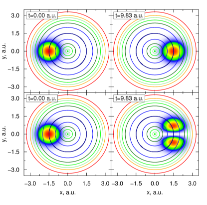
Figure 2: Nuclear probability densities for the approach ignoring GP (top) and including GP (bottom): the initial density distributions are on the left panels, density distributions at a later time on the right panels. Contours of the ground adiabatic state potential from $H_{\rm LVC}$ ($\omega=2$, $a=1.5$, $c=6$) are superimposed on the density distributions.

In conclusion, we illustrated that GP effects can be successfully captured using both global and moving crude adiabatic representations. However, capturing the GP in the GA representation seems difficult for calculations beyond models. The systematic application of TDVP with the GA electronic functions becomes especially difficult for the on-the-fly calculations, not only because of the necessity to generate the gauge transformation $e^{i\theta(\mathbf{R})}$ using only local information but also because of the second order derivative NACs whose integrals with Gaussians are divergent.Meek and Levine (2016a) On both accounts, employing the MCA representation is much more practical: GPs are always carried by the electronic functions and numerically difficult second order derivative NACs never appear in the formalism. Interestingly, in previous works on ab initio multiple spawning (AIMS), Martinez, Ben-Nun, and Levine (1996); Ben-Nun and Martinez (1998); Ben-Nun, Quenneville, and Martinez (2000); Yang et al. (2009); Ben-Nun and Martinez (2002) the derivation was presented starting with the GA representation but the actual working EOM for the linear coefficients were very similar to the ones obtained in the current work using the MCA representation. This was the result of approximations needed to make AIMS EOM feasible for simulating dynamics in realistic systems. The current work provides a rigorous framework of the MCA representation that justifies some of the approximations made in AIMS. Also, the MCA representation can be seen as an effortless realization of a recently proposed on-the-fly diabatization to solve the problem of numerical difficulties in integration of the second order NACs.Meek and Levine (2016b)

Acknowledgments: Authors are grateful to Todd Martinez, Benjamin Levine, and Michael Schuurman for stimulating discussions. A.F.I. acknowledges funding from a Sloan Research Fellowship and the Natural Sciences and Engineering Research Council of Canada (NSERC) through the Discovery Grants Program.

References

- Kramer and Saraceno (1981) P. Kramer and M. Saraceno, Geometry of the Time-Dependent Variational Principle in Quantum Mechanics (Springer, New York, 1981).
- Dirac (1930) P. A. M. Dirac, Proc. Cambridge Philos. Soc. 26, 376 (1930).
- Frenkel (1934) J. Frenkel, Wave Mechanics (Clarendon Press, Oxford, 1934).
- Meyer, Manthe, and Cederbaum (1990) H.-D. Meyer, U. Manthe, and L. S. Cederbaum, Chem. Phys. Lett. 165, 73 (1990).
- Wang and Thoss (2003) H. Wang and M. Thoss, J. Chem. Phys. 119, 1289 (2003).
- (6) G. A. Worth, M. H. Beck, A. Jackle and H.-D. Meyer, The MCTDH Package, Development Version 9.0, University of Heidelberg, Heidelberg, Germany, 2009.
- Yang et al. (2009) S. Yang, J. D. Coe, B. Kaduk, and T. J. Martínez, The Journal of Chemical Physics 130, 134113 (2009).
- Ben-Nun and Martinez (2002) M. Ben-Nun and T. J. Martinez, Advances in Chemical Physics 121, 439 (2002).
- Shalashilin (2009) D. V. Shalashilin, The Journal of Chemical Physics 130, 244101 (2009).
- Burghardt, Giri, and Worth (2008) I. Burghardt, K. Giri, and G. A. Worth, The Journal of Chemical Physics 129, 174104 (2008).
- Worth, Robb, and Lasorne (2008) G. A. Worth, M. A. Robb, and B. Lasorne, Molecular Physics 106, 2077 (2008).
- Worth, Robb, and Burghardt (2004) G. A. Worth, M. A. Robb, and I. Burghardt, Faraday Discuss. 127, 307 (2004).
- Izmaylov (2013) A. F. Izmaylov, The Journal of Chemical Physics 138, 104115 (2013).
- Saita and Shalashilin (2012) K. Saita and D. V. Shalashilin, The Journal of Chemical Physics 137, 22A506 (2012).
- Domcke and Yarkony (2012) W. Domcke and D. R. Yarkony, Annu. Rev. Phys. Chem. 63, 325 (2012).
- Yarkony (1996) D. R. Yarkony, Rev. Mod. Phys. 68, 985 (1996).
- Yarkony (1998) D. R. Yarkony, Acc. Chem. Res. 31, 511 (1998).
- Yarkony (2001) D. R. Yarkony, J. Phys. Chem. A 105, 6277 (2001).
- Longuet-Higgins et al. (1958) H. C. Longuet-Higgins, U. Opik, M. H. L. Pryce, and R. A. Sack, Proc. R. Soc. A 244, 1 (1958).
- Mead and Truhlar (1979) C. A. Mead and D. G. Truhlar, J. Chem. Phys. 70, 2284 (1979).
- Berry (1984) M. V. Berry, Proc. R. Soc. A 392, 45 (1984).
- Mead (1992) C. A. Mead, Rev. Mod. Phys. 64, 51 (1992).
- Wittig (2012) C. Wittig, Phys. Chem. Chem. Phys. 14, 6409 (2012).
- Althorpe (2006) S. C. Althorpe, J. Chem. Phys. 124, 084105 (2006).
- Kendrick (2003) B. K. Kendrick, J. Phys. Chem. A 107, 6739 (2003).
- Ryabinkin and Izmaylov (2013) I. G. Ryabinkin and A. F. Izmaylov, Phys. Rev. Lett. 111, 220406 (2013).
- Joubert-Doriol, Ryabinkin, and Izmaylov (2013) L. Joubert-Doriol, I. G. Ryabinkin, and A. F. Izmaylov, J. Chem. Phys. 139, 234103 (2013).
- Ryabinkin, Joubert-Doriol, and Izmaylov (2014) I. G. Ryabinkin, L. Joubert-Doriol, and A. F. Izmaylov, J. Chem. Phys. 140, 214116 (2014).
- Xie et al. (2016) C. Xie, J. Ma, X. Zhu, D. R. Yarkony, D. Xie, and H. Guo, Journal of the American Chemical Society 138, 7828 (2016).
- Hazra, Balakrishnan, and Kendrick (2015) J. Hazra, N. Balakrishnan, and B. K. Kendrick, Nature Communications 6, 1 (2015).
- Min et al. (2014) S. K. Min, A. Abedi, K. S. Kim, and E. K. U. Gross, Phys. Rev. Lett. 113, 263004 (2014).
- Requist, Tandetzky, and Gross (2016) R. Requist, F. Tandetzky, and E. K. U. Gross, Phys. Rev. A 93, 042108 (2016).
- Schön and Köppel (1995) J. Schön and H. Köppel, J. Chem. Phys. 103, 9292 (1995).
- Note (1) For simplicity, we use the nuclear coordinates in the mass-weighted form, and atomic units are used throughout this paper.
- Meek and Levine (2016a) G. A. Meek and B. G. Levine, The Journal of Chemical Physics 144, 184109 (2016a).
- Izmaylov, Li, and Joubert-Doriol (2016) A. F. Izmaylov, J. Li, and L. Joubert-Doriol, Journal of Chemical Theory and Computation 12, 5278 (2016).
- Martinez, Ben-Nun, and Levine (1996) T. J. Martinez, M. Ben-Nun, and R. D. Levine, The Journal of Physical Chemistry 100, 7884 (1996).
- Ben-Nun and Martinez (1998) M. Ben-Nun and T. J. Martinez, The Journal of Chemical Physics 108, 7244 (1998).
- Ben-Nun, Quenneville, and Martinez (2000) M. Ben-Nun, J. Quenneville, and T. Martinez, J. Phys. Chem. A 104, 5161 (2000).
- Meek and Levine (2016b) G. A. Meek and B. G. Levine, The Journal of Chemical Physics 145, 184103 (2016b).