Spin-chain model for strongly interacting one-dimensional Bose-Fermi mixtures

Abstract

Strongly interacting one-dimensional (1D) Bose-Fermi mixtures form a tunable XXZ spin chain. Within the spin-chain model developed here, all properties of these systems can be calculated from states representing the ordering of the bosons and fermions within the atom chain and from the ground-state wave function of spinless noninteracting fermions. We validate the model by means of an exact diagonalization of the full few-body Hamiltonian in the strongly interacting regime. Using the model, we explore the phase diagram of the atom chain as a function of the boson-boson (BB) and boson-fermion (BF) interaction strengths and calculate the densities, momentum distributions, and trap-level occupancies for up to 17 particles. In particular, we find antiferromagnetic (AFM) and ferromagnetic (FM) order and a demixing of the bosons and fermions in certain interaction regimes. We find, however, no demixing for equally strong BB and BF interactions in agreement with earlier calculations that combined the Bethe ansatz with a local-density approximation.

I Introduction

Ultracold atoms are ideally suited to study strongly correlated one-dimensional (1D) systems due to their high degree of control and tunability Cazalilla11 ; Guan13 . These advantageous features have led to the observation of the Tonks-Girardeau gas Kinoshita04 ; Paredes04 , the controlled preparation of a highly excited super-Tonks gas Haller09 ; Astrakharchik05 , undamped dynamics in strongly interacting 1D Bose gases Kinoshita06 , and the deterministic preparation of 1D few-fermion systems with tunable interactions Serwane11 ; Zuern12 ; Zuern13 ; Wenz13 ; Murmann15 . Moreover, it became possible to realize a variety of artificial 1D systems consisting, e.g., of atoms with a large spin Pagano14 or Bose-Fermi mixtures with mixed statistics Schreck01 .

These developments have renewed the interest in Girardeau’s Bose-Fermi mapping for 1D spinless bosons with infinite $\delta$ repulsion Girardeau60 leading to generalizations for Bose-Fermi mixtures Girardeau07 , spin-1 bosons Deuretzbacher08 , and spin-1/2 fermions Guan09 . Only recently it was found that these exact solutions are also useful for the perturbative treatment of strongly interacting 1D systems Volosniev14 . Different from one-component systems, the ground state of multicomponent systems with infinite $\delta$ repulsion is highly degenerate Girardeau07 ; Deuretzbacher08 ; Guan09 . This is due to the fact that strongly interacting 1D particles localize and arrange themselves in a spin chain Deuretzbacher08 ; Matveev08 ; Deuretzbacher14 . This offers the exciting possibility to study quantum magnetism without the need for an optical lattice Deuretzbacher14 ; Volosniev15 ; Yang15 ; Massignan15 ; Yang16a .

Theoretical studies of Bose-Fermi mixtures in optical lattices predicted composite fermions consisting of one fermion and one ore more bosons, or, respectively, bosonic holes Lewenstein04 and polarons Mathey07 . In addition, pairing, collapse, and demixing can occur in homogeneous 1D systems of strongly interacting bosons and fermions Cazalilla03 . For equally strong boson-boson (BB) and boson-fermion (BF) $\delta$ interactions, the model can be solved exactly via the Bethe ansatz Imambekov06 ; Guan08 . Selected states of the degenerate ground-state multiplet have been constructed in the Tonks-Girardeau regime of infinite $\delta$ repulsion Girardeau07 and classified using Young’s tableaux Fang11 . Recently, all states of the multiplet have been constructed for few (up to 6) particles Hu16a ; Dehkharghani17 ; Zinner15 and strongly interacting mixtures with additional weak $p$-wave interactions have been studied Hu16b ; Yang16b .

Here, we develop a spin-chain model for 1D Bose-Fermi mixtures with nearly infinite $\delta$ interactions AncillaryFiles . We check the validity of the model by diagonalizing the full few-body Hamiltonian numerically in the strongly interacting regime. Using the spin-chain model, we then calculate the ground-state densities, momentum distributions, and occupancies of the harmonic-trap levels for atom chains consisting of up to 17 particles. Moreover, we determine the ground-state phases of these atom chains, finding antiferromagnetic (AFM) and ferromagnetic (FM) order and a demixing of the bosons and fermions for particular values of the BB and BF interaction strengths. However, no demixing is found for equally strong BB and BF interactions although the bosons are predominantly in the trap center and the fermions are predominantly at the edges of the trap Imambekov06 .

II Spin-chain model

We consider a 1D mixture of $N_{B}$ bosons and $N_{F}$ fermions (total particle number $N=N_{B}+N_{F}$). Both species are assumed to have the same masses, $M_{B}=M_{F}=M$, and experience the same trapping potential $V(z)$. The bosons interact with each other through a $\delta$ potential of strength $g_{BB}$ and with the fermions through a $\delta$ potential of strength $g_{BF}$. The many-body Hamiltonian of the system is given by

$$H \!\!= \!\!\sum_{i=1}^{N}\left[-\frac{\hbar^{2}}{2M}\frac{\partial^{2}}{\partial z_{i}^{2}}+V(z_{i})\right]\!+g_{BB}\!\sum_{i=1}^{N_{B}-1}\!\sum_{j=i+1}^{N_{B}}\!\delta(z_{i}-z_{j})$$ (1)

$$\!\!+\;g_{BF}\sum_{i=1}^{N_{B}}\sum_{j=N_{B}+1}^{N}\delta(z_{i}-z_{j}).$$

The interaction strengths $g_{BB}$ and $g_{BF}$ are freely tunable through a magnetic Feshbach resonance Inouye98 and through the strong radial confinement Olshanii98 .

Here, we focus on the strongly interacting regime, where the absolute value of both interaction strengths is large, i. e., $|g_{BB}|\approx\infty$ and $|g_{BF}|\approx\infty$. Furthermore, we consider only the highly excited super-Tonks states Haller09 ; Astrakharchik05 ; Zuern12 if at least one of the interaction strengths is attractive. Under these conditions, the atoms order in a row and form a spin chain Deuretzbacher08 ; Matveev08 ; Deuretzbacher14 ; Comment1 . An arbitrary state of the spin chain is given by

$$|\chi\rangle=\sum_{m_{1},\dotsc,m_{N}}c_{m_{1},\dotsc,m_{N}}|m_{1},\dotsc,m_{N}\rangle,$$ (2)

where each basis state $|m_{1},\dotsc,m_{N}\rangle$ with $m_{i}=B,F$ corresponds to a particular ordering of the bosons ($B$) and fermions ($F$) and can be constructed from the wave function of $N$ spinless noninteracting fermions Fang11 (see Appendix A).

Nearest neighboring particles of the spin chain interact with each other through the effective Hamiltonian Hu16b

$$\!\!\!H_{\mathrm{eff}} \!= \!E_{F}\openone-2\sum_{i=1}^{N-1}J_{i}^{(BB)}|B\rangle_{i}|B\rangle_{i+1}\langle B|_{i}\langle B|_{i+1}$$ (3)

$$\!-\sum_{i=1}^{N-1}J_{i}^{(BF)}\Bigl{(}|B\rangle_{i}|F\rangle_{i+1}+|F\rangle_{i}|B\rangle_{i+1}\Bigr{)}$$

$$\!\times\Bigl{(}\langle B|_{i}\langle F|_{i+1}+\langle F|_{i}\langle B|_{i+1}\Bigr{)},$$

as shown in Appendix B. Here, $E_{F}$ is the ground-state energy of $N$ spinless noninteracting fermions in the trapping potential $V(z)$ and $J_{i}^{(BB)}$ and $J_{i}^{(BF)}$ are the exchange coefficients of nearest neighbor bosons or bosons and fermions, respectively. The exchange coefficients are given by $J_{i}^{(BB)}=C_{i}/g_{BB}$ and $J_{i}^{(BF)}=C_{i}/g_{BF}$ with Volosniev14 ; Deuretzbacher14

$$C_{i}=\frac{N!\hbar^{4}}{M^{2}}\!\int\!dz_{1}\dotsi dz_{N}\delta(z_{i}-z_{i+1})\theta(z_{1},\dotsc,z_{N})\!\left|\frac{\partial\psi_{F}}{\partial z_{i}}\right|^{2}\!\!,$$ (4)

where $\theta(z_{1},\dotsc,z_{N})=1$ if $z_{1}<\dotsb<z_{N}$, and zero otherwise, and where $\psi_{F}$ is the ground-state wave function of $N$ spinless noninteracting fermions in the trap $V(z)$. The $C_{i}$ can be efficiently calculated for large $N$ Deuretzbacher16 ; Loft16 ; Yang16c .

By identifying bosons and fermions with pseudospin-up and -down particles, respectively, Eq. (3) can be rewritten in terms of the Pauli matrices $\sigma_{x}^{(i)}$, $\sigma_{y}^{(i)}$, and $\sigma_{z}^{(i)}$:

$$\mspace{-20.0mu}H_{\mathrm{eff}}=-\frac{1}{2}\sum_{i=1}^{N-1}\biggl{\{}J_{i}^{(BF)}\left[\sigma_{x}^{(i)}\sigma_{x}^{(i+1)}+\sigma_{y}^{(i)}\sigma_{y}^{(i+1)}\right]$$

$$\mspace{-20.0mu}+\left[J_{i}^{(BB)}-J_{i}^{(BF)}\right]\sigma_{z}^{(i)}\sigma_{z}^{(i+1)}+J_{i}^{(BB)}\left[\sigma_{z}^{(i)}+\sigma_{z}^{(i+1)}\right]\biggr{\}}.$$

Here, we neglected the diagonal matrix

$$\left\{E_{F}-\frac{1}{2}\sum_{i=1}^{N-1}\left[J_{i}^{(BB)}+J_{i}^{(BF)}\right]\right\}\openone.$$ (6)

Equation (II) is the Hamiltonian of an XXZ spin chain in an inhomogeneous magnetic field along the $z$ axis. Similar effective Hamiltonians have been derived for strongly interacting Bose-Bose mixtures Volosniev15 ; Massignan15 ; Yang16a and strongly interacting mixtures with weak $p$-wave interactions Hu16b ; Yang16b .

The densities of the bosons (${m=B}$) and fermions (${m=F}$) are given by Deuretzbacher08

$$\rho_{m}(z)=\sum_{i=1}^{N}\rho^{(i)}(z)\rho_{m}^{(i)}$$ (7)

with the probability to find the $i$th particle at position $z$,

$$\rho^{(i)}(z)=N!\int dz_{1}\dotsi dz_{N}\delta(z-z_{i})\theta(z_{1},\dotsc,z_{N})|\psi_{F}|^{2},$$ (8)

and the probability that the $i$th particle is a boson ($m=B$) or fermion ($m=F$),

$$\rho_{m}^{(i)}=\!\sum_{m_{1},\dotsc,m_{N}}\bigl{|}\langle m_{1},\dotsc,m_{N}|\chi\rangle\bigr{|}^{2}\delta_{m,m_{i}}.$$ (9)

The one-body density matrix of the bosons ($m=B$) and fermions ($m=F$) is given by

$$\rho_{m}(z,z^{\prime})=\sum_{i,j=1}^{N}\rho^{(i,j)}(z,z^{\prime})\rho_{m}^{(i,j)}$$ (10)

with Yang15 ; Deuretzbacher16

$$\mspace{-20.0mu}\rho^{(i,j)}(z,z^{\prime})=N!\int dz_{1}\dotsi dz_{i-1}dz_{i+1}\dotsi dz_{N}$$

$$\times\Bigl{[}\theta(z_{1},\dotsc,z_{N})\bigl{|}\psi_{F}(z_{1},\dotsc,z_{N})\bigr{|}\Bigr{]}_{z_{i}=z}$$

$$\times\Bigl{[}\theta(z_{P_{i,\dotsc,j}(1)},\dotsc,z_{P_{i,\dotsc,j}(N)})\bigl{|}\psi_{F}(z_{1},\dotsc,z_{N})\bigr{|}\Bigr{]}_{z_{i}=z^{\prime}}$$

and

$$\rho^{(i,j)}_{m}=\langle\chi|m\rangle_{i}\langle m|_{i}\hat{P}_{i,\dotsc,j}^{(BF)}|\chi\rangle,$$ (12)

as shown in Appendix C. Here, we defined $\hat{P}_{i,\dotsc,j}^{(BF)}=(-1)^{N_{\mathrm{tr}}}\hat{P}_{i,\dotsc,j}$ with the loop permutation operator $\hat{P}_{i,\dotsc,j}$, which moves a particle from position $j$ to position $i$ (see Appendix A for details). $N_{\mathrm{tr}}$ is the number of transpositions of neighboring fermions when $\hat{P}_{i,\dotsc,j}$ acts on $|m_{1},\dotsc,m_{N}\rangle$. The momentum distributions and occupancies of the trap levels are related to the one-body density matrices by

$$\rho_{m}(k)=\frac{1}{2\pi}\int dzdz^{\prime}e^{\mathbbm{i}k(z-z^{\prime})}\rho_{m}(z,z^{\prime})$$ (13)

and

$$\rho_{m}(n)=\int dzdz^{\prime}\phi_{n}(z)\phi_{n}^{*}(z^{\prime})\rho_{m}(z,z^{\prime})$$ (14)

with the eigenfunctions $\phi_{n}(z)$ of the trap $V(z)$.

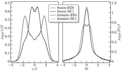
Figure 1: Comparison of the ground-state densities (left) and momentum distributions (right) of a mixture of two bosons and two fermions (2B2F mixture) in a harmonic trap calculated by means of an exact diagonalization (ED) of the full few-body Hamiltonian (solid lines) and from the spin-chain (SC) model (dashed lines) for equal BB and BF interaction strengths ($g_{BB}=g_{BF}=15\hbar\omega l$). $\omega$ and $l$ are the frequency and length scale of the harmonic oscillator.

We have tested the validity of the spin-chain model by comparing its results to those of an exact diagonalization of the full few-body Hamiltonian (1) for up to four particles in a harmonic trap. Both approaches should lead to the same results in the Tonks-Girardeau regime, $g_{BB}=g_{BF}>10\hbar\omega l$ Deuretzbacher07 ; Deuretzbacher14 $\bigl{[}\omega$ is the frequency and $l=\sqrt{\hbar/(m\omega)}$ is the length scale of the harmonic oscillator$\bigr{]}$. Indeed, the comparison showed excellent agreement for the spectrum, the densities, and the momentum distributions for mixtures consisting of one boson and three fermions (1B3F mixture), two bosons and two fermions (2B2F mixture), and three bosons and one fermion (3B1F mixture). As an example, we show in Fig. 1 the result of such a comparison for the ground-state densities and momentum distributions of a 2B2F mixture for equally strong BB and BF interactions, $g_{BB}=g_{BF}=15\hbar\omega l$. These ground-state densities agree with Refs. Hu16a ; Dehkharghani17 .

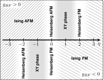
Figure 2: Phase diagram of the Bose-Fermi chain as a function of $\eta=|g_{BF}|/g_{BB}$ for $g_{BF}>0$ (upper part) and $g_{BF}<0$ (lower part).

III Phases and densities

The ground-state phases of the effective Hamiltonian (3) or, respectively, (II) are determined by the interplay of the BB and BF interactions. In particular, we distinguish five different phases, as shown in the phase diagram in Fig. 2, which follow from the phases of the homogeneous XXZ chain in the absence of an external magnetic field Mikeska04 . For dominant BB exchange couplings, which corresponds to the parameter regime $|\eta|=|J_{i}^{(BB)}/J_{i}^{(BF)}|\gg 1$, the spin chain is in the Ising AFM ($J_{i}^{(BB)}<0$) or FM ($J_{i}^{(BB)}>0$) state. For $J_{i}^{(BB)}\approx J_{i}^{(BF)}$ (gray shaded regions around $\eta=\pm 1$), the spin chain is in the XY phase. These phases are characterized by strong FM ($J_{i}^{(BF)}>0$) or AFM ($J_{i}^{(BF)}<0$) $xy$ correlations. At the edges of the XY phases ($\eta=0,\pm 2$) the system is in the Heisenberg AFM or FM phases. Note that we consider the highly excited (metastable) super-Tonks states Haller09 ; Astrakharchik05 in the regime of attractive interactions and, therefore, do not obtain collapse and pairing Cazalilla03 .

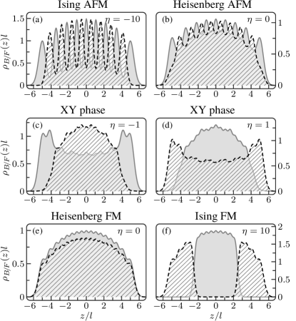
Figure 3: Ground-state densities of a harmonically trapped Bose-Fermi mixture consisting of nine bosons (solid) and eight fermions (dashed) for $g_{BF}<0$ (left) and $g_{BF}>0$ (right). The different phases are described in the text. $l$ is the harmonic oscillator length.

Ising FM and AFM order $(|\eta|\gg 1)$. Let us first consider the case $J_{i}^{(BF)}=0$, $J_{i}^{(BB)}\neq 0$, in which the effective Hamiltonian (3) is diagonal. In that case, for $J_{i}^{(BB)}>0$, the energy is minimized if all bosons are next to each other and in the trap center (largest $C_{i}$). A typical ground state is therefore of the form $|F,F,B,B,B,B,F,F\rangle$, i. e., the bosons are separated from the fermions, the bosons are in the trap center, and the fermions are at the edges of the trap. This separation of the bosons from the fermions is clearly visible in the densities of Fig. 3(f). In the opposite case of negative BB exchange coefficients, $J_{i}^{(BB)}<0$, the energy is minimized if the bosons are not next to each other and hence a typical ground state is of the form $|B,F,B,F,B,F,B\rangle$, as in the ground state of an Ising AFM chain. In that regime, the densities look, therefore, like those of Fig. 3(a). The same or similar limiting phases have been found in related mixtures Massignan15 ; Zinner15 ; Hu16b ; Yang16b .

Heisenberg AFM and FM order $(\eta=0)$. Let us now consider the case $J_{i}^{(BB)}=0$, $J_{i}^{(BF)}\neq 0$, for which the spin-chain Hamiltonian (II) takes the form

$$H_{\mathrm{eff}}=-\!\sum_{i=1}^{N-1}\!\frac{J_{i}^{(BF)}}{2}\!\left[\sigma_{x}^{(i)}\sigma_{x}^{(i+1)}+\sigma_{y}^{(i)}\sigma_{y}^{(i+1)}-\sigma_{z}^{(i)}\sigma_{z}^{(i+1)}\right]\!.$$ (15)

By performing the unitary transformation

$$\sigma_{x}^{(i)}\rightarrow(-1)^{i}\sigma_{x}^{(i)}\quad\sigma_{y}^{(i)}\rightarrow(-1)^{i}\sigma_{y}^{(i)}\quad\sigma_{z}^{(i)}\rightarrow\sigma_{z}^{(i)}$$ (16)

we obtain

$$\widetilde{H}_{\mathrm{eff}}=\sum_{i=1}^{N-1}\frac{J_{i}^{(BF)}}{2}\vec{\sigma}^{(i)}\cdot\vec{\sigma}^{(i+1)},$$ (17)

which is the Heisenberg Hamiltonian. Therefore, the ground state is AFM for $J_{i}^{(BF)}>0$ and FM for $J_{i}^{(BF)}<0$. Typical densities are shown in Figs. 3(b) and (e). The spin-spin correlations $\sigma_{z}^{(i)}\sigma_{z}^{(j)}$ alternate in sign, $\propto(-1)^{i-j}$, and decay with distance $|i-j|$ in the AFM state, while staying constant in the FM state. However, because of the transform (16), the spin-spin correlations in the $xy$ plane do not alternate in sign in the AFM state, but instead, they alternate in the FM state.

XY phases $(\eta=\pm 1)$. Let us finally discuss the cases $J_{i}^{(BB)}=J_{i}^{(BF)}$ ($g_{BB}=g_{BF}$). The repulsive case, $g_{BB}=g_{BF}>0$, is exactly solvable for any value of the interaction strength if $V(z)=0$ Imambekov06 ; Guan08 . Combining the exact solution of the homogeneous system with a local density approximation, one finds that the bosons and fermions do not demix, but the bosons are predominantly in the trap center and the fermions are predominantly at the edges of the trap. We find the same result and the density profiles are in excellent agreement with Ref. Imambekov06 , see Fig. 3(d). For attractive interactions, $g_{BB}=g_{BF}<0$, the situation is reversed with the fermions (bosons) sitting predominantly at the center (edges) of the harmonic trap, see Fig. 3(c). We note that the bosonic (fermionic) density of the $\eta=1$ case would exactly equal the fermionic (bosonic) density of the $\eta=-1$ case, if the particle numbers would be equal, i.e., $N_{B}=N_{F}$.

This symmetry can be understood as follows: For $J_{i}^{(BB)}=J_{i}^{(BF)}>0$, Eq. (II) takes the form of an XX Hamiltonian with an inhomogeneous effective magnetic field pointing along the $+z$ direction,

$$H_{\mathrm{eff}} = -\sum_{i=1}^{N-1}\frac{|J_{i}^{(BF)}|}{2}\left[\sigma_{x}^{(i)}\sigma_{x}^{(i+1)}+\sigma_{y}^{(i)}\sigma_{y}^{(i+1)}\right]$$ (18)

$$-\sum_{i=1}^{N-1}\frac{|J_{i}^{(BB)}|}{2}\left[\sigma_{z}^{(i)}+\sigma_{z}^{(i+1)}\right],$$

while for $J_{i}^{(BB)}=J_{i}^{(BF)}<0$, after performing the transformation (16), the field points into the $-z$ direction,

$$\widetilde{H}_{\mathrm{eff}} = -\sum_{i=1}^{N-1}\frac{|J_{i}^{(BF)}|}{2}\left[\sigma_{x}^{(i)}\sigma_{x}^{(i+1)}+\sigma_{y}^{(i)}\sigma_{y}^{(i+1)}\right]$$ (19)

$$+\sum_{i=1}^{N-1}\frac{|J_{i}^{(BB)}|}{2}\left[\sigma_{z}^{(i)}+\sigma_{z}^{(i+1)}\right].$$

In the first case, the bosons (pseudospin-up) are moved to the trap center, since the $|J_{i}^{(BB)}|$ are largest there, while in the latter case, the fermions (pseudospin-down) are moved to the trap center. Moreover, both Hamiltonians can be transformed into each other by exchanging the bosons with the fermions, which explains the symmetry of the density distributions.

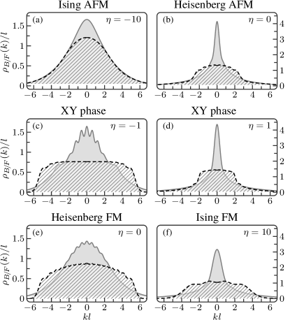
Figure 4: Momentum distributions of nine bosons (solid) and eight fermions (dashed) in a harmonic trap for $g_{BF}<0$ (left column) and $g_{BF}>0$ (right column). See the text for a description of the different phases. $l$ is the harmonic oscillator length.

IV Momentum distributions and occupancies

The momentum distributions and the occupancies of the harmonic-trap levels are important observables, which can be measured in the experiment Pagano14 ; Murmann15 ; Meinert16 . These distributions depend strongly on the degree of exchange symmetry of the spatial many-body wave function and can also be used as a probe for the magnetic structure of the spin chain Murmann15 ; Deuretzbacher16 ; Decamp16 . We therefore expect very different momentum distributions and trap-level occupancies in the different phases of the Bose-Fermi chain as will be shown in the following.

Momentum distributions of nine bosons (solid) and eight fermions (dashed) are shown in Fig. 4. Both momentum distributions resemble Gaussian distributions in the Ising AFM phase, Fig. 4(a), as expected for a Wigner crystal Deuretzbacher10 . This is a result of the comparatively large distance between the particles of the same kind; see Fig. 3(a). In the Heisenberg AFM phase, Fig. 4(b), the bosonic and fermionic distributions look like those of the corresponding spin-1/2 particles Yang15 ; Deuretzbacher16 . By contrast, in the Heisenberg FM phase, Fig. 4(e), both distributions are much broader, as expected for the highest excited states of the corresponding spin-1/2 particles Deuretzbacher16 . Indeed, the FM ground state of the Heisenberg Hamiltonian (17) for $J_{i}^{(BF)}<0$ is the highest excited state for $J_{i}^{(BF)}>0$. Moreover, the ground state of Eq. (II) for $J_{i}^{(BB)}=10\,J_{i}^{(BF)}<0$, which has the momentum distribution shown in Fig. 4(a), is the highest excited state for $J_{i}^{(BB)}=10\,J_{i}^{(BF)}>0$ and the ground state for $J_{i}^{(BB)}=J_{i}^{(BF)}<0$, which has the momentum distribution shown in Fig. 4(c), is the highest excited state for $J_{i}^{(BB)}=J_{i}^{(BF)}>0$. This is the reason for the broader momentum distributions in the left column of Fig. 4. Finally, in the Ising FM phase, one has a Tonks-Girardeau gas in the center and noninteracting fermions at the edges of the trap, Fig. 3(f). Therefore, one expects that the momentum distributions of that phase resemble those of a Tonks-Girardeau gas and noninteracting fermions, Fig. 4(f). The distributions are, however, broader than those of Fig. 4(b), since the particles are located in a smaller trap volume.

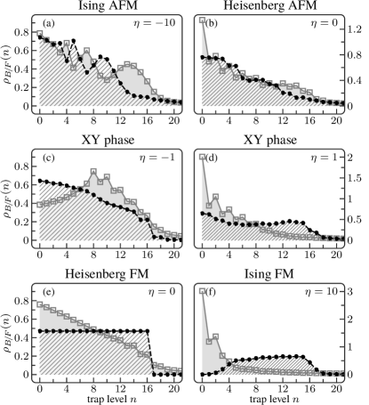
Figure 5: Occupancies of the harmonic-trap levels of nine bosons (solid) and eight fermions (dashed) for $g_{BF}<0$ (left) and $g_{BF}>0$ (right). See the text for a description of the different phases.

The occupancies of the harmonic-trap levels of nine bosons (solid) and eight fermions (dashed) are shown in Fig. 5. In the Ising AFM phase, Fig. 5(a), both occupancies oscillate out of phase around the same average broad distribution. The higher oscillator orbitals ($n>10$) are preferably occupied by the bosons, since the bosonic density is broader [Fig. 3(a)]. The separation of the bosons from the fermions in the Ising FM phase is also manifest in the occupancies, Fig. 5(f). The bosons preferably occupy the lower oscillator orbitals ($n<4$) and the fermions the higher ones ($n>4$). In the Heisenberg AFM phase, Fig. 5(b), the bosonic and fermionic occupancies are almost equal. By contrast, in the Heisenberg FM phase, Fig. 5(e), the fermions occupy the lowest 17 orbitals with $8/17=0.47$ fermions, whereas the bosonic distribution decreases roughly linearly. Finally, once again, the occupancies in the XY phases, Figs. 5(c,d), resemble the behavior of the corresponding densities, Figs. 3(c,d).

In closing this section, we note that the variance of the total momentum distribution, $\langle k^{2}\rangle=\int dkk^{2}(\rho_{F}(k)+\rho_{B}(k))=N^{2}/(2l^{2})$, is independent of the pseudospin configuration of the Bose-Fermi chain. Similarly, the total energy of the Bose-Fermi chain, calculated from the total trap-level occupancies, $\sum_{n=0}^{\infty}(n+1/2)(\rho_{F}(n)+\rho_{B}(n))=N^{2}/2$, is independent of the configuration of the bosons and fermions. This follows from the fact that all pseudospin configurations have the same total energy at $g_{BB}=g_{BF}=\infty$ and from the virial theorem.

V Summary

We have presented a spin-chain model for Bose-Fermi mixtures with nearly infinite BB and BF $\delta$ interactions. The model is based on a mapping to states of the form $|m_{1},\dotsc,m_{N}\rangle$ with $m_{i}=B,F$ and to the wave function of spinless noninteracting fermions. We checked the model by comparing with an exact diagonalization of the full few-body Hamiltonian in the strongly interacting regime. Using the spin-chain model, we determined the ground-state phases of the Bose-Fermi mixture and calculated the densities, momentum distributions, and occupancies of the harmonic-trap levels for up to 17 particles. We found, in particular, AFM and FM order and a demixing of the bosons and fermions. However, we found no demixing for equally strong BB and BF interactions in agreement with earlier calculations Imambekov06 .

Appendix A Sector Wave Functions and Permutations

A.1 Sector wave functions

In the regime of infinite BB and BF repulsion, $g_{BB}=g_{BF}=\infty$, the many-body wave function must vanish whenever two particle coordinates are equal, i.e., $\psi(z_{1},\dotsc,z_{N})=0$ if $z_{i}=z_{j}$. This condition is fulfilled by the wave function of $N$ spinless noninteracting fermions, $\psi_{F}$, but also by its absolute value $|\psi_{F}|$, which describes $N$ spinless bosons with infinite $\delta$ repulsion Girardeau60 . Additionally, we may restrict $|\psi_{F}|$ to a particular sector of the configuration space $\mathbb{R}^{N}$, $z_{P(1)}<\dotsb<z_{P(N)}$, in order to describe spinless distinguishable particles with infinite $\delta$ repulsion and particle ordering $z_{P(1)}<\dotsb<z_{P(N)}$. Here, $P$ denotes an arbitrary permutation of $\underline{N}=\{1,\dotsc,N\}$. The resulting wave function, denoted by $|P\rangle$, is given by Deuretzbacher08

$$\langle z_{1},\dotsc,z_{N}|P\rangle=\sqrt{N!}\,\theta(z_{P(1)},\dotsc,z_{P(N)})|\psi_{F}|.$$ (20)

Here, $\theta(z_{P(1)},\dotsc,z_{P(N)})=1$ if $z_{P(1)}<\dotsb<z_{P(N)}$ and zero otherwise.

The sector wave functions (20) are by definition orthonormal, i.e., $\langle P|P^{\prime}\rangle=\delta_{P,P^{\prime}}$, and they have further favorable properties. For example, the action of a permutation operator $\hat{P}$ on a sector wave function $|P^{\prime}\rangle$ is given by Deuretzbacher16

$$\hat{P}|P^{\prime}\rangle=|P\circ P^{\prime}\rangle.$$ (21)

The permutation operator $\hat{P}$ of a permutation $P$ acts on a many-body state $|\alpha_{1},\dotsc,\alpha_{N}\rangle$ in the following way:

$$\hat{P}|\alpha_{1}\rangle_{1}\dotsm|\alpha_{N}\rangle_{N}=|\alpha_{1}\rangle_{P(1)}\dotsm|\alpha_{N}\rangle_{P(N)}.$$ (22)

That is, $\hat{P}$ permutes the particle indices of a many-body state according to the prescription $1\rightarrow P(1),\dotsc,N\rightarrow P(N)$.

To describe a Bose-Fermi mixture with infinite BB and BF repulsion, ${g_{BB}=g_{BF}=\infty}$, one has to symmetrize the sector wave functions $|P\rangle$ with respect to the bosonic coordinates, $z_{1},\dotsc,z_{N_{B}}$, and to antisymmetrize with respect to the fermionic ones, $z_{N_{B}+1},\dotsc,z_{N}$. We therefore define Fang11

$$\hat{P}|B,\dotsc,B,F,\dotsc,F\rangle\equiv\sqrt{N_{B}!N_{F}!}\,S_{+}S_{-}\,|P^{-1}\rangle.$$ (23)

Here, $S_{+}=(1/N_{B}!)\sum_{P^{\prime}}\hat{P}^{\prime}$ is a symmetrization operator, where the sum runs over all permutations $P^{\prime}$ of $\underline{N_{B}}=\{1,\dotsc,N_{B}\}$, $S_{-}=(1/N_{F}!)\sum_{P^{\prime\prime}}(-1)^{P^{\prime\prime}}\hat{P}^{\prime\prime}$ is an antisymmetrization operator, where the sum runs over all permutations $P^{\prime\prime}$ of $\underline{N}-\underline{N_{B}}=\{N_{B}+1,\dotsc,N\}$, and $P^{-1}$ is the inverse of the permutation $P$. Furthermore, we specify to use only those initial sector wave functions $|P^{-1}\rangle$, for which the bosonic and fermionic coordinates are each in ascending order. This is necessary, since otherwise two sector wave functions, which differ only by the transposition of two fermionic coordinates, would have a different sign. The requirement is fulfilled if we move the $B$ at position $N_{B}$ in the initial state $|B,\dotsc,B,F,\dotsc,F\rangle$ to the new position $i_{N_{B}}$ with $N_{B}\leq i_{N_{B}}\leq N$, the $B$ at position $N_{B}-1$ to the new position $i_{N_{B}-1}$ with $N_{B}-1\leq i_{N_{B}-1}<i_{N_{B}}$, and so forth.

A.2 Permutations

We use the cycle notation to specify a permutation. For example, the permutation $P_{(\alpha,\beta,\gamma)}$ permutes the numbers $\alpha,\beta,\gamma$ according to the prescription $\alpha\rightarrow\beta\rightarrow\gamma\rightarrow\alpha$. Moreover, we neglect the parentheses if a permutation consists of only one cycle, i.e., $P_{(\alpha,\beta,\gamma)}=P_{\alpha,\beta,\gamma}$. The corresponding unitary operator that permutes the particle indices $\alpha,\beta,\gamma$ of a many-body state according to the same rule is denoted by $\hat{P}_{\alpha,\beta,\gamma}$. We also note that a cyclic permutation of $\alpha$, $\beta$, and $\gamma$ does not change the cycle, i.e., $P_{\alpha,\beta,\gamma}=P_{\gamma,\alpha,\beta}=P_{\beta,\gamma,\alpha}$.

The cycle $P_{\alpha,\beta,\gamma}$ is the composition of two transpositions $P_{\alpha,\beta}$ and $P_{\beta,\gamma}$, $P_{\alpha,\beta,\gamma}=P_{\alpha,\beta}\circ P_{\beta,\gamma}$. The corresponding cycle operator $\hat{P}_{\alpha,\beta,\gamma}$ is the product of two transposition operators $\hat{P}_{\alpha,\beta}$ and $\hat{P}_{\beta,\gamma}$, $\hat{P}_{\alpha,\beta,\gamma}=\hat{P}_{\alpha,\beta}\hat{P}_{\beta,\gamma}$. The inverse of the cycle operator $\hat{P}_{\alpha,\beta,\gamma}$ is therefore given by $\hat{P}_{\alpha,\beta,\gamma}^{-1}=(\hat{P}_{\alpha,\beta}\hat{P}_{\beta,\gamma})^{-1}=\hat{P}_{\gamma,\beta}\hat{P}_{\beta,\alpha}=\hat{P}_{\gamma,\beta,\alpha}$, i.e., the particle indices appear in the inverse cycle operator in the inverse order.

The identity permutation is denoted by “$\mathrm{id}$” and the corresponding operator by $\openone$. A particular cycle is the loop permutation, which is defined by

$$P_{i,\dotsc,j}=\left\{\begin{aligned} &P_{i,i+1,\dotsc,j-1,j}\quad\text{for}\quad i<j\\ &\mathrm{id}\mspace{106.5mu}\text{for}\quad i=j\\ &P_{i,i-1,\dotsc,j+1,j}\quad\text{for}\quad i>j.\end{aligned}\right.$$ (24)

The loop permutation is therefore a composition of transpositions of consecutive integers, $P_{i,\dotsc,j}=P_{i,i+1}\circ P_{i+1,i+2}\circ\,\dotsb\,\circ P_{j-2,j-1}\circ P_{j-1,j}$ (assuming $i<j$) and the loop permutation operator $\hat{P}_{i,\dotsc,j}$ is a product of transpositions of neighboring particles, $\hat{P}_{i,\dotsc,j}=\hat{P}_{i,i+1}\hat{P}_{i+1,i+2}\dotsm\hat{P}_{j-2,j-1}\hat{P}_{j-1,j}$. The loop permutation operator $\hat{P}_{i,\dotsc,j}$ therefore moves the particle at position $j$ to position $i$.

A.3 Basis of a two-boson two-fermion mixture

The goal of this section is to clarify definition (23). A basis of a mixture of two bosons and two fermions (2B2F mixture) is given by

$$\mspace{-30.0mu}|B,B,F,F\rangle,\quad|B,F,B,F\rangle,\quad|B,F,F,B\rangle,$$

$$\mspace{-30.0mu}|F,B,F,B\rangle,\mspace{20.0mu}|F,F,B,B\rangle,\mspace{20.0mu}|F,B,B,F\rangle.$$ (25)

The first basis state is, according to Eq. (23), constructed by means of the sector wave function $|\mathrm{id}\rangle$ that corresponds to the identity permutation,

$$|B,B,F,F\rangle=\frac{1}{2}(\openone+\hat{P}_{1,2})(\openone-\hat{P}_{3,4})|\mathrm{id}\rangle.$$ (26)

The second basis state is obtained from the first one by transposing the second and third particle. Therefore, we obtain

$$|B,F,B,F\rangle = \hat{P}_{2,3}|B,B,F,F\rangle$$ (27)

$$= \frac{1}{2}(\openone+\hat{P}_{1,2})(\openone-\hat{P}_{3,4})|P_{2,3}\rangle.$$

The third basis state is obtained from the first one by moving the second $B$ to the fourth position. This is achieved by applying the loop permutation operator $\hat{P}_{4,3,2}$. The inverse of this loop permutation operator is given by $\hat{P}_{4,3,2}^{-1}=\hat{P}_{2,3,4}$. We therefore obtain, using Eq. (23),

$$|B,F,F,B\rangle = \hat{P}_{4,3,2}|B,B,F,F\rangle$$ (28)

$$= \frac{1}{2}(\openone+\hat{P}_{1,2})(\openone-\hat{P}_{3,4})|P_{2,3,4}\rangle.$$

Note that the bosonic ($z_{1},z_{2}$) and fermionic coordinates ($z_{3},z_{4}$) are each in ascending order in the initial sector wave function $|P_{2,3,4}\rangle$, since $z_{1}<z_{3}<z_{4}<z_{2}$, as required.

The fourth basis state is obtained from the first one by moving the second $B$ to the fourth position and then the first $B$ to the second position, i.e., by applying $\hat{P}_{1,2}\hat{P}_{4,3,2}=\hat{P}_{1,2,4,3}$. Using $\hat{P}_{1,2,4,3}^{-1}=\hat{P}_{3,4,2,1}=\hat{P}_{2,1,3,4}$ we obtain

$$|F,B,F,B\rangle=\frac{1}{2}(\openone+\hat{P}_{1,2})(\openone-\hat{P}_{3,4})|P_{2,1,3,4}\rangle.$$ (29)

The fifth basis state is obtained from the first one by moving the second $B$ to the fourth position and then the first $B$ to the third position, i.e., by applying $\hat{P}_{3,2,1}\hat{P}_{4,3,2}=\hat{P}_{(1,3)(2,4)}$. Using $\hat{P}_{(1,3)(2,4)}^{-1}=\hat{P}_{(1,3)(2,4)}$ we obtain

$$|F,F,B,B\rangle=\frac{1}{2}(\openone+\hat{P}_{1,2})(\openone-\hat{P}_{3,4})|P_{(1,3)(2,4)}\rangle.$$ (30)

The sixth basis state is finally obtained from the first one by moving the second $B$ to the third position and then the first $B$ to the second position, i.e., by applying $\hat{P}_{2,1}\hat{P}_{3,2}=\hat{P}_{1,2,3}$. Using $\hat{P}_{1,2,3}^{-1}=\hat{P}_{3,2,1}$ we obtain

$$|F,B,B,F\rangle=\frac{1}{2}(\openone+\hat{P}_{1,2})(\openone-\hat{P}_{3,4})|P_{3,2,1}\rangle.$$ (31)

Appendix B Effective Hamiltonian

Here, we perform a perturbative calculation of a strongly interacting 2B1F mixture up to linear order in $1/g_{BB}$ and $1/g_{BF}$. The matrix elements of the Hamiltonian in the degenerate ground-state manifold are shown to agree with Eq. (3). The basis states of the 2B1F mixture are [see Eq. (23)]

$$|1\rangle \!\!:=|B,B,F\rangle \!\!=\frac{1}{\sqrt{2}}(\openone+\hat{P}_{1,2})|\mathrm{id}\rangle,$$ (32)

$$|2\rangle \!\!:=|B,F,B\rangle \!\!=\frac{1}{\sqrt{2}}(\openone+\hat{P}_{1,2})|P_{2,3}\rangle,$$ (33)

$$|3\rangle \!\!:=|F,B,B\rangle \!\!=\frac{1}{\sqrt{2}}(\openone+\hat{P}_{1,2})|P_{3,2,1}\rangle.$$ (34)

The Hamiltonian of the 2B1F mixture is given by [see Eq. (1)]

$$H = \sum_{i=1}^{3}\left[-\frac{\hbar^{2}}{2M}\frac{\partial^{2}}{\partial z_{i}^{2}}+V(z_{i})\right]+g_{BB}\delta(z_{1}-z_{2})$$ (35)

$$+\>g_{BF}\delta(z_{1}-z_{3})+g_{BF}\delta(z_{2}-z_{3}).$$

The matrix element $\langle 1|H|1\rangle$ is therefore given by

$$\langle 1|H|1\rangle=\frac{1}{2}\langle\mathrm{id}|(\openone+\hat{P}_{1,2})H(\openone+\hat{P}_{1,2})|\mathrm{id}\rangle.$$ (36)

$H$ is symmetric under the exchange of the first and second particle. $H$ therefore commutes with $(\openone+\hat{P}_{1,2})$. Moreover, $(\openone+\hat{P}_{1,2})(\openone+\hat{P}_{1,2})=2(\openone+\hat{P}_{1,2})$ and therefore

$$\langle 1|H|1\rangle=\langle\mathrm{id}|H|\mathrm{id}\rangle+\langle\mathrm{id}|H|P_{1,2}\rangle.$$ (37)

Let us calculate an arbitrary matrix element $\langle P|H|P^{\prime}\rangle$ in the vicinity of $(1/g_{BB},1/g_{BF})=(0,0)$. Performing a Taylor expansion up to first order in $1/g_{BB}$ and $1/g_{BF}$, we obtain Deuretzbacher14

$$\mspace{-50.0mu}\langle P|H|P^{\prime}\rangle=E_{F}\delta_{P,P^{\prime}}$$

$$\mspace{-30.0mu}-\frac{1}{g_{BB}}\lim_{g_{BB}\rightarrow+\infty}\left(g_{BB}^{2}\langle P^{(g_{BB})}|\frac{dH}{dg_{BB}}|P^{\prime(g_{BB})}\rangle\right)$$

$$\mspace{-30.0mu}-\frac{1}{g_{BF}}\lim_{g_{BF}\rightarrow+\infty}\left(g_{BF}^{2}\langle P^{(g_{BF})}|\frac{dH}{dg_{BF}}|P^{\prime(g_{BF})}\rangle\right)$$ (38)

with $\frac{dH}{dg_{BB}}=\delta(z_{1}-z_{2})$ and $\frac{dH}{dg_{BF}}=\delta(z_{1}-z_{3})+\delta(z_{2}-z_{3})$. $|P^{(g)}\rangle$ is the ground state of $N$ spinless bosons with strong $\delta$ repulsion restricted to the sector $z_{P(1)}<\dotsb<z_{P(N)}$ Deuretzbacher14 . Furthermore, using the boundary condition

$$\mspace{-30.0mu}\left(\frac{\partial}{\partial z_{i}}-\frac{\partial}{\partial z_{j}}\right)\psi\big{|}_{z_{i}=z_{j}+}-\left(\frac{\partial}{\partial z_{i}}-\frac{\partial}{\partial z_{j}}\right)\psi\big{|}_{z_{i}=z_{j}-}$$

$$\mspace{-10.0mu}=\frac{2Mg}{\hbar^{2}}\psi\big{|}_{z_{i}=z_{j}},$$ (39)

one finds

$$\lim_{g\rightarrow+\infty}\left(g^{2}\langle P^{(g)}|\delta(z_{i}-z_{j})|P^{\prime(g)}\rangle\right)=C_{i,j}^{P,P^{\prime}}$$ (40)

with

$$\mspace{-50.0mu}C_{i,j}^{P,P^{\prime}} \!\!= \!\frac{N!\hbar^{4}}{M^{2}}\int dz_{1}\dotsi dz_{N}\,\delta(z_{i}-z_{j})\left|\frac{\partial\psi_{F}}{\partial z_{i}}\right|^{2}$$ (41)

$$\!\times\theta(z_{P(1)},\dotsc,z_{P(N)})\theta(z_{P^{\prime}(1)},\dotsc,z_{P^{\prime}(N)}).$$

As a result, we obtain

$$\langle P|H|P^{\prime}\rangle=E_{F}\delta_{P,P^{\prime}}-\frac{1}{g_{BB}}C_{1,2}^{P,P^{\prime}}\!\!-\frac{1}{g_{BF}}\!\left(\!C_{1,3}^{P,P^{\prime}}\!\!+C_{2,3}^{P,P^{\prime}}\right)\!.$$ (42)

Applying this to the matrix element $\langle 1|H|1\rangle$, we get

$$\langle 1|H|1\rangle=E_{F}-2J_{1}^{(BB)}-J_{2}^{(BF)},$$ (43)

since $C_{1,2}^{\mathrm{id},\mathrm{id}}=C_{1,2}^{\mathrm{id},P_{1,2}}=C_{1}$, $C_{2,3}^{\mathrm{id},\mathrm{id}}=C_{2}$, and $C_{1,3}^{\mathrm{id},\mathrm{id}}=C_{1,3}^{\mathrm{id},P_{1,2}}=C_{2,3}^{\mathrm{id},P_{1,2}}=0$. In a similar way we obtain

$$\langle 1|H|2\rangle=\langle\mathrm{id}|H|P_{2,3}\rangle+\langle\mathrm{id}|H|P_{1,2,3}\rangle=-J_{2}^{(BF)},$$ (44)

since only $C_{2,3}^{\mathrm{id},P_{2,3}}=C_{2}$ is nonzero. For the next matrix element, we get

$$\langle 1|H|3\rangle=\langle\mathrm{id}|H|P_{1,3}\rangle+\langle\mathrm{id}|H|P_{3,2,1}\rangle=0,$$ (45)

since $C_{i,j}^{\mathrm{id},P_{1,3}}=C_{i,j}^{\mathrm{id},P_{3,2,1}}=0$ for all $1\leq i<j\leq 3$. The next matrix element becomes

$$\langle 2|H|2\rangle = \langle P_{2,3}|H|P_{2,3}\rangle+\langle P_{2,3}|H|P_{1,2,3}\rangle$$ (46)

$$= E_{F}-J_{1}^{(BF)}-J_{2}^{(BF)},$$

since only $C_{1,3}^{P_{2,3},P_{2,3}}=C_{1}$ and $C_{2,3}^{P_{2,3},P_{2,3}}=C_{2}$ are nonzero. Finally we obtain

$$\langle 2|H|3\rangle=\langle P_{2,3}|H|P_{1,3}\rangle+\langle P_{2,3}|H|P_{3,2,1}\rangle=-J_{1}^{(BF)}$$ (47)

and

$$\langle 3|H|3\rangle = \langle P_{3,2,1}|H|P_{1,3}\rangle+\langle P_{3,2,1}|H|P_{3,2,1}\rangle$$ (48)

$$= E_{F}-2J_{2}^{(BB)}-J_{1}^{(BF)},$$

since only $C_{1,3}^{P_{2,3},P_{3,2,1}}=C_{1,3}^{P_{3,2,1},P_{3,2,1}}=C_{1}$ and $C_{1,2}^{P_{3,2,1},P_{1,3}}=C_{1,2}^{P_{3,2,1},P_{3,2,1}}=C_{2}$ are nonzero. The same matrix elements are obtained using $H_{\mathrm{eff}}$, given by Eq. (3).

Appendix C One-Body Density Matrix

Here, we calculate the matrix elements of the bosonic and fermionic one-body density matrices of a 1B2F mixture. The basis states of the 1B2F mixture are [see Eq. (23)]

$$|1\rangle \!\!:=|B,F,F\rangle \!\!=\frac{1}{\sqrt{2}}(\openone-\hat{P}_{2,3})|\mathrm{id}\rangle,$$ (49)

$$|2\rangle \!\!:=|F,B,F\rangle \!\!=\frac{1}{\sqrt{2}}(\openone-\hat{P}_{2,3})|P_{1,2}\rangle,$$ (50)

$$|3\rangle \!\!:=|F,F,B\rangle \!\!=\frac{1}{\sqrt{2}}(\openone-\hat{P}_{2,3})|P_{1,2,3}\rangle.$$ (51)

The bosonic and fermionic one-body density matrix operators read

$$\hat{\rho}_{B}(z,z^{\prime})=|z\rangle_{1}\langle z^{\prime}|_{1}$$ (52)

and

$$\hat{\rho}_{F}(z,z^{\prime})=|z\rangle_{2}\langle z^{\prime}|_{2}+|z\rangle_{3}\langle z^{\prime}|_{3}.$$ (53)

First, we calculate the matrix elements of the bosonic distribution $\hat{\rho}_{B}(z,z^{\prime})$. One finds

$$\langle 1|\hat{\rho}_{B}(z,z^{\prime})|1\rangle=\langle\mathrm{id}|z\rangle_{1}\langle z^{\prime}|_{1}(|\mathrm{id}\rangle-|P_{2,3}\rangle).$$ (54)

Only those matrix elements of the form $\langle\mathrm{id}|z\rangle_{i}\langle z^{\prime}|_{i}|P\rangle$ are nonzero for which $P=P_{i,\dotsc,j}$. We define

$$\rho^{(i,j)}(z,z^{\prime})=\langle\mathrm{id}|z\rangle_{i}\langle z^{\prime}|_{i}|P_{i,\dotsc,j}\rangle.$$ (55)

Using this, we find

$$\mspace{-40.0mu}\langle 1|\hat{\rho}_{B}(z,z^{\prime})|1\rangle=\rho^{(1,1)}(z,z^{\prime})$$

$$\mspace{-20.0mu}=\langle B,F,F|\rho^{(1,1)}(z,z^{\prime})|B\rangle_{1}\langle B|_{1}|B,F,F\rangle.$$ (56)

The next two matrix elements are given by

$$\mspace{-50.0mu}\langle 1|\hat{\rho}_{B}(z,z^{\prime})|2\rangle=\langle\mathrm{id}|z\rangle_{1}\langle z^{\prime}|_{1}(|P_{1,2}\rangle-|P_{3,2,1}\rangle)$$

$$\mspace{-30.0mu}=\rho^{(1,2)}(z,z^{\prime})$$

$$\mspace{-30.0mu}=\langle B,F,F|\rho^{(1,2)}(z,z^{\prime})|B\rangle_{1}\langle B|_{1}\hat{P}_{1,2}|F,B,F\rangle$$ (57)

and

$$\mspace{-60.0mu}\langle 1|\hat{\rho}_{B}(z,z^{\prime})|3\rangle=\langle\mathrm{id}|z\rangle_{1}\langle z^{\prime}|_{1}(|P_{1,2,3}\rangle-|P_{1,3}\rangle)$$

$$\mspace{-40.0mu}=\rho^{(1,3)}(z,z^{\prime})$$

$$\mspace{-40.0mu}=\langle B,F,F|\rho^{(1,3)}(z,z^{\prime})|B\rangle_{1}\langle B|_{1}\hat{P}_{1,2,3}|F,F,B\rangle.$$ (58)

In the next case, we find

$$\langle 2|\hat{\rho}_{B}(z,z^{\prime})|2\rangle=\langle P_{1,2}|z\rangle_{1}\langle z^{\prime}|_{1}(|P_{1,2}\rangle-|P_{3,2,1}\rangle).$$ (59)

It is easy to show that

$$\langle P|z\rangle_{i}\langle z^{\prime}|_{i}|P^{\prime}\rangle=\langle\mathrm{id}|z\rangle_{P^{-1}(i)}\langle z^{\prime}|_{P^{-1}(i)}|P^{-1}\circ P^{\prime}\rangle.$$ (60)

Using this, we find

$$\mspace{-22.0mu}\langle 2|\hat{\rho}_{B}(z,z^{\prime})|2\rangle=\langle\mathrm{id}|z\rangle_{2}\langle z^{\prime}|_{2}(|\mathrm{id}\rangle-|P_{1,3}\rangle)=\rho^{(2,2)}(z,z^{\prime})$$

$$\mspace{-2.0mu}=\langle F,B,F|\rho^{(2,2)}(z,z^{\prime})|B\rangle_{2}\langle B|_{2}|F,B,F\rangle.$$ (61)

In the next case, we obtain

$$\mspace{-50.0mu}\langle 2|\hat{\rho}_{B}(z,z^{\prime})|3\rangle=\langle P_{1,2}|z\rangle_{1}\langle z^{\prime}|_{1}(|P_{1,2,3}\rangle-|P_{1,3}\rangle)$$

$$\mspace{-30.0mu}=\langle\mathrm{id}|z\rangle_{2}\langle z^{\prime}|_{2}(|P_{2,3}\rangle-|P_{3,2,1}\rangle)=\rho^{(2,3)}(z,z^{\prime})$$

$$\mspace{-30.0mu}=\langle F,B,F|\rho^{(2,3)}(z,z^{\prime})|B\rangle_{2}\langle B|_{2}\hat{P}_{2,3}|F,F,B\rangle.$$ (62)

The last matrix element is given by

$$\mspace{-40.0mu}\langle 3|\hat{\rho}_{B}(z,z^{\prime})|3\rangle=\langle P_{1,2,3}|z\rangle_{1}\langle z^{\prime}|_{1}(|P_{1,2,3}\rangle-|P_{1,3}\rangle)$$

$$\mspace{-20.0mu}=\langle\mathrm{id}|z\rangle_{3}\langle z^{\prime}|_{3}(|\mathrm{id}\rangle-|P_{1,2}\rangle)=\rho^{(3,3)}(z,z^{\prime})$$

$$\mspace{-20.0mu}=\langle F,F,B|\rho^{(3,3)}(z,z^{\prime})|B\rangle_{3}\langle B|_{3}|F,F,B\rangle.$$ (63)

One sees that the matrix elements of the bosonic one-body density matrix agree with those of Eqs. (10)–(12). Now, we calculate the matrix elements of the fermionic distribution $\hat{\rho}_{F}(z,z^{\prime})$. The first two matrix elements read

$$\mspace{-10.0mu}\langle 1|\hat{\rho}_{F}(z,z^{\prime})|1\rangle \!\!= \!\!\langle\mathrm{id}|(|z\rangle_{2}\langle z^{\prime}|_{2}+|z\rangle_{3}\langle z^{\prime}|_{3})(|\mathrm{id}\rangle-|P_{2,3}\rangle)=\rho^{(2,2)}(z,z^{\prime})-\rho^{(2,3)}(z,z^{\prime})+\rho^{(3,3)}(z,z^{\prime})-\rho^{(3,2)}(z,z^{\prime})$$ (64)

$$\!\!= \!\!\langle B,F,F|\Bigl{(}\rho^{(2,2)}(z,z^{\prime})|F\rangle_{2}\langle F|_{2}-\rho^{(2,3)}(z,z^{\prime})|F\rangle_{2}\langle F|_{2}\hat{P}_{2,3}$$

$$\mspace{73.0mu}+\rho^{(3,3)}(z,z^{\prime})|F\rangle_{3}\langle F|_{3}-\rho^{(3,2)}(z,z^{\prime})|F\rangle_{3}\langle F|_{3}\hat{P}_{3,2}\Bigr{)}|B,F,F\rangle$$

and

$$\langle 1|\hat{\rho}_{F}(z,z^{\prime})|2\rangle \!\!= \!\!\langle\mathrm{id}|(|z\rangle_{2}\langle z^{\prime}|_{2}+|z\rangle_{3}\langle z^{\prime}|_{3})(|P_{1,2}\rangle-|P_{3,2,1}\rangle)=\rho^{(2,1)}(z,z^{\prime})-\rho^{(3,1)}(z,z^{\prime})$$ (65)

$$\!\!= \!\!\langle B,F,F|\left(\rho^{(2,1)}(z,z^{\prime})|F\rangle_{2}\langle F|_{2}\hat{P}_{2,1}-\rho^{(3,1)}(z,z^{\prime})|F\rangle_{3}\langle F|_{3}\hat{P}_{3,2,1}\right)|F,B,F\rangle.$$

The next matrix element is zero,

$$\langle 1|\hat{\rho}_{F}(z,z^{\prime})|3\rangle=\langle\mathrm{id}|(|z\rangle_{2}\langle z^{\prime}|_{2}+|z\rangle_{3}\langle z^{\prime}|_{3})(|P_{1,2,3}\rangle-|P_{1,3}\rangle)=0.$$ (66)

Using Eq. (60), we obtain for the last three matrix elements

$$\mspace{-44.0mu}\langle 2|\hat{\rho}_{F}(z,z^{\prime})|2\rangle \!\!= \!\!\langle P_{1,2}|(|z\rangle_{2}\langle z^{\prime}|_{2}+|z\rangle_{3}\langle z^{\prime}|_{3})(|P_{1,2}\rangle-|P_{3,2,1}\rangle)=\langle\mathrm{id}|(|z\rangle_{1}\langle z^{\prime}|_{1}+|z\rangle_{3}\langle z^{\prime}|_{3})(|\mathrm{id}\rangle-|P_{1,3}\rangle)$$ (67)

$$\!\!= \!\!\rho^{(1,1)}(z,z^{\prime})+\rho^{(3,3)}(z,z^{\prime})=\langle F,B,F|\left(\rho^{(1,1)}(z,z^{\prime})|F\rangle_{1}\langle F|_{1}+\rho^{(3,3)}(z,z^{\prime})|F\rangle_{3}\langle F|_{3}\right)|F,B,F\rangle,$$

$$\langle 2|\hat{\rho}_{F}(z,z^{\prime})|3\rangle \!\!= \!\!\langle P_{1,2}|(|z\rangle_{2}\langle z^{\prime}|_{2}+|z\rangle_{3}\langle z^{\prime}|_{3})(|P_{1,2,3}\rangle-|P_{1,3}\rangle)=\langle\mathrm{id}|(|z\rangle_{1}\langle z^{\prime}|_{1}+|z\rangle_{3}\langle z^{\prime}|_{3})(|P_{2,3}\rangle-|P_{3,2,1}\rangle)$$

$$\!\!= \!\!\rho^{(3,2)}(z,z^{\prime})-\rho^{(3,1)}(z,z^{\prime})=\langle F,B,F|\!\left(\rho^{(3,2)}(z,z^{\prime})|F\rangle_{3}\langle F|_{3}\hat{P}_{3,2}-\rho^{(3,1)}(z,z^{\prime})|F\rangle_{3}\langle F|_{3}\hat{P}_{3,2,1}\!\right)\!|F,F,B\rangle,$$

and

$$\mspace{-10.0mu}\langle 3|\hat{\rho}_{F}(z,z^{\prime})|3\rangle \!\!= \!\!\langle P_{1,2,3}|(|z\rangle_{2}\langle z^{\prime}|_{2}+|z\rangle_{3}\langle z^{\prime}|_{3})(|P_{1,2,3}\rangle-|P_{1,3}\rangle)=\langle\mathrm{id}|(|z\rangle_{1}\langle z^{\prime}|_{1}+|z\rangle_{2}\langle z^{\prime}|_{2})(|\mathrm{id}\rangle-|P_{1,2}\rangle)$$ (69)

$$\!\!= \!\!\rho^{(1,1)}(z,z^{\prime})-\rho^{(1,2)}(z,z^{\prime})+\rho^{(2,2)}(z,z^{\prime})-\rho^{(2,1)}(z,z^{\prime})$$

$$\!\!= \!\!\langle F,F,B|\Bigl{(}\rho^{(1,1)}(z,z^{\prime})|F\rangle_{1}\langle F|_{1}-\rho^{(1,2)}(z,z^{\prime})|F\rangle_{1}\langle F|_{1}\hat{P}_{1,2}$$

$$\mspace{70.0mu}+\rho^{(2,2)}(z,z^{\prime})|F\rangle_{2}\langle F|_{2}-\rho^{(2,1)}(z,z^{\prime})|F\rangle_{2}\langle F|_{2}\hat{P}_{2,1}\Bigr{)}|F,F,B\rangle.$$

Again, one sees that the matrix elements of the fermionic one-body density matrix agree with those of Eqs. (10)–(12).

References

• (1) M. A. Cazalilla, R. Citro, T. Giamarchi, E. Orignac, and M. Rigol, One dimensional bosons: From condensed matter systems to ultracold gases, Rev. Mod. Phys. 83, 1405 (2011).
• (2) X.-W. Guan, M. T. Batchelor, and C. Lee, Fermi gases in one dimension: From Bethe ansatz to experiments, Rev. Mod. Phys. 85, 1633 (2013).
• (3) T. Kinoshita, T. Wenger, and D. S. Weiss, Observation of a One-Dimensional Tonks-Girardeau Gas, Science 305, 1125 (2004).
• (4) B. Paredes, A. Widera, V. Murg, O. Mandel, S. Fölling, I. Cirac, G. V. Shlyapnikov, T. W. Hänsch, and I. Bloch, Tonks-Girardeau gas of ultracold atoms in an optical lattice, Nature (London) 429, 277 (2004).
• (5) E. Haller, M. Gustavsson, M. J. Mark, J. G. Danzl, R. Hart, G. Pupillo, and H.-C. Nägerl, Realization of an Excited, Strongly Correlated Quantum Gas Phase, Science 325, 1224 (2009).
• (6) G. E. Astrakharchik, J. Boronat, J. Casulleras, and S. Giorgini, Beyond the Tonks-Girardeau Gas: Strongly Correlated Regime in Quasi-One-Dimensional Bose Gases, Phys. Rev. Lett. 95, 190407 (2005).
• (7) T. Kinoshita, T. Wenger, and D. S. Weiss, A quantum Newton’s cradle, Nature (London) 440, 900 (2006).
• (8) F. Serwane, G. Zürn, T. Lompe, T. B. Ottenstein, A. N. Wenz, and S. Jochim, Deterministic Preparation of a Tunable Few-Fermion System, Science 332, 336 (2011).
• (9) G. Zürn, F. Serwane, T. Lompe, A. N. Wenz, M. G. Ries, J. E. Bohn, and S. Jochim, Fermionization of Two Distinguishable Fermions, Phys. Rev. Lett. 108, 075303 (2012).
• (10) G. Zürn, A. N. Wenz, S. Murmann, A. Bergschneider, T. Lompe, and S. Jochim, Pairing in Few-Fermion Systems with Attractive Interactions, Phys. Rev. Lett. 111, 175302 (2013).
• (11) A. N. Wenz, G. Zürn, S. Murmann, I. Brouzos, T. Lompe, and S. Jochim, From Few to Many: Observing the Formation of a Fermi Sea One Atom at a Time, Science 342, 457 (2013).
• (12) S. Murmann, F. Deuretzbacher, G. Zürn, J. Bjerlin, S. M. Reimann, L. Santos, T. Lompe, and S. Jochim, Antiferromagnetic Heisenberg Spin Chain of a Few Cold Atoms in a One-Dimensional Trap, Phys. Rev. Lett. 115, 215301 (2015).
• (13) G. Pagano, M. Mancini, G. Cappellini, P. Lombardi, F. Schäfer, H. Hu, X.-J. Liu, J. Catani, C. Sias, M. Inguscio, and L. Fallani, A one-dimensional liquid of fermions with tunable spin, Nat. Phys. 10, 198 (2014).
• (14) F. Schreck, L. Khaykovich, K. L. Corwin, G. Ferrari, T. Bourdel, J. Cubizolles, and C. Salomon, Quasipure Bose-Einstein Condensate Immersed in a Fermi Sea, Phys. Rev. Lett. 87, 080403 (2001).
• (15) M. Girardeau, Relationship between Systems of Impenetrable Bosons and Fermions in One Dimension, J. Math. Phys. 1, 516 (1960).
• (16) M. D. Girardeau and A. Minguzzi, Soluble Models of Strongly Interacting Ultracold Gas Mixtures in Tight Waveguides, Phys. Rev. Lett. 99, 230402 (2007).
• (17) F. Deuretzbacher, K. Fredenhagen, D. Becker, K. Bongs, K. Sengstock, and D. Pfannkuche, Exact Solution of Strongly Interacting Quasi-One-Dimensional Spinor Bose Gases, Phys. Rev. Lett. 100, 160405 (2008).
• (18) L. Guan, S. Chen, Y. Wang, and Z.-Q. Ma, Exact Solution for Infinitely Strongly Interacting Fermi Gases in Tight Waveguides, Phys. Rev. Lett. 102, 160402 (2009).
• (19) A. G. Volosniev, D. V. Fedorov, A. S. Jensen, M. Valiente, and N. T. Zinner, Strongly interacting confined quantum systems in one dimension, Nat. Commun. 5, 5300 (2014).
• (20) K. A. Matveev and A. Furusaki, Spectral Functions of Strongly Interacting Isospin-1/2 Bosons in One Dimension, Phys. Rev. Lett. 101, 170403 (2008).
• (21) F. Deuretzbacher, D. Becker, J. Bjerlin, S. M. Reimann, and L. Santos, Quantum magnetism without lattices in strongly interacting one-dimensional spinor gases, Phys. Rev. A 90, 013611 (2014).
• (22) A. G. Volosniev, D. Petrosyan, M. Valiente, D. V. Fedorov, A. S. Jensen, and N. T. Zinner, Engineering the dynamics of effective spin-chain models for strongly interacting atomic gases, Phys. Rev. A 91, 023620 (2015).
• (23) L. Yang, L. Guan, and H. Pu, Strongly interacting quantum gases in one-dimensional traps, Phys. Rev. A 91, 043634 (2015).
• (24) P. Massignan, J. Levinsen, and M. M. Parish, Magnetism in Strongly Interacting One-Dimensional Quantum Mixtures, Phys. Rev. Lett. 115, 247202 (2015).
• (25) L. Yang and X. Cui, Effective spin-chain model for strongly interacting one-dimensional atomic gases with an arbitrary spin, Phys. Rev. A 93, 013617 (2016).
• (26) M. Lewenstein, L. Santos, M. A. Baranov, and H. Fehrmann, Atomic Bose-Fermi Mixtures in an Optical Lattice, Phys. Rev. Lett. 92, 050401 (2004).
• (27) L. Mathey and D.-W. Wang, Phase diagrams of one-dimensional Bose-Fermi mixtures of ultracold atoms, Phys. Rev. A 75, 013612 (2007).
• (28) M. A. Cazalilla and A. F. Ho, Instabilities in Binary Mixtures of One-Dimensional Quantum Degenerate Gases, Phys. Rev. Lett. 91, 150403 (2003).
• (29) A. Imambekov and E. Demler, Exactly solvable case of a one-dimensional Bose-Fermi mixture, Phys. Rev. A 73, 021602(R) (2006).
• (30) X.-W. Guan, M. T. Batchelor, and J.-Y. Lee, Magnetic ordering and quantum statistical effects in strongly repulsive Fermi-Fermi and Bose-Fermi mixtures, Phys. Rev. A 78, 023621 (2008).
• (31) B. Fang, P. Vignolo, M. Gattobigio, C. Miniatura, and A. Minguzzi, Exact solution for the degenerate ground-state manifold of a strongly interacting one-dimensional Bose-Fermi mixture, Phys. Rev. A 84, 023626 (2011).
• (32) H. Hu, L. Guan, and S. Chen, Strongly interacting Bose-Fermi mixtures in one dimension, New J. Phys. 18, 025009 (2016).
• (33) A. S. Dehkharghani, F. F. Bellotti, and N. T. Zinner, Analytical and numerical studies of Bose-Fermi mixtures in a one-dimensional harmonic trap, arXiv:1703.01836.
• (34) N. T. Zinner, Strongly interacting mesoscopic systems of anyons in one dimension, Phys. Rev. A 92, 063634 (2015).
• (35) H. Hu, L. Pan, and S. Chen, Strongly interacting one-dimensional quantum gas mixtures with weak $p$-wave interactions, Phys. Rev. A 93, 033636 (2016).
• (36) L. Yang, X.-W. Guan, and X. Cui, Engineering quantum magnetism in one-dimensional trapped Fermi gases with $p$-wave interactions, Phys. Rev. A 93, 051605(R) (2016).
• (37) See the ancillary files at https://arxiv.org/src/1611.04418v4/anc for the Mathematica notebook.
• (38) S. Inouye, M. R. Andrews, J. Stenger, H.-J. Miesner, D. M. Stamper-Kurn, and W. Ketterle, Observation of Feshbach resonances in a Bose-Einstein condensate, Nature (London) 392, 151 (1998).
• (39) M. Olshanii, Atomic Scattering in the Presence of an External Confinement and a Gas of Impenetrable Bosons, Phys. Rev. Lett. 81, 938 (1998).
• (40) In a quasi-1D trap with a tight transverse harmonic confinement with frequency $\omega_{\perp}$, the inverse strength, $1/g$, of the 1D $\delta$ interaction fulfills $2\hbar\omega_{\perp}l_{\perp}/g=l_{\perp}/a_{3D}-C$, with $l_{\perp}=\sqrt{\hbar/(m\omega_{\perp})}$, $a_{3D}$ the bare 3D scattering length, and $C\simeq 1.0326\dotsc$ Olshanii98 . Hence, by changing either $a_{3D}$ or the transversal confinement, $\hbar\omega l/g$ may be adiabatically changed from an initial small positive (Tonks regime) to a small negative value (super-Tonks regime). The super-Tonks state is a highly excited state but remains metastable due to the small overlap with the strongly bound states. Around the confinement-induced resonance, the charge (i.e. density) degrees of freedom are frozen and well approximated by the wave function of spinless noninteracting fermions, while the spin degrees of freedom are described by the spin-chain model.
• (41) F. Deuretzbacher, D. Becker, and L. Santos, Momentum distributions and numerical methods for strongly interacting one-dimensional spinor gases, Phys. Rev. A 94, 023606 (2016).
• (42) N. J. S. Loft, L. B. Kristensen, A. E. Thomsen, A. G. Volosniev, and N. T. Zinner, CONAN—The cruncher of local exchange coefficients for strongly interacting confined systems in one dimension, Comput. Phys. Commun. 209, 171 (2016).
• (43) L. Yang and H. Pu, Bose-Fermi mapping and a multibranch spin-chain model for strongly interacting quantum gases in one dimension: Dynamics and collective excitations, Phys. Rev. A 94, 033614 (2016).
• (44) F. Deuretzbacher, K. Bongs, K. Sengstock, and D. Pfannkuche, Evolution from a Bose-Einstein condensate to a Tonks-Girardeau gas: An exact diagonalization study, Phys. Rev. A 75, 013614 (2007).
• (45) H.-J. Mikeska and A. K. Kolezhuk, One-Dimensional Magnetism, Lect. Notes Phys. 645, 1 (2004).
• (46) F. Meinert, M. Knap, E. Kirilov, K. Jag-Lauber, M. B. Zvonarev, E. Demler, and H.-C. Nägerl, Bloch oscillations in the absence of a lattice, arXiv:1608.08200.
• (47) J. Decamp, J. Jünemann, M. Albert, M. Rizzi, A. Minguzzi, and P. Vignolo, High-momentum tails as magnetic-structure probes for strongly correlated SU($\kappa$) fermionic mixtures in one-dimensional traps, Phys. Rev. A 94, 053614 (2016).
• (48) F. Deuretzbacher, J. C. Cremon, and S. M. Reimann, Ground-state properties of few dipolar bosons in a quasi-one-dimensional harmonic trap, Phys. Rev. A 81, 063616 (2010); Erratum: Ground-state properties of few dipolar bosons in a quasi-one-dimensional harmonic trap [Phys. Rev. A 81, 063616 (2010)] 87, 039903(E) (2013).