Approximated structured pseudospectra

Abstract

Pseudospectra and structured pseudospectra are important tools for the analysis of matrices. Their computation, however, can be very demanding for all but small matrices. A new approach to compute approximations of pseudospectra and structured pseudospectra, based on determining the spectra of many suitably chosen rank-one or projected rank-one perturbations of the given matrix is proposed. The choice of rank-one or projected rank-one perturbations is inspired by Wilkinson’s analysis of eigenvalue sensitivity. Numerical examples illustrate that the proposed approach gives much better insight into the pseudospectra and structured pseudospectra than random or structured random rank-one perturbations with lower computational burden. The latter approach is presently commonly used for the determination of structured pseudospectra.

1 Introduction

Many applications in science and engineering require knowledge of the location of some or all eigenvalues of a matrix and the sensitivity of the eigenvalues to perturbations of the matrix. The sensitivity can be studied with the aid of the eigenvalue condition number, based on particular rank-one perturbations of the matrix, as described by Wilkinson [23, Chapter 2], or by computing pseudospectra. Let $\Lambda(A)$ denote the spectrum of the matrix $A\in\mathbb{C}^{n\times n}$. The $\varepsilon$-pseudospectrum of the matrix $A$ is defined as

$$\Lambda_{\varepsilon}(A):=\left\{\lambda\in\mathbb{C}\colon\lambda\in\Lambda(A+E),~{}~{}E\in\mathbb{C}^{n\times n},~{}~{}\|E\|\leq\varepsilon\right\}$$ (1.1)

for some $\varepsilon>0$. An insightful discussion of the $\varepsilon$-pseudospectrum and many applications are presented by Trefethen and Embree [22]. The matrix norm $\|\cdot\|$ in (1.1) often is chosen to be the spectral norm. However, it will be convenient to instead use the Frobenius norm $\|\cdot\|_{F}$ in the present paper. Thus, for $E=[e_{ij}]_{i,j=1}^{n}\in\mathbb{C}^{n\times n}$, we have $\|E\|_{F}=\sqrt{\sum_{i,j=1}^{n}|e_{ij}|^{2}}$. The set (1.1) depends on the choice of matrix norm, however, this dependence often is not important in applications when one is interested in determining which eigenvalues of the matrix $A$ are most sensitive to perturbations.

Algorithms for eigenvalue computations that respect the matrix structure may yield higher accuracy and require less computing time than structure-ignoring methods. They also may preserve eigenvalue symmetries in finite-precision arithmetic. A structure-respecting eigenvalue algorithm is said to be strongly backward stable, if the computed eigenvalues are exact eigenvalues of a slightly perturbed matrix with the same structure as the original matrix; see, e.g., Bunch [6]. To assess the numerical properties of a structure-respecting eigenvalue algorithm suitable measures of the sensitivity of the eigenvalues should be used in order not to overestimate the worst-case effect of perturbations. These measures include structured condition numbers, see Higham and Higham [12] and Karow et al. [15], as well as the structured $\varepsilon$-pseudospectrum. The latter can be applied to measure the sensitivity of the eigenvalues of a structured matrix to similarly structured perturbations. It is defined as follows. Let ${{\mathcal{S}}}$ denote the subset of matrices in $\mathbb{C}^{n\times n}$ with a particular structure, such as bandedness, Toeplitz, Hankel, or Hamiltonian. Then, for some $\varepsilon>0$, the structured $\varepsilon$-pseudospectrum of a matrix $A\in{{\mathcal{S}}}$ is given by

$$\Lambda_{\varepsilon}^{{\mathcal{S}}}(A):=\left\{\lambda\in\mathbb{C}\colon\lambda\in\Lambda(A+E),~{}~{}E\in{{\mathcal{S}}},~{}~{}\|E\|\leq\varepsilon\right\};$$ (1.2)

see, e.g., [5, 11, 21] for discussions and illustrations.

The computation of the (standard) $\varepsilon$-pseudospectrum (1.1) for a large or moderately sized matrix $A\in\mathbb{C}^{n\times n}$ for a fixed $\varepsilon>0$ can be very time-consuming. For instance, when the norm $\|\cdot\|$ in (1.1) is the spectral norm, approximations of the $\varepsilon$-pseudospectrum often are determined by computing the smallest singular value of many matrices of the form $A-zI_{n}$, where $I_{n}\in\mathbb{C}^{n\times n}$ denotes the identity matrix and $z\in\mathbb{C}$. If the smallest singular value is smaller than or equal to $\varepsilon$, then $z$ belongs to the set (1.1). These computations are very demanding unless $A$ is small. To reduce the computational burden somewhat, it is suggested in [25, 22] that one first computes the Schur factorization $A=URU^{H}$ and then determines the smallest singular value of the matrix $R-zI_{n}$ for many $z$-values in $\mathbb{C}$. Here $U\in\mathbb{C}^{n\times n}$ is a unitary matrix, $R\in\mathbb{C}^{n\times n}$ an upper triangular matrix, and the superscript ^H denotes transposition and complex conjugation. Nevertheless, the computational task is substantial also when applying the Schur factorization of a moderately sized or large matrix $A$. Moreover, the Schur factorization of $A$ cannot be applied for the computation of the structured $\varepsilon$-pseudospectrum (1.2). In fact, there are few methods available for computing the structured $\varepsilon$-pseudospectrum besides plotting the spectra of matrices $A\in\mathbb{C}^{n\times n}$ with structured random perturbations. Similarly, there are few methods available for determining the stability radius under structured perturbations. In fact, the computation of structured $\varepsilon$-pseudospectra has become an established tool in gaining insight into behavior of matrix-based models in dynamical system theory under structured perturbations. We recall that the (structured) stability radius is the smallest value of $\varepsilon$ for which a (structured) $\varepsilon$-pseudospectrum contour reaches the imaginary axis and defines the norm of the smallest (structured) perturbation that destroys the (structured) stability, that is, having all the eigenvalues confined to $\mathbb{C}^{-}$. Just as the spectral abscissa of a matrix provides a measure of its stability, that is, the asymptotic decay of associated dynamical systems, so does the (structured) $\varepsilon$-pseudospectral abscissa, i.e. the maximal real part of points of the (structured) $\varepsilon$-pseudospectrum provides a measure of robust (structured) stability, where by robust we mean with respect to (structured) perturbations of the matrix. The computations of these quantities remain significant computational challenges to date.

The high computational burden of computing standard (unstructured) pseudospectra has spurred the development of algorithms that can be executed efficiently on a parallel computer; see, e.g., Bekas and Gallopoulos [3] and Mezher and Philippe [16]. We propose a different approach to speed up the computations, that also can be applied to the determination of structured pseudospectra. The given matrix $A\in\mathbb{C}^{n\times n}$ is modified by a sequence of rank-one matrices that are known to yield large perturbations of the eigenvalues according to Wilkinson’s analysis [23, Chapter 2]. Already fairly few rank-one matrices provide insight into the $\varepsilon$-pseudospectrum and when different components of the pseudospectrum coalesce. Computed examples illustrate that the number of our chosen rank-one matrices required to gain knowledge of the $\varepsilon$-pseudospectrum is much smaller than when random rank-one perturbations are used. Our method can be used to inexpensively compute approximated standard (unstructured) pseudospectra when available software tools, such as Eigtool [24] and Seigtool [14], are too expensive to use.

To determine approximations of structured pseudospectra, we project the rank-one matrices suggested by Wilkinson’s analysis onto the set of matrices with desired structure. The computations with our approach can be implemented efficiently on parallel computers, but we will not pursue this aspect in the present paper.

We remark that Karow [13] has analyzed structured pseudospectra when the underlying norm is unitarily invariant. The distance to standard and structured defectivity is not considered in [13]. Also the computational approach of the present paper is new. Rump [21] has characterized the structured pseudospectrum for some structures, such as Toeplitz, and has by means of computer-assisted proofs shown that the structured $\varepsilon$-pseudospectrum (1.2) is quite similar to the standard $\varepsilon$-pseudospectrum (1.1) when there is no zero-structure such as bandedness. Rump’s analysis does not apply to banded Toeplitz matrices. A linearly convergent algorithm for the computation of the structured $\varepsilon$-pseudospectral abscissa and radius of a Toeplitz matrix, and for determining sections of $\Lambda_{\varepsilon}^{{\mathcal{S}}}(A)$ near extremal points is described in [8]. Computations with this algorithm generally are time-consuming.

This paper is organized as follows. Section 2 discusses rank-one perturbations and presents some background material. In Section 3, we provide formulas for eigenvalue structured condition numbers and for the maximal structured perturbations for Toeplitz and Hamiltonian structures. These results are applied in Section 4 in the design of our approach for the inexpensive computation of approximated unstructured and structured pseudospectra. Numerical examples are presented in Section 5, and conclusions are provided in Section 6.

2 Rank-one perturbations and structured matrices

The points in a structured $\varepsilon$-pseudospectrum (1.2) are exact eigenvalues of a nearby matrix in ${{\mathcal{S}}}$. This suggests that we may use standard results from the literature on eigenvalue sensitivity to infinitely small structured perturbations. The structured condition number of an eigenvalue $\lambda$ of $A$ is a first-order measure of the worst-case effect on $\lambda$ of perturbations with the same structure as $A$. The structured condition numbers used in this paper can easily be computed when endowing the subspace of matrices with the Frobenius norm.

First consider an unstructured matrix $A\in\mathbb{C}^{n\times n}$ and assume that it has the simple eigenvalue $\lambda$ with unit right and left eigenvectors $x$ and $y$, respectively. Let $E\in\mathbb{C}^{n\times n}$ have norm $\|E\|_{F}=1$ and assume that $\varepsilon>0$ is small enough so that the eigenvalue $\lambda_{E}(t)$ of $A+tE$ exists and is unique for all $0\leq t<\varepsilon$. Then

$$\lambda_{E}(t)=\lambda+\frac{y^{H}Ex}{y^{H}x}t+{\mathcal{O}}(t^{2});$$

see Wilkinson [23, Chapter 2] for details. We have

$$\left|\frac{y^{H}Ex}{y^{H}x}\right|\leq\frac{1}{|y^{H}x|}$$

with equality for

$$E:=\eta\,yx^{H}$$ (2.1)

for any unimodular $\eta\in\mathbb{C}$. We refer to matrices of the form (2.1) as Wilkinson perturbations and to the set

$${{\mathcal{D}}}(\lambda,t):=\left\{z\in\mathbb{C}:|z-\lambda|\leq\frac{1}{|y^{H}x|}t\right\}$$ (2.2)

as the Wilkinson disk associated with $\lambda$ of radius $t\geq 0$. The condition number of the eigenvalue $\lambda$ is defined as

$$\kappa(\lambda):=\frac{1}{|y^{H}x|}.$$ (2.3)

We turn to structured matrices in a set ${{\mathcal{S}}}\,{\scriptscriptstyle{\begin{subarray}{c}\subset\\ \neq\end{subarray}}}\,\mathbb{C}^{n\times n}$ and consider structured perturbations in ${{\mathcal{S}}}$. Let $M|_{{\mathcal{S}}}$ denote the matrix in ${\mathcal{S}}$ closest to $M\in\mathbb{C}^{n\times n}$ with respect to the Frobenius norm. This projection is used in the numerator of the eigenvalue condition number for structured perturbations; see [17, 18] and Section 3. In particular, the condition number for structured perturbations is smaller than the condition number for unstructured perturbations. We also will use the normalized projection,

$$M|_{\widehat{{\mathcal{S}}}}:=\frac{M|_{\mathcal{S}}}{\|M|_{\mathcal{S}}\|_{F}}\;.$$

In this paper, we are mainly concerned with banded or general Toeplitz structure, ${{\mathcal{S}}}:={{\mathcal{T}}}$, and Hamiltonian structure, ${{\mathcal{S}}}:={{\mathcal{H}}}$. Toeplitz matrices arise in many applications including the solution of ordinary differential equations. It is interesting to investigate the sensitivity of the eigenvalues of a Toeplitz matrix with respect to finite structure-preserving perturbations and, in particular, the sensitivity of the rightmost eigenvalue. In [8], the authors computed the rightmost points of the structured pseudospectrum of a Toeplitz matrix and investigated the structured pseudospectrum of tridiagonal Toeplitz matrices. The eigenvalues and eigenvectors of a tridiagonal Toeplitz matrix are known in closed form and many quantities required for the analysis are easily computable [19]. Moreover, the $\varepsilon$-pseudospectrum of a tridiagonal Toeplitz matrix is well approximated by ellipses as $\varepsilon$ approaches zero and the order $n$ of the matrix goes to infinity [20].

The structure ${{\mathcal{T}}}$ is determined by the location of the nonzero diagonals of the Toeplitz matrix. Since the points in a structured pseudospectrum are eigenvalues of a nearby structured matrix with the same zero diagonals as $A\in{{\mathcal{T}}}$, it is straightforward to verify that the matrix $M|_{\mathcal{T}}$ for an arbitrary matrix $M\in\mathbb{C}^{n\times n}$ is obtained by replacing all elements in a nonzero diagonal of $M$ by their arithmetic mean [18].

This construction of the closest matrix in ${{\mathcal{T}}}$ to a given matrix $M\in\mathbb{C}^{n\times n}$ can be generalized to Hankel matrices by considering anti-diagonals in place of diagonals. Several other structures, such as persymmetry and skew-persymmetry, can be handled similarly; see [18] for illustrations.

We turn to Hamiltonian structure. Let ${{\mathcal{H}}}$ denote the linear subspace of Hamiltonian matrices of order $2n$, i.e.,

$$\begin{split}{\mathcal{H}}&:=\left\{Q\in{\mathbb{C}}^{2n\times 2n}\colon QJ=(QJ)^{H}\right\}\\ &=\left\{Q=\begin{pmatrix}K&M\\ L&-K^{H}\end{pmatrix}\colon K,L,M\in{\mathbb{C}}^{n\times n}\;,\;L=L^{H}\;,\;M=M^{H}\right\}\,,\end{split}$$

where

$$J:=\begin{pmatrix}0&I_{n}\\ -I_{n}&0\end{pmatrix}$$ (2.4)

is the fundamental symplectic matrix. Hamiltonian eigenvalue problems arise from applications in systems and control theory; see, e.g., [4] and references therein. The sensitivity of the eigenvalues of a Hamiltonian matrix with respect to a Hamiltonian perturbation was studied in [7] and computable formulas for the structured condition numbers were derived. An expression for the closest Hamiltonian matrix $M|_{\mathcal{H}}$ to a given matrix $M\in\mathbb{C}^{n\times n}$ is shown in the following section.

3 Structured maximal perturbations of Toeplitz and Hamiltonian eigenvalue problems

The following proposition summarizes results from [18] for Toeplitz matrices and perturbations, and will be used in the sequel.

Proposition 3.1.

Let $\lambda$ be a simple eigenvalue of a Toeplitz matrix $A\in{{\mathcal{T}}}\subset\mathbb{C}^{n\times n}$ with right and left eigenvectors $x$ and $y$, respectively, normalized so that $\|x\|_{F}=\|y\|_{F}=1$. Given any matrix $E\in{{\mathcal{T}}}$ with $\|E\|_{F}=1$, let $\lambda_{E}(t)$ be an eigenvalue of $A+tE$ converging to $\lambda$ as $t\to 0$. Then

$$|\dot{\lambda}_{E}(0)|\leq\max\left\{\left|\frac{y^{H}Ex}{y^{H}x}\right|,\;\|E\|_{F}=1,\,E\in{\mathcal{T}}\,\right\}=\frac{\|yx^{H}|_{{\mathcal{T}}}\|_{F}}{|y^{H}x|}$$

and

$$\dot{\lambda}_{E}(0) = \frac{\|yx^{H}|_{{\mathcal{T}}}\|_{F}}{|y^{H}x|}\qquad\mathrm{if}\qquad E=\eta yx^{H}|_{\widehat{{\mathcal{T}}}},$$

for any unimodular $\eta\in\mathbb{(}C)$. Here $\dot{\lambda}_{E}(t)$ denotes the derivative of $\lambda_{E}(t)$ with respect to the parameter $t$.

It follows from Proposition 3.1 that the Toeplitz structured condition number is given by

$$\kappa^{{\mathcal{T}}}(\lambda):=\frac{\|yx^{H}|_{{\mathcal{T}}}\|_{F}}{|y^{H}x|}\,.$$

We turn to Hamiltonian matrices and perturbations.

Proposition 3.2 ([7]).

The closest Hamiltonian matrix to a given matrix

$$A=\begin{pmatrix}A_{1}&A_{3}\\ A_{2}&A_{4}\end{pmatrix}\in{\mathbb{C}}^{2n\times 2n}$$

with respect to the Frobenius norm is

$$A|_{{\mathcal{H}}}=\frac{1}{2}\begin{pmatrix}A_{1}-A_{4}^{H}&A_{3}+A_{3}^{H}\\ A_{2}+A_{2}^{H}&A_{4}-A_{1}^{H}\end{pmatrix}=\frac{1}{2}(A+JA^{H}J),$$

where $J$ is the fundamental symplectic matrix (2.4) and $A_{k}\in\mathbb{C}^{n\times n}$ for $1\leq k\leq 4$.

Proposition 3.3 ([7]).

Let $\lambda$ be a simple eigenvalue of a Hamiltonian matrix $Q\in{{\mathcal{H}}}\subset\mathbb{C}^{2n\times 2n}$ with right and left eigenvectors $x$ and $y$, respectively, normalized so that

$$\|x\|_{F}=\|y\|_{F}=1\,,\qquad{\rm Im}(y^{H}Jx)=0,$$ (3.1)

where $J$ is defined by (2.4). Given any matrix $E\in{{\mathcal{H}}}$ with $\|E\|_{F}=1$, let $\lambda_{E}(t)$ be an eigenvalue of $Q+tE$ converging to $\lambda$ as $t\to 0$. Then

$$|\dot{\lambda}_{E}(0)|\leq\max\left\{\left|\frac{y^{H}Ex}{y^{H}x}\right|\colon\|E\|_{F}=1,\,E\in{\mathcal{H}}\,\right\}=\frac{\|yx^{H}|_{{\mathcal{H}}}\|_{F}}{|y^{H}x|}\,.$$ (3.2)

Moreover,

$$\dot{\lambda}_{E}(0)=\frac{\|yx^{H}|_{{\mathcal{H}}}\|_{F}}{y^{H}x}\qquad\mathrm{if}\qquad E=\pm yx^{H}|_{\widehat{{\mathcal{H}}}}\,.$$ (3.3)

We obtain from Proposition 3.3 that the Hamiltonian structured condition number is given by

$$\kappa^{{\mathcal{H}}}(\lambda):=\frac{\|yx^{H}|_{{\mathcal{H}}}\|_{F}}{|y^{H}x|}\,.$$

We remark that the worst-case effect perturbation turns out to be a rank-2 complex matrix. Moreover, since the (unstructured) condition number of a simple eigenvalue is $\kappa(\lambda)=\|yx^{H}\|_{F}/|y^{H}x|$, we have $\kappa^{{\mathcal{H}}}(\lambda)=\kappa(\lambda)$ if $yx^{H}$ is Hamiltonian. This can occur only if $\lambda$ is a purely imaginary eigenvalue; see [7].

4 Approximated structured $\varepsilon$-pseudospectra

This section describes how the structured Wilkinson perturbations of Section 3 can be applied to determine useful approximations of $\Lambda_{\varepsilon}^{{\mathcal{S}}}(A)$ when $A$ is a matrix in ${{\mathcal{S}}}$ with all eigenvalues distinct. When ${{\mathcal{S}}}=\mathbb{C}^{n\times n}$, i.e., when $A$ has no particular structure, the perturbations that affect the eigenvalue $\lambda$ of $A$ the most, relative to the norm of the perturbation, are multiples of the rank-one matrices (2.1). The Wilkinson disks (2.2) for the different eigenvalues are disjoint if the radius $t$ of the disks is smaller than the distance $\varepsilon_{*}$ from defectivity of the matrix $A$,

$$\varepsilon_{*}=\inf\{\|A-B\|_{F}\colon B\in\mathbb{C}^{n\times n}\ \mbox{is defective}\}\;.$$

Analogously, in case ${{\mathcal{S}}}\,{\scriptscriptstyle{\begin{subarray}{c}\subset\\ \neq\end{subarray}}}\,\mathbb{C}^{n\times n}$ the threshold is the structured distance from defectivity $\varepsilon_{*}^{{{\mathcal{S}}}}$ of $A$,

$$\varepsilon_{*}^{{{\mathcal{S}}}}=\inf\{\|A-B\|_{F}\colon B\in{\mathcal{S}}\ \mbox{is defective}\}\;.$$

Clearly, $\varepsilon_{*}^{{{\mathcal{S}}}}\geq\varepsilon_{*}$; see, e.g., [10, 1, 2, 9] for details. In the structured case, the rank-one Wilkinson perturbations (2.1) are projected as described in Section 3.

Assume that machine epsilon, $\varepsilon_{M}$, satisfies $0<\varepsilon_{M}\ll\varepsilon_{*}$. First let ${{\mathcal{S}}}=\mathbb{C}^{n\times n}$. Then the component of $\Lambda_{\varepsilon_{M}}(A)$ that contains $\lambda$ is approximately a disk of radius $\kappa(\lambda)\varepsilon_{M}=\varepsilon_{M}/|y^{H}x|$ centered at $\lambda$, i.e. the Wilkinson disk ${{\mathcal{D}}}(\lambda,\varepsilon_{M})$. An estimate of $\varepsilon_{*}$ is given by

$$\varepsilon:=\min_{\begin{subarray}{c}1\leq i\leq n\\ 1\leq j\leq n\\ j\neq i\end{subarray}}\frac{|\lambda_{i}-\lambda_{j}|}{\kappa(\lambda_{i})+\kappa(\lambda_{j})}\,.$$ (4.1)

Indeed, ${{\mathcal{D}}}(\lambda_{i},\varepsilon)$ is tangential to ${{\mathcal{D}}}(\lambda_{j},\varepsilon)$ when $|\lambda_{i}-\lambda_{j}|=(\kappa(\lambda_{i})+\kappa(\lambda_{j}))\,\varepsilon$. Let the index pair $\{\hat{\imath},\hat{\jmath}\}$ minimize the ratio (4.1) over all distinct eigenvalue pairs. Then the Wilkinson disks ${{\mathcal{D}}}(\lambda_{\hat{\imath}},t)$ and ${{\mathcal{D}}}(\lambda_{\hat{\jmath}},t)$ are the disks that will coalesce first when increasing $t$. The union of the Wilkinson disks ${{\mathcal{D}}}(\lambda_{\hat{\imath}},\varepsilon)$ and ${{\mathcal{D}}}(\lambda_{\hat{\jmath}},\varepsilon)$ determine a rough approximation of the $\varepsilon$-pseudospectrum around the eigenvalues $\lambda_{\hat{\imath}}$ and $\lambda_{\hat{\jmath}}$ for $\varepsilon$ sufficiently small. We will refer to the eigenvalues $\lambda_{\hat{\imath}}$ and $\lambda_{\hat{\jmath}}$ as the most $\Lambda_{\varepsilon}$-sensitive pair of eigenvalues. We note that usually the most $\Lambda_{\varepsilon}$-sensitive pair of eigenvalues are not the two worst conditioned ones.

We turn to the situation when ${{\mathcal{S}}}\,{\scriptscriptstyle{\begin{subarray}{c}\subset\\ \neq\end{subarray}}}\,\mathbb{C}^{n\times n}$. Then the role of $\kappa(\lambda)$ is played by the first-order measure in the Frobenius norm of the worst-case effect on $\lambda$ of structured perturbations, i.e., the structured condition number $\kappa^{{\mathcal{S}}}(\lambda)$. We refer to the set

$${{\mathcal{D}}}^{{{\mathcal{S}}}}(\lambda,t):=\left\{z\in\mathbb{C}:|z-\lambda|\leq\frac{\|yx^{H}|_{{\mathcal{S}}}\|_{F}}{|y^{H}x|}t\right\}$$

as the ${{\mathcal{S}}}$-structured Wilkinson disk associated with $\lambda$ of radius $t\geq 0$. For $\varepsilon_{M}\ll\varepsilon_{*}^{{{\mathcal{S}}}}$, the component of $\Lambda_{\varepsilon_{M}}^{{\mathcal{S}}}(A)$ that contains $\lambda$ is approximately a disk of radius $\kappa^{{\mathcal{S}}}(\lambda)\varepsilon_{M}=\kappa(\lambda)\|yx^{H}|_{{\mathcal{S}}}\|_{F}\,\varepsilon_{M}$ centered at $\lambda$, i.e., the ${{\mathcal{S}}}$-structured Wilkinson disk ${{\mathcal{D}}}^{{{\mathcal{S}}}}(\lambda,\varepsilon_{M})$, and an estimate of $\varepsilon_{*}^{{{\mathcal{S}}}}$ is given by

$$\varepsilon^{{\mathcal{S}}}:=\min_{\begin{subarray}{c}1\leq i\leq n\\ 1\leq j\leq n\\ j\neq i\end{subarray}}\frac{|\lambda_{i}-\lambda_{j}|}{\kappa^{{\mathcal{S}}}(\lambda_{i})+\kappa^{{\mathcal{S}}}(\lambda_{j})}\geq\varepsilon\,,$$ (4.2)

and ${{\mathcal{D}}}^{{{\mathcal{S}}}}(\lambda_{i},\varepsilon^{{{\mathcal{S}}}})$ is tangential to ${{\mathcal{D}}}^{{{\mathcal{S}}}}(\lambda_{j},\varepsilon^{{{\mathcal{S}}}})$ when $|\lambda_{i}-\lambda_{j}|=(\kappa^{{\mathcal{S}}}(\lambda_{i})+\kappa^{{\mathcal{S}}}(\lambda_{j}))\,\varepsilon^{{{\mathcal{S}}}}$. Let $\{\hat{\imath},\hat{\jmath}\}$ be a minimizing index pair over all distinct pairs of eigenvalues. Then, the ${{\mathcal{S}}}$-structured Wilkinson disks ${{\mathcal{D}}}^{{{\mathcal{S}}}}(\lambda_{\hat{\imath}},t)$ and ${{\mathcal{D}}}^{{{\mathcal{S}}}}(\lambda_{\hat{\jmath}},t)$ are the first ones to coalesce as $t$ increases. In the sequel, we will refer to the eigenvalues $\lambda_{\hat{\imath}}$ and $\lambda_{\hat{\jmath}}$ as the most $\Lambda_{\varepsilon}^{{\mathcal{S}}}$-sensitive pair of eigenvalues; they are not necessarily the worst conditioned eigenvalues with respect to structure-preserving perturbations $E\in{{\mathcal{S}}}$.

We found in numerous computations that the rank-one perturbation $E$ with all elements equal to $\varepsilon/n$ generally induces a significant perturbation in the rightmost eigenvalue and gives a meaningful lower bound for the $\varepsilon$-pseudospectral abscissa. In the structured case, such a rank-one perturbation has to be projected as discussed above in order to give a useful approximation of the structured $\varepsilon$-pseudospectral abscissa. This is illustrated in Example 3 of the following section.

5 Numerical illustrations

This section presents computations that illustrate the approaches for determining approximated pseudospectra discussed in the previous section. All computations were carried out in MATLAB with about $16$ significant decimal digits. Throughout this section $\mathrm{i}=\sqrt{-1}$.

5.1 Toeplitz structure

We consider two banded Toeplitz matrices, one of which is tridiagonal. There are well-known explicit formulas for the eigenvalues and eigenvectors for the latter kind of matrix; see, e.g., [19].

$i$	$\lambda_{i}$	$\kappa(\lambda_{i})$	$\kappa^{{\mathcal{T}}}(\lambda_{i})$
$1$	$-0.4988$	$1.153\cdot 10^{2}$	$2.625\cdot 10^{0}$
$2$	${\phantom{0}}0.0564$	$3.269\cdot 10^{2}$	$1.559\cdot 10^{0}$
$3$	${\phantom{0}}0.8147$	$4.243\cdot 10^{2}$	${\phantom{0}}4.472\cdot 10^{-1}$
$4$	${\phantom{0}}1.5731$	$3.269\cdot 10^{2}$	$1.559\cdot 10^{0}$
$5$	${\phantom{0}}2.1283$	$1.153\cdot 10^{2}$	$2.625\cdot 10^{0}$

Table 1: Example 1: Eigenvalue condition numbers.

Example 1. Consider a real tridiagonal Toeplitz matrix of order $n=5$ with random diagonal and superdiagonal entries in the interval $[0,1]$, and random subdiagonal entries in the interval $[0,5]$. This gives a matrix with fairly ill-conditioned eigenvalues. It is shown in [19] that the sensitivity of the eigenvalues grows exponentially with the ratio of the absolute values of the sub- and super-diagonal matrix entries.

The eigenvalues for a typical tridiagonal Toeplitz matrix of the kind described and their standard and structured condition numbers are shown in Table 1. While the eigenvalues in the middle of the spectrum are the worst conditioned with respect to unstructured perturbations, the extremal eigenvalues are most sensitive to structured perturbations. This is also discussed in [19].

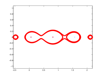
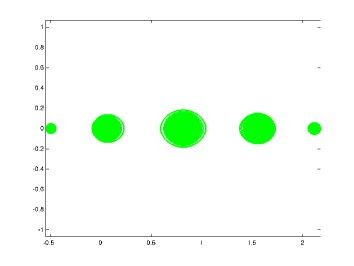
Figure 1: Example 1. Left plot: $\Lambda_{\varepsilon_{1}}(A)$ is approximated by the eigenvalues of matrices of the form $A+\varepsilon_{1}W_{2}$ and $A+\varepsilon_{1}W_{3}$, where the $W_{j}$ are Wilkinson perturbations associated with the eigenvalues $\lambda_{j}$, $j=2,3$ (marked by red squares), for $\eta:=\mathrm{e}^{\mathrm{i}\theta_{k}}$, $\theta_{k}:=2\pi(k-1)/10^{3}$, $k=1:10^{3}$, and $\varepsilon_{1}=10^{-3.2}$. Right plot: $\Lambda_{\varepsilon_{1}}(A)$ approximated by the eigenvalues of matrices of the form $A+\varepsilon_{1}\mathrm{e}^{\mathrm{i}\theta_{k}}E_{i}$, $i,k=1:10^{3}$, where the $E_{i}$ are unit-norm rank-one random perturbations.

Figure 2: Example 1: $\varepsilon$-pseudospectra by Eigtool, where $\varepsilon=10^{k}$, $k=-3.4:0.2:-2.6$. dim shows the order of the matrix.

The estimate (4.1) of the (unstructured) distance from defectivity $\varepsilon_{*}$ is $\varepsilon_{1}=10^{-3.2}$. It is achieved for the indices $2$ and $3$ of the most $\Lambda_{\varepsilon}$-sensitive pair of eigenvalues. Figure 1 (left) displays the spectrum of matrices of the form $A+\varepsilon_{1}W_{2}$ and $A+\varepsilon_{1}W_{3}$, where the $W_{j}$ are Wilkinson perturbations (2.1) associated with the eigenvalues $\lambda_{j}$, $j=2,3$, for $\eta:=\mathrm{e}^{\mathrm{i}\theta_{k}}$ and $\theta_{k}:=2\pi(k-1)/10^{3}$, $k=1:10^{3}$. Here and throughout this section $\eta$ is the leading coefficient of the Wilkinson perturbation (2.1). Details of the computations are described by Algorithm 1.

Data: matrix $A$, eigensystem $\{\lambda_{i},x_{i},y_{i},\;\forall i=1:n\}$

Result: approximated $\Lambda_{\varepsilon}(A)$

1compute $\varepsilon$, $\{\hat{\imath},\hat{\jmath}\}$ by (4.1)

2 compute $W_{\hat{\imath}}:=\varepsilon\,y_{\hat{\imath}}x_{\hat{\imath}}^{H}$, $W_{\hat{\jmath}}:=\varepsilon\,y_{\hat{\jmath}}x_{\hat{\jmath}}^{H}$

3 display the spectrum of $A+\eta W_{\hat{\imath}}$ for $\eta:=\mathrm{e}^{\mathrm{i}\theta_{k}}$, $\theta_{k}=2\pi(k-1)/10^{3}$, $k=1:10^{3}$

4 display the spectrum of $A+\eta W_{\hat{\jmath}}$ for $\eta:=\mathrm{e}^{\mathrm{i}\theta_{k}}$, $\theta_{k}=2\pi(k-1)/10^{3}$, $k=1:10^{3}$

Algorithm 1 Algorithm for computing an approximated pseudospectrum

Figure 1 (right) displays the approximated $\varepsilon_{1}$-pseudospectrum given by the spectra of matrices of the form $A+\varepsilon_{1}\mathrm{e}^{\mathrm{i}\theta_{k}}E_{i}$, $i,k=1:10^{3}$, where the $\theta_{k}$ are defined as above and the $E_{i}$ are random rank-one perturbations with $\|E_{i}\|_{F}=1$. Thus, the figure shows spectra of $10^{6}$ matrices. Figure 2 displays pseudospectra determined by Eigtool [24]. Comparing the $\varepsilon_{1}$-pseudospectrum of Figure 2 with Figure 1 illustrates the effectiveness of the simple approach proposed in this paper. In particular, the approximated $\varepsilon_{1}$-pseudospectrum of Figure 1 (left) provides a much better approximation of the $\varepsilon_{1}$-pseudospectrum than the approximated $\varepsilon_{1}$-pseudospectrum of Figure 1 (right) and requires the computation of many fewer spectra ($10^{3}$ versus $10^{6}$). This makes our approach considerably faster.

We remark that Eigtool uses the spectral norm $\|\cdot\|$ in (1.1), while we apply the Frobenius norm for the matrices $E_{i}$. Since the $E_{i}$ are of rank one, they have the same spectral and Frobenius norms.

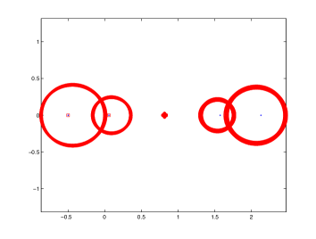
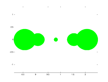
Figure 3: Example 1. Left plot: $\Lambda^{{\mathcal{T}}}_{\varepsilon_{2}}(A)$ is approximated by the eigenvalues of matrices of the form $A+\varepsilon_{2}W^{{\mathcal{T}}}_{1}$ and $A+\varepsilon_{2}W^{{\mathcal{T}}}_{2}$, where the $W^{{\mathcal{T}}}_{j}=W_{j}|_{\widehat{{\mathcal{T}}}}$ are normalized projected Wilkinson perturbations onto ${{\mathcal{T}}}$ associated with the eigenvalues $\lambda_{j}$, $j=1,2$ (marked by red squares), for $\eta:=\mathrm{e}^{\mathrm{i}\theta_{k}}$ and $\theta_{k}:=2\pi(k-1)/10^{3}$, $k=1:10^{3}$, and $\varepsilon_{2}=10^{-0.8}$. Right plot: $\Lambda^{{\mathcal{T}}}_{\varepsilon_{2}}(A)$ is approximated by the eigenvalues of matrices of the form $A+\varepsilon_{2}\mathrm{e}^{\mathrm{i}\theta_{k}}E^{{\mathcal{T}}}_{i}$, $i,k=1:10^{3}$, where the $E^{{\mathcal{T}}}_{i}$ are unit-norm projected random perturbations in ${{\mathcal{T}}}$.

Next we turn to structured pseudospectra and perturbations. Let ${{\mathcal{T}}}$ be the space of tridiagonal Toeplitz matrices of order $5$. We obtain from (4.2) the estimate $\varepsilon_{2}=10^{-0.8}$ of the structured distance from defectivity $\varepsilon^{{\mathcal{T}}}_{*}$. It is achieved for the eigenvalues $\lambda_{1}$ and $\lambda_{2}$. Figure 3 (left) displays the spectra of matrices of the form $A+\varepsilon_{2}W^{{\mathcal{T}}}_{1}$ and $A+\varepsilon_{2}W^{{\mathcal{T}}}_{2}$, where $W^{{\mathcal{T}}}_{1}=W_{1}|_{\widehat{{\mathcal{T}}}}$ and $W^{{\mathcal{T}}}_{2}=W_{2}|_{\widehat{{\mathcal{T}}}}$ are normalized projected Wilkinson perturbations onto ${{\mathcal{T}}}$ associated with the eigenvalues $\lambda_{1}$ and $\lambda_{2}$, respectively, for $\eta:=\mathrm{e}^{\mathrm{i}\theta_{k}}$ and $\theta_{k}:=2\pi(k-1)/10^{3}$, $k=1:10^{3}$. The computations are described by Algorithm 2 with ${\cal S}={\cal T}$.

Data: matrix $A$, eigensystem $\{\lambda_{i},x_{i},y_{i},\;\forall i=1:n\}$

Result: approximated $\Lambda_{\varepsilon^{{\mathcal{S}}}}^{{\mathcal{S}}}(A)$

1compute $\varepsilon^{{\mathcal{S}}}$, $\{\hat{\imath},\hat{\jmath}\}$ by (4.2)

2 compute $W^{{\mathcal{S}}}_{\hat{\imath}}:=\varepsilon^{{\mathcal{S}}}\,y_{\hat{\imath}}x_{\hat{\imath}}^{H}|_{\widehat{{\mathcal{S}}}}$, $W^{{\mathcal{S}}}_{\hat{\jmath}}:=\varepsilon^{{\mathcal{S}}}\,y_{\hat{\jmath}}x_{\hat{\jmath}}^{H}|_{\widehat{{\mathcal{S}}}}$

3 display the spectrum of $A+\eta W^{{\mathcal{S}}}_{\hat{\imath}}$ for $\eta:=\mathrm{e}^{\mathrm{i}\theta_{k}}$, $\theta_{k}=2\pi(k-1)/10^{3}$, $k=1:10^{3}$

4 display the spectrum of $A+\eta W^{{\mathcal{S}}}_{\hat{\jmath}}$ for $\eta:=\mathrm{e}^{\mathrm{i}\theta_{k}}$, $\theta_{k}=2\pi(k-1)/10^{3}$, $k=1:10^{3}$

Algorithm 2 Algorithm for computing an approximated structured pseudospectrum

Figure 3 (right) displays an approximation of $\Lambda^{{\mathcal{T}}}_{\varepsilon_{2}}(A)$ given by the spectra of the matrices $A+\varepsilon_{2}\mathrm{e}^{\mathrm{i}\theta_{k}}E^{{\mathcal{T}}}_{i}$, $i,k=1:10^{3}$, where the $E^{{\mathcal{T}}}_{i}$ are random tridiagonal Toeplitz matrices scaled so that $\|E^{{\mathcal{T}}}_{i}\|_{F}=1$. Eigtool [24] cannot be applied to determine structured pseudospectra. Notice that one component of the most $\Lambda_{\varepsilon_{2}}^{{\mathcal{T}}}$-sensitive pair of eigenvalues, $\lambda_{2}$, does not have one of the two largest structured condition numbers; see Table 1. $\blacksquare$

$i$	$\lambda_{i}$	$\kappa(\lambda_{i})$	$\kappa^{{\mathcal{T}}}(\lambda_{i})$
${\phantom{0}}1$	${\phantom{0}}5.4616+6.5356\,\mathrm{i}$	$1.039\cdot 10^{1}$	${\phantom{0}}1.169\cdot 10^{-1}$
${\phantom{0}}2$	${\phantom{0}}3.8552+5.1268\,\mathrm{i}$	$2.999\cdot 10^{1}$	${\phantom{0}}8.646\cdot 10^{-1}$
${\phantom{0}}3$	${\phantom{0}}1.7072+3.1264\,\mathrm{i}$	$5.643\cdot 10^{1}$	${\phantom{0}}5.665\cdot 10^{-1}$
${\phantom{0}}4$	$-3.9451-0.1224\,\mathrm{i}$	$1.534\cdot 10^{1}$	$1.250\cdot 10^{0}$
${\phantom{0}}5$	$-0.7339-3.2688\,\mathrm{i}$	$2.528\cdot 10^{0}$	${\phantom{0}}8.553\cdot 10^{-1}$
${\phantom{0}}6$	${\phantom{0}}0.3809-2.2234\,\mathrm{i}$	$4.908\cdot 10^{0}$	${\phantom{0}}6.596\cdot 10^{-1}$
${\phantom{0}}7$	${\phantom{0}}2.4409-0.7300\,\mathrm{i}$	$2.373\cdot 10^{0}$	${\phantom{0}}8.623\cdot 10^{-1}$
${\phantom{0}}8$	${\phantom{0}}1.5110-1.0247\,\mathrm{i}$	$8.071\cdot 10^{0}$	${\phantom{0}}7.491\cdot 10^{-1}$
${\phantom{0}}9$	$-2.2354+0.4417\,\mathrm{i}$	$5.207\cdot 10^{1}$	${\phantom{0}}9.748\cdot 10^{-1}$
$10$	$-0.2952+1.1966\,\mathrm{i}$	$7.775\cdot 10^{1}$	${\phantom{0}}3.750\cdot 10^{-1}$

Table 2: Example 2: Eigenvalue condition numbers.

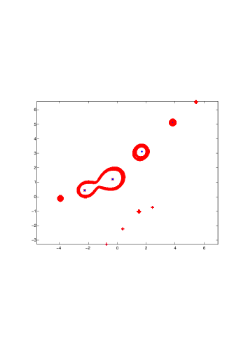
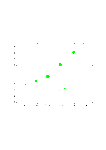
Figure 4: Example 2. Left plot: $\Lambda_{\varepsilon_{1}}(A)$ is approximated by the eigenvalues of matrices of the form $A+\varepsilon_{1}W_{9}$ and $A+\varepsilon_{1}W_{10}$, where the $W_{j}$ are Wilkinson perturbations associated with the eigenvalues $\lambda_{j}$, $j=9,10$ (marked by red squares), for $\eta:=\mathrm{e}^{\mathrm{i}\theta_{k}}$, $\theta_{k}:=2\pi(k-1)/10^{3}$, $k=1:10^{3}$, and $\varepsilon_{1}=10^{-2}$. Right plot: $\Lambda_{\varepsilon_{1}}(A)$ is approximated by the eigenvalues of matrices of the form $A+\varepsilon_{1}\mathrm{e}^{\mathrm{i}\theta_{k}}E_{i}$, $i,k=1:10^{3}$, where the $E_{i}$ are unit-norm rank-one random perturbations.

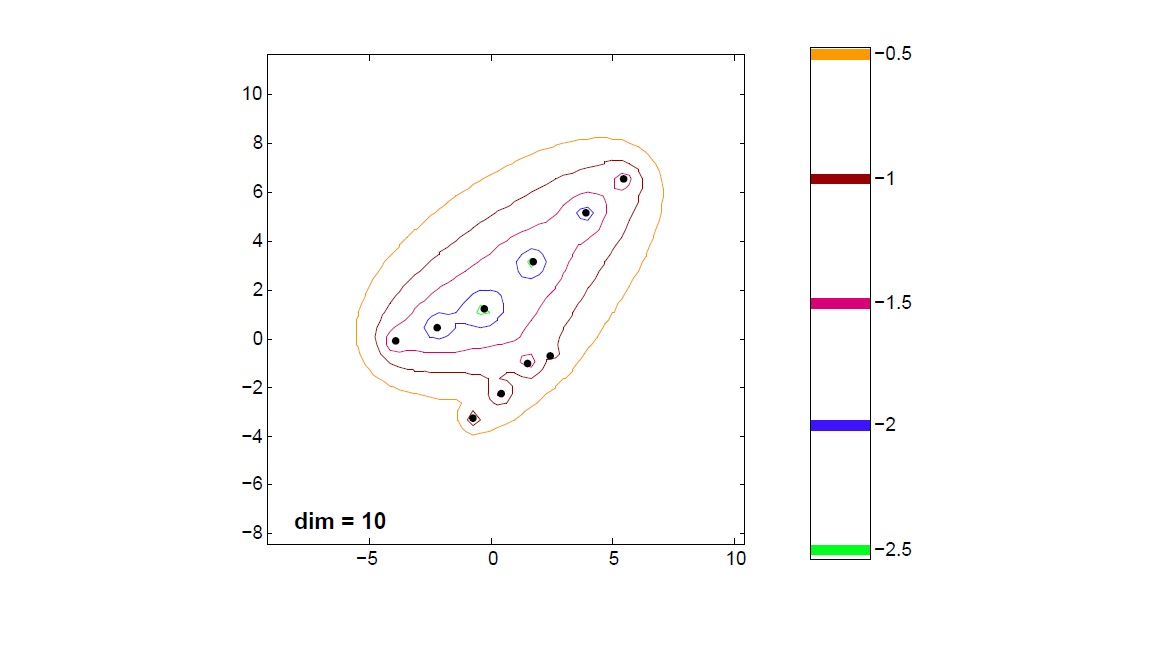
Figure 5: Example 2: $\varepsilon$-pseudospectra by Eigtool, where $\varepsilon=10^{k}$, $k=-2.5:0.5:-0.5$. dim shows the order of the matrix.

Example 2. We consider a complex pentadiagonal Toeplitz matrix of order $n=10$ constructed analogously as the matrix of Example 1. Traditional and structured condition numbers for the eigenvalues are shown in Table 2. The estimate (4.1) of the distance to defectivity is $\varepsilon_{1}=10^{-2}$; it is achieved for the indices $9$ and $10$. Figure 4 (left) displays the spectra of matrices of the form $A+\varepsilon_{1}W_{9}$ and $A+\varepsilon_{1}W_{10}$, where the $W_{j}$ are Wilkinson perturbations (2.1) associated with the eigenvalues $\lambda_{j}$, $j=9,10$, for $\eta:=\mathrm{e}^{\mathrm{i}\theta_{k}}$ and $\theta_{k}:=2\pi(k-1)/10^{3}$, $k=1:10^{3}$. Figure 4 (right) displays the approximated $\varepsilon_{1}$-pseudospectrum given by the spectra of the matrices $A+\varepsilon_{1}\mathrm{e}^{\mathrm{i}\theta_{k}}E_{i}$, $i,k=1:10^{3}$, where the $E_{i}$ are random rank-one perturbations with $\|E_{i}\|_{F}=1$. Figure 5 depicts pseudospectra determined by Eigtool [24]. Comparing the $\varepsilon_{1}$-pseudospectrum of Figure 5 with Figure 4 shows that the simple computations of this paper, based on Wilkinson perturbations (2.1) and illustrated by Figure 4 (left), can give more accurate approximations of pseudospectra and require less computational effort than the approach used for Figure 4 (right). Notice that the most $\Lambda_{\varepsilon_{1}}$-sensitive pair of eigenvalues do not have the largest (unstructured) condition numbers; see Table 2.

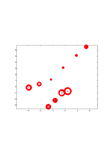
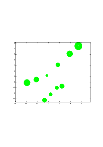
Figure 6: Example 2. Left plot: $\Lambda^{{\mathcal{T}}}_{\varepsilon_{2}}(A)$ is approximated by the eigenvalues of matrices of the form $A+\varepsilon_{2}W^{{\mathcal{T}}}_{7}$ and $A+\varepsilon_{2}W^{{\mathcal{T}}}_{8}$, where the $W^{{\mathcal{T}}}_{j}=W_{j}|_{\widehat{{\mathcal{T}}}}$ are normalized projected Wilkinson perturbations onto ${{\mathcal{T}}}$ associated with the eigenvalues $\lambda_{j}$, $j=7,8$ (marked by red squares), for $\eta:=\mathrm{e}^{\mathrm{i}\theta_{k}}$ and $\theta_{k}:=2\pi(k-1)/10^{3}$, $k=1:10^{3}$, and $\varepsilon_{2}=10^{-0.2}$. Right plot: $\Lambda^{{\mathcal{T}}}_{\varepsilon_{2}}(A)$ is approximated by the eigenvalues of matrices of the form $A+\varepsilon_{2}\mathrm{e}^{\mathrm{i}\theta_{k}}E^{{\mathcal{T}}}_{i}$, $i,k=1:10^{3}$, where the $E^{{\mathcal{T}}}_{i}$ are unit-norm pentadiagonal Toeplitz random perturbations.

We now consider structured perturbations and pseudospectra. Let ${{\mathcal{T}}}$ be the space of pentadiagonal Toeplitz matrices of order $10$. We obtain from (4.2) the estimate $\varepsilon_{2}=10^{-0.2}$ of the structured distance from defectivity $\varepsilon^{{\mathcal{T}}}_{*}$. It is achieved for the eigenvalues $\lambda_{7}$ and $\lambda_{8}$. Figure 6 (left) displays the spectra of matrices of the form $A+\varepsilon_{2}W^{{\mathcal{T}}}_{7}$ and $A+\varepsilon_{2}W^{{\mathcal{T}}}_{8}$, where the $W^{{\mathcal{T}}}_{j}=W_{j}|_{\widehat{{\mathcal{T}}}}$ are normalized projected Wilkinson perturbations onto ${{\mathcal{T}}}$ associated with the eigenvalues $\lambda_{j}$ for $j=7,8$ with $\eta:=\mathrm{e}^{\mathrm{i}\theta_{k}}$ for $\theta_{k}=2\pi(k-1)/10^{3}$, $k=1:10^{3}$. Figure 6 (right) displays the approximation of $\Lambda^{{\mathcal{T}}}_{\varepsilon_{2}}(A)$ given by the spectra of the matrices $A+\varepsilon_{2}\mathrm{e}^{\mathrm{i}\theta_{k}}E^{{\mathcal{T}}}_{i}$, $i,k=1:10^{3}$, where the $E^{{\mathcal{T}}}_{i}$ are random pentadiagonal Toeplitz matrices scaled so that $\|E^{{\mathcal{T}}}_{i}\|_{F}=1$. According to Table 2, the most $\Lambda_{\varepsilon_{2}}^{{\mathcal{T}}}$-sensitive pair of eigenvalues do not have the largest structured condition numbers. $\blacksquare$

$i$	$\lambda_{i}$	$\kappa(\lambda_{i})$	$\kappa^{{\mathcal{H}}}(\lambda_{i})$
$1$	$-2.0595$	$1.092\cdot 10^{0}$	${\phantom{0}}7.725\cdot 10^{-1}$
$2$	${\phantom{0}}2.0595$	$1.092\cdot 10^{0}$	${\phantom{0}}7.725\cdot 10^{-1}$
$3$	$-0.6686$	$1.758\cdot 10^{0}$	$1.252\cdot 10^{0}$
$4$	${\phantom{0}}0.6686$	$1.758\cdot 10^{0}$	$1.252\cdot 10^{0}$
$5$	${\phantom{0}}0.3677$	$4.097\cdot 10^{0}$	$2.926\cdot 10^{0}$
$6$	${\phantom{0}}0.2151$	$3.958\cdot 10^{0}$	$3.009\cdot 10^{0}$
$7$	$-0.2151$	$3.958\cdot 10^{0}$	$3.009\cdot 10^{0}$
$8$	$-0.3677$	$4.097\cdot 10^{0}$	$2.926\cdot 10^{0}$

Table 3: Example 3: Eigenvalue condition numbers.

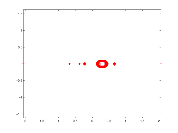
Figure 7: Example 3. Left plot: $\Lambda_{\varepsilon_{1}}(A)$ is approximated by the eigenvalues of matrices of the form $A+\varepsilon_{1}W_{5}$ and $A+\varepsilon_{1}W_{6}$, where the $W_{j}$ are Wilkinson perturbations associated with the eigenvalues $\lambda_{j}$, $j=5,6$ (marked by red squares), for $\eta:=\mathrm{e}^{\mathrm{i}\theta_{k}}$, $\theta_{k}:=2\pi(k-1)/10^{3}$, $k=1:10^{3}$, and $\varepsilon_{1}=10^{-1.6}$. Right plot: $\Lambda_{\varepsilon_{1}}(A)$ is approximated by the eigenvalues of $A+\varepsilon_{1}\mathrm{e}^{\mathrm{i}\theta_{k}}E_{i}$, $i,k=1:10^{3}$, where the $E_{i}$ are unit-norm rank-one random perturbations.

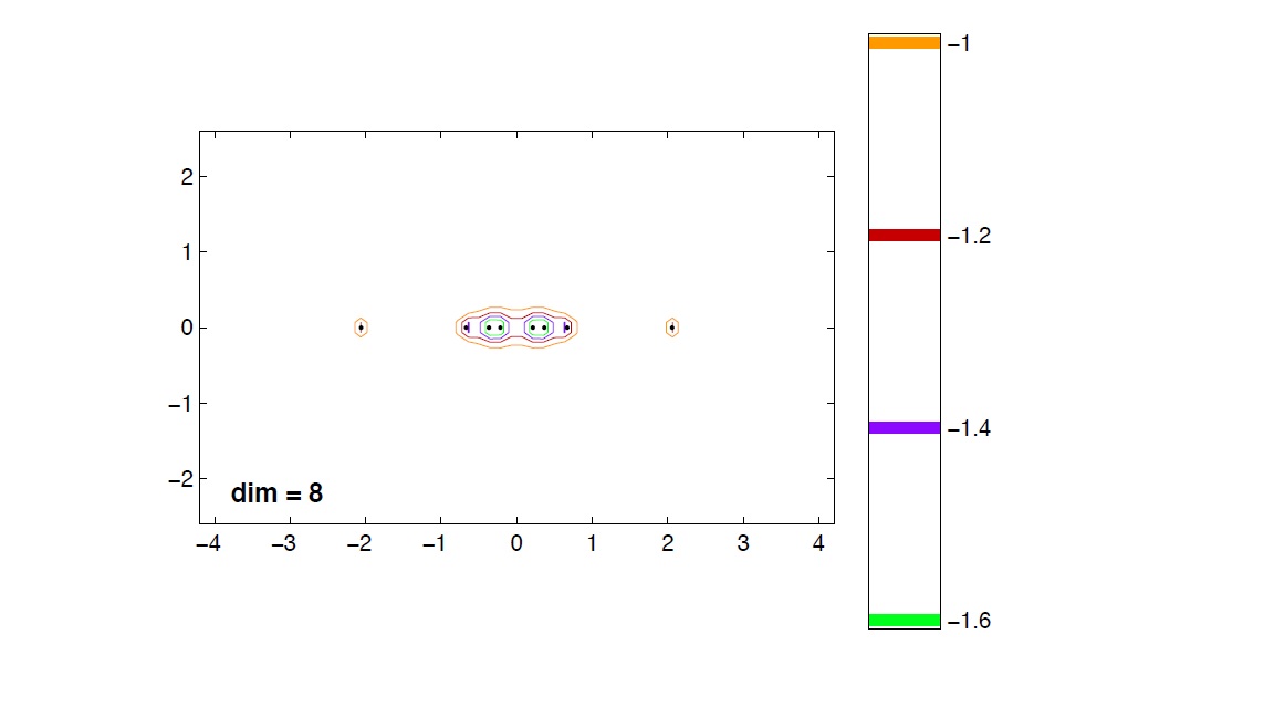
Figure 8: Example 3: $\varepsilon$-pseudospectra by Eigtool, where $\varepsilon=10^{k}$, $k=-1.6:0.2:-1$. dim shows the order of the matrix.

5.2 Hamiltonian structure

Example 3. Let $A=M|_{{{\mathcal{H}}}}$, where $M\in\mathbb{R}^{8\times 8}$ has random entries, i.e., $A$ is the closest Hamiltonian matrix to $M$; cf. Proposition 3.2. The traditional and structured condition numbers for the eigenvalues of $A$ are shown in Table 3. We obtain from (4.1) the upper bound $\varepsilon_{1}=10^{-1.6}$ for the distance to defectivity $\varepsilon_{*}$. It is achieved for the indices $5$ and $6$. Figure 7 (left) is analogous to Figure 4; it displays the spectra of matrices of the form $A+\varepsilon_{1}W_{5}$ and $A+\varepsilon_{1}W_{6}$, where the $W_{j}$ are Wilkinson perturbations (2.1) associated with the eigenvalues $\lambda_{j}$, $j=5,6$, for $\eta:=\mathrm{e}^{\mathrm{i}\theta_{k}}$, $\theta_{k}:=2\pi(k-1)/10^{3}$, $k=1:10^{3}$. Figure 7 (right) shows the approximated $\varepsilon_{1}$-pseudospectrum given by the spectra of the matrices $A+\varepsilon_{1}\mathrm{e}^{\mathrm{i}\theta_{k}}E_{i}$, $i,k=1:10^{3}$, where the $E_{i}$ are random rank-one perturbations with $\|E_{i}\|_{F}=1$. Figure 8 displays graphs produced by Eigtool [24]. A comparison of Figures 7 and 8 shows the effectiveness of using (4.1) to identify pertinent eigenvalue pairs. Similarly as in the preceding examples, $2\cdot 10^{3}$ Wilkinson perturbations yield a much better approximation of the $\varepsilon_{1}$-pseudospectrum than a simulation with $1\cdot 10^{6}$ Hamiltonian random perturbations. The latter simulation does not show coalescence of components of the $\varepsilon_{1}$-pseudospectrum.

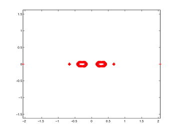
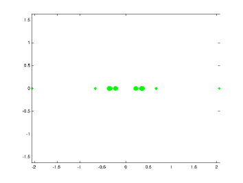
Figure 9: Example 3. Left plot: $\Lambda^{{\mathcal{H}}}_{\varepsilon_{2}}(A)$ is approximated by the eigenvalues of matrices of the form $A+\varepsilon_{2}W^{{\mathcal{H}}}_{5}$ and $A+\varepsilon_{2}W^{{\mathcal{H}}}_{6}$, where the $W^{{\mathcal{T}}}_{j}=W_{j}|_{\widehat{{\mathcal{T}}}}$ are normalized projected Wilkinson perturbations onto ${{\mathcal{H}}}$ associated with the eigenvalues $\lambda_{j}$, $j=5,6$ (marked by red squares), for $\eta:=\mathrm{e}^{\mathrm{i}\theta_{k}}$, $\theta_{k}:=2\pi(k-1)/10^{3}$, $k=1:10^{3}$, and $\varepsilon_{2}=10^{-1.6}$. Right plot: $\Lambda^{{\mathcal{H}}}_{\varepsilon_{2}}(A)$ is approximated by the eigenvalues of $A+\varepsilon_{2}\mathrm{e}^{\mathrm{i}\theta_{k}}E^{{\mathcal{H}}}_{i}$, $i,k=1:10^{3}$, where the $E^{{\mathcal{H}}}_{i}$ are unit-norm Hamiltonian random perturbations.

We now consider structured perturbations and evaluate (4.2). This gives $\varepsilon_{2}=10^{-1.6}$, which is the same as $\varepsilon_{1}$ above. We obtain the same indices, $5$ and $6$, as for the unstructured situation. Figure 9 is analogous to Figure 4. Thus, Figure 9 (left) displays spectra of matrices of the form $A+\varepsilon_{2}W^{{\mathcal{H}}}_{5}$ and $A+\varepsilon_{2}W^{{\mathcal{H}}}_{6}$, where the $W^{{\mathcal{H}}}_{j}=W_{j}|_{\widehat{{\mathcal{H}}}}$ are normalized projected Wilkinson perturbations onto the space ${{\mathcal{H}}}$ of the real Hamiltonian matrices associated with the eigenvalues $\lambda_{j}$, $j=5,6$, with $\eta:=\mathrm{e}^{\mathrm{i}\theta_{k}}$, $\theta_{k}:=2\pi(k-1)/10^{3}$, $k=1:10^{3}$. It is shown in [7] that in this case, the real worst-case perturbations are rank-2 matrices. In fact, one has that just the perturbation $\varepsilon_{2}W^{{\mathcal{H}}}_{5}$ with $\eta=-1$, or even just the perturbation $\varepsilon_{2}W^{{\mathcal{H}}}_{6}$ with $\eta=1$, suffices to cause coalescence of the pairs $(\lambda_{7},\lambda_{8})$ and $(\lambda_{5},\lambda_{6})$; see (3.3). Figure 9 (right) shows an approximation of the spectrum $\Lambda_{\varepsilon_{2}}^{{\mathcal{H}}}(A)$ determined by the spectra of the matrices $A+\varepsilon_{2}\mathrm{e}^{\mathrm{i}\theta_{k}}E^{{\mathcal{H}}}_{i}$, $i,k=1:10^{3}$, where the $E^{{\mathcal{H}}}_{i}$ are Hamiltonian random perturbations scaled so that $\|E^{{\mathcal{H}}}_{i}\|_{F}=1$.

We observe that for both the structured and unstructured cases, the use of (4.1) together with Wilkinson perturbations, or of (4.2) with projected Wilkinson perturbations, give more accurate approximations of the $\varepsilon_{1}$-pseudospectrum and the structured $\varepsilon_{2}$-pseudospectrum, respectively, than using many more unstructured or structured random perturbations. Moreover, the random perturbations do not provide information about coalescence of components of the unstructured or structured pseudospectra.

Note that, although the most $\Lambda_{\varepsilon_{1}}$-sensitive pair of eigenvalues coincide with the most $\Lambda_{\varepsilon_{2}}^{{\mathcal{H}}}$-sensitive pair of eigenvalues, see Table 3, the structured approach has the advantage of preserving eigenvalue symmetries in finite precision arithmetic, as it illustrated by left-hand side plots in Figures 7 and 9.

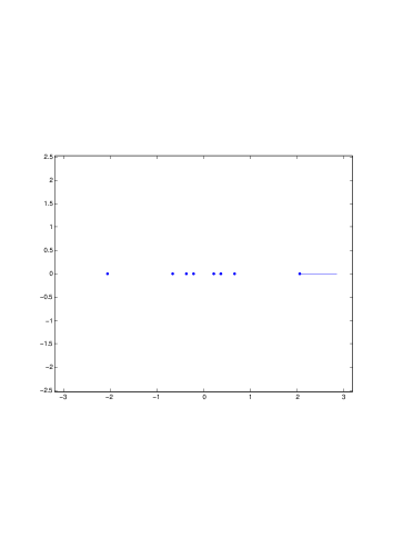
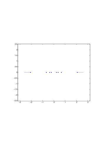
Figure 10: Example 3: Approximated pseudo-eigenvalues and structured pseudo-eigenvalues. Left plot: $E$ has entries $1/n$ and $\varepsilon$ increases from $0$ to $10^{-0.1}$. Right plot: perturbation $E|_{\widehat{{\mathcal{H}}}}$ and the same $\varepsilon$.

We conclude this example with another illustration of the sensitivity of the eigenvalues of $A$ to perturbations. Let $E$ be a rank-one matrix of norm one. Figure 10 shows for all eigenvalues $\lambda_{i}=\lambda_{i}(0)$, $1\leq i\leq 8$, of $A$, the behavior of the pseudo-eigenvalues $\lambda_{i}(\varepsilon)$ of $A+\varepsilon E$ and of the structured pseudo-eigenvalues $\lambda_{i}^{{\mathcal{H}}}(\varepsilon)$ of $A+\varepsilon E^{{\mathcal{H}}}$, where

$$\lambda_{i}(\varepsilon)\approx\lambda_{i}(0)+\varepsilon\frac{y_{i}^{H}Ex_{i}}{y_{i}^{H}x_{i}},\qquad\lambda_{i}^{{\mathcal{H}}}(\varepsilon)\approx\lambda_{i}(0)+\varepsilon\frac{y_{i}^{H}E^{{\mathcal{H}}}x_{i}}{y_{i}^{H}x_{i}},$$

and $y_{i}^{H}x_{i}$ is real and positive. Here $x_{i}$ and $y_{i}$ are right and left unit eigenvectors associated with the eigenvalue $\lambda_{i}(0)$ and $\varepsilon$ increases from $0$ to $10^{-0.1}$. In Figure 10 (left) the perturbation matrix $E$ is the rank-one perturbation with all elements equal to $1/8$, and in Figure 10 (right) the structured perturbation matrix is $E^{{\mathcal{H}}}=E|_{\widehat{{\mathcal{H}}}}$. Real Hamiltonian matrices have eigenvalues in $\pm$ pairs. This can be seen in Figure 10 (right). Also, the rightmost eigenvalue is perturbed less under the structured perturbation. Rough lower bounds for the $\varepsilon$-pseudospectral abscissa and for its structured version can be easily deduced. $\blacksquare$

6 Conclusions and remarks

The computed examples illustrate that standard (unstructured) pseudospectra can be well approximated by using suitable “worst case” rank-one perturbations of the given matrix, i.e., by using Wilkinson perturbations associated with the two eigenvalues whose pseudospectral components are likely to first coalesce, as determined by (4.1). For structured matrices, such as banded non-Hermitian Toeplitz matrices or Hamiltonian matrices, the structured pseudospectra can be well approximated by using normalized projections of Wilkinson perturbations associated with two eigenvalues whose components in the structured pseudospectra are likely to first coalesce, as determined by (4.2). For the Hamiltonian-structured case, this strategy gives rise to rank-two approximated structured pseudospectra, since the Hamiltonian projection of a Wilkinson perturbation is of rank two. Finally, a simple strategy for approximating the structured $\varepsilon$-pseudospectral abscissa [or radius] (with respect to the Frobenius norm) consists of perturbing the original matrix $A$ by the $\varepsilon$-normalized projected Wilkinson perturbation associated with the rightmost [or largest] eigenvalue. We noticed in computations that one often gets an extremely cheap, though quite rough, lower bound for the structured $\varepsilon$-pseudospectral abscissa by computing the real part of the rightmost eigenvalue of $A$ perturbed by the $\varepsilon$-normalized projected all-ones matrix.

References

• [1] R. Alam and S. Bora, On sensitivity of eigenvalues and eigendecompositions of matrices, Linear Algebra and its Applications, 396 (2005), pp. 273–301.
• [2] R. Alam, S. Bora, R. Byers, and M. L. Overton, Characterization and construction of the nearest defective matrix via coalescence of pseudospectral components, Linear Algebra and its Applications, 435 (2011), pp. 494–513.
• [3] C. Bekas and E. Gallopoulos, Parallel computation of pseudospectra by fast descent, Parallel Computing, 28 (2002), pp. 223–242.
• [4] P. Benner, D. Kressner, and V. Mehrmann, Skew-Hamiltonian and Hamiltonian eigenvalue problems: Theory, algorithms and applications, Z. Drmac, M. Marusic, and Z. Tutek, eds., Proceedings of the Conference on Applied Mathematics and Scientific Computing 2003, Springer, Berlin, 2005, pp. 3–39.
• [5] A. Böttcher, S. Grudsky, and A. Kozak, On the distance of a large Toeplitz band matrix to the nearest singular matrix, in: Toeplitz Matrices and Singular Integral Equations (Pobershau, 2001), Operational Theory Advances and Application, vol. 135, Birkhäuser, Basel, 2002, pp. 101–106.
• [6] J. R. Bunch, The weak and strong stability of algorithms in numerical linear algebra, Linear Algebra and its Applications, 88/89 (1987), pp. 49–66.
• [7] P. Buttà and S. Noschese, Structured maximal perturbations of Hamiltonian eigenvalue problems, Journal of Computational amd Applied Mathematics, 272 (2014), pp. 304–312.
• [8] P. Buttà, N. Guglielmi, and S. Noschese, Computing the structured pseudospectrum of a Toeplitz matrix and its extremal points, SIAM Journal on Matrix Analysis and Applications, 33 (2012), pp. 1300–1319.
• [9] P. Buttà, N. Guglielmi, M. Manetta, and S. Noschese, Differential equations for real-structured defectivity measures, SIAM Journal on Matrix Analysis and Applications, 36 (2015), pp. 523–548.
• [10] J. W. Demmel, A Numerical Analyst’s Jordan Canonical Form, Ph.D. Thesis, University of California at Berkeley, 1983.
• [11] S. Graillat, A note on structured pseudospectra, Journal of Computational and Applied Mathematics, 191 (2006), pp. 68–76.
• [12] D. J. Higham and N. J. Higham, Backward error and condition of structured linear systems, SIAM Jouurnal on Matrix Analysis and Applications, 13 (1992), pp. 162–175.
• [13] M. Karow, Structured pseudospectra and the condition of a nonderogatory eigenvalue, SIAM Journal on Matrix Analysis and Applications, 31 (2010), pp. 2860–2881.
• [14] M. Karow, E. Kokiopoulou, and D. Kressner, On the computation of structured singular values and pseudospectra, Systems and Control Letters, 59 (2010), pp. 122–129.
• [15] M. Karow, D. Kressner, and F. Tisseur, Structured eigenvalue condition numbers, SIAM Journal on Matrix Analysis and Applications, 28 (2006), pp. 1052–1068.
• [16] D. Mezher and B. Philippe, Parallel computation of pseudospectra of large sparse matrices, Parallel Computing, 28 (2002), pp. 199–221.
• [17] S. Noschese and L. Pasquini, Eigenvalue condition numbers: zero-structured versus traditional, Journal of Computational and Applied Mathematics, 185 (2006), pp. 174–189.
• [18] S. Noschese and L. Pasquini, Eigenvalue patterned condition numbers: Toeplitz and Hankel cases, Journal of Computational and Applied Mathematics, 206 (2007), pp. 615–624.
• [19] S. Noschese, L. Pasquini, and L. Reichel, Tridiagonal Toeplitz matrices: properties and novel applications, Numerical Linear Algebra with Applications, 20 (2013), pp. 302–326.
• [20] L. Reichel and L. N. Trefethen, Eigenvalues and pseudo-eigenvalues of Toeplitz matrices, Linear Algebra and its Applications, 162-164 (1992), pp. 153–185.
• [21] S. M. Rump, Eigenvalues, pseudospectrum and structured perturbations, Linear Algebra and its Applications, 413 (2006), pp. 567–593.
• [22] L. N. Trefethen and M. Embree, Spectra and Pseudospectra, Princeton University Press, Princeton, 2005.
• [23] J. H.  Wilkinson, The Algebraic Eigenvalue Problem, Oxford University Press, 1965.
• [24] T. G. Wright, Eigtool: a graphical tool for nonsymmetric eigenproblems. Oxford University Computing Laboratory, http://www.comlab.ox.ac.uk/pseudospectra/eigtool/, 2002.
• [25] T. G. Wright and L. N. Trefethen, Large-scale computation of pseudospectra using ARPACK and eigs, SIAM Journal on Scientific Computing, 23 (2001), pp. 591–605.