myfnsymbols** ††‡‡§§‖∥¶¶
The Probability of Extinction of Infectious Salmon Anemia Virus in One and Two Patches
Abstract.
Single type and multitype branching process have been used to study the dynamics of a variety of stochastic birth-death type phenomena in biology and physics. Their use in epidemiology goes back to Whittle’s study of a Susceptible–Infected–Recovered (SIR) model in the 1950s. In the case of an SIR model, the presence of only one infectious class allows for the use of single type branching processes. Multitype branching processes allow for multiple infectious classes and have latterly been used to study metapopulation models of disease. In this article, we develop a Continuous Time Markov Chain (CTMC) model of Infectious Salmon Anemia virus in two patches, two CTMC models in one patch and companion multitype branching process (MTBP) models. The CTMC models are related to deterministic models which inform the choice of parameters. The probability of extinction is computed for the CTMC via numerical methods and approximated by the MTBP in the supercritical regime. The stochastic models are treated as toy models and the parameter choices are made to highlight regions of the parameter space where CTMC and MTBP agree or disagree, without regard to biological significance. Partial extinction events are defined and their relevance discussed. A case is made for calculating the probability of such events, noting that MTBP’s are not suitable for making these calculations.
Evan Milliken∗
School of Mathematical and Statistical Sciences, Arizona State University
1. Introduction
In the investigation that follows, we will use the case of an outbreak of Infectious Salmon Anemia (ISA) as a test case to examine some of the features of MTBP approximation of a CTMC. Infectious salmon anemia virus (ISAv) causes (ISA) which leads to 15 – 100% accumulated mortality over the course of a several months long infection in a farm environment Falk et al., (1997). It is found in all large salmon-producing countries including Norway, Scotland, Ireland, Canada, the United States, and Chile Vike et al., (2009). ISAv is transmitted among finfish horizontally by passive movement of infected seawater Mardones et al., (2009) and via direct contact with excretions or secretions of infected individuals. Salmon farms consist of a collection of net cages placed in open body of water. This array-like structure of a farm and the proximity of farms to each other and to wild salmon migratory routes justifies the use of a metapopulation approach.
Branching processes have been used to study a variety of biological phenomena dating back to their invention to answer a question regarding the extinction of aristocratic surnames. Bienaymé made the first contribution in 1845 Seneta, (1998) before the question was made well known by Galton and answered together with Watson in 1873-4 Watson and Galton, (1875). As a result, the class of single type branching processes came to be known as Bienaymé–Galton–Watson branching processes (BGWbp). A special case considering two types of individuals was studied by Bartlett in 1946 and BGWbp theory was extended to include general multitype branching processes by Kolmogorov, Dmitriev, Sevastyanov, Everett and Ulam in the late 1940’s Harris, (1963). BGWbp and MTBP models have been used to study a variety of phenomena in biology and physics including population dynamics, changes to the genome, cell kinetics, cancer and epidemiology Allen, (2003); Allen and Lahodny, (2012, 2013); Allen and van den Driessche, (2013); Ball, (1983); Ball and Donnelly, (1995); Britton, (2010); Dorman et al., (2004); Griffiths and Greenhalgh, (2011); Harris, (1963); Kimmel and Axelrod, (2002); Whittle, (1955). In particular, Allen and Lahodny studied MTBP’s as an approximation of the outbreak dynamics of a CTMC model of infection in single and multi-patch models Allen and Lahodny, (2012, 2013).
We recall earlier analysis of deterministic Susceptible-Infected-Virus (SIV) models of ISAv outbreak in one and two patches to inform our investigation and aid in suitable parameter selection Milliken and Pilyugin, (2016). The model in one patch is adapted from well-studied models Beretta and Kuang, (1998); Nowak and May, (2000); Perelson and Nelson, (1999) by allowing for direct transmission via contact with infected individuals. For each of these two models, a companion CTMC model is introduced, as well as a MTBP. The probability of extinction of the disease is approximated for the CTMC using numerical simulation. Approximation is also made via analysis of the MTBP and the results are compared with those of numerical simulation.
Formulation of a birth–death process as a branching process relies on the fact that all transitions are independent Allen and Lahodny, (2012); Harris, (1963); Mode, (1971). This is a strong biological assumption, but one commonly made for the purpose of mathematical modeling. In order to formulate epidemiological models as branching processes, an additional assumption is made: the susceptible population remains fixed at its initial (disease-free) population size. As a result of this assumption, MTBP only provides accurate approximation of the probability of disease extinction when the total population size is sufficiently large. There is currently no analytic estimate for how large is sufficiently large. In order to illustrate the breakdown of MTBP approximation and explore its dependence on the underlying system and its parameters, we calculate the probability of extinction for a one-patch system for a range of initial population sizes at two different levels of infected fish mortality. We also propose a variation on the deterministic one-patch model by changing the assumed force of infection (f.o.i.). Corresponding CTMC and MTBP models are also developed. The probability of extinction is again calculated at various initial population sizes.
MTBP techniques are suitable to calculate the probability of complete extinction of the disease in all forms and in all patches. A partial extinction event is one in which one or more classes of infectious individuals goes extinct, but at least some class remains endemic. Such events are transient from the prospective of deterministic and stochastic modeling and have not been considered to date. Metapopulation models are characterized by multiple patches and the rates of movement between them. It is of particular interest to consider partial extinction events in a metapopulation in which the disease goes extinct in some, but not all patches. Statistics like the probability of partial extinction events may help to understand how the underlying structure of the metapopulation influences the dynamics of the system. Additionally, the probability of extinction in a single patch of a metapopulation model may be viewed as a numerical rating of how susceptible that patch is to outbreak of disease. When a patch corresponds to a locality, this rating could then be used to optimize control strategies from the perspective of that patch. An attempt to study partial extinction events for an outbreak of ISAv in two patches using MTBP techniques led to the determination that these techniques are not suitable to answer such questions.
2. two-patch model of ISAv
We begin by illustrating the use of MTBP to approximate the probability of extinction in metapopulation models by taking a two-patch model of ISAv as a test case. The CTMC is constructed so that it is related to a previously studied deterministic model Milliken and Pilyugin, (2016). As a result, the quasi-steady state is equal to the endemic equilibrium of the deterministic model. Parameters are chosen to ensure the quasi-steady state associated to outbreak exists and can be easily located numerically. They are also chosen to ensure the accuracy of the MTBP approximation. They are not chosen for biological relevance.
2.1. Deterministic SIV-SIV model
In previous work with S. S. Pilyugin Milliken and Pilyugin, (2016), we proposed a two-patch SIV model to study the dynamics of an ISAv infection. The two patches are coupled solely via diffusion of the virus. Birth and death rates are patch dependent and are denoted by a subscript associated to the patch. All other parameters are patch independent. The force of infection in the patch is given by , but the parameters and can be scaled away. Rescaling yields the following system:
| (1) |
where are the patch specific birth rates of susceptible fish, are the patch specific, density dependent mortality rates, is the mortality rate of infected fish, is the rate at which infected fish shed the virus into the environment, is the rate at which it clears from the environment and is the rate of viral diffusion.
System (1) admits 7 equilibria in total. Four equilibria corresponding to the absence of the virus: (0,0,0,0,0,0), , , DFE . Of these, only the disease-free equilibrium (DFE) is locally stable in the subspace associated to the absence of the disease. Let
Then is the patch specific reproduction numbers corresponding to host fish only in patch . System (1) admits two additional equilibria corresponding to the case where there are host fish only in patch one or only in patch two: and . The basic reproduction number for system (1) is given by
where Following Milliken and Pilyugin, (2016), we have that DFE is globally asymptotically stable (g.a.s.) if and only if . If , then the DFE is unstable and the virus invades and persists when introduced. In fact, the subset of the boundary associated to the extinction of the virus is a uniform strong repeller whenever Butler et al., (1986); Fonda, (1988); Freedman et al., (1994); Garay, (1989); Hofbauer and So, (1989); Milliken and Pilyugin, (2016); Thieme, (1993). If, in addition, the following symmetric conditions are met,
where , then there exists a unique positive endemic equilibrium.
2.2. Stochastic SIV-SIV model
From the preceding deterministic model we construct the CTMC, , with the infinitesimal transition probability to state from state given by
where is the rate associated to the transition from state to state and can be found in Table 1.
| Description | Transition | rate |
|---|---|---|
| Birth of | ||
| Death of | ||
| Infection of | ||
| Death of | ||
| Shedding of | ||
| Clearance of | ||
| Diffusion of | ||
| Birth of | ||
| Death of | ||
| Infection of | ||
| Death of | ||
| Shedding of | ||
| Clearance of | ||
| Diffusion of |
Remark 1.
Recall that the original force of infection in the patch given by . and are rescaled and and relabeled yielding (1) for easier analysis. The that is retained represents a scalar multiple of the number of virions present. Let and reflect and chosen so that we may interpret 1 unit of as any number of virions, such as an average infectious viral dose (e.g. ID50). This makes the transition in the rescaled model reasonable.
We are interested in studying the dynamics after infectious agents are introduced to an entirely susceptible system. Analysis of the flow of (1) on the boundary shows that, in absence of the disease, DFE is g.a.s.. Therefore, we assume that DFE is the initial state of the system prior to introduction of the disease. As evolves in time, and evolve along with all the other state components. To formulate the MTBP we first pass to embedded discrete time Markov chain (DTMC), . Next, suppose that and , the disease-free populations of susceptible fish in patches 1 and 2, respectively and that each individual gives birth independently of other individuals. Let be the random variable associated to the generation. The offspring probability generating function (pgf) is given by
where, for
and is the probability that an object of type gives birth to offspring of type 1, and offspring of type . The offspring pgf for is
the offspring pgf for is
the offspring pgf for is
and the offspring pgf for is
The matrix of expectations is given by
A branching process is called positively regular if is primitive. A –many type process is called not singular if with respect to the standard order, and whenever with , then . The entry of is , the expected number of type offspring of an individual of type . Following Harris Harris, (1963), let be the extinction probability if initially there is one object of type , . Let . Let be the probability of extinction of the branching process given that . Since we have assumed that individuals give birth independent of one another,
The branching process constructed above to approximate ISAv in two patches is positively regular (in fact, ). It is easily verified that it is also not singular. The Threshold Theorem of Allen and van den Driessche Allen and van den Driessche, (2013) and Theorem 7.1 of Harris Harris, (1963) combine to give the following result.
Theorem 2.1.
Suppose is a MTBP with probability generating function such that , whenever with , and is primitive. If , then . If , then is the unique vector satisfying .
Remark 2.
For a fixed initial vector , the probability of extinction . In a metapopulation model, the probability of extinction is, therefore, the probability that all infectious classes go extinct, in all patches. If we wanted to use MTBP approximation to calculate a partial extinction event, like extinction in one patch, we would have to recast the MTBP to only track the evolution of those infectious classes and assume the number of individuals in other infectious classes remain fixed. However, we already assumed that there are few individuals initially present in each infectious class. As we have discussed above, in order to justify the assumption that the number of individuals in a given class remains fixed, the initial population in that class must be sufficiently large. The MTBP is, therefore, not the appropriate tool to study partial extinction events.
2.3. Numerical example
In order to illustrate the accuracy of MTBP approximation of the probability of total extinction in a metapopulation model, we choose parameter values according to two criteria: the disease-free number of susceptible fish is sufficiently large in each patch for approximation by branching process; and the endemic equilibrium of the deterministic system (1) can be located numerically. The endemic equilibrium of (1) is a quasi-steady state of the CTMC and the embedded DTMC. The second criterion also implies that . Therefore, purely for the purpose of illustration and without regard to biological relevance, we consider the parameter vector . Then , , , , and . Recall that , where and is the extinction probability if there is initial one object of type . Because of this and due to the computational expense of simulating this model, we only consider initial states with one object of type , . The vector of extinction probabilities is determined by iterating the pgf from the initial vector . Let denote the probability of extinction approximated by numerical simulation over realizations. The results are presented in Table 2.
| 1 | 0 | 0 | 0 | 0.0406 | 0.0410 |
| 0 | 1 | 0 | 0 | 0.0501 | 0.0501 |
| 0 | 0 | 1 | 0 | 0.0538 | 0.0542 |
| 0 | 0 | 0 | 1 | 0.0650 | 0.0652 |
By the law of large numbers, as the number of realizations, , increases to infinity, tends to the true probability of extinction. Assuming that is distributed normally, the error in approximating with goes to zero like . This implies that approximation of to three decimal places by numerical simulation requires making realizations, at great computational expense.
The results in Table 2 suggest that the MTBP approximates the probability of extinction in the CTMC very accurately. In this case, we were not able to solve the nonlinear system of equations given by for an analytical solution to the MTBP. However, we are able to approximate by iteration with little computational expense, since .
3. one-patch model
As discussed above, we must assume the number of susceptible individuals remains fixed at the disease-free level in order to utilize branching process techniques for SIV models. The disease-free population size must be at least as large as some critical value in order for this assumption to be reasonable. Currently, there is no analytic estimate of this critical size. In this section and section 5, we compare MTBP approximation and simulation of the CTMC at a range of small initial populations for two models. These models are introduced in this section and the next. The first is an invariant subsystem of (1), which models the dynamics of infection in a single patch. We consider this one-patch model because it reduces the computational expense while still retaining the key features of interest.
3.1. Deterministic SIV model
When there is no diffusion, i.e. , then each patch of the two-patch system forms an invariant SIV subsystem given by:
| (2) |
where , is the birth rate of susceptible fish, the mortality rate of susceptible fish, the mortality rate of infected fish, is the rate of viral clearing and is the rate of viral shedding. All of these parameters are assumed to be positive.
The system admits equilibria (0,0,0) (which is always unstable) and the disease-free equilibrium (DFE), (,0,0). The basic reproduction number is,
| (3) |
When the system also admits a unique positive endemic equilibrium. is also a threshold for the dynamics of the system. If , then the DFE is g.a.s.. If , then the DFE is unstable and the virus invades and persists when introduced. The largest invariant subset of the boundary is a uniform strong repeller when Milliken and Pilyugin, (2016); Thieme, (1993).
3.2. Stochastic SIV model
The CTMC model associated to system (2) with is characterized by the transition rates given in Table 3.
| Description | Transition | rate |
|---|---|---|
| Birth of | ||
| Death of | ||
| Infection | ||
| Death of | ||
| Shedding of | ||
| Clearance of |
To estimate the probability of extinction of the virus, we approximate the CTMC near the DFE. As in the two-patch case, we pass to the embedded DTMC, assume that and that all individuals give birth independently. Let and construct the probability-generating function (pgf) for the MTBP, .
It follows that is not singular and the matrix of expectations is given by
is positive. Thus, is primitive and Theorem 2.1 applies. Solving the system of nonlinear equations given by yields
| (4) |
| (5) |
Then the probability of extinction given that is
Note that, for this model, the MTBP approximation of the probability of extinction can be determined analytically. That is, can be expressed as a continuous function of the parameters.
3.3. Numerical example
For the purpose of illustrating the accuracy of the MTBP approximation, we consider the parameter vector given by . This choice of parameters yields and . Let denote the probability of extinction predicted by the MTBP, given . The probability of extinction in the CTMC is estimated by simulating numerically. Let denote the probability of extinction approximated by numerical simulation over realizations. The results of both approximations are presented in Table 4.
| 1 | 0 | 0.0406 | 0.0407 |
|---|---|---|---|
| 0 | 1 | 0.0495 | 0.0494 |
| 1 | 1 | 0.0020 | 0.0020 |
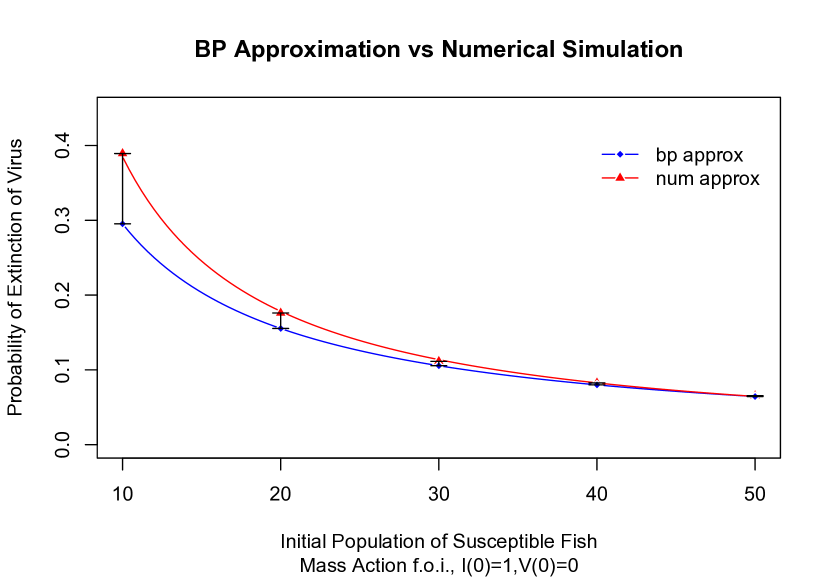
Table 4 illustrates that, for this choice of parameters, the MTBP provides extremely accurate results. Since can be expressed as a function of the parameters, the computational expense for MTBP approximation is negligible. However, we cannot be certain, a priori, whether or not the disease-free population of susceptible fish is sufficiently large without comparing the MTBP results to numerical simulation. Therefore, the estimate of computational expense for MTBP approximation should include the cost of simulating the CTMC. The additional expense for simulating the CTMC can be significant.
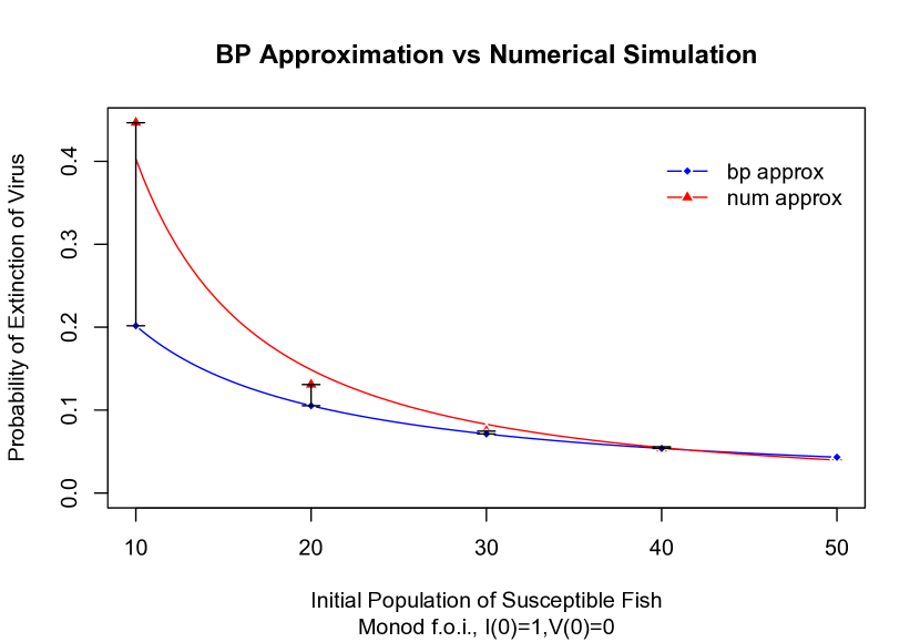
In Figure 2, we compare MTBP and numerical simulation for initial populations at ten unit increments from 10 to 50. First, note that the population of susceptible fish at DFE is given by . Therefore, by assuming , we have that . We fix the remaining parameters and vary from 10 to 50 in ten unit increments.
Numerical data in Figure 2 is fit with a power law curve where and . Not pictured, the absolute error is fit with a power law curve with and and the relative error is fit with a power law curve with and . Since is a continuous function of the parameters, there was no need to fit a curve to the MTBP results.
In Section 5, we will show that the character and speed of convergence of the MTBP approximation results to the CTMC simulation results depends on the structure of the model and the choice of parameters. We do this by constructing illustrations similar to Figure 2 based on variations of the one-patch model.
4. one-patch model with modified force of infection
4.1. Deterministic model
The one-patch model given by system (2) proposes a mass action force of infection. It has been suggested that the f.o.i. may initially be driven by infected salmon encountering susceptible salmon when there are low levels of free virus present at the outset of an exposure event. As more salmon become infected and shed more and more virus into the environment, the free virus may then drive the infection. To account for this we modify system (2) by considering where
Note that when and , the growth function simplifies to the standard Michelis-Menten function for . System (2) with admits equilibria at and the DFE . Following the next generation matrix approach Diekmann et al., (1990); Van Den Driessche and Watmough, (2002) the basic reproduction number is determined to be
| (6) |
The endemic equilibrium is a root of the vector field. From we have . Substituting into yields . Let and . Then the nonnegative root of is a root of the equation
| (7) |
Furthermore, and . Thus, (7) has a unique positive root if and only if . Thus, the unique positive endemic equilibrium exists if and only if . If , then the DFE is g.a.s.. This system has the same dynamics on the boundary as the system with mass action f.o.i.. Using arguments similar to those in Milliken and Pilyugin, (2016), it follows that system (2) with is uniformly strongly persistent whenever Thieme, (1993).
4.2. Stochastic model
The CTMC model related to system (2) with is characterized by the transitions and rates given in Table 5.
| Description | Transition | rate |
|---|---|---|
| Birth of | ||
| Death of | ||
| Infection | ||
| Death of | ||
| Shedding of | ||
| Clearance of |
We approximate the CTMC, , near the DFE with the MTBP, , with the pgf
The matrix of expectations is given by
Clearly, the branching process in not singular and is a positive matrix. Thus, Theorem 2.1 applies. Let , , and
| (8) |
Then ,
| (9) |
| (10) |
Given , can be expressed as a continuous function of the parameters.
4.3. Numerical example
For the purpose of illustrating the accuracy of the MTBP approximation, we consider the parameter vector given by . This implies that and . Let denote the probability of extinction predicted by the MTBP, given . The probability of extinction in the CTMC is estimated by simulating numerically. Let denote the probability of extinction approximated by numerical simulation over realizations. The extinction probability predicted by the branching process approximation is compared with numerical results in Table 6.
| 1 | 0 | 0.0538 | 0.0548 |
|---|---|---|---|
| 0 | 1 | 0.0596 | 0.0606 |
| 1 | 1 | 0.0032 | 0.0042 |
This model represents a variant to the one-patch model studied in Section 3 which differs only in the choice of function for the force of infection.
5. Critical Size of disease-free Population
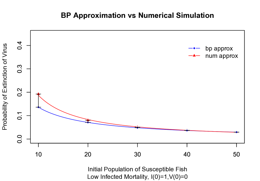
In this section, we illustrate how variations to the underlying model affect the accuracy of MTBP approximation for small initial populations. Figure 2 at the end of Section 3 shows how MTBP approximation diverges from the probability of extinction in the CTMC for small initial populations when . We take this illustration as a baseline and vary the system in two ways. First, we leave , but reduce the mortality rate of infected fish from to . Second, we let as in the baseline, but let as in the model developed in Section 4. In Figure 4, we set and fix the parameter vector with low mortality of infected fish and vary from 10 to 50 in ten unit increments. Numerical data is fit with a power law curve where and . Not pictured, the absolute error is fit with a power law curve with and and the relative error is fit with a power law curve with and .
In Figure 5, we set and fix the parameter vector and vary from 10 to 50 in ten unit increments. Numerical data is fit with a power law curve where and . Not pictured, the absolute error is fit with a power law curve with and and the relative error is fit with a power law curve with and .
Note that the results in Figures 2, 4, and 5 are graphed on the same axes on the same scale. It is immediately evident that the character of convergence of the MTBP varies from the baseline illustration in each of the two latter ones. It is harder to see from the graphs themselves, but the speed of convergence varies slightly as well. This can be seen in Table 7.
| Init. Pop. | |||
|---|---|---|---|
| 10 | 0.094 | 0.056 | 0.245 |
| 20 | 0.021 | 0.009 | 0.025 |
| 30 | 0.006 | 0.003 | 0.003 |
| 40 | 0.003 | 0.001 | 0.002 |
| 50 | 0.001 | 0.000 | 0.001 |
6. Discussion
In this article, we use a model of ISAv in two patches and an invariant subsystem corresponding to one patch as toy models to develop CTMC models and MTBP approximations to estimate the probability of disease outbreak. In addition to these models, we formulate a new one-patch model by varying the force of infection function. In the case of the two-patch model, we approximate the probability of disease extinction, , by iterating the probability generating function of the MTBP. For each one-patch model, characterized by its force of infection, it is possible to write the MTBP approximation of as a continuous function of the parameters. By comparing MTBP results to numerical simulation of the related CTMC, we show that, for large initial populations of susceptible fish, the MTBP approximation provides a good estimate of . However, we should also note that MTBP approximation fails to provide accurate estimates of when the initial population of susceptible fish is low. It is therefore necessary to approximate by numerical simulation concurrent with MTBP approximation. While the computational expense for MTBP approximation is negligible, the computational expense for numerical simulation of the related CTMC, can be very high, especially for metapopulation models.
In this article, we have not provided an analytical estimate on how large the initial population of susceptible individuals needs to be in order for the MTBP approximation to provide a good estimate of . We have, however, illustrated the manner in which the approximation diverges from the true probability in several test cases. Comparison of results in Figures 2, 4, 5 and Table 7 suggest that an analytical estimate will be model specific and parameter dependent.
In Whittle, (1955), Whittle determined that the probability of extinction for a Susceptible-Infected (SI) model was the reciprocal of . This result was also verified by Allen and Lahodny, (2012). Allen and van den Driessche, (2013) showed that and have the same sign, where is the spectral radius of the matrix of first moments, . This implies that efforts that reduce will also increase the probability of extinction. For the models studied in this article, one way to reduce is to decrease the birth rate of susceptible fish, . Unfortunately, this also has the effect of reducing the disease-free equilibrium population size. Never-the-less, in Figures 2, 4 and 5, we see that as is decreased, the probability of extinction increases as measured both by branching process approximation and computer simulation.
Metapopulation models are characterized by their patch structure and the rates of migration between patches. In order to study stochastic metapopulations, it would be useful to study how statistics like probability of extinction vary from patch to patch. In addition, the probability of partial extinction events, like extinction in one patch, may be useful in measuring the effectiveness of control strategies. One would expect it to be especially useful when studying the effectiveness of control strategies that are deployed heterogeneously. Mathematically, the problem of calculating the probability of extinction corresponds to the classical problem of hitting a subspace of the state space of the CTMC from some initial state. In the case of total extinction events, this relates to hitting the subspace of the state space where all infectious classes are zero. Taking the two-patch model (1) as an example, total disease extinction relates to hitting the subspace . However, for partial extinction events, it relates to hitting a subspace of the state space where some infectious classes are zero, but others are positive. For example, extinction in patch one of the two-patch model relates to hitting the subspace . MTBP’s track only the infectious classes and are constructed to calculate the probability of hitting the origin, . As such, MTBP approximation is only suited to calculating the probability of total extinction.
Acknowledgements
This work was conducted with the support from NSF grants DMS-1411853, DMS-1515661 and the Center for Applied Mathematics at University of Florida. The author would like to thank the referees for their helpful suggestions.
References
- Allen, (2003) Allen, L. J. S. (2003). An Introduction to Stochastic Process with Applications to Biology. Pearson/Prentice Hall, Upper Saddle River, NJ.
- Allen and Lahodny, (2012) Allen, L. J. S. and Lahodny, G. E. (2012). Extinction Thresholds in Deterministic and Stochastic Epidemic Models. J. Biol. Dyn., 6(2):590–611.
- Allen and Lahodny, (2013) Allen, L. J. S. and Lahodny, G. E. (2013). Probability of a Disease Outbreak in Stochastic Multipatch Epidemic Models. Bull Math Biol, 75(7):1157–1180.
- Allen and van den Driessche, (2013) Allen, L. J. S. and van den Driessche, P. (2013). Relations Between Deterministic and Stochastic Thresholds for Disease Extinction in Continuous- and Discrete-Time Infectious Disease Models. Math. Biosci., 243(1):99–108.
- Ball, (1983) Ball, F. G. (1983). The Threshold Behaviour of Epidemic Models. J. Appl. Prob., 20(7):227–241.
- Ball and Donnelly, (1995) Ball, F. G. and Donnelly, D. (1995). Strong Approximations for Epidemic Models. Stoch. Proc. Appl., 55(1):1–21.
- Beretta and Kuang, (1998) Beretta, E. and Kuang, Y. (1998). Modeling and Analysis of a Marine Bacteriophage Infection. Math Biosci, 149:57–76.
- Britton, (2010) Britton, T. (2010). Stochastic Epidemic Models: A survey. Math. Biosci., 225:24–35.
- Butler et al., (1986) Butler, G., Freedman, H. I., and Waltman, P. (1986). Uniformly Persistent Systems. Proc. Amer. Math. Soc., 96:425–430.
- Diekmann et al., (1990) Diekmann, O., Heesterbeek, J. A. P., and Metz, J. A. J. (1990). On the Definition and Computation of the Basic Reproduction Ratio R0 in Models of Infectious Disease in Heterogeneous Populations. J. Math. Biol., (28):365–382.
- Dorman et al., (2004) Dorman, K. S., Sinsheimer, J. S., and Lange, K. (2004). In the Garden of Branching Processes. SIAM Rev., 46(2):202–229.
- Falk et al., (1997) Falk, K., Namork, E., Rimstad, E., Mjaaland, S., and Dannevig, B. H. (1997). Characterization of Infectious Salmon Anemia Virus, an Orthomyxo-like Virus Isolated from Atlantic Salmon (Salmo salar L.). J. Virol., 71(12):9016–23.
- Fonda, (1988) Fonda, A. (1988). Uniformly Persistent Semidynamical Systems. Proc. Am. Math. Soc., 104:111–116.
- Freedman et al., (1994) Freedman, H. I., Ruan, S., and Tang, M. (1994). Uniform Persistence and Flows Near a Closed Positively Invariant Set. J. Dyn. Differ. Equations, 6(4):583–600.
- Garay, (1989) Garay, B. (1989). Uniform Persistence and Chain Recurrence. J. Math. Anal. Appl., 139:372–381.
- Griffiths and Greenhalgh, (2011) Griffiths, M. and Greenhalgh, D. (2011). The Probability of Extinction in a Bovine Respiratory Syncytial Virus Epidemic Model. Math. Biosci., 231(2):144–158.
- Harris, (1963) Harris, T. E. (1963). The Theory of Branching Processes. Springer-Verlag, Berlin.
- Hofbauer and So, (1989) Hofbauer, J. and So, J. W.-H. (1989). Uniform Persistence and Repellors for Maps. Proc. Am. Math. Soc., 107(4):1137–1142.
- Kimmel and Axelrod, (2002) Kimmel, M. and Axelrod, D. E. (2002). Branching Processes in Biology. Springer, New York.
- Mardones et al., (2009) Mardones, F. O., Perez, A. M., and Carpenter, T. E. (2009). Epidemiologic Investigation of the Re-emergence of Infectious Salmon Anemia Virus in Chile. Dis. Aquat. Organ., 84(2):105–14.
- Milliken and Pilyugin, (2016) Milliken, E. and Pilyugin, S. S. (2016). A Model of Infectious Salmon Anemia Virus with Viral Diffusion between Wild and Farmed Patches. DCDS-B, accepted.
- Mode, (1971) Mode, C. J. (1971). Multitype Branching Processes Theory and Applications. Elsevier, New York.
- Nowak and May, (2000) Nowak, M. A. and May, R. M. (2000). Virus Dynamics. Oxford University Press, New York.
- Perelson and Nelson, (1999) Perelson, A. S. and Nelson, P. W. (1999). Mathematical Analysis of HIV-I : Dynamics in Vivo. SIAM Rev., 41(1):3–44.
- Seneta, (1998) Seneta, E. (1998). I. J. Bieneymé [1796-1878]: Criticality, Inequality and Internationalization. Int Stat Rev, 66(3):291–301.
- Thieme, (1993) Thieme, H. R. (1993). Persistence Under Relaxed Point Dissipativity (With Applications to an Endemic Model). SIAM J Math Anal, 24(2):407–435.
- Van Den Driessche and Watmough, (2002) Van Den Driessche, P. and Watmough, J. (2002). Reproduction Numbers and Sub-threshold Endemic Equilibria for Compartmental Models of Disease Transmission. Math. Biosci., 180:29–48.
- Vike et al., (2009) Vike, S., Nylund, S., and Nylund, A. (2009). ISA Virus in Chile: Evidence of vertical transmission. Arch. Virol., 154(1):1–8.
- Watson and Galton, (1875) Watson, H. W. and Galton, F. (1875). On the Probability of the Extinction of Families. J. Anthropol. Inst. Gt. Britain Irel., 4:138–144.
- Whittle, (1955) Whittle, P. (1955). The Outcome of a Stochastic Epidemic- A Note on Bailey’s Paper. Biometrika, 42:116–122.