Evaluation of Decentralized Event-Triggered Control Strategies for Cyber-Physical Systems

Abstract

Energy constraint long-range wireless sensor/ actuator based solutions are theoretically the perfect choice to support the next generation of city-scale cyber-physical systems. Traditional systems adopt periodic control which increases network congestion and actuations while burdens the energy consumption. Recent control theory studies overcome these problems by introducing aperiodic strategies, such as event trigger control. In spite of the potential savings, these strategies assume actuator continuous listening while ignoring the sensing energy costs. In this paper, we fill this gap, by enabling sensing and actuator listening duty-cycling and proposing two innovative MAC protocols for three decentralized event trigger control approaches. A laboratory experimental testbed, which emulates a smart water network, was modelled and extended to evaluate the impact of system parameters and the performance of each approach. Experimental results reveal the predominance of the decentralized event-triggered control against the classic periodic control either in terms of communication or actuation by promising significant system lifetime extension.

I Introduction

Over the last decade, there has been a growing trend in industry to transform large-scale manual control and monitoring systems, such as electrical grids and water networks, into fully automatic Cyber-Physical Systems (CPS). The aim of this transformation is the improvement of quality of service and reduction of maintenance cost. In order to achieve these goals, plants and physical environments have been augmented with sensor and actuator nodes which enable monitoring and control by communicating wirelessly and periodically to data centres or local base stations. However, these periodic dynamic control implementations introduce communication and energy consumption overheads.

In large scale CPS, sensor and actuator nodes are usually energy constraint and installed in harsh environments. For example, in smart water network more than 97% of sensing and actuation assets are located underground and powered by batteries [1]. To transmit the required information through long-range (several kilometres) wireless communications, high transmission power is required that leads to fast battery depletion. In addition, the periodic sensing, transmission, and actuation, regardless the state of the plant, decreases network bandwidth and increases actuations and consequently the energy consumption. Recent control theory studies propose to solve these problems by introducing aperiodic strategies, such as Event-Triggered Control (ETC) strategies, e.g. [2, 3, 4, 5, 6, 7] in which the sensors and actuators communicate only when necessary.

In spite of the potential of significant savings, ETC techniques have only been partially examined and implemented on real systems, i.e. [8, 9, 10, 11, 12, 13, 14, 15, 16, 17, 18, 19]. In [10], the authors propose a system based on the Diddyborg robot and examine the strategy presented in [7]. However, this system is first-order and therefore unable to test complex event-triggered strategies. In [19], an experimental evaluation was made for time-triggered control and event-triggered control from [2]. However, this work requires state monitoring continuously to check event conditions. Additionally, the results in [2] can only be used for system with collocated sensors. To the best of our knowledge, there is no experiment that validates and compares different decentralized event-triggered mechanisms under the same conditions.

ETC systems have been studied extensively in order to guarantee convergence of plants under reduced communication schemes. However, the design and implementation of a communication protocol, which fully exploits the ETC behavior and ensures optimal communication, is still missing [20]. State of the art ETC approaches that are focused on communication, i.e. [21, 22, 23, 24, 25, 26, 27, 28, 29],have been limited to simulate or analyze theoretically the impact of network states on system performance. CSMA [30], TDMA [31] and ALOHA [32] were the three communication protocols which have been used in the above approaches. Specifically, [21, 22] provide useful insights and comparison of all the above communication protocols. The authors in [23, 24, 25] present a Markov model that captures the joint interactions of the event-triggering policy and a contention resolution mechanism over CSMA communication. In [26, 27], the ALOHA protocol, which has been applied in Long Term Evolution (LTE) Random Access (RA) procedure, was combined with ETC, with [27] to introduce the impact of collisions into the system performance. TDMA-based communication protocols, i.e. Time Triggered Network-on-a-Chip (TTNoC), Time Triggered Controller Area Network (TTCAN), were analysed in [28], which discusses their application to ETC systems. The earliest practical work is [19], continued in [29], by proposing the extension of the TDMA-based IEEE 802.15.4 MAC layer [33] which has been used in communication protocols for network control via wireless, i.e. WirelessHART [34]. However, the main drawbacks of this approach are the assumption that the actuator nodes listen continuously to network messages. Furthermore, none of the prior work has considered the cost of sensing. For example, in our evaluation platform [35], the sensing costs almost the half the energy consumption of communication. In industrial systems with more energy hungry sensors, e.g. laser based turbidity sensors for water quality, the energy cost may surpass communications.

Uniquely, in this paper, the proposed system duty cycle the sensing and actuator listening activities and at the same time enable decentralized ETC techniques and introducing innovative communication schemes. Specifically, the contributions of this paper are listed as follows:

• Practical combination of sensor duty-cycling with three decentralized aperiodic control approaches.

• A new MAC protocol that facilitates decentralized synchronous ETC without the requirement of continuous actuator communication.

• A novel flexible MAC protocol that can also accommodate two decentralized and asynchronous ETC approaches, communicating firstly absolute states and alternatively relative states only.

By using an extended version of the WaterBox testbed environment [35], we provide experimental results from Time-Triggered Control (TTC) and four different ETC techniques: Periodic centralized ETC (PETC) [4], Periodic Synchronous Decentralized ETC (PSDETC) [5], and Periodic Asynchronous Decentralized ETC (PADETC) by transmitting absolute or relative state [36]. To the best of our knowledge, this is the first real deployment of most of the implemented ETC techniques to a real plant.

II Event-Trigger Control Techniques

We denote the positive real numbers by $\mathbb{R}^{+}$, the natural numbers including zero by $\mathbb{N}$. $|\cdot|$ denotes the Euclidean norm in the appropriate vector space, when applied to a matrix $|\cdot|$ denotes the $l_{2}$ induced matrix norm. A matrix $P\in\mathbb{R}^{n\times n}$ is said to be positive definite, denoted by $P\succ 0$, whenever $x^{\mathrm{T}}Px>0$ for all $x\neq 0$, $x\in\mathbb{R}^{n}$. For the sake of brevity, we write symmetric matrices of the form $\begin{bmatrix}A&B\\ B^{\mathrm{T}}&C\\ \end{bmatrix}$ as $\begin{bmatrix}A&B\\ \star&C\\ \end{bmatrix}$.

II-A Periodic control

Consider a linear time-invariant (LTI) plant and controller

$$\dot{\xi}(t)=A\xi(t)+Bv(t),$$ (1)

$$v(t)=K\xi(t),$$ (2)

where $\xi(t)\in\mathbb{R}^{n}$ is the state vector and $v(t)\in\mathbb{R}^{m}$ is the input vector at time $t$. Assume $A+BK$ is Hurwitz, the system is completely observable, and each sensor can access only one of the system states.

A sample-and-hold mechanism is implemented for the controller (2):

$$v(t)=K\hat{\xi}(t),$$ (3)

where

$$\hat{\xi}(t):=\xi(t_{b}),t\in[t_{b},t_{b+1}[.$$ (4)

and $\{t_{b}\}_{b\in\mathbb{N}}$ is the sequence of the update time of the state. Representing the sample-and-hold effect as a measurement error, we have:

$$\varepsilon(t):=\hat{\xi}(t)-\xi(t).$$ (5)

Define $T$ as the sample period. In a periodic time-triggered control strategy, $t_{b}$ is determined by

$$\{t_{b}|t_{b}=bT,b\in\mathbb{N},T>0\}.$$ (6)

II-B Periodic centralized event-triggered control

In event-triggered control strategies, the control input update time is determined by some pre-designed conditions. These conditions are always a relation between system state and sample-and-hold error (5). Therefore, control executions happen only when necessary. However, the centralized event-triggered condition presented in [2] requires the continuous monitoring and transmission of the current state to check the event conditions. If the state cannot be measured continuously, we can either compute a stricter event condition considering measurement delays; or apply the PETC strategy from [4], which combines periodic sampled-data control and event-triggered control:

Consider system (1), (3), (5), and a sample sequence (6). At each sampling time $t_{b}$, the controller updates its state by

$$\hat{\xi}(t_{b})=\left\{\begin{aligned} &\xi(t_{b}),\text{ when }\xi_{p}^{\mathrm{T}}(t_{b})Q\xi_{p}(t_{b})>0\\ &\hat{\xi}(t_{b-1}),\text{ when }\xi_{p}^{\mathrm{T}}(t_{b})Q\xi_{p}(t_{b})\leq 0,\\ \end{aligned}\right.$$ (7)

where $\xi_{p}(t)=\begin{bmatrix}\xi^{\mathrm{T}}(t)&\hat{\xi}^{\mathrm{T}}(t)\end{bmatrix}^{\mathrm{T}}$, $Q$ satisfies $Q:=\begin{bmatrix}(1-\sigma)I&-I\\ -I&I\\ \end{bmatrix}$, and $\sigma>0$.

For the system (1), (3), (5), and (6), if $\exists c>0$ and $\rho>0$ such that for any initial condition $\xi(0)\in\mathbb{R}^{n}$, $\forall t\in\mathbb{R}^{+}$, $|\xi(t)|\leq ce^{-\rho t}|\xi(0)|$ is satisfied, then the system is said to be globally exponential stable, we call $\rho$ the decay rate [37].

According to Corollary III.3 in [4], given a decay rate $\rho>0$, if there exist a matrix $P\succ 0$ and scalars $\mu_{i}\geq 0$, $i\in\{1,2\}$, such that

$$\begin{bmatrix}e^{-2\rho T}P+(-1)^{i}\mu_{i}Q&J_{i}^{\mathrm{T}}e^{\bar{A}^{\mathrm{T}}T}P\\ \star&P\\ \end{bmatrix}\succ 0,\,i\in\{1,2\},$$ (8)

where

$$\bar{A}:=\begin{bmatrix}A&BK\\ 0&0\\ \end{bmatrix},\,J_{1}:=\begin{bmatrix}I&0\\ I&0\\ \end{bmatrix},\,J_{2}:=\begin{bmatrix}I&0\\ 0&I\\ \end{bmatrix},$$

then the system is globally exponential stable with a decay rate $\rho$.

II-C Periodic synchronous decentralized event-triggered control

The event-triggered strategies presented in (7) are centralized event-triggered strategies, since the event conditions require the whole vector of current state and current error. When the sensors are not co-located, decentralized event conditions are preferred. We introduce the PSDETC strategy based on [5].

For system (1), (3), and (5), a decentralized event-triggering condition with periodic sampling (6) is given by:

$$\hat{\xi}(t_{b})=\left\{\begin{aligned} &\xi(t_{b}),\text{ when }\exists i:\,\varepsilon_{i}^{2}(t_{b})-\sigma\xi_{i}^{2}(t_{b})>\theta_{i}\\ &\hat{\xi}(t_{b-1}),\text{ when }\forall i:\,\varepsilon_{i}^{2}(t_{b})-\sigma\xi_{i}^{2}(t_{b})\leq\theta_{i},\\ \end{aligned}\right.$$ (9)

where $\varepsilon_{i}(t)$ and $\xi_{i}(t)$ denote the $i$-th coordinates of $\varepsilon(t)$ and $\xi(t)$ respectively, and $\{\theta_{i}\}_{i\leq n}$ is a set of parameters. Define $\{t_{k}\}:=\{t_{b}|\exists i,\varepsilon_{i}^{2}(t_{b})-\sigma\xi_{i}^{2}(t_{b})>\theta_{i}\}$ the sequence of event times. The sequence $\{\theta_{i}\}_{i\leq n}$ is obtained solving at each event time $t_{k}$:

$$\left\{\begin{aligned} \hat{G}_{i}(t_{k}+t_{e})=&\hat{\varepsilon}_{i}^{2}(t_{k}+t_{e})-\sigma\hat{\xi}_{i}^{2}(t_{k}+t_{e})-\theta_{i}(k)\\ \hat{G}_{i}(t_{k}+t_{e})=&\hat{G}_{j}(t_{k}+t_{e}),\,\forall i,j\in\{1,2,\cdots,n\}\\ \sum_{i=1}^{n}\theta_{i}(k)=&0,\end{aligned}\right.$$ (10)

where for $t\in[t_{k},t_{k+1}[$

$$\hat{\xi}_{i}(t)= \xi_{i}(t_{k})+\dot{\xi}_{i}(t_{k})(t-t_{k})+\frac{1}{2}\ddot{\xi}_{i}(t_{k})(t-t_{k})^{2}+\ldots$$

$$+\frac{1}{q!}\xi^{(q)}_{i}(t_{k})(t-t_{k})^{q}$$

$$\hat{\varepsilon}_{i}(t)= 0-\dot{\xi}_{i}(t_{k})(t-t_{k})-\frac{1}{2}\ddot{\xi}_{i}(t_{k})(t-t_{k})^{2}-\ldots$$

$$-\frac{1}{q!}\xi^{(q)}_{i}(t_{k})(t-t_{k})^{q}.$$

The map $t_{e}:\mathbb{N}\rightarrow\mathbb{R}^{+}$ can be set to either $t_{e}(k)=T$ or $t_{e}(k)=t_{k}-t_{k-1}$. We apply Algorithm 1 in [5] to determine $t_{e}(k)$ in the experiments.

Thus, with the current $\theta_{i}(k)$ being calculated and transmitted from the controller to each sensor node, the sensor node can locally determine the occurrence of local events. When there is an event, the corresponding sensor node notifies the controller, and then the controller requests fresh measurements from all sensors to compute and update the control input.

Proposition 1.

For system (1), (3), (5), and (9), given a decay rate $\rho>0$, if there exist a matrix $P\succ 0$ and scalars $\mu_{1},\,\mu_{2},\,\mu_{3}\geq 0$, such that

$$\left\{\begin{aligned} \begin{bmatrix}e^{-2\rho T}P-\mu_{1}Q&J_{1}^{\mathrm{T}}e^{\bar{A}^{\mathrm{T}}T}P\\ \star&P\\ \end{bmatrix}&\succ 0\\ \begin{bmatrix}e^{-2\rho T}P+\mu_{2}Q&J_{2}^{\mathrm{T}}e^{\bar{A}^{\mathrm{T}}T}P\\ \star&P\\ \end{bmatrix}&\succ 0\\ \begin{bmatrix}e^{-2\rho T}P+\mu_{3}Q&J_{1}^{\mathrm{T}}e^{\bar{A}^{\mathrm{T}}T}P\\ \star&P\\ \end{bmatrix}&\succ 0,\\ \end{aligned}\right.$$ (11)

hold, then the system is globally exponential stable with a decay rate $\rho$.

Proof:

According to [5], $\forall i:\,\varepsilon_{i}^{2}(t)-\sigma\xi_{i}^{2}(t)\leq\theta_{i}$ implies $\varepsilon^{\mathrm{T}}(t)\varepsilon(t)\leq\sigma\xi^{\mathrm{T}}(t)\xi(t)$, which is equivalent to $\xi_{p}^{\mathrm{T}}(t_{b})Q\xi_{p}(t_{b})\leq 0$. However, $\exists i:\,\varepsilon_{i}^{2}(t)-\sigma\xi_{i}^{2}(t)>\theta_{i}$ may indicate $\xi_{p}^{\mathrm{T}}(t_{b})Q\xi_{p}(t_{b})>0$ or $\xi_{p}^{\mathrm{T}}(t_{b})Q\xi_{p}(t_{b})\leq 0$. From the proof of Corollary III.3 in [4], if the hypothesis in Proposition 1 hold, by applying the S-procedure (see e.g. [38]), one obtains

$$x^{\mathrm{T}}Qx>0\text{ holds, then }W(J_{1}x,0)\leq W(x,T),$$

$$x^{\mathrm{T}}Qx\leq 0\text{ holds, then }W(J_{2}x,0)\leq W(x,T),$$

$$x^{\mathrm{T}}Qx\leq 0\text{ holds, then }W(J_{1}x,0)\leq W(x,T).$$

in which $W(x,\tau)$ is a Lyapunov function defined as (18) in [4]. Therefore, $W$ does not increase during samplings. Together with the results from Theorem III.2 in [4] that, such a $P$ can guarantee $\frac{d}{dt}W\leq-2\rho W$ between samplings, the system is globally exponential stable with a decay rate $\rho$. ∎

II-D Periodic asynchronous decentralized event-triggered control

A periodic asynchronous event-triggered control strategy is presented in [36]. In this strategy, again the triggering condition is distributed to each sensor node. When there is an event, in contrast with PSDETC, only the corresponding sensor node data is used to update the controller. The updated control input is then calculated and transmitted to the actuators.

Consider system (1), (3), and (5), the current sampled state in the controller is updated as:

$$\hat{\xi}_{i}(t_{b})=\left\{\begin{aligned} &q(\xi_{i}(t_{b})),\,\text{if }i\in\mathcal{J}\\ &\hat{\xi}_{i}(t_{b-1}),\,\text{if }i\in\mathcal{J}_{c},\end{aligned}\right.$$ (12)

where $q(\xi_{i}(t))$ denotes the quantized signal of $\xi_{i}(t)$, $\mathcal{J}$ is an index set: $\mathcal{J}\subseteq\{1,\cdots,n\}$ for $\xi(t)$, indicating the occurrence of events, $\mathcal{J}_{c}:=\{1,\cdots,n\}\setminus\mathcal{J}$.

Define $\Gamma_{\mathcal{J}}:=\text{diag}(\gamma^{1}_{\mathcal{J}}\cdots,\gamma_{\mathcal{J}}^{n})$. The element $\gamma_{\mathcal{J}}^{l}$, with $l\in\{1,\cdots,n\}$ is equal to 1, if $l\in\mathcal{J}$, and 0 otherwise. Furthermore, we use the notation $\Gamma_{j}=\Gamma_{\{j\}}$. The local event-triggering condition is:

$$i\in\mathcal{J}\text{ iff }\xi_{p}^{\mathrm{T}}(t_{b})Q_{i}\xi_{p}(t_{b})\geq\eta_{i}(t_{b}),$$ (13)

where $Q_{i}:=\begin{bmatrix}\Gamma_{i}&-\Gamma_{i}\\ -\Gamma_{i}&\Gamma_{i}\\ \end{bmatrix}$, $\eta_{i}(t):=\omega_{i}^{2}\eta^{2}(t)$ is a local threshold, $\omega$ is a pre-designed distributed parameter satisfying $|\omega|=1$, $\eta(t)$ is a global threshold, determined by

$$\eta(t_{b}^{+})=\left\{\begin{aligned} &\mu\eta(t_{b}),\text{ if }|\hat{\xi}(t_{b}^{+})|\leq\varrho\eta(t_{b})\wedge\eta(t_{b})>\mu^{-1}\eta_{\min},\\ &\eta_{\min},\text{ if }|\hat{\xi}(t_{b}^{+})|\leq\varrho\eta(t_{b})\wedge\eta(t_{b})\leq\mu^{-1}\eta_{\min},\\ &\mu^{-1}\eta(t_{b}),\text{ if }|\hat{\xi}(t_{b}^{+})|\geq\mu^{-1}\varrho\eta(t_{b}),\\ &\eta(t_{b}),\text{ otherwise},\end{aligned}\right.$$ (14)

where $\eta_{\min}>0$ is a pre-specified minimum threshold, and $\mu\in]0,1[$ is a pre-designed parameter.

Consider the Hamiltonian matrix:

$$H:=\begin{bmatrix}H_{11}&H_{12}\\ H_{21}&H_{22}\\ \end{bmatrix},$$ (15)

where $H_{11}:=\bar{A}+\rho I,\,H_{12}:=0,\,H_{21}:=-(\gamma^{2}I-I)^{-1},\,H_{22}:=-(\bar{A}+\rho I)^{\mathrm{T}}$, for some $\gamma>1$, and some given $\rho>0$. And introduce the matrix exponential

$$F(\tau):=e^{-H\tau}=\begin{bmatrix}F_{11}(\tau)&F_{12}(\tau)\\ F_{21}(\tau)&F_{22}(\tau)\\ \end{bmatrix}.$$ (16)

Define the matrix $\bar{S}$ satisfying $\bar{S}\bar{S}^{\mathrm{T}}:=-F_{11}^{-1}(T)F_{12}(T)$.

According to Theorem IV.4 in [36], consider the system (1), (3), (5), (12), and (14), given a decay rate $\rho>0$. Assume $F_{11}(\tau)$ is invertible $\forall\tau\in[0,T]$. If there exist matrix $P\succ 0$, scalars $\varrho>0$, $\beta_{1}>0$, $\beta_{2}>0$ and $\epsilon_{\mathcal{J}_{i}}>0$, $\mathcal{J}\subseteq\{1,\cdots,n\}$, $i\in\{1,\cdots,n\}$ such that the bilinear matrix inequality

$$\begin{bmatrix}\beta_{2}I&F_{11}^{-\mathrm{T}}(T)P\bar{S}&\tilde{F}&-\beta_{2}J_{\mathcal{J}}&0\\ \star&I-\bar{S}^{\mathrm{T}}P\bar{S}&0&0&0\\ \star&\star&\tilde{F}&0&0\\ \star&\star&\star&P+\tilde{H}_{1}&0\\ \star&\star&\star&\star&\tilde{H}_{2}\\ \end{bmatrix}\succ 0,$$ (17)

holds, where

$$\tilde{F}:=F_{11}^{-\mathrm{T}}(T)PF_{11}^{-1}(T)+F_{21}(T)F_{11}^{-1}(T)$$

$$\tilde{H}_{1}:=-\beta_{1}I+\beta_{2}J_{\mathcal{J}}^{\mathrm{T}}J_{\mathcal{J}}-\sum_{i\in\mathcal{J}}\epsilon_{\mathcal{J}_{i}}Q_{i}+\sum_{i\in\mathcal{J}_{c}}\epsilon_{\mathcal{J}_{i}}Q_{i}$$

$$\tilde{H}_{2}:=\beta_{1}\varrho^{2}I-\beta_{2}\bar{\Delta}_{\mathcal{J}}^{\mathrm{T}}\bar{\Delta}_{\mathcal{J}}+\sum_{i\in\mathcal{J}}\epsilon_{\mathcal{J}_{i}}\Theta^{\mathrm{T}}\Gamma_{i}\Theta$$

$$-\sum_{i\in\mathcal{J}_{c}}\epsilon_{\mathcal{J}_{i}}\Theta^{\mathrm{T}}\Gamma_{i}\Theta$$

$$\bar{\Delta}_{\mathcal{J}}:=\begin{bmatrix}0\\ \Gamma_{\mathcal{J}}\Theta\\ \end{bmatrix},\,J_{\mathcal{J}}=\begin{bmatrix}I&0\\ \Gamma_{\mathcal{J}}&I-\Gamma_{\mathcal{J}}\\ \end{bmatrix}$$

$$\Theta=\begin{bmatrix}\omega_{1}&\cdots&\omega_{n}\end{bmatrix}^{\mathrm{T}},$$

then $\mathcal{A}:=\{x||x|\leq\bar{\varrho}\eta_{\min}\}$ is a globally pre-asymptotically stable set for the system (see e.g. [39]), where $\bar{\varrho}:=\max\{|J_{\mathcal{J}}|\varrho+|\bar{\Delta}_{\mathcal{J}}|,\forall\mathcal{J}\}$.

In [36], the update of the signals $\hat{\xi}_{i}(t_{b})$ is given by:

$$\hat{\xi}_{i}(t_{b})=\hat{\xi}_{i}(t_{b-1})+\text{sign}(\hat{\xi}_{i}(t_{b-1})-\xi_{i}(t_{b}))m_{i}(t_{b})\sqrt{\eta_{i}(t_{b})},$$

in which $m_{i}(t_{b}):=\lfloor\frac{|\hat{\xi}_{i}(t_{b-1})-\xi_{i}(t_{b})|}{\sqrt{\eta_{i}(t_{b})}}\rfloor,\,i\in\{1,\cdots,n\}$. Thus, in practise one only needs to send $\text{sign}(\hat{\xi}_{i}(t_{b-1})-\xi_{i}(t_{b}))$ and $m_{i}(t_{b})$ from sensor to controller. We call PAETC with this update mechanism as PADETCrel, since we transmit the relative value (increment and its sign). A dynamic quantizer can be applied with maximum quantization error $\sqrt{\eta_{i}(t_{b})}$ for each sensor. However, since the static quantizers we install in our experimental setting have quantization error neglectable compared with the noise, and to compare with the rest of strategies fairly, we can instead update signals $\hat{\xi}_{i}(t_{b})$ by $\hat{\xi}_{i}(t_{b})=\xi_{i}(t_{b})$. We call PAETC with this update mechanism as PADETCabs, since we transmit the absolute value.

III Incorporating ETC with the MAC Layer

In this section, we present the design and implementation of three innovative TDMA-based MAC protocols which enable the deployment of TTC, PETC, PSDETC, and PADETC approaches accordingly: Control-TDMA (C-TDMA), Synchronous Decentralized-CTDMA (SDC-TDMA), and Asynchronous Decentralized-CTDMA (ADC-TDMA). The main benefits of these ETC-specific MAC protocols are: the optimization of communications by fully exploiting the behaviour and needs of ETC; the minimization of actuator node listening through duty cycling; and the off-load of the local controller node (base station) by minimizing the interaction with sensor and actuator nodes. For the proposed TDMA-based communication schemes, we assume a CPS network architecture, in which the sensor/actuator nodes communicate with a based station and retrieve acknowledgement messages per transmission. Further, the controller which computes the control signals is executed in the base station. In this paper, the terms controller and base station is used interchangeably.

III-A Simplistic TDMA Protocol

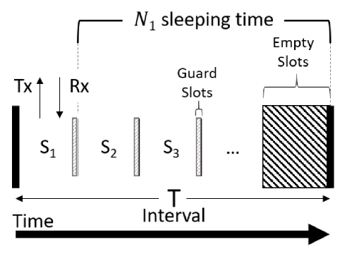
Figure 1: Simplistic TDMA MAC Protocol.

TDMA is a channel access method for shared medium networks, which allows several users to share the same frequency channel. Specifically, time is divided into intervals $T_{i}$ with length $T$, so-called super-frames. Each interval is split into smaller time slots $S_{j}$, with $\sum\limits_{j=1}^{N}S_{j}\leq T$, where $N$ is the number of sensor/actuator nodes which share the same channel. In each time slot, only one predefined sensor/actuator node $N_{j}$ can transmit ($T_{x}$) or receive ($R_{x}$) a burst of messages to and from a base station. Outside the timeslot $S_{j}$, $N_{j}$ sleeps or executes other tasks depending on the hardware infrastructure and the provided ability to duty cycle. To avoid time violations of time slot bounds due to $N_{j}$ possible clock drift, a guard slot forces the termination of communication before the end of each $S_{j}$. Figure 1 illustrates the communication scheme of a simplistic TDMA protocol.

Due to synchronous operation, a TDMA-based protocol (e.g. [34]) can guarantee tight bounds on delays which are critical for network control systems. On the other hand, synchronizing sensor/actuator nodes is considered as the main drawback of TDMA-based systems. However, state of the art solutions, i.e. GPS clock synchronization technologies [40], ensure typical accuracy better than 1 microsecond by consuming ultra low power.

III-B C-TDMA and TTC & PETC

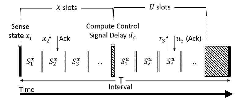
Figure 2: CTDMA protocol.

Control-TDMA (C-TDMA) is designed to enable TTC and PETC approaches (see Figure 2). In order to ensure the simultaneous state sampling, in the beginning of every interval $T_{i}$ at time $t_{i}$, every node $N_{j}$ has to retrieve a state measurement $x_{j}$ from the available sensors. Then, the channel bandwidth is divided into two sets of time slots which are separated by a time delay:

III-B1 Measurement Slots $\mathbf{S_{j}^{x}}$ (X-slots)

Every sensor/actuator node $N_{j}$ transmits $x_{j}$ within the time slot $S_{j}^{x}$ to the controller. Within each time slot only one successful message is required. Thus, the size selection of $S_{j}^{x}$ is application specific and depends on the size of $x_{j}$ (e.g. 2 Bytes per sensor) and the number of re-transmissions to achieve high reliability based on the selected hardware.

III-B2 Delay $\mathbf{d_{c}}$

After receiving the complete sampled state by receiving $x_{j},\forall j\in N$, a time delay is required to allow the computation of appropriate control signals $u_{j}$ for every sensor/actuator node $N_{j}$. The length of this delay depends on the controller infrastructure and the complexity of the control model.

III-B3 Actuation Slots $\mathbf{S_{j}^{u}}$ (U-slots)

The last set of time slots is related to the control message retrieval by the sensor/ actuator nodes $N_{j}$. In each time slot $S_{j}^{u}$, node $N_{j}$ transmits a request $r_{j}$ for a control signal $u_{j}$ to the controller. Then, the $u_{j}$ is piggybacked to the acknowledgement message. The benefit of the $r_{j}$ request is two-fold: (a) off-loads the controller side and (b) reduces $N_{j}$ listening time. Otherwise, the controller has to transmit or broadcast $u_{j}$ continuously by blocking other tasks, while $N_{j}$ has to be active in receive mode during the full length of the $S_{j}^{u}$ slot until a successful control message retrieval. Further, this approach causes more energy savings for nodes with communication modules that consume the same amount of energy for transmission and listening, i.e. [41]. The length of $S_{j}^{u}$ depends on the size of $u_{j}$ signals.

Based on the above, the minimum interval size $T_{min}$ can be defined by the length of X-slots, U-slots and delay $d_{c}$, and the number of the nodes. Further, the $T_{min}$ can be considered as the maximum time delay of the system.

TTC and PETC are centralized approaches and are executed in the controller. In both cases, the system requires the transmission of the current state to the controller at every $T_{i}$ during the X-slots. Then, in the TTC technique, the controller replies back in the U-slots of every interval $T_{i}$ with a new $u_{j}$ control signal. On the other hand, in PETC, the controller evaluates the event condition, as has been described in Equation (7), and transmits the new $u_{j}$ only if there is a violation. This behaviour allows PETC to save energy due to actuation reduction.

III-C SDC-TDMA and PSDETC

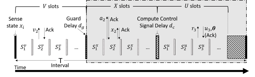
(a) SDC-TDMA Protocol for PSDETC approach.

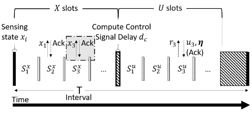
(b) ADC-TDMA Protocol for PADETC approach.

Figure 3: Communication schemes for decentralized ETC techniques.

PSDETC is a distributed technique and each sensor node is responsible for the state transmission decision in every $T_{i}$. The computation of control signals $u_{j}$ and $\theta_{j}$ parameters require the complete knowledge of the system’s state for the interval $T_{i}$ in which a threshold violation has happened. For example, consider a system with three nodes, $\{N_{1},N_{2},N_{3}\}$, in which only two of the nodes, i.e. $\{N_{2},N_{3}\}$, observe threshold violations. The controller requires the state from all the three nodes to compute the control signals. Using the same example, in a TDMA-based communication scheme in which each node is assigned to a pre-defined time slot $S_{j}$, node $N_{1}$ is precluded from transmitting its state by being unable to be informed about the threshold violations of $N_{2}$ and $N_{3}$. To overcome these limitations, SDC-TDMA introduces a new set of time slots $S_{j}^{v}$, the V-slots (see Figure 3(a)).

III-C1 Violations Slots $\mathbf{S_{j}^{v}}$ (V-slots)

In the beginning of every $T_{i}$, each node retrieves a measurement and evaluates Equation (9). Then, the result of each threshold $v_{j}$ is transmitted by the corresponding node $N_{j}$ to the controller at time slot $S_{j}^{v}$.

III-C2 Measurement Slots $\mathbf{S_{j}^{x}}$ (X-slots)

In the beginning of every $S_{j}^{x}$ in X-slots, each node $N_{j}$ asks the controller, by sending an $a_{j}$ request, whether a threshold violation was observed in the V-slots. If no threshold violation occurred, the sensor node sleeps immediately until the next interval $T_{i+1}$ (gray box in Figure 3(a)). Otherwise, each node transmits each state $x_{j}$ to controller, wait for the delay $d_{c}$ and actuation slots, U-slots, follow.

III-C3 Delay $\mathbf{d_{c}}$ & Actuation Slots $\mathbf{S_{j}^{u}}$ (U-slots)

Similar to the C-TDMA approach, after a delay $d_{c}$, each node requests the new control signal $u_{j}$ from the controller. The $u_{j}$ and the new threshold parameters $\theta_{j}$, which is being calculated based on Equation (10), are being piggybacked into the acknowledgement messages of U-slots.

Based on the above, SDC-TDMA sacrifices channel availability and increases the minimum interval length, $T_{min}$ and consequently the system’s maximum delay, by adapting V-slots into the TDMA scheme. However, in the case of threshold violation absence, the communication is being minimized significantly by avoiding the transmission of state $x_{j}$ and the entire execution of U-slots.

III-D ADC-TDMA and PADETC

Similar to PSDETC, the PADETC approach transfers the communication decision making from the controller down to the sensor/actuator nodes. Additionally, due to its asynchronous feature, this approach increases the communication savings by avoiding the state transmission $x_{j}$ from every node $N_{j}$ in every interval $T_{i}$. The only overhead in the communication is the $\eta_{j}$ update based on Equation (14) and transmission to $N_{j}$. The value of $\eta_{j}$ is being piggybacked with the control signal $u_{j}$ in the acknowledgement message.

Specifically, the architecture of ADC-TDMA is similar to C-TDMA and consists of sensing task, X-slots, $d_{c}$ delay, and U-slot (see Figure 3(b)). In a $S_{j}^{x}$ slot, the node $N_{j}$ evaluates the threshold of Equation (13). In the case of no threshold violation (i.e. gray box of Figure 3(b)), the node $N_{j}$ skips the communication and returns to sleep mode until $S_{j}^{u}$. Otherwise, $N_{j}$ transmits to the controller: $x_{j}$ in PADETCabs or the increment $m_{j}$ in PADETCrel (see Section II-D). Then, the controller computes the appropriate control signals and updates the local and global $\eta$ based on Equation (14) by using only the available $x_{j}$ states.

In the U-slots, every node has to send a $r_{j}$ request message to the controller, in order to be notified about a possible threshold violation from another node. Therefore, the violation of at least one threshold causes the update of $u_{j}$ and $\eta_{j}$ to be sent to every actuator node. The values of $u_{j}$ and $\eta_{j}$ are piggybacked to the acknowledgement message.

IV Evaluation Platform: WaterBox

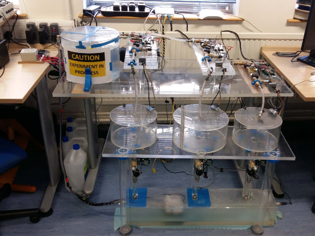
Figure 4: WaterBox Testbed.

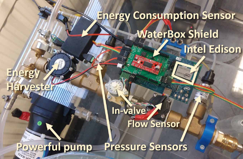
(a) WaterBox sensor/ actuator node.

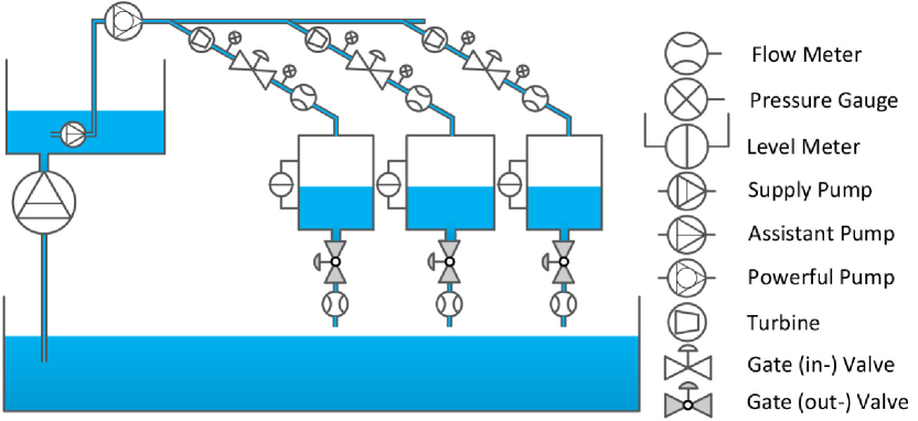
(b) The schematic structure of the WaterBox.

Figure 5: WaterBox evaluation platform.

Smart water networks have been used as a proof of concept for our proposed framework. The WaterBox platform (see Figure 4) is a scaled version of such water network [35] and developed to demonstrate real time monitoring and control by adapting innovative communication theories and control methodologies. WaterBox was used as evaluation platform for our proposed ETC techniques and communication schemes.

IV-A WaterBox infrastructure

A Water supply network structure consists of three individual layers: (a) storage and pumping, (b) water supply zones and District Meter Areas (DMAs), and (c) end users (water demand). While valves control flows and pressures at fixed points in the water network, pumps pressurise water to overcome gravity and frictional losses along supply zones, which are divided into smaller fixed network topologies (in average 1500 customer connections) with permanent boundaries, DMAs. The DMAs are continuously monitored with the aim to enable proactive leakage management, simplistic pressure management, and efficient network maintenance. WaterBox was designed to support this architecture as follows:

IV-A1 Water Storage and Pumping

The structure of the WaterBox is shown as Fig. 5(b). The WaterBox has a lower tank (i.e. ground, soil), an upper tank (i.e. reservoir, lake) and three small tanks (i.e. DMAs). The lower tank collects water from small tanks, and supplies water to the upper tank by an underwater bilge supply pump. This supply pump can supply enough water as the system requires. An assistant bilge pump and a new powerful pump are installed in series inside and after the upper tank respectively, and supply water to the small tanks. When the small tanks require more water supply, the assistant pump and powerful pump work together. When the small tanks require less water supply, only the assistant weak pump works. This behaviour emulates the day and night pumping operation of a water network in which the demand changes dramatically.

IV-A2 Water Supply & Sensor/Actuator Node

The water from the powerful pump flows into three small ’DMA’ tanks via a pipe network. For the inlet each tank, a sensor/actuator node (see Figure 5(a)), based on the Intel Edison development board [42], controls the water flow though a motorized gate valve, so-called in-valve, and monitors the water flow, pressure (before and after in-valve) and the in-tank water level. Further, a turbine (flow-based energy harvester) is installed before each in-valve to harvest energy. To capture the total energy consumption of each sensor/actuator node, a custom made sensor module was created.

Remark.

In the WaterBox infrastructure, the sensors and actuator of each inlet are connected to the same node. However, our proposed communication schemes can be applied to non-collocated infrastructures.

IV-A3 Water Demand Emulation

At the bottom of each small tank, there is an opening which enables the emulation of water consumption. A gate valve, so-called out-valve, is installed after each opening and can be controlled by a sensor/actuator node. The control of out-valves changes the outlet flow rate and facilitates the emulation of user’s random water consumptions (i.e. external disturbance).

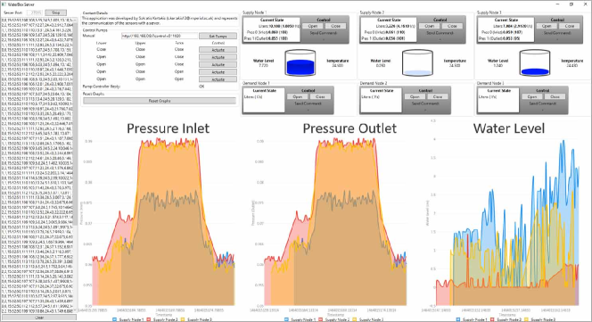
Figure 6: Local controller visualization application.

IV-A4 Base Station (Controller)

Every sensor node is connected to a local isolated WiFi network . A laptop is used as a controller or base station and hosts a visualization application (see Figure 6) which presents at real time the current state of the system, allows the manual control of actuators, logs the retrieved messages, and enables our proposed communication schemes and ETC scenarios per experiment. Additionally, due to lack of an indoor GPS time synchronization, a NTP server is running in the local controller and ensures less than millisecond time synchronization accuracy among the nodes.

IV-B System Identification & Modelling

We apply Grey-Box identification [43] to generate the system model and to find the uncertain parameters. A first principles model is obtained following [44]. We identify independently models under both mode 1: only the assistant pump works and mode 2: both pumps work. Using the Matlab cftool, we generate fitting curves for the gate valve coefficient of each in-valve, the turbine efficiency, and the pump efficiency. These curves are used to compute the first principles model. Since our aim is to stabilize the water level of each tank $j\in\{1,2,3\}$ at the desired height $h_{j}^{\prime}$, the model is linearised around this height. In this process, in order to simplify the simulation of the user water consumption, we keep the out-valves open, thus, constant out flow rates can be assumed.

V Hybrid Controller Design

To evaluate the proposed ETC-based communication schemes, the following control scenario was used: ”Control in-valves to stabilize the water level of the small ’DMA’ tanks to a certain level ensuring pressure and flow bounds. Enable mode 2 (weak and powerful pump) only if the system is away from the target levels. Switch to mode 1 (weak pump) only when the system is close to the reference state to guarantee efficient low pressure and flow operation.”

V-A Hybrid Controller Design

In the design of the controller, the following limitations need to be considered:

1. Saturation of the actuators: The maximum open level of one in-valve is $360^{\circ}$, while the minimum is $0^{\circ}$.

2. Actuator quantization: Due to the limitation of the valve’s control components, their open levels can only be changed in steps of $10^{\circ}$. Therefore, small disturbances may result in dramatic changes of actuations.

3. Over-pressure protection: Due to mechanical limitations of the pipe network, there is a maximum allowable pressure for the pipe network.

Since the height of the water levels have a direct effect on the Quality of Service (QoS), the closed-loop system requires a fast response; however, since the size of the small tanks are limited, the overshoot should simultaneously be constrained. Experiments show that, in mode 2, the pipe network may be over pressured, when the open level of the in-valves, defined by $\alpha_{j}^{in}$, cannot satisfy:

$$\sum_{j=1}^{3}\alpha_{j}^{in}\geq 180^{\circ}.$$ (18)

Overshoot and disturbances could make condition (18) be violated. While in mode 1, there is no such constrains, that is, even all three in-valves are totally closed, the pipe network will not be over pressured. Therefore, filling the small tanks in mode 2 and switching to mode 1 when (18) is violated is required. Also experimentally, we observe that, when the system is in mode 1, the pump may not provide enough water supply to the small tanks even at the maximum open level, i.e. $\alpha_{j}^{in}=360^{\circ},\leavevmode\nobreak\ \forall j\in\{1,2,3\}$. Therefore, switching back to mode 2 when the water in the tanks reaches some pre-defined low levels is necessary. To support this mode switching, we define $\underline{h}:=\begin{bmatrix}\underline{h}_{1}&\underline{h}_{2}&\underline{h}_{3}\\ \end{bmatrix}^{\mathrm{T}},\,\underline{h}_{j}<h^{\prime}_{j},\,j\in\{1,2,3\}$, as the lower water levels. If $\exists j\in\{1,2,3\}$ such that $h_{j}(t)\leq\underline{h}_{j}$, the system switches from mode 1 to mode 2. With carefully chosen $\underline{h}_{j}$ and properly designed controllers, this violation can only happen in mode 1. Further analysis shows that, (18) can only be violated when $h_{j}(t)>h_{j}^{\prime}$, which together with the fact that $\underline{h}_{j}<h^{\prime}_{j}$ precludes Zeno behaviour.

Let $\vartheta\in\{1,2\}$ represents the corresponding system mode. The linearised switched model and switched controller of WaterBox are described by:

$$\dot{\xi}(t)=A\xi(t)+B_{\vartheta}v(t),\,\vartheta=1,2,$$ (19)

$$v(t)=S(-K_{\vartheta}\xi(t)+\bar{\alpha}_{\vartheta}^{in}),\,\vartheta=1,2,$$ (20)

where $\xi(t)=\begin{bmatrix}\xi_{1}(t)&\xi_{2}(t)&\xi_{3}(t)\\ \end{bmatrix}^{\mathrm{T}}$, $\xi_{j}(t):=h_{j}(t)-h_{j}^{\prime},\,j=1,2,3$ are the system states, $h_{j}(t)\in\mathbb{R}$ are the water levels, and $h_{j}^{\prime}\in\mathbb{R}$ are the reference water levels; $v(t)=\begin{bmatrix}v_{1}(t)&v_{2}(t)&v_{3}(t)\\ \end{bmatrix}^{\mathrm{T}}$, $v_{j}(t):=\alpha_{j}^{in},\,j=1,2,3$ are the system control inputs, and $\bar{\alpha}_{\vartheta}^{in}$ are the equilibrium open levels of the in-valves per operation mode $\vartheta$; $S$ is a map $\mathbb{R}^{m}\rightarrow\mathbb{R}^{m}$ representing actuator saturation and quantization, that is $S(s_{j}):=\max\{\min\{10\lfloor 10^{-1}s_{j}\rfloor,360^{\circ}\},0^{\circ}\}$.

Then, the WaterBox hybrid controller state automaton is illustrated in Figure 7.

Figure 7: Hybrid controller state automaton.

From Grey-Box identification procedure, the system parameters are: $A$ is a zero $3\times 3$ matrix and

$$B_{1}=10^{-5}\times\scriptsize{\begin{bmatrix}0.1436&-0.0170&-0.0164\\ -0.0098&0.1060&-0.0100\\ -0.0139&-0.0139&0.1492\\ \end{bmatrix}},$$

$$\leavevmode\nobreak\ \leavevmode\nobreak\ B_{2}=10^{-5}\times\scriptsize{\begin{bmatrix}0.7666&-0.0493&-0.0457\\ -0.0274&0.5848&-0.0279\\ -0.0393&-0.0432&0.7865\\ \end{bmatrix}}.$$

The controllers designed are given by:

$$K_{1}=\scriptsize{\begin{bmatrix}99950&3029&872\\ -3014&99940&-1679\\ -922&1652&99982\\ \end{bmatrix}},K_{2}=\scriptsize{\begin{bmatrix}9998.5&167.1&41.0\\ -166.6&9997.9&-116.0\\ -43.0&115.3&9999.2\\ \end{bmatrix}}.$$

The designed controller is stable in both mode 1 and 2 because $-B_{1}K_{1}$ and $-B_{2}K_{2}$ are Hurwitz matrices. Further, due to the long dwell time of the system, the closed loop retains stability. Given $h_{j}^{\prime}=0.06$ and $\underline{h}_{j}=0.03$, $\forall j\in\{1,2,3\}$, $\bar{\alpha}_{1}^{in}$ and $\bar{\alpha}_{2}^{in}$ are computed:

$$\bar{\alpha}_{1}^{in}=\scriptsize{\begin{bmatrix}503.5950\\ 422.4378\\ 428.5839\\ \end{bmatrix}},\,\bar{\alpha}_{2}^{in}=\scriptsize{\begin{bmatrix}84.5099\\ 68.2069\\ 72.8442\\ \end{bmatrix}}.$$

VI Evaluation

This section summarizes the experimental results of more than 400 experiments conducted in WaterBox to evaluate our proposed communication schemes for the different ETC strategies. Each experiment executes the same control scenario (as described in Section V) and the total process lasts between 7 and 10 minutes, including the water state initialization, the execution of experiment, and data logging from sensor/ actuator nodes and local controller.

VI-A Evaluation Setup

Table I: Communication parameter evaluation setup.

	Parameter	Value	Description
Packet Size	$x_{j}$	36 Bytes	Node ID Timestamp (in msec) Inlet pressure Outlet pressure Flow rate Total water volume Distance from surface Energy consumption Energy harvesting
	$Ack$ — $r_{j}$, $a_{j}$	1 Byte	0 or 1 — Node ID
	$u_{j}$, $\eta_{j}$, $\theta_{j}$	2 Bytes	Control signal and DETC parameters
	$m_{j}$	4 Bytes	State delta
Time Duration	$S_{j}^{x}$	80 msec	X slot size
	$S_{j}^{u}$, $S_{j}^{v}$	50 msec	U and V slot size
	$d_{c}$	10 msec	Control decision delay
	$d_{g}$	5 msec	Threshold violation decision delay
	Guard slot	1 msec	Forced task termination time

The proposed communication protocols of Section III were deployed to the WaterBox sensor/actuator nodes by wrapping the functionality of the Intel Edison WiFi module. Table I presents the configuration of the communication parameters. Based on the predefined packet sizes of the specific hardware infrastructure, a set of experiments was conducted to determine reliable time slot and guard delay sizes.

Table II: Parameters of triggering strategies.

Method	$\mathbf{T}$ (sec)	Parameter	Value
TTC	0.5, 1, 2	-	-
PETC	0.5, 1, 2	$\sigma$	0.05, 0.1, 0.2
PSDETC	1, 2
PADETC (abs & rel)	0.5, 1, 2	$\mu$	0.75, 0.95
		$\varrho$	85, 120

Based on the Table I timing parameters and the Section III time slot analysis, the minimum interval size $T_{min}$ for C-TDMA and and ADC-TDMA has to be more than 321 msec while for SDC-TDMA more than 564 msec (because of the V-slots). Thus, we evaluate TTC, PETC, and PADETC (with absolute or reference value) with interval size $T=0.5,1,2$ and $T=1,2$ sec for PSDETC. The selected interval sizes and the rest parameters of the ETC strategies are listed in Table II. The $\sigma$ and $\rho$ ETC parameters are chosen by finding feasible solutions of the corresponding algorithms (8) and (17), while $\mu$ is tuned experimentally.

In the first set of experiments, we examine the impact of the ETC parameters ($\sigma$, $\mu$, and $\varrho$) to the performance of the system. A fixed interval size $T=1$ was used with all the different combinations of ETC parameter values of Table II. Another set of experiments was conducted to explore the effect of $T$ in the behaviour of the system. Keeping $\sigma=0.2$, $\mu=0.95$, and $\varrho=85$ constant, all the experiments were re-executed with $T=0.5$ and $T=2$ (Table II bold text). To ensure the validity of the evaluation results, each experiment was repeated 10 times for each different combination of ETC parameters and $T$. Mean values are used to illustrate the evaluation results. The data was captured from the nodes and controller for the period of time between the beginning of each experiment ($t_{0}=0$) until a fixed end time ($t_{end}=110s$), which guarantees the system turns to mode 1 and converges to steady state, denoted $T_{exp}$.

VI-B Experimental Results

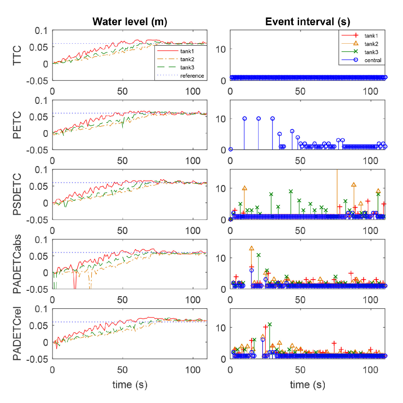
Figure 8: Experimental results. Note that, for SETC, the maximum event-interval of small tank 2 is 66 sec.

In this section we compare TTC, PETC, PSDET, PADETabs and PADETrel experimental results, in terms of:

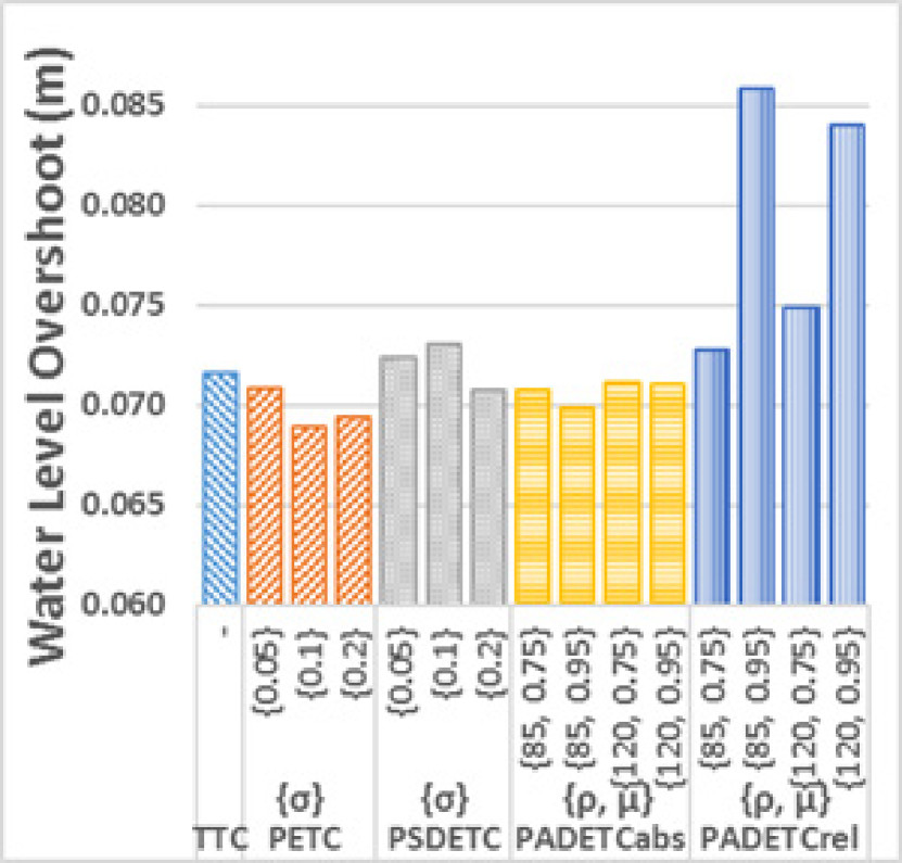
(a)

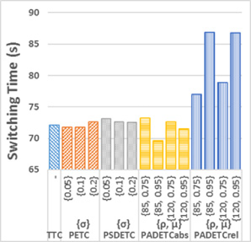
(b)

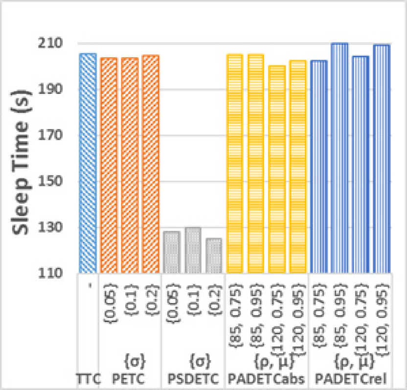
(c)

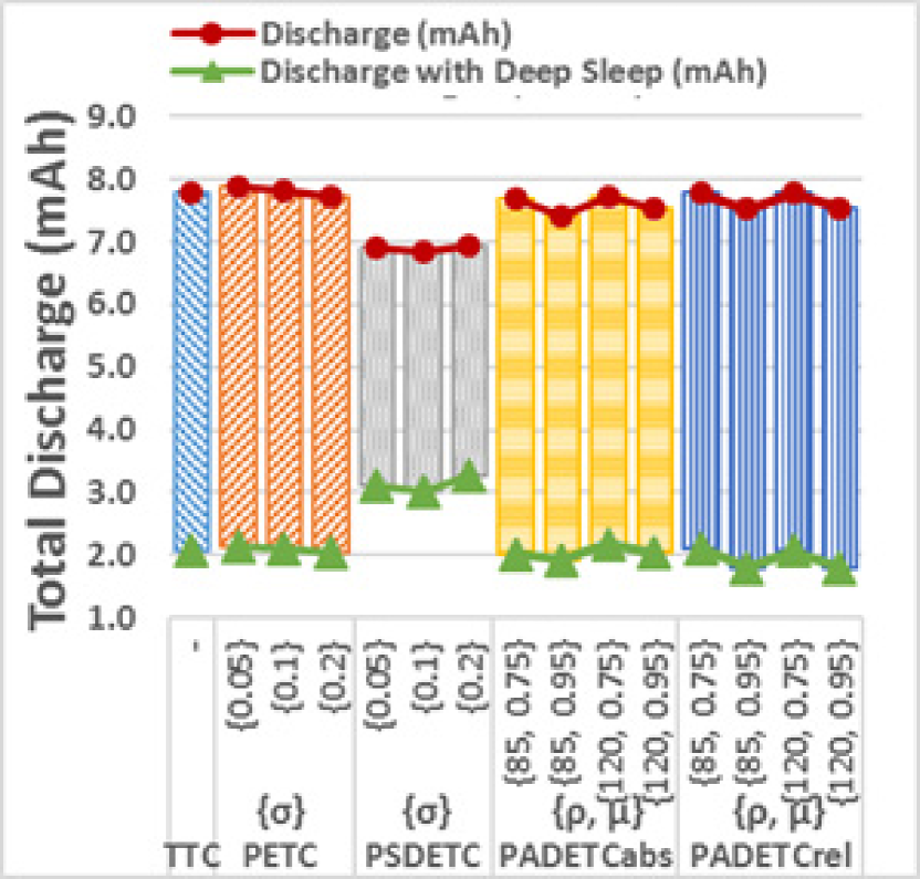
(d)

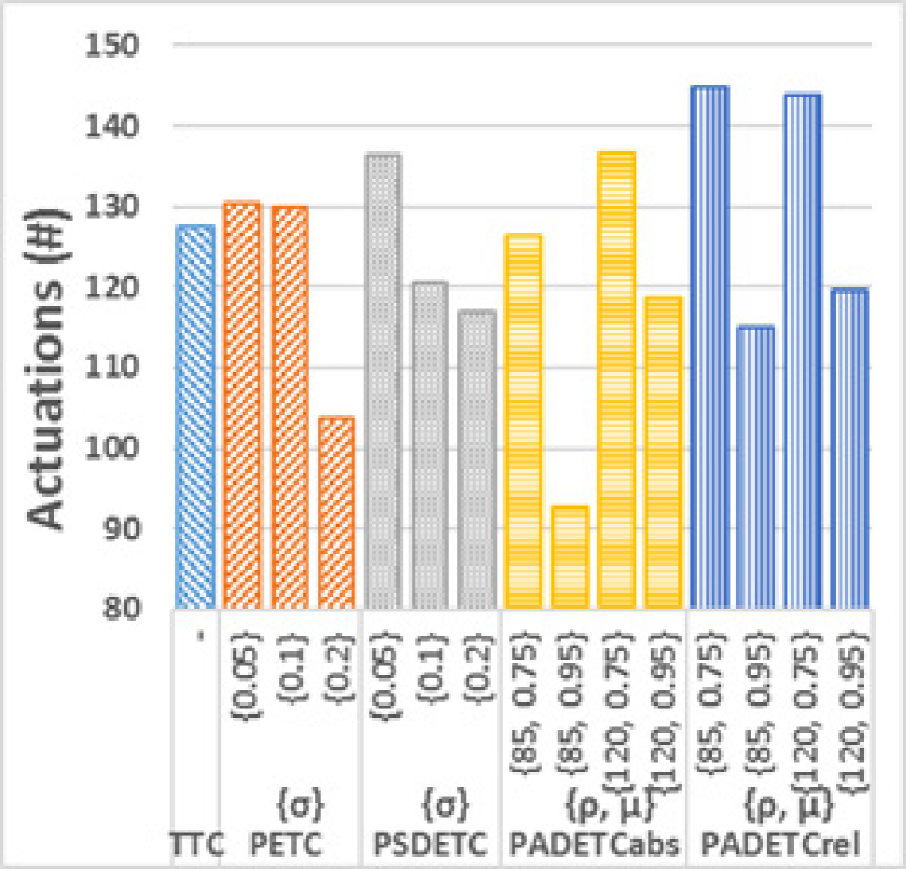
(e)

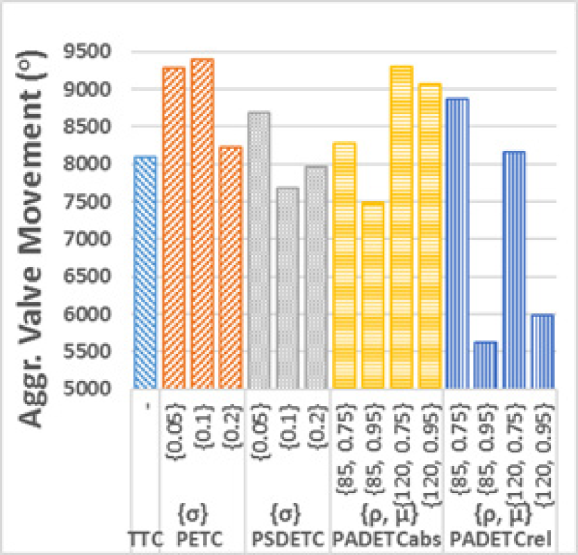
(f)

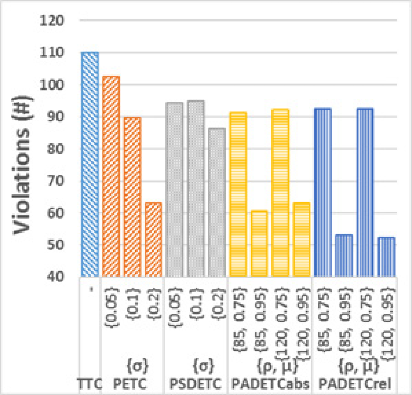
(g)

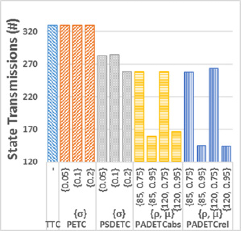
(h)

Figure 9: Impact of ETC parameters ($\sigma,\mu,\rho$) in: (a) water level overshoot, (b) switching time, (c) sleep time, (d) discharge, (e) actuations, (f) valve movement, (g) violation, and (h) state transmissions.

• Water Level Overshoot: the maximum water level during the experiment. This parameter indicates the system’s maximum state overshoot which is critical for water network asset safe operation.

• Switching Time ($t_{sm}$): the duration between experiment start time $t_{0}$ and first switch mode time $t_{sm}$, as described in condition (18). The time to mode switching is employed as an estimate of the system settling time (due to its ease of detection in our setup).

• Sleep Time: the total sleep time of all the nodes. This parameter evaluates the use of the bandwidth and CPU in the sensor/actuator node.

• Discharge (Energy Consumption): our custom made sensor module retrieves current measurements $c_{n}$ in mA at a fixed frequency of 10kHz. The energy consumption of a specific time period $\Delta t$ in seconds and with average current measurements over this period $\big{\langle}C\big{\rangle}_{\Delta t}$ can derived from $E(\Delta t)=\big{\langle}C\big{\rangle}_{\Delta t}\cdot\frac{\Delta t}{3600}$. We used a hardware average to ensure the continuity of the current measurements and validated our instrument against a calibrated reference [45]. The energy consumption includes the consumption because of the communication, sensing, actuation, and idle mode. We present two discharge values, i.e. the whole discharge and discharge without sleep time. Based on these parameters, the battery lifetime of different hardware infrastructures can be implied.

• Actuations: the number of valves’ changes, i.e. $\sum_{\forall{T_{i}}\in[t_{0},t_{end}]}\sum_{j=1}^{3}\alpha_{j}^{in}(T_{i})$. The amount of actuations indicates the lifetime of actuators which is vital for industrial deployments.

• Valve Movement: the sum of valves’ movement in degrees between two consecutive changes, i.e. $\sum_{\forall{T_{i}}\in[t_{0},t_{end}]}\sum_{j=1}^{3}|\alpha_{j}^{in}(T_{i})-\alpha_{j}^{in}(T_{i-1})|$. Combined with the number of actuations, the valve movement can be used to estimate physical system lifetime.

• Violations: the sum of event condition violations. For each violation the local controller transmits a control signal $u_{j}$ to each node i.e. three times. Therefore, the total transmitted control signal are equal to 3 times the violations. This metric indicates the communication requirements of actuators. Violations and actuations are different values because the local controller can produce the same consecutive control signal.

• State Transmissions: the sum of state $x_{j}$ transmissions to local controller. This metric indicates the communication requirements of sensors. Both violations and state transmissions represents the total communication requirements of the system.

Figure 8 shows an example of raw data as captured from the nodes and the controller. Next, we analyse the energy consumption trends compared to sleep time for different hardware infrastructures, the effect of ETC parameter setup and interval length $T$ to the performance of the system, and we aggregate the savings of ETC approaches against the vanilla scenario of TTC.

VI-B1 Energy Consumption and Sleep Time

The hardware infrastructure of a WaterBox node consumes more energy in sleep mode. During sleep mode, our process yields priority to the background tasks of the operating system which are more energy hungry. In order to generalize the results to different hardware infrastructures which support lower energy consumption during sleep mode (i.e. deep sleep), we provide the upper and a lower bounds of energy consumption. The upper bound presents the real experimental results based on our node while the lower bound represents an estimation of energy consumption of a node which supports deep sleep. The need of energy consumption range can be clearly seen in Figures 10(c) and 10(d). In spite of the sleep time increase in all cases, the upper bound of energy consumption increases proportionally (the opposite holds for the lower bound). Additionally, PSDETC is expected to consume more energy than the others because of the V-slots. However, Figures 9(c) and 9(d) illustrate the opposite trend for the upper bound (opposite for lower bound) due to the energy hungry sleep mode. Overall, PADETCabs and PADETCrel consume the least energy compared to the other approaches. In spite of the uses of the same communication scheme, PETC performs slightly better than TTC of actuation reduction (quantitative results will presented later on).

VI-B2 Effect of ETC Parameters

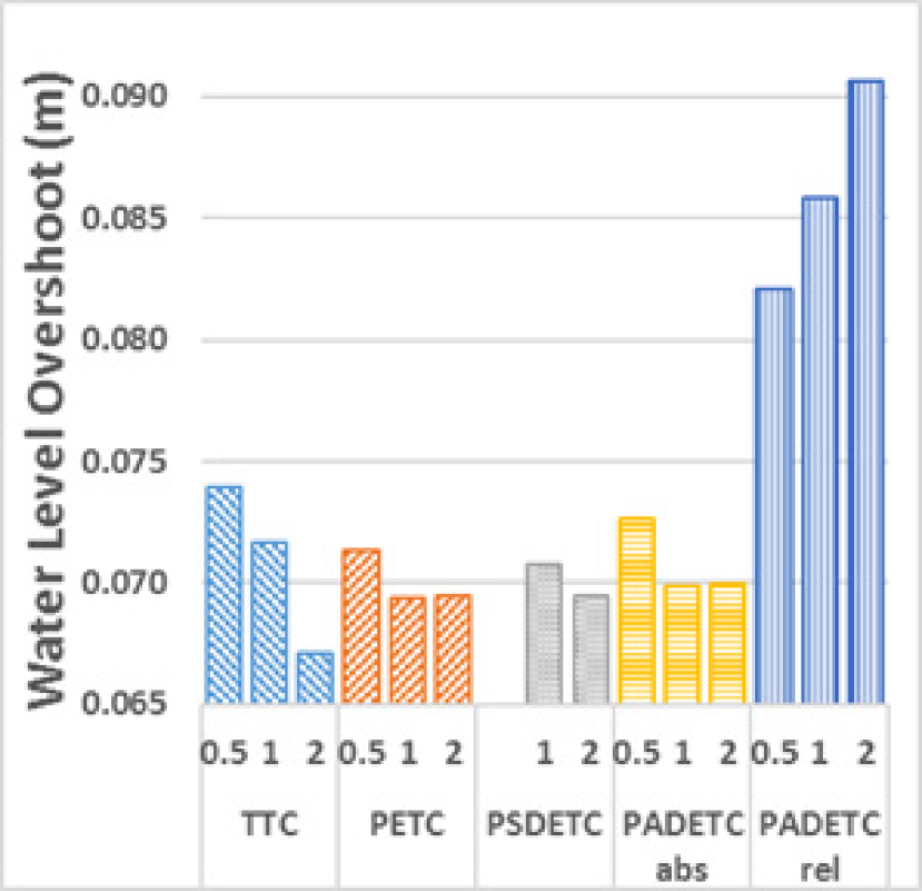
(a)

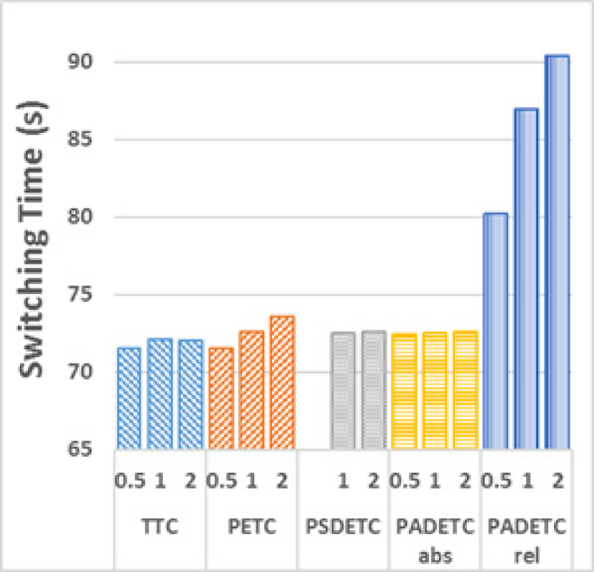
(b)

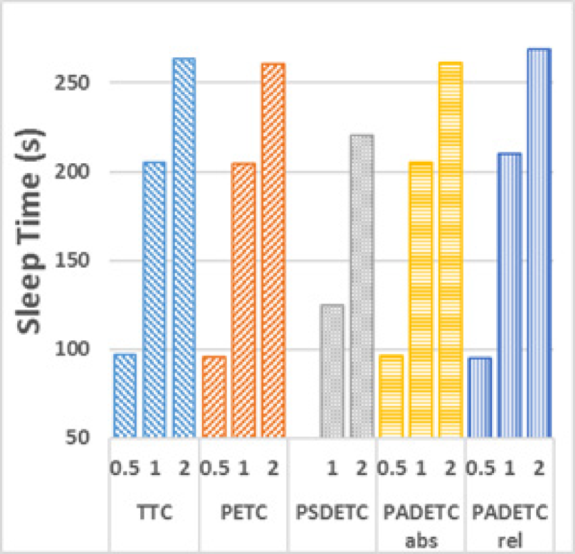
(c)

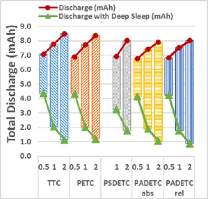
(d)

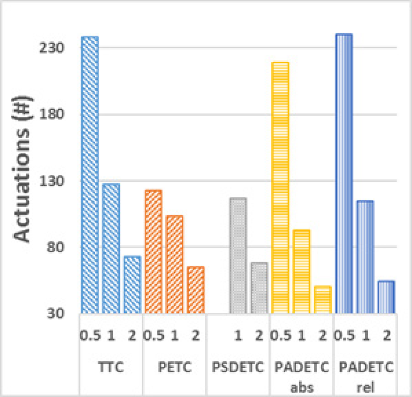
(e)

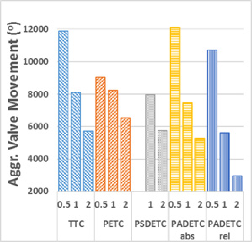
(f)

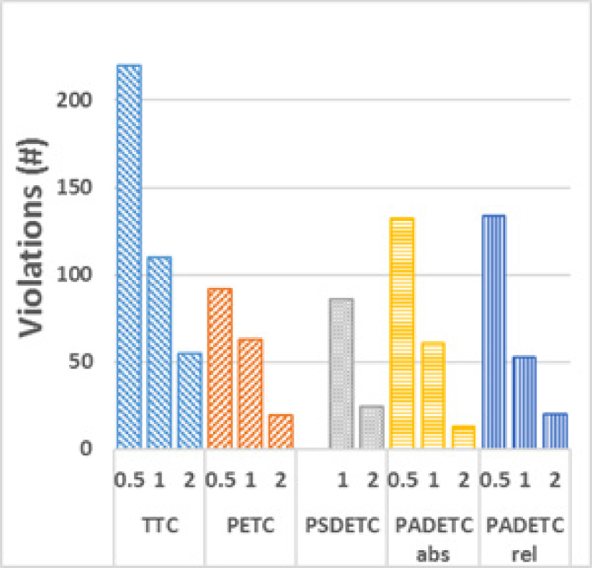
(g)

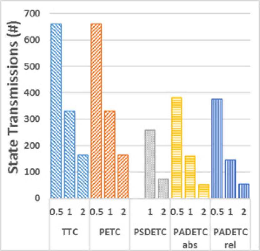
(h)

Figure 10: Impact of interval length $T$ in: (a) water level overshoot, (b) switching time, (c) sleep time, (d) discharge, (e) actuations, (f) valve movement, (g) violation, and (h) state transmissions.

Figure 9 presents the effect of different parameters, e.g. $\sigma$, $\rho$, $\mu$ with the same interval length $T=1$.The experiment results follow the trends shown in the theory. In PETC and PSDETC, a smaller $\mathbf{\sigma}$ forces the system to be more conservative and leads to more event condition violations (Figure 9(g)) and consequently to more actuation (Figure 9(e)) and energy consumption (Figure 9(d)). For the same reason, in the decentralized PSDETC, the state transmission reduces with bigger $\mathbf{\sigma}$ (Figure 9(h)).

In PADETC, a bigger $\mathbf{\varrho}$ has similar effect as a smaller $\sigma$ in PETC. This can be clearly seen in Figure 9(e) and 9(g), in which bigger $\mathbf{\varrho}$ causes more actuations and violations respectively. A bigger $\mathbf{\mu}$ can result in more frequent threshold updates, but maintains the threshold less conservative, and thus, the sampling errors can be enlarged. Additionally, Figure 9(g) shows that $\mu$ has greater impact on violations than $\sigma$ and $\varrho$ parameters.

VI-B3 Impact of Interval Length Selection

Figure 10 illustrates the impact of different interval lengths, in which the same pre-designed Lyapunov converge rate can be guaranteed, for the same set of rest of the parameters, e.g. $\sigma$, $\rho$, $\mu$. It can be clearly seen in Figure 10 that smaller interval $T$ results in better performance but worse energy consumptions. The water level overshoots are almost the same because of the actuator quantization. Larger sampling times always result in longer convergence time and longer sleeping times. Similarly, the upper bound discharge indicates this trend; longer sleep time leads to higher energy consumption due to the energy hungry operating system background tasks. Oppositely, the lower bound of discharge shows that hardware infrastructures with deep sleep consume significant lower energy for larger interval $T$ due to long sleeping time.

Table III: Savings compared to TTC (%) total experiment time, i.e. [0, $t_{end}$], with $\sigma=0.2,\rho=85$, and $\mu=0.95$

. Approach Water Level Overshoot Switching Time Discharge Discharge with Deep Sleep Actuations Aggr. Valve Movement Violations State Transmissions PETC 3.18 -0.69 0.97 1.1 18.6 -1.7 42.8 0 PSDETC 1.24 -0.55 11.03 -57.6 8.2 1.5 21.5 21.5 PADETC (abs) 2.44 3.47 4.74 6.9 27.2 7.5 44.8 51.6 PADETC (rel) -19.72 -20.53 3.28 13.2 9.7 30.5 51.8 56.0

Table IV: Savings compared to TTC (%) until mode switching time, i.e. [0, $t_{sm}$], with $\sigma=0.2,\rho=85$, and $\mu=0.95$

. Approach Water Level Overshoot Switching Time Discharge Discharge with Deep Sleep Actuations Aggr. Valve Movement Violations State Transmissions PETC 3.15 -0.69 1.34 2.4 30.3 17.3 55.2 -0.7 PSDETC 1.67 -0.55 10.97 -66.9 10.4 8.3 14.6 14.6 PADETC (abs) 3.02 3.47 9.22 11.9 34.7 24.1 57.0 63.9 PADETC (rel) -19.72 -20.53 -15.23 -4.5 14.4 22.6 49.1 54.5

VI-B4 Savings Compared to TTC

Table III and IV show the total savings of different ETC techniques against TTC for the time period $period_{1}=[0,t_{end}]$ (total experiment time) and $period_{2}=[0,t_{sm}]$ (time until switching mode) respectively. We provide this data separately due to the existence of the switched controller and the different behaviour of the two modes.

In $period_{1}$ PETC performs similarly to TTC with the difference of reduced actuations and violations by 18.6% and 42.8% respectively. In spite the saving, PETC causes more valve movements than TTC. The PSDETC is more conservative than the centralized PETC, with a result, the lower savings in terms of violations. However, PSDETC reduces the valve movements and the state transmissions due to the decentralized architecture. PADETCabs outperforms all the other approaches because of the asynchronous behaviour, reducing significantly the violations, state transmissions and actuations by achieving 44.8%, 51.6%, and 27.2% savings respectively. PADETCrel occurs similar actuation and communication saving with PADETCrel but with the trade-off of lower performance in terms of water level overshoots and switching time. As has been described in Section II, this happens because the PADETC with reference value updates introduces an extra error, known as maximum dynamic quantization error. However, this extra error allows this triggering mechanism to be more robust against noise than any of the other mechanisms with pre-designed maximum dynamic error.

In $period_{2}$, some ETC approaches deviate compared to the total savings. For example, in PETC approach, $period_{2}$ reveals higher actuation savings than $period_{1}$. The reason is that in mode 1, the weak pump is unable to supply the tanks with enough water and the system deviates from steady state continuously. Thus, event condition violations are being increased and often large valve movements are required. PSDETC and PADETCabs have a more stable behaviour than the other ETC approaches. Again PADETCabs outperforms the other ETC approaches achieving outstanding violation (57%) and actuation (35%) savings.

VII Conclusion

In this paper, we have proposed duty-cycling of the sensing and actuator listening activities and enabled decentralized ETC techniques introducing innovative communication schemes. Specifically, we designed and implemented three new MAC layers, which enable the application of four different periodic centralized and decentralized event triggered control approaches. By implementing our proposed communication schemes in the WaterBox testbed [35], we provided experimental results from more than 300 experiments.

Based on the experimental results, ETC approaches can introduce considerable benefits into industrial deployments. Due to the outstanding decrease of actuations either in number (up to 35%) or size (i.e. for valve movement up to 24%), the ETC techniques can increase the robustness, resilience, and lifetime of physical plants and actuators significantly. This increase can lead to significant maintenance cost reduction by postponing expensive replacements of plant assets.

WaterBox consists of energy hungry sensor/ actuator nodes to allow computational intensive algorithm deployments. An optimal hardware infrastructure will reduce the energy consumption even more than the evaluation results. Intuitively, the level of energy reduction will be closer to threshold violations (up to 57%) and state transmission (up to 64%) savings which indicate the actuator and sensors communication requirement respectively.

An additional benefit of applying periodic centralized or decentralized ETC approaches is the reduction of sensing rate. Continuous measurement retrieval from high energy demanding sensors (e.g. the water content sensor [46] which consumes 570 mJ per measurement) may lead to higher energy consumption than the communication process (e.g. low power wide area communication modules in [47] which consumes 1.5 to 42 J per 10 bytes). Further, based on our experimental results, higher sensing rates do not guarantee higher control performance. As future work, we will examine the aperiodic sensing scheduling over ETC techniques and the impact to the co-existing high sample rate algorithms for anomaly detection and validation. While in this paper we focus on smart water networks, the proposed framework can be applied to a variety of Cyber-Physical Systems such as Smart Grids, Smart Transportation Systems and Automated Agriculture.

References

- [1] SWIG, “Data standards and protocols for real-time communications in the water industry,” http://www.swig.org.uk/past-swig-events/2014-2/, 2015, online; accessed 22-June-2015.
- [2] P. Tabuada, “Event-triggered real-time scheduling of stabilizing control tasks,” IEEE Trans. Autom. Control, vol. 52, no. 9, pp. 1680–1685, 2007.
- [3] X. Wang and M. D. Lemmon, “Event-triggering in distributed networked control systems,” IEEE Trans. Autom. Control, vol. 56, no. 3, pp. 586–601, 2011.
- [4] W. Heemels, M. Donkers, and A. R. Teel, “Periodic event-triggered control for linear systems,” IEEE Trans. Autom. Control, vol. 58, no. 4, pp. 847–861, 2013.
- [5] M. Mazo Jr. and P. Tabuada, “Decentralized event-triggered control over wireless sensor/actuator networks,” IEEE Trans. Autom. Control, vol. 56, no. 10, pp. 2456–2461, 2011.
- [6] M. Mazo Jr. and M. Cao, “Asynchronous decentralized event-triggered control,” Automatica, vol. 50, no. 12, pp. 3197–3203, 2014.
- [7] B. A. Khashooei, D. J. Antunes, and W. Heemels, “An event-triggered policy for remote sensing and control with performance guarantees,” in Proc. IEEE CDC, 2015, pp. 4830–4835.
- [8] J. Sandee, P. Visser, and W. Heemels, “Analysis and experimental validation of processor load for event-driven controllers,” in Proc. IEEE CACSD, 2006, pp. 1879–1884.
- [9] W. Heemels, D. Borgers, V. Dolk, R. Geiselhart, and S. Heijmans, “Constructions of lyapunov functions for large-scale networked control systems with packet-based communication,” in Proc. ECC, 2016, pp. 936–938.
- [10] B. V. Eekelen, N. Rao, B. A. Khashooei, D. Antunes, and W. Heemels, “Experimental validation of an event-triggered policy for remote sensing and control with performance guarantees,” in Proc. EBCCSP, 2016.
- [11] D. Lehmann and J. Lunze, “Extension and experimental evaluation of an event-based state-feedback approach,” Control Engineering Practice, vol. 19, no. 2, pp. 101–112, 2011.
- [12] M. Sigurani, C. Stöcker, L. Grüne, and J. Lunze, “Experimental evaluation of two complementary decentralized event-based control methods,” Control Engineering Practice, vol. 35, pp. 22–34, 2015.
- [13] F. Altaf, J. Araújo, A. Hernandez, H. Sandberg, and K. H. Johansson, “Wireless event-triggered controller for a 3d tower crane lab process,” in Proc. IEEE MED, 2011, pp. 994–1001.
- [14] M. Lemmon, “Event-triggered feedback in control, estimation, and optimization,” in Networked Control Systems. Springer, 2010, pp. 293–358.
- [15] S. Trimpe and R. D’Andrea, “An experimental demonstration of a distributed and event-based state estimation algorithm,” IFAC, vol. 44, no. 1, pp. 8811–8818, 2011.
- [16] L. Orihuela, P. Millán, C. Vivas, and F. R. Rubio, “Suboptimal distributed control and estimation: application to a four coupled tanks system,” International Journal of Systems Science, vol. 47, no. 8, pp. 1755–1771, 2016.
- [17] T. Blevins, M. Nixon, and W. Wojsznis, “Event based control applied to wireless throttling valves,” in Proc. IEEE EBCCSP, 2015, pp. 1–6.
- [18] B. Boisseau, S. Durand, J. Martinez-Molina, T. Raharijaona, and N. Marchand, “Attitude control of a gyroscope actuator using event-based discrete-time approach,” in Proc. IEEE EBCCSP, 2015, pp. 1–6.
- [19] J. Araújo, M. Mazo Jr., A. Anta, P. Tabuada, and K. H. Johansson, “System architectures, protocols and algorithms for aperiodic wireless control systems,” IEEE Trans. Ind. Informat., vol. 10, no. 1, pp. 175–184, 2014.
- [20] M. Miskowicz and J. Lunze, “Event-based control: Introduction and survey,” in Event-Based Control and Signal Processing. CRC Press, 2015, pp. 3–20.
- [21] R. Blind and F. Allgöwer, “On time-triggered and event-based control of integrator systems over a shared communication system,” Mathematics of Control, Signals, and Systems, vol. 25, no. 4, pp. 517–557, 2013.
- [22] A. Cervin and T. Henningsson, “Scheduling of event-triggered controllers on a shared network,” in Proc. IEEE CDC, 2008, pp. 3601–3606.
- [23] C. Ramesh, H. Sandberg, and K. H. Johansson, “Stability analysis and design of a network of event-based systems,” arXiv preprint arXiv:1401.5004, 2014.
- [24] B. Demirel, V. Gupta, D. E. Quevedo, and M. Johansson, “On the trade-off between control performance and communication cost in event-triggered control,” arXiv preprint arXiv:1501.00892, 2015.
- [25] C. Ramesh, H. Sandberg, and K. H. Johansson, “Steady state performance analysis of multiple state-based schedulers with csma,” in Proc. IEEE CDC-ECC, 2011, pp. 4729–4734.
- [26] R. Blind and F. Allgöwer, “Analysis of networked event-based control with a shared communication medium: Part i–pure aloha,” Proc. IFAC, vol. 44, no. 1, pp. 10 092–10 097, 2011.
- [27] M. Vilgelm, M. H. Mamduhi, W. Kellerer, and S. Hirche, “Adaptive decentralized mac for event-triggered networked control systems,” in Proc. ACM HSCC, 2016, pp. 165–174.
- [28] R. Obermaisser and W. Lang, “Event-triggered versus time-triggered real-time systems: A comparative study,” Event-Based Control and Signal Processing, p. 59, 2015.
- [29] M. Mazo Jr. and A. Fu, “Decentralized event-triggered controller implementations,” Event-Based Control and Signal Processing, p. 121, 2015.
- [30] F. Calì, M. Conti, and E. Gregori, “Dynamic ieee 802.11: design, modeling and performance evaluation,” in International Conference on Research in Networking. Springer, 2000, pp. 786–798.
- [31] G. Miao, J. Zander, K. W. Sung, and S. B. Slimane, Fundamentals of Mobile Data Networks. Cambridge University Press, 2016.
- [32] N. Abramson, “The aloha system: another alternative for computer communications,” in Proc. ACM Joint Computer Conference, 1970, pp. 281–285.
- [33] IEEE, “IEEE 802.15.4 Standard: Wireless Medium Access Control (MAC) and Physical Layer (PHY) Specifications for Low-Rate Wireless Personal Area Networks (WPANs),” http://www.ieee802.org/15/pub/TG4.html, 2006, [Online; accessed 12-September-2016].
- [34] H. C. Foundation, “WirelessHART Data Sheet,” http://www.hartcomm2.org, 2007, [Online; accessed 12-September-2016].
- [35] S. Kartakis, E. Abraham, and J. A. McCann, “Waterbox: A testbed for monitoring and controlling smart water networks,” in Proc. ACM CysWater, 2015, p. 8.
- [36] A. Fu and M. Mazo Jr., “Periodic asynchronous event-triggered control,” in In 55th IEEE Conf. Decision and Control, 2016. To appear.
- [37] E. D. Sontag, “Input to state stability: Basic concepts and results,” in Nonlinear and optimal control theory. Springer, 2008, pp. 163–220.
- [38] S. P. Boyd, L. El Ghaoui, E. Feron, and V. Balakrishnan, Linear matrix inequalities in system and control theory. SIAM, 1994, vol. 15.
- [39] R. Goebel, R. G. Sanfelice, and A. R. Teel, Hybrid Dynamical Systems: modeling, stability, and robustness. Princeton University Press, 2012.
- [40] Spectracom, “GPS Clock Synchronization,” http://spectracom.com/resources/essential-education/gps-clock-synchronization, 2008, [Online; accessed 12-September-2016].
- [41] TI, “CC430F5137 Communication Module,” http://www.ti.com/product/CC430F5137, 2016, [Online; accessed 12-September-2016].
- [42] Intel, “Intel Edison board,” http://www.intel.com/content/www/us/en/do-it-yourself/edison.html, 2015, online; accessed 14-September-2016.
- [43] L. Ljung, System Identification: Theory for the User, ser. Prentice Hall information and system sciences series, 1999.
- [44] T. M. Walski, D. V. Chase, D. A. Savic, W. Grayman, S. Beckwith, and E. Koelle, “Advanced water distribution modeling and management,” 2003.
- [45] Keysight Technologies, “N6705B DC Power Analyzer,” http://www.keysight.com/en/pd-1842303-pn-N6705B/dc-power-analyzer-modular-600-w-4-slots?nid=-35714.937221.00&cc=GB&lc=eng, 2016, [Online; accessed 12-October-2016].
- [46] Delta-T Devices, “WET-2 Sensor,” http://www.delta-t.co.uk/product-display.asp?id=940, 2016, [Online; accessed 12-October-2016].
- [47] S. Kartakis, B. D. Choudhary, A. D. Gluhak, L. Lambrinos, and J. A. McCann, “Demystifying low-power wide-area communications for city iot applications,” in Proc. ACM WiNTECH ’16, 2016, pp. 2–8.