Extension of the Günter derivatives to Lipschitz domains and application to the boundary potentials of elastic waves

Abstract

The scalar Günter derivatives of a function defined on the boundary of a three-dimensional domain are expressed as components (or their opposites) of the tangential vector rotational of this function in the canonical orthonormal basis of the ambient space. This in particular implies that these derivatives define bounded operators from $H^{s}$ into $H^{s-1}$ for $0\leq s\leq 1$ on the boundary of a Lipschitz domain, and can easily be implemented in boundary element codes. Regularization techniques for the trace and the traction of elastic waves potentials, previously built for a domain of class $\mathcal{C}^{2}$, can thus be extended to the Lipschitz case. In particular, this yields an elementary way to establish the mapping properties of elastic wave potentials from those of the Helmholtz equation without resorting to the more advanced theory for elliptic systems. Some attention is finally paid to the two-dimensional case.

1 Introduction

All along this paper, $\Omega^{+}$ and $\Omega^{-}=\mathbb{R}^{3}\smallsetminus\overline{\Omega^{+}}$ respectively designate a bounded Lipschitz domain of $\mathbb{R}^{3}$, and its exterior. As a result, $\Omega^{+}$ and $\Omega^{-}$ share a common boundary denoted by $\partial\Omega$. It is well-known that $\partial\Omega$ is endowed with a Lebesgue surface measure $s$, and that it has an unit normal $\boldsymbol{n}$ (see figure 1), defined $s$-almost everywhere, pointing outward from $\Omega^{+}$ (cf., for example, [1, p. 96]). Vectors with three components $a_{j}$ $\left(j=1,2,3\right)$, either real or complex, are identified to column-vectors

$$\boldsymbol{a}=\left[\begin{array}[c]{c}a_{1}\\ a_{2}\\ a_{3}\end{array}\right].$$

The bilinear form underlying the scalar product of two such vectors $\boldsymbol{a}$ and $\boldsymbol{b}$ is given by

$$\boldsymbol{a\cdot b}=\boldsymbol{a}^{\top}\boldsymbol{b}=\boldsymbol{b}^{\top}\boldsymbol{a=}\sum_{j=1}^{3}a_{j}b_{j}$$

where $\boldsymbol{a}^{\top}$ is the transpose of $\boldsymbol{a}$.

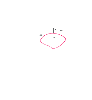
Figure 1: Schematic view of the geometry

Usual notation in the theory of Partial Differential Equations [2] will be used without further comment. We just mention that we make use of the following Fréchet spaces, defined for any integer $m\geq 0$ by

$$H_{\text{loc}}^{m}\left(\mathbb{R}^{3}\right)=\left\{v\in\mathcal{D}^{\prime}\left(\mathbb{R}^{3}\right);\;\varphi v\in H^{m}\left(\mathbb{R}^{3}\right),\;\forall\varphi\in\mathcal{D}\left(\mathbb{R}^{3}\right)\right\}$$

$$H_{\text{loc}}^{m}\left(\overline{\Omega^{-}}\right):=\left\{v\in\mathcal{D}^{\prime}\left(\Omega^{-}\right);\;\exists V\in H_{\text{loc}}^{m}\left(\mathbb{R}^{3}\right),\;v=V|_{\Omega^{-}}\right\},$$

and by

$$H_{\text{comp}}^{m}\left(\mathbb{R}^{3}\right)=\left\{v\in H^{m}\left(\mathbb{R}^{3}\right);\;\exists R>0,\;v|_{\left|x\right|\geq R}=0\right\}$$

$$H_{\text{comp}}^{m}\left(\overline{\Omega^{-}}\right)=\left\{v\in H^{m}\left(\Omega^{-}\right);\;\exists V\in H_{\text{comp}}^{m}\left(\mathbb{R}^{3}\right),\;v=V|_{\Omega^{-}}\right\}.$$

With similar definitions, it is trivially true that $H_{\text{loc}}^{m}\left(\overline{\Omega^{+}}\right)=H_{\text{comp}}^{m}\left(\overline{\Omega^{+}}\right)=H^{m}\left(\Omega^{+}\right)$. Below, we conveniently use the unified notation $H_{\text{loc}}^{m}\left(\overline{\Omega^{\pm}}\right)$ and $H_{\text{comp}}^{m}\left(\overline{\Omega^{\pm}}\right)$ to refer to both of these spaces. Instead of $H^{0}$, we use the more conventional notation $L^{2}$.

We denote by $u^{+}=\left(u|_{\Omega^{+}}\right)|_{\partial\Omega}$ (resp. $u^{-}=\left(u|_{\Omega^{-}}\right)|_{\partial\Omega}$) the trace of $u$ on $\partial\Omega$ from the values $u|_{\Omega^{+}}$ of $u$ in $\Omega^{+}$ (resp. $u|_{\Omega^{-}}$ in $\Omega^{-}$). For simplicity, we omit to explicitly mention the trace when the related function has zero jump across $\partial\Omega$. We also adopt a classical way to denote functional spaces of vector fields having their components in some scalar functional space. For example, $H^{s}\left(\partial\Omega;\mathbb{C}^{3}\right)$ stands for the space of vector fields $\boldsymbol{u}$ whose components $u_{j}$ $\left(j=1,2,3\right)$ are in $H^{s}\left(\partial\Omega\right)$.

For $1\leq i,j\leq 3$ and $u\in H_{\text{loc}}^{2}\left(\mathbb{R}^{3}\right)$, the Günter derivative

$$\mathcal{M}_{ij}^{\left(\boldsymbol{n}\right)}u=n_{j}\partial_{x_{i}}u-n_{i}\partial_{x_{j}}u$$ (1)

is well-defined as a function in $L^{2}\left(\partial\Omega\right)$ since the traces of $\partial_{x_{i}}u$ and $\partial_{x_{j}}u$ are in $H^{1/2}\left(\partial\Omega\right)$ and the components $n_{i}$ and $n_{j}$ of the normal $\boldsymbol{n}$ to $\partial\Omega$ are in $L^{\infty}\left(\partial\Omega\right)$. It is worth recalling that if $\Omega^{+}$ is a bit more regular, say a $\mathcal{C}^{1,1}$-domain for example (cf., [1, p. 90] for the definition of a $\mathcal{C}^{k}$-domain (resp. $\mathcal{C}^{k,\alpha}$-domain), also referred to as a domain of class $\mathcal{C}^{k}$ (resp. $\mathcal{C}^{k,\alpha}$)), $\mathcal{M}_{ij}^{\left(\boldsymbol{n}\right)}u$ is in $H^{1/2}\left(\partial\Omega\right)$. Seemingly, there is a loss of one-half order of regularity when considering a domain which is only Lipschitz. The purpose of this paper is precisely to show that this one-half order of regularity can be restored for functions in lower order Sobolev spaces.

Let us first recall some well-established properties of the Günter derivatives when $\Omega^{+}$ is at least a $\mathcal{C}^{1,1}$-domain. Let

$$\left\{\boldsymbol{e}_{j}=\left[\delta_{1j},\delta_{2j},\delta_{3j}\right]^{\top}\right\}_{j=1}^{3}\text{ (}\delta_{ij}=1\text{ if }i=j\text{ and }0\text{ otherwise)}$$

be the canonical basis of $\mathbb{R}^{3}$ so that $n_{j}=\boldsymbol{n}\cdot\boldsymbol{e}_{j}$ for $j=1,2,3$. Define for $1\leq i\neq j\leq 3$

$$\boldsymbol{\tau}_{ij}=n_{j}\boldsymbol{e}_{i}-n_{i}\boldsymbol{e}_{j}.$$ (2)

Clearly

$$\mathcal{M}_{ij}^{\left(\boldsymbol{n}\right)}u=\boldsymbol{\nabla}u\cdot\boldsymbol{\tau}_{ij}=\partial_{\boldsymbol{\tau}_{ij}}u$$

with

$$\boldsymbol{\tau}_{ij}\cdot\boldsymbol{n}=0.$$ (3)

As a result, $\mathcal{M}_{ij}^{\left(\boldsymbol{n}\right)}$ is a tangential derivative on $\partial\Omega$, meaning in particular, at least for $u\in\mathcal{C}^{1}\left(\mathbb{R}^{3}\right)$ and $\Omega^{+}$ a $\mathcal{C}^{1}$-domain, that $\mathcal{M}_{ij}^{\left(\boldsymbol{n}\right)}u$ can be calculated without resorting to interior values of $u$ in $\Omega^{+}$ or in $\Omega^{-}$.

These operators were introduced by Günter [3]. It was discovered later [4] that they can be used for bringing out important relations linking the boundary layer potentials of the Lamé system to those of the Laplace equation (see [4, p. 314] and [5, p. 48]). They were then employed to more conveniently express the traction of the double layer elastic potential (see [6] and [5, p. 49]). These approaches were recently extended to the elastic wave boundary layer potentials by Le Louër [7, 8]. All these results were derived under the assumption that $\Omega^{+}$ is a $\mathcal{C}^{2}$-domain (actually, $\mathcal{C}^{1,1}$- is enough). It is the aim of this paper, by defining the Günter derivatives for a Lipschitz domain, that is, a $\mathcal{C}^{0,1}$-domain, to similarly handle geometries more usual in the applications. More importantly, it is possible in this way to deal with boundary element approximations of the traction of single- and double-layer potentials of Lamé static elasticity and elastic wave systems almost as easily as for the Laplace or the Helmholtz equation.

Actually, in connection with elasticity potential layers, Günter derivatives are involved as entries $\mathcal{M}_{ij}^{\left(\boldsymbol{n}\right)}$ $\left(i,j=1,2,3\right)$ of the skew-symmetric matrix $\mathcal{M}^{\left(\boldsymbol{n}\right)}$ acting on vector-valued functions $\boldsymbol{u}$

$$\left(\mathcal{M}^{\left(\boldsymbol{n}\right)}\boldsymbol{u}\right)_{i}=\sum_{j=1}^{3}\mathcal{M}_{ij}^{\left(\boldsymbol{n}\right)}u_{j}\quad\left(i=1,2,3\right),$$

$\left(\mathcal{M}^{\left(\boldsymbol{n}\right)}\boldsymbol{u}\right)_{i}$ and $u_{j}$ $\left(j=1,2,3\right)$ being the respective components of $\mathcal{M}^{\left(\boldsymbol{n}\right)}\boldsymbol{u}$ and $\boldsymbol{u}$. In [5], this matrix is called the Günter derivatives in matrix form. We find it more convenient to refer to $\mathcal{M}^{\left(\boldsymbol{n}\right)}\boldsymbol{u}$ as the Günter derivative matrix.

The Günter derivative matrix actually give rise to a multi-faceted operator, with various expressions, which led to real progresses in the context of Lamé static elasticity boundary layer potentials [4, 5, 7, 6] or in the design of preconditioning techniques for the boundary integral formulations in the scattering of elastic waves [9]. Other ways to write $\mathcal{M}^{\left(\boldsymbol{n}\right)}$ do not seem to have been connected with the Günter derivatives [10, 11]. However, all these expressions require either interior values, as for example for above direct definition (1) of $\mathcal{M}_{ij}^{\left(\boldsymbol{n}\right)}$, or curvature terms of $\partial\Omega$ as recalled below, making problematic their effective implementation in boundary element codes or in a preconditioning technique. It is among the objectives of this paper to address this issue.

The outline of the paper is as follows. In section 2, we first show that $\mathcal{M}_{ij}^{\left(\boldsymbol{n}\right)}u$ corresponds to a component (or its opposite) of the tangential vector rotational $\boldsymbol{\nabla}_{\partial\Omega}u\times\boldsymbol{n}$ of $u$ in an orthonormal basis of the ambient space. This feature, in addition to some duality properties, enable us to define this derivative as a bounded operator from $H^{s}\left(\partial\Omega\right)$ into $H^{s-1}\left(\partial\Omega\right)$ for $0\leq s\leq 1$. This is actually equivalent to arguing that $u\rightarrow\boldsymbol{\nabla}_{\partial\Omega}u\times\boldsymbol{n}$ is a bounded operator from $H^{s}\left(\partial\Omega\right)$ into $H^{s-1}\left(\partial\Omega;\mathbb{C}^{3}\right)$ for $0\leq s\leq 1$, a result which was established for $s=1/2$ in [12] from a different technique. It then follows that its transpose, yielding the surface rotational $\boldsymbol{\nabla}_{\partial\Omega}\cdot\boldsymbol{u}\times\boldsymbol{n}$ of a vector field $\boldsymbol{u}$ [13, p. 73], defines also a bounded operator from $H^{s}\left(\partial\Omega;\mathbb{C}^{3}\right)$ into $H^{s-1}\left(\partial\Omega\right)$ for $0\leq s\leq 1$. It is worth noting that in [13, p. 73] the surface rotational was considered for tangential vector fields only. However, the cross-product involved in the expression of this operator makes it possible to extend this definition to a general vector field. We show then that Günter derivatives $\mathcal{M}_{ij}^{\left(\boldsymbol{n}\right)}$ can be expressed as differential forms to retrieve an integration by parts formula relatively to these operators on a patch of $\partial\Omega$. Even if this formula was already established by direct calculation in [3], we think that the formalism of differential forms is more appropriate for understanding the basic principle underlying its derivation. It is used here to get explicit expressions for the Günter derivatives of a piecewise smooth function defined on a the boundary of a curved polyhedron. This way to write these derivatives is fundamental in the effective implementations of boundary element codes. In section 3, we begin with some recalls on other previous expressions for Günter derivative matrix $\mathcal{M}^{\left(\boldsymbol{n}\right)}$. With the help of a vectorial Green formula, partly introduced in [14] and in a more complete form in [10, 11], we derive a useful volume variational expression for $\mathcal{M}^{\left(\boldsymbol{n}\right)}$. As an application in section 4, we extend the regularization techniques (the way for expressing non-integrable kernels involved in boundary layer potentials in terms of integrals converging in the usual meaning) devised by Le Louër [7, 8] for the elastic wave layer potentials to Lipschitz domains. It is worth recalling that due to its importance in practical implementations of numerical solvers for elastic wave scattering problems, several other regularizations techniques, much more involved in our opinion, have been already proposed (cf., for example, [15, 16, 17, 18, 19, 20] to cite a few). Finally, in Section 5, making use of the connection between two- and three-dimensional Green kernels for the Helmholtz equation, we transpose the regularization techniques in the spatial scale to planar elastic waves.

2 Extension of the Günter derivatives to a Lipschitz domain

We first establish some mapping properties of the Günter derivatives in the framework of a Lipschitz domain. We next show that they can be written as differential 2-forms, up to a Hodge star identification. This will allow us to retrieve an integration by parts formula on the patches of $\partial\Omega$. That yields an expression of these derivatives well suited for boundary element codes.

2.1 Mapping properties of the Günter derivatives for Lipschitz domains

Property (3) ensures that $\mathcal{M}_{ij}^{\left(\boldsymbol{n}\right)}$ is a first-order differential operator tangential to $\partial\Omega$ in the sense of [1, p. 147]. This immediately leads to the following first mapping property whose proof is given in Lemma 4.23 of this reference.

Proposition 1.

There exists a constant $C$ independent of $u\in H^{1}\left(\partial\Omega\right)$ such that

$$\left\|\mathcal{M}_{ij}^{\left(\boldsymbol{n}\right)}u\right\|_{L^{2}\left(\partial\Omega\right)}\leq C\left\|u\right\|_{H^{1}\left(\partial\Omega\right)}.$$ (4)

To go further, we make the following observation which, surprisingly enough, does not seem to have been done before.  It consists in noting that vector $\boldsymbol{\tau}_{ij}$, defined in (2), can be written under the following form using the elementary double product formula

$$\boldsymbol{\tau}_{ij}=\left(\boldsymbol{n}\cdot\boldsymbol{e}_{j}\right)\boldsymbol{e}_{i}-\left(\boldsymbol{n}\cdot\boldsymbol{e}_{i}\right)\boldsymbol{e}_{j}=\boldsymbol{n}\times\left(\boldsymbol{e}_{i}\times\boldsymbol{e}_{j}\right)\;\left(1\leq i,j\leq 3\right).$$

In this way, using the properties of the mixed product, we can also put Günter derivative $\mathcal{M}_{ij}^{\left(\boldsymbol{n}\right)}u$ in the following form

$$\mathcal{M}_{ij}^{\left(\boldsymbol{n}\right)}u=\boldsymbol{\nabla}u\cdot\boldsymbol{n}\times\left(\boldsymbol{e}_{i}\times\boldsymbol{e}_{j}\right)=\boldsymbol{\nabla}u\times\boldsymbol{n}\cdot\boldsymbol{e}_{i}\times\boldsymbol{e}_{j}.$$ (5)

Indeed, formula (5) expresses $\mathcal{M}_{ij}^{\left(\boldsymbol{n}\right)}u$ as a component (or its opposite) of the tangential vector rotational of $u$ in the canonical basis of $\mathbb{R}^{3}$

$$\mathcal{M}_{ij}^{\left(\boldsymbol{n}\right)}u=\boldsymbol{\nabla}_{\partial\Omega}u\times\boldsymbol{n}\cdot\boldsymbol{e}_{i}\times\boldsymbol{e}_{j}.$$

(See [13, p. 69] for the definition and properties of the tangential gradient $\boldsymbol{\nabla}_{\partial\Omega}u$ and the tangential vector rotational of a function when, for example, $\Omega^{+}$ is a $\mathcal{C}^{2}$-domain.)

We have next the following lemma which is established in a less straightforward way in [3] for a $\mathcal{C}^{1,\alpha}$-domain $\left(0<\alpha\leq 1\right)$.

Lemma 1.

For $u$ and $v$ in $\mathcal{C}_{\text{comp}}^{1}\left(\mathbb{R}^{3}\right)$, the following integration by parts formula

$$\int_{\partial\Omega}v\mathcal{M}_{ij}^{\left(\boldsymbol{n}\right)}u\ ds=\int_{\partial\Omega}u\mathcal{M}_{ji}^{\left(\boldsymbol{n}\right)}v\ ds$$ (6)

holds true.

Proof.

The proof directly follows from the following simple observation

$$\boldsymbol{\nabla}\times\left(uv\boldsymbol{e}_{i}\times\boldsymbol{e}_{j}\right)=v\boldsymbol{\nabla}\times\left(u\boldsymbol{e}_{i}\times\boldsymbol{e}_{j}\right)-u\boldsymbol{\nabla}\times\left(v\boldsymbol{e}_{j}\times\boldsymbol{e}_{i}\right)$$

and Green’s formula in Lipschitz domains [1, Th. 3.34]

$$\int_{\Omega^{\pm}}\underset{=0}{\underbrace{\boldsymbol{\nabla}\cdot\boldsymbol{\nabla}\times\left(uv\boldsymbol{e}_{i}\times\boldsymbol{e}_{j}\right)}}\ dx =\pm\int_{\partial\Omega}\left(\boldsymbol{\nabla}\times\left(uv\boldsymbol{e}_{i}\times\boldsymbol{e}_{j}\right)\right)\cdot\boldsymbol{n}ds$$

$$=\mp\left(\int_{\partial\Omega}v\mathcal{M}_{ij}^{\left(\boldsymbol{n}\right)}u\ ds-\int_{\partial\Omega}u\mathcal{M}_{ji}^{\left(\boldsymbol{n}\right)}v\ ds\right).$$

∎

We then come to the following theorem embodying optimal mapping properties of the Günter derivatives.

Theorem 1.

Under the above assumption that $\Omega^{+}$ is a bounded Lipschitz domain, Günter derivative $\mathcal{M}_{ij}^{\left(\boldsymbol{n}\right)}$ can be extended in a bounded linear operator from $H^{s}\left(\partial\Omega\right)$ into $H^{s-1}\left(\partial\Omega\right)$ for $0\leq s\leq 1.$

Proof.

It is a straightforward consequence of estimate (4) and symmetry property (6) by duality and interpolation techniques. ∎

Corollary 1.

Under the general assumptions of the above theorem, the tangential vector rotational defines a bounded linear operator $u\rightarrow\boldsymbol{\nabla}_{\partial\Omega}u\times\boldsymbol{n}$ from $H^{s}\left(\partial\Omega\right)$ into $H^{s-1}\left(\partial\Omega;\mathbb{C}^{3}\right)$ for $0\leq s\leq 1$. Consequently, the surface rotational gives rise to a bounded operator $\boldsymbol{u}\in H^{s}\left(\partial\Omega;\mathbb{C}^{3}\right)\rightarrow\boldsymbol{\nabla}_{\partial\Omega}\cdot\boldsymbol{u}\times\boldsymbol{n}\in$ $H^{s-1}\left(\partial\Omega\right)$ for $0\leq s\leq 1$.

Proof.

Immediate since the components of $\boldsymbol{\nabla}_{\partial\Omega}u\times\boldsymbol{n}$ are nothing else but Günter derivatives and the surface rotational is the transpose of the tangential vector rotational. ∎

Remark 1.

When $u$ and $v$ are the respective traces of functions in $H^{1}\left(\mathbb{R}^{3}\right)$, it is established in [12, p. 855] that $\boldsymbol{\nabla}u\times\boldsymbol{n}$ is well-defined in $H_{\|}^{-1/2}\left(\partial\Omega;\mathbb{C}^{3}\right)$, the dual space of

$$H_{\|}^{1/2}\left(\partial\Omega;\mathbb{C}^{3}\right)=\left\{\boldsymbol{v}\in L^{2}\left(\partial\Omega;\mathbb{C}^{3}\right);\;\boldsymbol{v}=\boldsymbol{n}\times(\boldsymbol{w}\times\boldsymbol{n}),\;\boldsymbol{w}\in H^{1}\left(\Omega^{\pm};\mathbb{C}^{3}\right)\right\}$$

equipped with the graph norm and that $\boldsymbol{\nabla}u\times\boldsymbol{n}$ depends on the trace $u|_{\partial\Omega}$ of $u$ on $\partial\Omega$ [12, p. 855] only. It is also proved in this paper [12, formulae (15) p. 850 and Lemma 2.3 p. 851] that $H_{\|}^{-1/2}\left(\partial\Omega;\mathbb{C}^{3}\right)$ can be identified to a closed subspace of $H^{-1/2}\left(\partial\Omega;\mathbb{C}^{3}\right)$. This is the particular case corresponding to $s=1/2$ which has been previously mentioned.

The following symmetry result is known for a long time in the case of smoother domains and more regular functions [4, p. 284] and is an immediate consequence of the definition of the Günter derivative matrix and the symmetry and mapping properties of $\mathcal{M}_{ij}^{\left(\boldsymbol{n}\right)}$.

Corollary 2.

Günter derivative matrix $\mathcal{M}^{\left(\boldsymbol{n}\right)}$ defines a bounded linear operator from $H^{s}\left(\partial\Omega;\mathbb{C}^{3}\right)$ into $H^{s-1}\left(\partial\Omega;\mathbb{C}^{3}\right)$ for $0\leq s\leq 1$ with the following symmetry property

$$\left\langle\boldsymbol{v},\mathcal{M}^{\left(\boldsymbol{n}\right)}\boldsymbol{u}\right\rangle_{1-s,\partial\Omega}=\left\langle\boldsymbol{u},\mathcal{M}^{\left(\boldsymbol{n}\right)}\boldsymbol{v}\right\rangle_{s,\partial\Omega},\;\boldsymbol{u}\in H^{s}\left(\partial\Omega;\mathbb{C}^{3}\right),\boldsymbol{v}\in H^{1-s}\left(\partial\Omega;\mathbb{C}^{3}\right).$$ (7)

For simplicity, we keep the same notation for the bilinear form underlying the duality product between $H^{s}\left(\partial\Omega;\mathbb{C}^{3}\right)$ and $H^{-s}\left(\partial\Omega;\mathbb{C}^{3}\right)$ and that $\left\langle\mathcal{\cdot},\cdot\right\rangle_{s,\partial\Omega}$ between $H^{s}\left(\partial\Omega\right)$ and $H^{-s}\left(\partial\Omega\right)$

$$\left\langle\boldsymbol{v},\boldsymbol{\ell}\right\rangle_{s,\partial\Omega}=\sum_{i=1}^{3}\left\langle v_{i},\ell_{i}\right\rangle_{s,\partial\Omega},\;\boldsymbol{\ell}\in H^{-s}\left(\partial\Omega;\mathbb{C}^{3}\right),\boldsymbol{v}\in H^{s}\left(\partial\Omega;\mathbb{C}^{3}\right).$$

Remark 2.

The duality $H^{s}\left(\partial\Omega\right)$, $H^{-s}\left(\partial\Omega\right)$ is usually denoted by $\left\langle\ell,v\right\rangle_{s,\partial\Omega}$ for $\ell\in H^{-s}\left(\partial\Omega\right)$ and $v\in H^{s}\left(\partial\Omega\right)$. The transposition used here is convenient for the notation of the single-layer potential of elastic waves given below.

2.2 Explicit expression for the Günter derivatives

Up to now, we have defined the Günter derivatives just in the distributional sense: $\mathcal{M}_{ij}^{\left(\boldsymbol{n}\right)}u\in$ $H^{s-1}\left(\partial\Omega\right)$ for $u\in H^{s}\left(\partial\Omega\right)$, $0\leq s\leq 1$. In concrete applications, $\partial\Omega$ must be considered as the boundary of a curved polyhedron. This is the case of course when $\partial\Omega$ presents curved faces and edges, and vertices, but also once the geometry has been effectively approximated (cf., for example, [21, p. 15]). This means that $\partial\Omega$ can be covered by a non-overlapping decomposition $\mathcal{T}$

$$\partial\Omega=\cup_{\omega\in\mathcal{T}}\overline{\omega}$$

where $\mathcal{T}$  is a finite family of open domains $\omega$ of $\partial\Omega$ such that for all $\omega,\upsilon\in\mathcal{T}$, $\omega\cap\upsilon=\emptyset$ when $\omega\neq\upsilon$. Each $\omega$ is assumed to be a  “surface polygonal domain” in the meaning that $\overline{\omega}\subset U_{\omega}$ ($U_{\omega}$ being an open $\mathcal{C}^{\infty}$-parametrized surface of $\mathbb{R}^{3}$), that its boundary $\partial\omega$ is a piecewise smooth curve, and that $\omega$ is a Liptchitz domain of $U_{\omega}$. Lipschitz domains of smooth manifolds are defined similarly to Lipchitz domains of $\mathbb{R}^{N}$ replacing “rigid motions” in [1, Definition 3.28] by local $\mathcal{C}^{\infty}$-diffeomorphisms onto domains of $\mathbb{R}^{2}$. Recall that $\Omega^{+}$ is globally a Lipschitz domain, hence preventing $\partial\Omega$ to present cusp points. Simple and widespread examples of such boundaries are given by triangular meshes of surfaces of $\mathbb{R}^{3}$. Figure 2 depicts a surface triangular mesh of a $C^{1,1}$-domain. The geometry and the mesh have been designed using the free software Gmsh [22]. For the exact surface, $\omega$ and $U_{\omega}$ are obtained by local coordinate systems (local charts) (see, for example, [23]). For the approximate surface, $\omega$ is a triangle of $\mathbb{R}^{3}$ and $U_{\omega}$ is the plane supporting this triangle.

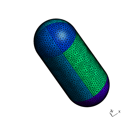
Figure 2: Polyhedral domain obtained from the surface mesh of $C^{1,1}$-domain.

Boundary element spaces are generally subspaces of the following one

$$\mathcal{P}_{m,\mathcal{T}}\left(\partial\Omega\right)=\left\{u\in L^{\infty}\left(\partial\Omega\right);\;u|_{\omega}\circ\Phi_{\omega}\in\mathbb{P}_{m},\;\forall\omega\in\mathcal{T}\right\}$$

where $\Phi_{\omega}:D_{\omega}\subset\mathbb{R}^{2}\rightarrow U_{\omega}$ is a local coordinate system on $U_{\omega}$ (cf., for example, [23, p. 111]). Such kinds of spaces are contained in $H^{s}\left(\partial\Omega\right)$ for $1/2\leq s\leq 1$ if and only if they are contained in

$$\mathcal{C}_{\mathcal{T}}\left(\partial\Omega\right)=\left\{u\in\mathcal{C}^{0}\left(\mathcal{\partial}\Omega\right);\;u|_{\omega}\in\mathcal{C}^{\infty}\left(\overline{\omega}\right),\;\forall\omega\in\mathcal{T}\right\}$$

(see, for example, [24] when $\partial\Omega=\mathbb{R}^{2}$).

For $u\in\mathcal{C}_{\mathcal{T}}\left(\partial\Omega\right)$, we can define $\mathcal{M}_{ij,\mathcal{T}}^{\left(\boldsymbol{n}\right)}u$ almost everywhere on $\partial\Omega$ by

$$\left(\mathcal{M}_{ij,\mathcal{T}}^{\left(\boldsymbol{n}\right)}u\right)|_{\omega}=\boldsymbol{\nabla}_{\omega}u|_{\omega}\times\boldsymbol{n}\cdot\boldsymbol{e}_{i}\times\boldsymbol{e}_{j},\;\forall\omega\in\mathcal{T}$$

where $\boldsymbol{\nabla}_{\omega}$ is the tangential gradient on $\omega$ and $\boldsymbol{n}$ is the unit normal on $\omega$ pointing outward from $\Omega^{+}$. Our objective is to show that

$$\mathcal{M}_{ij}^{\left(\boldsymbol{n}\right)}u=\mathcal{M}_{ij,\mathcal{T}}^{\left(\boldsymbol{n}\right)}u\text{ for all }u\in\mathcal{C}_{\mathcal{T}}\left(\partial\Omega\right).$$ (8)

This identification requires some preliminaries to be established.

First, we can assume that $u|_{\omega}$ is the trace of a function $u_{\omega}$ which is $\mathcal{C}^{\infty}$ in a neighborhood in $\mathbb{R}^{3}$ of $U_{\omega}$. We can hence write

$$\boldsymbol{\nabla}_{\omega}u|_{\omega}\times\boldsymbol{n}\cdot\left(\boldsymbol{e}_{i}\times\boldsymbol{e}_{j}\right)=\left(\boldsymbol{\nabla}u_{\omega}\right)|_{\omega}\times\boldsymbol{n}\cdot\boldsymbol{e}_{i}\times\boldsymbol{e}_{j}=\left(\boldsymbol{e}_{i}\times\boldsymbol{e}_{j}\right)\times\left(\boldsymbol{\nabla}u_{\omega}\right)|_{\omega}\cdot\boldsymbol{n}$$

Since $\boldsymbol{e}_{i}\times\boldsymbol{e}_{j}\cdot\boldsymbol{e}_{k}=\varepsilon_{ijk}$ where $\varepsilon_{ijk}$ is the Levi-Civita symbol ($\varepsilon_{ijk}=\pm 1$ if $\left\{i,j,k\right\}$ is an even or odd permutation of $\left\{1,2,3\right\}$ respectively, and 0 otherwise), $\boldsymbol{e}_{i}\times\boldsymbol{e}_{j}$ can be expressed in terms of its components in the canonical basis of $\mathbb{R}^{3}$

$$\boldsymbol{e}_{i}\times\boldsymbol{e}_{j}=\sum_{k=1}^{3}\varepsilon_{ijk}\boldsymbol{e}_{k}.$$

Using the canonical identification of vector fields to 1-forms on $\mathbb{R}^{3}$ and the Hodge star operator on $\mathbb{R}^{3}$, $\left(\boldsymbol{e}_{i}\times\boldsymbol{e}_{j}\right)\times\left(\boldsymbol{\nabla}u_{\omega}\right)|_{\omega}$ can be written as follows

$$\left(\boldsymbol{e}_{i}\times\boldsymbol{e}_{j}\right)\times\left(\boldsymbol{\nabla}u\right)|_{\omega}=\sum_{k=1}^{3}\varepsilon_{ijk}\ast\left(dx_{k}\wedge du_{\omega}\right)|_{\omega}=\sum_{k=1}^{3}\varepsilon_{ijk}\ast\left(d\left(-u_{\omega}dx_{k}\right)\right)|_{\omega}$$

We thus retrieve the following result established component by component in [3] without the formalism of differential forms.

Lemma 2.

For $u\in\mathcal{C}^{\infty}\left(\overline{\omega}\right)$ and $v\in\mathcal{C}_{\text{comp}}^{1}\left(\mathbb{R}^{3}\right)$, the following integration by parts formula

$$\int_{\omega}v\boldsymbol{\nabla}_{\omega}u\times\boldsymbol{n}\cdot\boldsymbol{e}_{i}\times\boldsymbol{e}_{j}ds=-\sum_{k=1}^{3}\varepsilon_{ijk}\int_{\partial\omega_{{}_{\circlearrowleft}}}uv\ dx_{k}-\int_{\omega}u\boldsymbol{\nabla}_{\omega}v\times\boldsymbol{n}\cdot\boldsymbol{e}_{i}\times\boldsymbol{e}_{j}ds$$

holds true. The orientation $\partial\omega_{{}_{\circlearrowleft}}$ is that induced by $\boldsymbol{n}$.

Proof.

The lemma results from the following observations

$$\boldsymbol{\nabla}_{\omega}uv=v\boldsymbol{\nabla}_{\omega}u+u\boldsymbol{\nabla}_{\omega}v$$

$$\int_{\partial\omega}\boldsymbol{\nabla}_{\omega}uv\times\boldsymbol{n}\cdot\left(\boldsymbol{e}_{i}\times\boldsymbol{e}_{j}\right)ds=\sum_{k=1}^{3}\varepsilon_{ijk}\int_{\omega}\ast\left(d\left(-uvdx_{k}\right)\right)\cdot\boldsymbol{n}ds=\sum_{k=1}^{3}\varepsilon_{ijk}\int_{\omega}d\left(-uvdx_{k}\right)$$

and Stokes’ formula. ∎

The following theorem gives a simple way to calculate the Günter derivatives when dealing with a boundary element method.

Theorem 2.

Formula (8) holds true for any $u\in\mathcal{C}_{\mathcal{T}}\left(\partial\Omega\right)$.

Proof.

Clearly, $\mathcal{C}_{\mathcal{T}}\left(\partial\Omega\right)\subset H^{1}\left(\partial\Omega\right)$. Hence, for $u\in\mathcal{C}_{\mathcal{T}}\left(\partial\Omega\right)$ and $v\in\mathcal{C}_{\text{comp}}^{\infty}\left(\mathbb{R}^{3}\right)$, symmetry property (7) yields

$$\left\langle v,\mathcal{M}_{ij}^{\left(\boldsymbol{n}\right)}u\right\rangle_{1-s,\partial\Omega}=\left\langle u,\mathcal{M}_{ji}^{\left(\boldsymbol{n}\right)}v\right\rangle_{s,\partial\Omega}=\int_{\partial\Omega}u\mathcal{M}_{ji,\mathcal{T}}^{\left(\boldsymbol{n}\right)}vds.$$

Integrating by parts, we can write

$$\int_{\partial\Omega}u\mathcal{M}_{ji,\mathcal{T}}^{\left(\boldsymbol{n}\right)}vds=-\sum_{\omega\in\mathcal{T}}\sum_{k=1}^{3}\varepsilon_{ijk}\int_{\partial\omega_{\circlearrowleft}}uvdx_{k}+\int_{\partial\Omega}v\mathcal{M}_{ij,\mathcal{T}}^{\left(\boldsymbol{n}\right)}uds.$$

Since

$$\sum_{\omega\in\mathcal{T}}\int_{\partial\omega_{\circlearrowleft}}uvdx_{k}=0,$$

due to the opposite orientation on each curved edge of the non-overlapping decomposition $\mathcal{T}$ of $\partial\Omega$, we get

$$\int_{\partial\Omega}v\mathcal{M}_{ij_{,}\mathcal{T}}^{\left(\boldsymbol{n}\right)}uds=\left\langle v,\mathcal{M}_{ij}^{\left(\boldsymbol{n}\right)}u\right\rangle_{1-s,\partial\Omega}.$$

Formula (8) then results from the density of $\mathcal{C}_{\text{comp}}^{\infty}\left(\mathbb{R}^{3}\right)$ in $H^{1-s}\left(\partial\Omega\right)$. ∎

Remark 3.

The density of $\mathcal{C}_{\text{comp}}^{\infty}\left(\mathbb{R}^{3}\right)$ in $H^{s}\left(\partial\Omega\right)$ $(0\leq s\leq 1)$, for a Lipschitz domain $\Omega^{+}$, can be established along the same lines than that of $\mathcal{C}_{\text{comp}}^{\infty}\left(\mathbb{R}^{3}\right)$ in $L^{2}\left(\partial\Omega\right)$, which is proved in [25, Th. 4.9].

3 Other expressions of the Günter derivative matrix

We first examine previous ways to write the Günter derivative matrix when $\Omega^{+}$ is of class $\mathcal{C}^{1,1}$. We then show whether or not these expressions can be extended to a Lipschitz domain. In particular, we recall a way to write $\mathcal{M}^{\left(\boldsymbol{n}\right)}$ variationally by means of a volume integral, already considered elsewhere but not in the present context.

3.1 Previous equivalent expressions for the Günter derivative matrix

We begin with the following compact expression for the Günter derivative matrix given in [7]

$$\mathcal{M}^{\left(\boldsymbol{n}\right)}\boldsymbol{u}=\boldsymbol{\nabla un}-\boldsymbol{n\nabla}\cdot\boldsymbol{u},\;\boldsymbol{u}\in H_{\text{loc}}^{2}\left(\mathbb{R}^{3};\mathbb{C}^{3}\right)$$ (9)

which can be obtained by observing that

$$\sum_{j=1}^{3}\mathcal{M}_{ij}^{\left(\boldsymbol{n}\right)}u_{j}=\sum_{j=1}^{3}\partial_{x_{i}}u_{j}n_{j}-n_{i}\sum_{j=1}^{3}\partial_{x_{j}}u_{j}.$$

Recall that gradient $\boldsymbol{\nabla u}$ of vector $\boldsymbol{u}$ is the matrix whose column $j$ is $\boldsymbol{\nabla}u_{j}$ $\left(j=1,2,3\right).$

Probably to more clearly bring out that expression (9) depends on $\boldsymbol{u|}_{\partial\Omega}$ only, Le Louër [7] used the following way to write the gradient and the divergence on $\partial\Omega$

$$\boldsymbol{\nabla}u_{j}=\boldsymbol{\nabla}_{\partial\Omega}u_{j}+\boldsymbol{n}\partial_{\boldsymbol{n}}u_{j}\;\left(j=1,2,3\right)$$

$$\boldsymbol{\nabla}\cdot\boldsymbol{u}=\boldsymbol{\nabla}_{\partial\Omega}\cdot\boldsymbol{n}\times\left(\boldsymbol{u}\times\boldsymbol{n}\right)+2\mathcal{H}\boldsymbol{u}\cdot\boldsymbol{n}+\boldsymbol{n}\cdot\partial_{\boldsymbol{n}}\boldsymbol{u}\text{ on }\partial\Omega,$$ (10)

where $\boldsymbol{\nabla}_{\partial\Omega}\cdot$ denotes the surface divergence (see, for example, [13, p. 72 and 75]). We have denoted by $2\mathcal{H}$ the mean Gaussian curvature of $\partial\Omega$, defined as the algebraic trace $\operatorname*{tr}\mathcal{C}$ of the Gauss curvature operator $\mathcal{C}=\boldsymbol{\nabla n}$. Formula (10) requires a domain of class $\mathcal{C}^{1,1}$ at least to be stated. It apparently has been considered in [7, p. 6] for tangential fields only (in other words, satisfying $\boldsymbol{u}\cdot\boldsymbol{n}=0$ on $\partial\Omega$), hence avoiding the curvature term $2\mathcal{H}$. Defining then $\boldsymbol{\nabla}_{\partial\Omega}\boldsymbol{u}$ as the matrix whose $j$-th column is $\boldsymbol{\nabla}_{\partial\Omega}u_{j}$, and noting that $\boldsymbol{\nabla u}=\boldsymbol{\nabla}_{\partial\Omega}\boldsymbol{u}+\boldsymbol{n}\left(\partial_{\boldsymbol{n}}\boldsymbol{u}\right)^{\top}$, one gets

$$\mathcal{M}^{\left(\boldsymbol{n}\right)}\boldsymbol{u}=\boldsymbol{\nabla}_{\partial\Omega}\boldsymbol{u}-\boldsymbol{n}\left(\boldsymbol{\nabla}_{\partial\Omega}\cdot\boldsymbol{n}\times\left(\boldsymbol{u}\times\boldsymbol{n}\right)+2\mathcal{H}\boldsymbol{u}\cdot\boldsymbol{n}\right).$$ (11)

There are two concerns with expression (11):

• It involves the mean curvature $2\mathcal{H}$ of $\partial\Omega$ explicitly so that it becomes meaningless for a Lipschitz domain even when not taking care of its derivation;

• It does not clearly express that $\mathcal{M}^{\left(\boldsymbol{n}\right)}$ is  a symmetric operator as stated in (7).

With regard to the last point, one can first observe that

$$\boldsymbol{\nabla}_{\partial\Omega}\boldsymbol{v\ n}=\sum_{j=1}^{3}n_{j}\boldsymbol{\nabla}_{\partial\Omega}v_{j}=\sum_{j=1}^{3}\boldsymbol{\nabla}_{\partial\Omega}\left(n_{j}v_{j}\right)-\sum_{j=1}^{3}v_{j}\boldsymbol{\nabla}_{\partial\Omega}n_{j}$$

Since $\boldsymbol{\nabla}_{\partial\Omega}n_{j}=\boldsymbol{\nabla}n_{j}=\mathcal{C}_{\ast j}$, the $j$-th column of $\mathcal{C}$, and $\mathcal{C}\boldsymbol{n}=0$, we can write

$$\boldsymbol{\nabla}_{\partial\Omega}\boldsymbol{v\ n=\nabla}_{\partial\Omega}\boldsymbol{v}\cdot\boldsymbol{n}-\mathcal{C}\boldsymbol{n}\times\left(\boldsymbol{v}\times\boldsymbol{n}\right)$$

coming, at least when $\Omega^{+}$ is $\mathcal{C}^{1,1}$-domain and $\boldsymbol{u}\in H^{2}\left(\mathbb{R}^{3};\mathbb{C}^{3}\right)$, to the following way to write the Günter derivative matrix

$$\mathcal{M}^{\left(\boldsymbol{n}\right)}\boldsymbol{u}=\boldsymbol{\nabla}_{\partial\Omega}\boldsymbol{u}\cdot\boldsymbol{n}-\boldsymbol{n\nabla}_{\partial\Omega}\cdot\boldsymbol{n}\times\left(\boldsymbol{u}\times\boldsymbol{n}\right)-\mathcal{C}\left(\boldsymbol{n}\times\left(\boldsymbol{u}\times\boldsymbol{n}\right)\right)-2\mathcal{H}\boldsymbol{u}\cdot\boldsymbol{n\ n}$$ (12)

more clearly expressing the symmetry properties stated above.

We now come to the expression of the Günter derivative matrix most often used to express the traction in Lamé static elasticity [4, formula (1.14) p. 282]

$$\mathcal{M}^{\left(\boldsymbol{n}\right)}\boldsymbol{u}=\partial_{\boldsymbol{n}}\boldsymbol{u}+\boldsymbol{n}\times\boldsymbol{\nabla}\times\boldsymbol{u}-\boldsymbol{n\nabla}\cdot\boldsymbol{u}.$$ (13)

Since the derivation of this formula does not seem to have been explicitly carried out before, for the convenience of the reader, we show how it can be established from the above compact expression of $\mathcal{M}^{\left(\boldsymbol{n}\right)}$. Writing

$$\mathcal{M}^{\left(\boldsymbol{n}\right)}\boldsymbol{u}=\left(\boldsymbol{\nabla u}-\boldsymbol{\nabla u}^{\top}\right)\boldsymbol{n}+\boldsymbol{\nabla u}^{\top}\boldsymbol{n}-\boldsymbol{n\nabla}\cdot\boldsymbol{u},$$

we get

$$\mathcal{M}^{\left(\boldsymbol{n}\right)}\boldsymbol{u}=\partial_{\boldsymbol{n}}\boldsymbol{u}+\left(\boldsymbol{\nabla u}-\boldsymbol{\nabla u}^{\top}\right)\boldsymbol{n}-\boldsymbol{n\nabla}\cdot\boldsymbol{u}.$$

Now

$$\left(\boldsymbol{\nabla u}-\boldsymbol{\nabla u}^{\top}\right)_{ij}=\partial_{x_{i}}u_{j}-\partial_{x_{j}}u_{i}=\sum_{l,m=1}^{3}\left(\delta_{il}\delta_{jm}-\delta_{im}\delta_{jl}\right)\partial_{x_{l}}u_{m}.$$

Using the elementary writing of $\delta_{il}\delta_{jm}-\delta_{im}\delta_{jl}$ in terms of the Levi-Civita symbol

$$\delta_{il}\delta_{jm}-\delta_{im}\delta_{jl}=\sum_{k=1}^{3}\varepsilon_{ijk}\varepsilon_{lmk}$$

we come to

$$\left(\boldsymbol{\nabla u}-\boldsymbol{\nabla u}^{\top}\right)_{ij} =\sum_{l,m,k=1}^{3}\varepsilon_{ijk}\varepsilon_{lmk}\partial_{x_{l}}u_{m}$$

$$=\sum_{k=1}^{3}\varepsilon_{ijk}\left(\boldsymbol{\nabla}\times\boldsymbol{u}\right)_{k},$$

and thus to

$$\left(\left(\boldsymbol{\nabla u}-\boldsymbol{\nabla u}^{\top}\right)\boldsymbol{n}\right)_{i}=\sum_{j,k=1}^{3}\varepsilon_{ijk}n_{j}\left(\boldsymbol{\nabla}\times\boldsymbol{u}\right)_{k}=\left(\boldsymbol{n}\times\boldsymbol{\nabla}\times\boldsymbol{u}\right)_{i}\;\left(i=1,2,3\right).$$

Form (13) of $\mathcal{M}^{\left(\boldsymbol{n}\right)}\boldsymbol{u}$ gives rise to two concerns also:

• At least, in a direct way, it can not be evaluated from $\boldsymbol{u|}_{\partial\Omega}$ only;

• Contrary to (12), it keeps a meaning when $\Omega^{+}$ is only a Lipschitz domain but requires that $\boldsymbol{u}\in H^{2}\left(\mathbb{R}^{3};\mathbb{C}^{3}\right)$ to be defined.

With regard to the first of the above two points, Darbas and Le Louër [9] used expression (10)  for the divergence [13, Formula (2.5.215)] together with the following one for the curl

$$\boldsymbol{n}\times\boldsymbol{\nabla}\times\boldsymbol{u}=\boldsymbol{\nabla}_{\partial\Omega}\boldsymbol{u}\cdot\boldsymbol{n}-\mathcal{C}\boldsymbol{n}\times\left(\boldsymbol{u}\times\boldsymbol{n}\right)-\boldsymbol{n}\times\left(\partial_{\boldsymbol{n}}\boldsymbol{u}\times\boldsymbol{n}\right)$$

[13, Formula (2.5.225)] to get formula (12) from formula (13).

3.2 Expression of the Günter derivative matrix by a volume integral

The trace $\partial_{\boldsymbol{n}}\boldsymbol{u}+\boldsymbol{n}\times\boldsymbol{\nabla}\times\boldsymbol{u}-\boldsymbol{n\nabla}\cdot\boldsymbol{u}$ has been considered in [26, Proof of Lemma 2.1 p. 248] without any reference to the Günter derivatives. More particularly, collecting some formulae in this paper, we readily come to the following Green formula

$${\displaystyle\int_{\Omega^{\pm}}}\boldsymbol{\nabla u}\cdot\boldsymbol{\nabla v}-\boldsymbol{\nabla}\times\boldsymbol{u}\cdot\boldsymbol{\nabla}\times\boldsymbol{v}-\boldsymbol{\nabla}\cdot\boldsymbol{u\ \nabla}\cdot\boldsymbol{v\ }dx=\pm{\displaystyle\int_{\partial\Omega}}\left(\partial_{\boldsymbol{n}}\boldsymbol{u}+\boldsymbol{n}\times\boldsymbol{\nabla}\times\boldsymbol{u}-\boldsymbol{n\nabla}\cdot\boldsymbol{u}\right)\cdot\boldsymbol{v}\ ds$$ (14)

for $\boldsymbol{u}$ and $\boldsymbol{v}$ in $H^{2}\left(\mathbb{R}^{3};\mathbb{C}^{3}\right)$ where the bilinear form underlying the scalar product of two $3\times 3$ matrices is defined by

$$\boldsymbol{\nabla u}\cdot\boldsymbol{\nabla v}=\sum_{j=1}^{3}\boldsymbol{\nabla}u_{j}\cdot\boldsymbol{\nabla}v_{j}=\sum_{i,j=1}^{3}\partial_{x_{i}}u_{j}\partial_{x_{i}}v_{j}.$$

It is assumed there that $\Omega^{+}$ is a curved polyhedron but the derivation remains valid when $\Omega^{+}$ is a Lipschitz domain and for $\boldsymbol{v}$ in $H^{1}\left(\Omega^{\pm};\mathbb{C}^{3}\right)$. In the same way, the above Green formula is still holding true for $\boldsymbol{u}\in H_{\text{loc}}^{2}\left(\mathbb{R}^{3};\mathbb{C}^{3}\right)$ and $\boldsymbol{v}\in H_{\text{comp}}^{1}\left(\mathbb{R}^{3};\mathbb{C}^{3}\right)$ or $\boldsymbol{u}\in H_{\text{comp}}^{2}\left(\mathbb{R}^{3};\mathbb{C}^{3}\right)$ and $\boldsymbol{v}\in H_{\text{loc}}^{1}\left(\mathbb{R}^{3};\mathbb{C}^{3}\right)$. Actually, formula (14) can also be directly deduced from an older Green formula considered in [14, p. 220]

$${\displaystyle\int_{\Omega^{\pm}}}\boldsymbol{\Delta u}\cdot\boldsymbol{v}+\boldsymbol{\nabla}\times\boldsymbol{u}\cdot\boldsymbol{\nabla}\times\boldsymbol{v}+\boldsymbol{\nabla}\cdot\boldsymbol{u\ \nabla}\cdot\boldsymbol{v\ }dx=\pm{\displaystyle\int_{\partial\Omega}}\left(\boldsymbol{\nabla}\times\boldsymbol{u}\times\boldsymbol{n}+\boldsymbol{n\nabla}\cdot\boldsymbol{u}\right)\cdot\boldsymbol{v\ }ds.$$ (15)

We then directly come to the following theorem giving the expression of the Günter derivative matrix in terms of a volume integral.

Theorem 3.

Let $\Omega^{+}$ be a bounded Lipschitz domain of $\mathbb{R}^{3}$. Using the general notation introduced above, we have

$$\left\langle\boldsymbol{v},\mathcal{M}^{\left(\boldsymbol{n}\right)}\boldsymbol{u}\right\rangle_{1/2,\partial\Omega}=\pm\int_{\Omega^{\pm}}\boldsymbol{\nabla u}\cdot\boldsymbol{\nabla v}-\boldsymbol{\nabla}\times\boldsymbol{u}\cdot\boldsymbol{\nabla}\times\boldsymbol{v}-\boldsymbol{\nabla}\cdot\boldsymbol{u\ \nabla}\cdot\boldsymbol{v\ }dx$$ (16)

for $\boldsymbol{u}\in H_{\text{loc}}^{1}\left(\mathbb{R}^{3};\mathbb{C}^{3}\right)$ and $\boldsymbol{v}\in H_{\text{comp}}^{1}\left(\mathbb{R}^{3};\mathbb{C}^{3}\right)$.

Proof.

In view of (14), assuming that $\boldsymbol{v}\in H_{\text{comp}}^{2}\left(\mathbb{R}^{3};\mathbb{C}^{3}\right)$, we can write

$$\int_{\partial\Omega}\boldsymbol{u}\cdot\mathcal{M}^{\left(\boldsymbol{n}\right)}\boldsymbol{v}\ ds=\pm\int_{\Omega^{\pm}}\boldsymbol{\nabla u}\cdot\boldsymbol{\nabla v}-\boldsymbol{\nabla}\times\boldsymbol{u}\cdot\boldsymbol{\nabla}\times\boldsymbol{v}-\boldsymbol{\nabla}\cdot\boldsymbol{u\ \nabla}\cdot\boldsymbol{v\ }dx.$$

Noting then that

$$\int_{\partial\Omega}\boldsymbol{u}\cdot\mathcal{M}^{\left(\boldsymbol{n}\right)}\boldsymbol{v}\ ds=\left\langle\boldsymbol{u},\mathcal{M}^{\left(\boldsymbol{n}\right)}\boldsymbol{v}\right\rangle_{1/2,\partial\Omega}=\left\langle\boldsymbol{v},\mathcal{M}^{\left(\boldsymbol{n}\right)}\boldsymbol{u}\right\rangle_{1/2,\partial\Omega}$$

we get (16) for $\boldsymbol{v}\in H_{\text{comp}}^{2}\left(\mathbb{R}^{3};\mathbb{C}^{3}\right)$. The proof can then be readily completed from the density of $H_{\text{comp}}^{2}\left(\mathbb{R}^{3};\mathbb{C}^{3}\right)$ in $H_{\text{comp}}^{1}\left(\mathbb{R}^{3};\mathbb{C}^{3}\right)$. ∎

4 Application to the elastic wave boundary-layer potentials

In this section, we extend the regularization of elastic wave boundary-layer potentials devised by Le Louër [7, 8] for a geometry of class $\mathcal{C}^{2}$ to the case of a Lipschitz domain. This extension is straightforward for the traces of the single- and the double-layer potentials. We just more explicitly bring out an intermediary expression for the double-layer potential and an identity linking the elastic wave boundary-layer potentials to those related to the Helmholtz equation. We focus on the traction of the double-layer potential which requires a different technique of proof. Meanwhile, as an application of these regularization techniques, we show how the mapping properties of the elastic waves potentials easily reduce to those related to the Helmholtz equation without resorting to the general theory of boundary layer potentials for elliptic systems.

4.1 Layer potentials of elastic waves

For $\boldsymbol{p}\in H^{-1/2}\left(\partial\Omega;\mathbb{C}^{3}\right)$, the elastic wave single-layer potential can be expressed as follows

$$S\boldsymbol{p}\left(x\right)=\left\langle\Gamma\left(x,y\right),\boldsymbol{p}_{y}\right\rangle_{1/2,\partial\Omega}\;\left(x\in\Omega^{+}\cup\Omega^{-}\right),$$

in terms of the Kupradze matrix $\Gamma\left(x,y\right)$ whose entries are given by [4, p. 85]

$$\Gamma_{kl}\left(x,y\right)=\frac{1}{\omega^{2}\varrho}\left(\kappa_{s}^{2}G_{\kappa_{s}}\left(x,y\right)\delta_{kl}+\partial_{x_{k}}\partial_{x_{l}}\left(G_{\kappa_{p}}-G_{\kappa_{s}}\right)\left(x,y\right)\right)\;\left(k,l=1,2,3\right).$$

Dummy variable $y$ is used to indicate that the duality brackets link $\boldsymbol{p}$ to the function $y\rightarrow\Gamma\left(x,y\right)$ indexed by parameter $x$. The notation $\left\langle\Gamma\left(x,y\right),\boldsymbol{p}_{y}\right\rangle_{1/2,\partial\Omega}$ refers to the vector whose component $k$ is given by

$$\sum_{l=1}^{3}\left\langle\Gamma_{kl}\left(x,y\right),\left(p_{l}\right)_{y}\right\rangle_{1/2,\partial\Omega}$$

where $\left(p_{l}\right)_{y}$ is component $l$ of $\boldsymbol{p}_{y}$. It is this formula that motivates the transposition in the duality brackets $H^{1/2}\left(\partial\Omega\right)$, $H^{-1/2}\left(\partial\Omega\right)$ adopted above. As usual

$$\kappa_{p}=\omega\sqrt{\varrho/\left(2\mu+\lambda\right)}\text{ and }\kappa_{s}=\omega\sqrt{\varrho/\mu}$$

are the wavenumbers corresponding to compression or P-waves and shear or S-waves respectively. The constants $\omega$, $\varrho$, $\mu>0$ and $\lambda\geq 0$ characterize the angular frequency of the wave, the density and the Lamé coefficients of the elastic medium respectively. Finally, $G_{\kappa}\left(x,y\right)=\exp\left(i\kappa\left|x-y\right|\right)/4\pi\left|x-y\right|$ is the Green kernel characterizing the solutions of the Helmholtz equation

$$\Delta_{y}G_{\kappa}\left(x,y\right)+\kappa^{2}G_{\kappa}\left(x,y\right)=-\delta_{x}\text{ in }\mathcal{D}^{\prime}\left(\mathbb{R}^{3}\right),$$

satisfying the Sommerfeld radiation condition

$$\lim_{\left|y\right|\rightarrow\infty}\left|y\right|\left(\partial_{\left|y\right|}G_{\kappa}\left(x,y\right)-i\kappa G_{\kappa}\left(x,y\right)\right)=0,$$

$\delta_{x}$ being the Dirac mass at $x$.

Actually, we think that it is more convenient to express $S\boldsymbol{p}$ in terms of the Helmholtz equation single-layer potentials $V_{\kappa_{p}}\boldsymbol{p}$ and $V_{\kappa_{s}}\boldsymbol{p}$ characterizing the P- and the S-waves respectively

$$S\boldsymbol{p}=\frac{1}{\omega^{2}\varrho}\left(\kappa_{s}^{2}V_{\kappa_{s}}\boldsymbol{p}+\boldsymbol{\nabla\nabla}\cdot\left(V_{\kappa_{s}}-V_{\kappa_{p}}\right)\boldsymbol{p}\right),$$ (17)

where generically the single-layer potential related to the Helmholtz equation corresponding to the wave number $\kappa>0$ is defined by

$$\left(V_{\kappa}\boldsymbol{p}\left(x\right)\right)_{\ell}=\left\langle G_{\kappa}\left(x,y\right),\left(p_{\ell}\right)_{y}\right\rangle_{1/2,\partial\Omega},\quad x\in\Omega^{+}\cup\Omega^{-},$$

$\left(V_{\kappa}\boldsymbol{p}\left(x\right)\right)_{\ell}$ $\left(\ell=1,2,3\right)$ being the $\ell$-th component of $V_{\kappa}\boldsymbol{p}\left(x\right)$.

The following proposition recalls some important properties of these potentials.

Proposition 2.

For $p\in H^{-1/2+s}\left(\partial\Omega\right)$, $V_{\kappa}p\in H_{\text{loc}}^{1+s}\left(\mathbb{R}^{3}\right)$, $-1/2\leq s\leq 1/2$. It satisfies the Helmholtz equation $\Delta V_{\kappa}p+\kappa^{2}V_{\kappa}p=0$ in $\Omega^{+}\cup\Omega^{-}$ and the Sommerfeld radiation condition. Moreover

$$\left(V_{\kappa_{s}}-V_{\kappa_{p}}\right)p\in H_{\text{loc}}^{3+s}\left(\mathbb{R}^{3}\right).$$ (18)

Proof.

The mapping property of $V_{\kappa}$ is a particular case of that of single-layer potentials of more general elliptic equations (cf., for example, [27, Th. 1] or [1, Th. 6.11]). The fact that it satisfies the Helmholtz equation and the Sommerfeld radiation condition is stated for example in [13, p. 117]. The final property is well-known. For the convenience of the reader, we prove it below. From the definition of $V_{\kappa}$ (cf., for example, [1, p. 201]), we can write

$$\Delta V_{\kappa}p+\kappa^{2}V_{\kappa}p=-p\delta_{\partial\Omega}$$

where $p\delta_{\partial\Omega}$ is the single-layer distribution defined by

$$\left\langle\varphi,p\delta_{\partial\Omega}\right\rangle_{\mathcal{D},\mathcal{D}^{\prime}}=\left\langle\varphi|_{\partial\Omega},p\right\rangle_{1/2,\partial\Omega},\;\varphi\in\mathcal{D}\left(\mathbb{R}^{3}\right)$$

where $\left\langle\cdot,\cdot\right\rangle_{\mathcal{D},\mathcal{D}^{\prime}}$ is the bilinear form underlying the duality brackets $\mathcal{D}\left(\mathbb{R}^{3}\right)$, $\mathcal{D}^{\prime}\left(\mathbb{R}^{3}\right)$. Thus

$$\Delta\left(V_{\kappa_{s}}-V_{\kappa_{p}}\right)p=\kappa_{p}^{2}V_{\kappa_{p}}p-\kappa_{s}^{2}V_{\kappa_{s}}p.$$

Property (18) is then a direct consequence of the interior regularity for the solutions of the elliptic equations (see, for example, [1, Th. 4.16]). ∎

The double-layer potential for elastic waves is defined for $\boldsymbol{\psi}\in H^{1/2}\left(\partial\Omega;\mathbb{C}^{3}\right)$ by [4, p. 301]

$$K\boldsymbol{\psi}\left(x\right)=-\int_{\partial\Omega}\left(T_{y}^{\left(\boldsymbol{n}\right)}\Gamma\left(x,y\right)\right)^{\top}\boldsymbol{\psi}\left(y\right)\ ds_{y},\quad x\in\Omega^{+}\cup\Omega^{-},$$

where $T_{y}^{\left(\boldsymbol{n}\right)}$ denotes the traction operator defined for $\boldsymbol{u}\in H_{\text{loc}}^{2}\left(\mathbb{R}^{3};\mathbb{C}^{3}\right)$ by

$$T^{\left(\boldsymbol{n}\right)}\boldsymbol{u}=2\mu\partial_{\boldsymbol{n}}\boldsymbol{u}+\lambda\boldsymbol{n\nabla}\cdot\boldsymbol{u}+\mu\boldsymbol{n}\times\boldsymbol{\nabla}\times\boldsymbol{u},$$

$T_{y}^{\left(\boldsymbol{n}\right)}\Gamma\left(x,y\right)$ being the matrix whose column $j$ is obtained by applying $T_{y}^{\left(\boldsymbol{n}\right)}$ to column $j$ of $\Gamma\left(x,y\right)$. The reader must take care of the fact that the above double-layer as well as the one associated with the Helmholtz equation

$$N_{\kappa}\lambda\left(x\right)=-\int_{\partial\Omega}\partial_{\boldsymbol{n}_{y}}G_{\kappa}\left(x,y\right)\lambda\left(y\right)ds_{y}\quad x\in\Omega^{+}\cup\Omega^{-},$$

are of the opposite sign of those considered in the literature (cf. [4, p. 301] and [5, Formulae (2.2.19) and (1.2.2)]). We find this notation more compatible with the formulae expressing the jump of the traction of the single-layer potential for elastic waves and the normal derivative of the Helmholtz equation single-layer potential.

The above extension of $\mathcal{M}^{\left(\boldsymbol{n}\right)}$ to a Lipschitz domain allows us to do the same for the expressions of the double-layer potential devised by Le Louër [7] for $\mathcal{C}^{2}$-domains.

Proposition 3.

The double-layer potential can be expressed as

$$K\boldsymbol{\psi}=\boldsymbol{\nabla}V_{\kappa_{p}}\boldsymbol{n}\cdot\boldsymbol{\psi}-\boldsymbol{\nabla}\times V_{\kappa_{s}}\boldsymbol{n}\times\boldsymbol{\psi}-2\mu S\mathcal{M}^{\left(\boldsymbol{n}\right)}\boldsymbol{\psi}\text{ in }\Omega^{+}\cup\Omega^{-}.$$ (19)

Moreover, in view of the following identity

$$\boldsymbol{\nabla}V_{\kappa_{s}}\boldsymbol{n}\cdot\boldsymbol{\psi}-\boldsymbol{\nabla}\times V_{\kappa_{s}}\boldsymbol{n}\times\boldsymbol{\psi}=N_{\kappa_{s}}\boldsymbol{\psi}+V_{\kappa_{s}}\mathcal{M}^{\left(\boldsymbol{n}\right)}\boldsymbol{\psi}\text{ in }\Omega^{+}\cup\Omega^{-}$$ (20)

it can be put also in the following form

$$K\boldsymbol{\psi}=N_{\kappa_{s}}\boldsymbol{\psi}+\left(V_{\kappa_{s}}-2\mu S\right)\mathcal{M}^{\left(\boldsymbol{n}\right)}\boldsymbol{\psi}+\boldsymbol{\nabla}\left(V_{\kappa_{p}}-V_{\kappa_{s}}\right)\boldsymbol{n}\cdot\boldsymbol{\psi}\text{ in }\Omega^{+}\cup\Omega^{-}.$$ (21)

Proof.

Both the above expressions of $K\boldsymbol{\psi}$ are straightforward extensions of calculations carried out in [7]. Formulae (19) and (20) are stated here in their own right instead of being parts of the calculations. ∎

The following theorem can then be proved in an elementary fashion from the properties of the Helmholtz equation layer potentials.

Theorem 4.

The elastic wave layer potentials have the following mapping properties:

$$\begin{array}[c]{l}S:H^{-1/2+s}\left(\partial\Omega;\mathbb{C}^{3}\right)\rightarrow H_{\text{loc}}^{1+s}\left(\mathbb{R}^{3};\mathbb{C}^{3}\right)\\ K:H^{1/2+s}\left(\partial\Omega;\mathbb{C}^{3}\right)\rightarrow H_{\text{loc}}^{1+s}\left(\overline{\Omega^{\pm}};\mathbb{C}^{3}\right)\end{array}\text{ for }-1/2<s<1/2;$$

The potentials $\boldsymbol{u}=S\boldsymbol{p}$ or $\boldsymbol{u}=K\boldsymbol{\psi}$ satisfy

$$\left\{\begin{array}[c]{l}\Delta^{\ast}\boldsymbol{u}+\omega^{2}\varrho\boldsymbol{u}=0\text{ in }\Omega^{+}\cup\Omega^{-},\\ \boldsymbol{u}\text{ fulfils the Kupradze radiation conditions \cite[cite]{[\@@bibref{Number}{Kupradze:79}{}{}, p.~{}124]} }\end{array}\right.$$

where $\Delta^{\ast}$ is the elastic laplacian given by

$$\Delta^{\ast}\boldsymbol{u}=\mu\Delta\boldsymbol{u}+\left(\lambda+\mu\right)\boldsymbol{\nabla\nabla}\cdot\boldsymbol{u}.$$

Proof.

The first part of the proof follows from Costabel’s results on mapping properties of scalar elliptic operators [27]. The second one is obtained by straightforward calculations from (17) and (19). ∎

4.2 Traces of elastic wave layer potentials

The traces of the single- and double-layer potentials $S$ and $K$ and their mapping properties can also be deduced from the traces of the layer potentials of the Helmholtz equation.

Theorem 5.

The operators defined by $\left(S\boldsymbol{p}\right)^{\pm}$ for $\boldsymbol{p}\in H^{-1/2}\left(\partial\Omega;\mathbb{C}^{3}\right)$ and $\left(K\boldsymbol{\psi}\right)^{\pm}$ for $\boldsymbol{\psi}\in H^{1/2}(\partial\Omega;\allowbreak\mathbb{C}^{3})$ have the following expressions

$$\left(S\boldsymbol{p}\right)^{\pm} =\frac{1}{\omega^{2}\varrho}\left(\kappa_{s}^{2}V_{\kappa_{s}}\boldsymbol{p}+\boldsymbol{\nabla\nabla}\cdot\left(V_{\kappa_{s}}-V_{\kappa_{p}}\right)\boldsymbol{p}\right),$$

$$\left(K\boldsymbol{\psi}\right)^{\pm} =\left(N_{\kappa_{s}}\boldsymbol{\psi}\right)^{\pm}+\left(V_{\kappa_{s}}-2\mu S\right)\mathcal{M}^{\left(\boldsymbol{n}\right)}\boldsymbol{\psi}+\boldsymbol{\nabla}\left(V_{\kappa_{p}}-V_{\kappa_{s}}\right)\boldsymbol{n}\cdot\boldsymbol{\psi}.$$

In particular, the jumps of the related potentials are given by

$$\left[S\boldsymbol{p}\right]=(S\boldsymbol{p})^{+}-(S\boldsymbol{p})^{-}=0,\quad\left[K\boldsymbol{\psi}\right]=\boldsymbol{\psi}\text{.}$$

As a result, we simply refer to $\left(S\boldsymbol{p}\right)^{\pm}$ by $S\boldsymbol{p}$ below.
The mapping properties of these operators are given, for $-1/2<s<1/2$, by

$$S\boldsymbol{p} \in H^{1/2+s}\left(\partial\Omega;\mathbb{C}^{3}\right),\text{ for }\boldsymbol{p}\in H^{-1/2+s}\left(\partial\Omega;\mathbb{C}^{3}\right);$$

$$\left(K\boldsymbol{\psi}\right)^{\pm} \in H^{1/2+s}\left(\partial\Omega;\mathbb{C}^{3}\right),\text{ for }\boldsymbol{\psi}\in H^{1/2+s}\left(\partial\Omega;\mathbb{C}^{3}\right).$$

Proof.

The only point requiring some care concerns the term $\boldsymbol{\nabla}\left(V_{\kappa_{s}}-V_{\kappa_{p}}\right)\boldsymbol{n}\cdot\boldsymbol{\psi}$. But since $\boldsymbol{\psi}\in H^{1/2+s}\left(\partial\Omega;\mathbb{C}^{3}\right)$, $\boldsymbol{n}\cdot\boldsymbol{\psi}$ is well-defined in $L^{2}\left(\partial\Omega\right)$ and thus belongs to $H^{-1/2+s}\left(\partial\Omega\right)$ for $-1/2<s<1/2$. Regularity property (18) then yields

$$\boldsymbol{\nabla}\left(V_{\kappa_{s}}-V_{\kappa_{p}}\right)\boldsymbol{n}\cdot\boldsymbol{\psi}\in H_{\text{loc}}^{s+2}\left(\mathbb{R}^{3};\mathbb{C}^{3}\right)\text{ for }-1/2<s<1/2\text{. }$$

This is enough to define its trace in $H^{1/2+s}\left(\partial\Omega;\mathbb{C}^{3}\right)$ from Costabel’s extension of the trace theorem for Lipschitz domains (see [27, Lemma 3.6] and [1, Th. 3.38]). ∎

Remark 4.

The point preventing the extension of the above mapping properties to the end-points, $s=\pm 1/2$, concerns Costabel’s extension of the trace theorem from $H_{\text{loc}}^{s}\left(\overline{\Omega^{\pm}}\right)$ onto $H^{s-1/2}\left(\partial\Omega\right)$, valid only for $1/2<s<3/2$.

4.3 Traction of the elastic waves layer potentials

We begin with the following classical lemma which defines the traction $T^{\left(\boldsymbol{n}\right)}\boldsymbol{u}$ for $\boldsymbol{u}$ in the following space

$$H_{\text{loc}}^{1}\left(\boldsymbol{\Delta}^{\ast},\overline{\Omega^{\pm}}\right)=\left\{\boldsymbol{v}\in H_{\text{loc}}^{1}\left(\overline{\Omega^{\pm}};\mathbb{C}^{3}\right);\;\boldsymbol{\Delta}^{\ast}\boldsymbol{v}\in L_{\text{loc}}^{2}\left(\overline{\Omega^{\pm}};\mathbb{C}^{3}\right)\right\}.$$

Meanwhile, we adapt previous expressions of this operator, written in terms of the Günter derivative matrix, to the present context of a Lipschitz geometry.

Lemma 3.

For $\boldsymbol{u}\in H_{\text{loc}}^{1}\left(\boldsymbol{\Delta}^{\ast},\overline{\Omega^{\pm}}\right)$ and $\boldsymbol{v}\in H_{\text{comp}}^{1}\left(\mathbb{R}^{3};\mathbb{C}^{3}\right)$, the following formula defines $\left(T^{\left(\boldsymbol{n}\right)}\boldsymbol{u}\right)^{\pm}$ in $H^{-1/2}\left(\partial\Omega;\mathbb{C}^{3}\right)$

$${\displaystyle\int_{\Omega^{\pm}}}2\mu\boldsymbol{\nabla u}\cdot\boldsymbol{\nabla v}-\mu\boldsymbol{\nabla}\times\boldsymbol{u}\cdot\boldsymbol{\nabla}\times\boldsymbol{v}+\lambda\boldsymbol{\nabla}\cdot\boldsymbol{u}\ \boldsymbol{\nabla}\cdot\boldsymbol{v}+\boldsymbol{\Delta}^{\ast}\boldsymbol{u}\cdot\boldsymbol{v\ }dx=\left\langle\boldsymbol{v},\pm\left(T^{\left(\boldsymbol{n}\right)}\boldsymbol{u}\right)^{\pm}\right\rangle_{1/2,-1/2}.$$ (22)

Moreover, the traction $\left(T^{\left(\boldsymbol{n}\right)}\boldsymbol{u}\right)^{\pm}$ can also be expressed in either of the two following forms

$${\displaystyle\int_{\Omega^{\pm}}}\mu\boldsymbol{\nabla}\times\boldsymbol{u}\cdot\boldsymbol{\nabla}\times\boldsymbol{v}+\left(\lambda+2\mu\right)\boldsymbol{\nabla}\cdot\boldsymbol{u}\ \boldsymbol{\nabla}\cdot\boldsymbol{v}+\boldsymbol{\Delta}^{\ast}\boldsymbol{u}\cdot\boldsymbol{v\ }dx+\left\langle\boldsymbol{v},\pm 2\mu\mathcal{M}^{\left(\boldsymbol{n}\right)}\boldsymbol{u}^{\pm}\right\rangle_{1/2,\partial\Omega}=\left\langle\boldsymbol{v},\pm\left(T^{\left(\boldsymbol{n}\right)}\boldsymbol{u}\right)^{\pm}\right\rangle_{1/2,\partial\Omega},$$ (23)

$${\displaystyle\int_{\Omega^{\pm}}}\mu\boldsymbol{\nabla u}\cdot\boldsymbol{\nabla v}+\left(\lambda+\mu\right)\boldsymbol{\nabla}\cdot\boldsymbol{u}\ \boldsymbol{\nabla}\cdot\boldsymbol{v}+\boldsymbol{\Delta}^{\ast}\boldsymbol{u}\cdot\boldsymbol{v\ }dx+\left\langle\boldsymbol{v},\pm\mu\mathcal{M}^{\left(\boldsymbol{n}\right)}\boldsymbol{u}^{\pm}\right\rangle_{1/2,\partial\Omega}=\left\langle\boldsymbol{v},\pm\left(T^{\left(\boldsymbol{n}\right)}\boldsymbol{u}\right)^{\pm}\right\rangle_{1/2,\partial\Omega}.$$ (24)

Proof.

Identity (22) is obtained from identity (15) and usual Green formula for $\boldsymbol{u}\in H_{\text{loc}}^{2}\left(\overline{\Omega^{\pm}};\mathbb{C}^{3}\right)$ by putting the left-hand side in the form

$$\begin{array}[c]{l}{\displaystyle\int\nolimits_{\Omega^{\pm}}}2\mu\boldsymbol{\nabla u}\cdot\boldsymbol{\nabla v}-\mu\boldsymbol{\nabla}\times\boldsymbol{u}\cdot\boldsymbol{\nabla}\times\boldsymbol{v}+\lambda\boldsymbol{\nabla}\cdot\boldsymbol{u}\ \boldsymbol{\nabla}\cdot\boldsymbol{v}+\boldsymbol{\Delta}^{\ast}\boldsymbol{u}\cdot\boldsymbol{v\ }dx={\displaystyle\int\nolimits_{\Omega^{\pm}}}2\mu\left(\boldsymbol{\nabla u}\cdot\boldsymbol{\nabla v}+\boldsymbol{\Delta u}\cdot\boldsymbol{v}\right)dx\\ \quad+{\displaystyle\int\nolimits_{\Omega^{\pm}}}\left(\lambda+\mu\right)\left(\boldsymbol{\nabla\nabla}\cdot\boldsymbol{u}\ \cdot\boldsymbol{v}+\boldsymbol{\nabla}\cdot\boldsymbol{u}\ \boldsymbol{\nabla}\cdot\boldsymbol{v}\right)dx-{\displaystyle\int\nolimits_{\Omega^{\pm}}}\mu\left(\boldsymbol{\Delta u}\cdot\boldsymbol{v}+\boldsymbol{\nabla}\times\boldsymbol{u}\cdot\boldsymbol{\nabla}\times\boldsymbol{v}+\boldsymbol{\nabla}\cdot\boldsymbol{u}\ \boldsymbol{\nabla}\cdot\boldsymbol{v}\right)dx.\end{array}$$

It is extended to $\boldsymbol{u}\in H_{\text{loc}}^{1}\left(\boldsymbol{\Delta}^{\ast},\overline{\Omega^{\pm}}\right)$ by usual density, continuity and duality arguments (cf., for example, [24] for the case of the Laplace operator and [27, 1] for more general elliptic problems). Formulae (23) and (24) are then a simple recast of this identity from volume expression (16) of $\mathcal{M}^{\left(\boldsymbol{n}\right)}$. ∎

Remark 5.

It is worth noting the following two important features:

1. A first part of the integrand in (22) is exactly the (opposite) of the density of virtual work

   $$2\mu\boldsymbol{\nabla u}\cdot\boldsymbol{\nabla v}-\mu\boldsymbol{\nabla}\times\boldsymbol{u}\cdot\boldsymbol{\nabla}\times\boldsymbol{v}+\lambda\boldsymbol{\nabla}\cdot\boldsymbol{u}\ \boldsymbol{\nabla}\cdot\boldsymbol{v=\Sigma u}\cdot\boldsymbol{Ev}$$

   done by the internal stresses

   $$\boldsymbol{\Sigma u}=2\mu\boldsymbol{Eu}+\lambda\boldsymbol{\nabla}\cdot\boldsymbol{u}\mathbb{I}_{3}$$

   under the virtual displacement $\boldsymbol{v}$; $\boldsymbol{Eu}=(1/2)\left(\boldsymbol{\nabla u}+\boldsymbol{\nabla u}^{\top}\right)$ and $\mathbb{I}_{3}$ are the strain tensor and the $3\times 3$ unit matrix respectively;

2. When $\boldsymbol{u}\in H_{\text{loc}}^{2}\left(\overline{\Omega^{\pm}};\mathbb{C}^{3}\right)$, usual Green formula yields the well-known representation formulae of the traction in terms of $\mathcal{M}^{\left(\boldsymbol{n}\right)}$ (cf. [4, Formula (V, 1.16)] and [5, Formula (2.2.35)])

   $$T^{\left(\boldsymbol{n}\right)}\boldsymbol{u}=2\mu\mathcal{M}^{\left(\boldsymbol{n}\right)}\boldsymbol{u}-\mu\boldsymbol{n}\times\boldsymbol{\nabla}\times\boldsymbol{u}+\left(\lambda+2\mu\right)\boldsymbol{n\nabla}\cdot\boldsymbol{u}$$ (25)

   $$T^{\left(\boldsymbol{n}\right)}\boldsymbol{u}=\mu\mathcal{M}^{\left(\boldsymbol{n}\right)}\boldsymbol{u}+\mu\partial_{\boldsymbol{n}}\boldsymbol{u}+\left(\lambda+\mu\right)\boldsymbol{n\nabla}\cdot\boldsymbol{u}.$$ (26)

We can thus establish the representation of the traction of the single-layer potential in terms of the traces of the Helmholtz equation potentials.

Theorem 6.

The operators defined by $\left(T^{\left(\boldsymbol{n}\right)}S\boldsymbol{p}\right)^{\pm}$ for $\boldsymbol{p}\in H^{-1/2}\left(\partial\Omega;\mathbb{C}^{3}\right)$ have the following representation

$$\left(T^{\left(\boldsymbol{n}\right)}S\boldsymbol{p}\right)^{\pm}=\left(\partial_{\boldsymbol{n}}V_{\kappa_{s}}\boldsymbol{p}\right)^{\pm}+\boldsymbol{n\nabla}\cdot\left(V_{\kappa_{p}}-V_{\kappa_{s}}\right)\boldsymbol{p}-\mathcal{M}^{\left(\boldsymbol{n}\right)}\left(V_{\kappa_{s}}-2\mu S\right)\boldsymbol{p}.$$ (27)

In particular, the jump of the traction of the single-layer potential is given by

$$\left[T^{\left(\boldsymbol{n}\right)}S\boldsymbol{p}\right]=\boldsymbol{p}.$$

The mapping properties of these operators can be stated as follows

$$\left(T^{\left(\boldsymbol{n}\right)}S\boldsymbol{p}\right)^{\pm}\in H^{-1/2+s}\left(\partial\Omega;\mathbb{C}^{3}\right)\text{, }$$

for $\boldsymbol{p}\in H^{-1/2+s}\left(\partial\Omega;\mathbb{C}^{3}\right)$ and $-1/2<s<1/2.$

Proof.

Keeping the general notation of Lemma 3, we use representation (23) of the traction to write

$$\left\langle\boldsymbol{v},\left(T^{\left(\boldsymbol{n}\right)}S\boldsymbol{p}\right)^{\pm}\right\rangle_{1/2,\partial\Omega}=\left\langle\boldsymbol{v},2\mu\mathcal{M}^{\left(\boldsymbol{n}\right)}S\boldsymbol{p}\right\rangle_{1/2,\partial\Omega}\pm{\displaystyle\int_{\Omega^{\pm}}}\mu\boldsymbol{\nabla}\times S\boldsymbol{p}\cdot\boldsymbol{\nabla}\times\boldsymbol{v}+\left(\lambda+2\mu\right)\boldsymbol{\nabla}\cdot S\boldsymbol{p}\ \boldsymbol{\nabla}\cdot\boldsymbol{v}+\boldsymbol{\Delta}^{\ast}S\boldsymbol{p}\cdot\boldsymbol{v\ }dx.$$

Noting that $\mu\boldsymbol{\nabla}\times S\boldsymbol{p}=\boldsymbol{\nabla}\times V_{\kappa_{s}}\boldsymbol{p}$, $\left(\lambda+2\mu\right)\boldsymbol{\nabla}\cdot S\boldsymbol{p}=\boldsymbol{\nabla}\cdot V_{\kappa_{p}}\boldsymbol{p}$, and $\boldsymbol{\Delta}^{\ast}S\boldsymbol{p}=-\omega^{2}\varrho S\boldsymbol{p}$ in $\Omega^{\pm}$, we get

$$\left\langle\boldsymbol{v},\left(T^{\left(\boldsymbol{n}\right)}S\boldsymbol{p}\right)^{\pm}\right\rangle_{1/2,\partial\Omega}=\left\langle\boldsymbol{v},2\mu\mathcal{M}^{\left(\boldsymbol{n}\right)}S\boldsymbol{p}\right\rangle_{1/2,\partial\Omega}\pm{\displaystyle\int_{\Omega^{\pm}}}\boldsymbol{\nabla}\times V_{\kappa_{s}}\boldsymbol{p}\cdot\boldsymbol{\nabla}\times\boldsymbol{v}+\boldsymbol{\nabla}\cdot V_{\kappa_{p}}\boldsymbol{p}\ \boldsymbol{\nabla}\cdot\boldsymbol{v}-\omega^{2}\varrho S\boldsymbol{p}\cdot\boldsymbol{v\ }dx.$$

or in a more explicit form

$$\begin{array}[c]{l}\left\langle\boldsymbol{v},\left(T^{\left(\boldsymbol{n}\right)}S\boldsymbol{p}\right)^{\pm}\right\rangle_{1/2,\partial\Omega}=\left\langle\boldsymbol{v},2\mu\mathcal{M}^{\left(\boldsymbol{n}\right)}S\boldsymbol{p}\right\rangle_{1/2,\partial\Omega}\\ \qquad\pm{\displaystyle\int_{\Omega^{\pm}}}\boldsymbol{\nabla}\times V_{\kappa_{s}}\boldsymbol{p}\cdot\boldsymbol{\nabla}\times\boldsymbol{v}+\boldsymbol{\nabla}\cdot V_{\kappa_{p}}\boldsymbol{p}\ \boldsymbol{\nabla}\cdot\boldsymbol{v\ }dx\pm{\displaystyle\int_{\Omega^{\pm}}}\left(-\kappa_{s}^{2}V_{\kappa_{s}}\boldsymbol{p}-\boldsymbol{\nabla\boldsymbol{\nabla}\cdot}V_{\kappa_{s}}\boldsymbol{\boldsymbol{p}}+\boldsymbol{\nabla\boldsymbol{\nabla}\cdot}V_{\kappa_{p}}\boldsymbol{\boldsymbol{p}}\right)\cdot\boldsymbol{v\ }dx.\end{array}$$

Reorganizing the integrands, we come to

$$\begin{array}[c]{l}\left\langle\boldsymbol{v},\left(T^{\left(\boldsymbol{n}\right)}S\boldsymbol{p}\right)^{\pm}\right\rangle_{1/2,\partial\Omega}=\left\langle\boldsymbol{v},2\mu\mathcal{M}^{\left(\boldsymbol{n}\right)}S\boldsymbol{p}\right\rangle_{1/2,\partial\Omega}\\ \qquad\pm{\displaystyle\int_{\Omega^{\pm}}}\boldsymbol{\nabla}\times V_{\kappa_{s}}\boldsymbol{p}\cdot\boldsymbol{\nabla}\times\boldsymbol{v}+\boldsymbol{\nabla}\cdot V_{\kappa_{s}}\boldsymbol{p}\ \boldsymbol{\nabla}\cdot\boldsymbol{v}+\boldsymbol{\Delta}V_{\kappa_{s}}\boldsymbol{\boldsymbol{p}}\cdot\boldsymbol{v\ }dx\\ \qquad\pm{\displaystyle\int_{\Omega^{\pm}}}\boldsymbol{\nabla\boldsymbol{\nabla}}\cdot\left(V_{\kappa_{p}}-V_{\kappa_{s}}\right)\boldsymbol{\boldsymbol{p}}\cdot\boldsymbol{v}+\boldsymbol{\boldsymbol{\nabla}}\cdot\left(V_{\kappa_{p}}-V_{\kappa_{s}}\right)\boldsymbol{\boldsymbol{p\nabla}}\cdot\boldsymbol{v\ }dx,\end{array}$$

which can also be written as

$$\begin{array}[c]{l}\left\langle\boldsymbol{v},\left(T^{\left(\boldsymbol{n}\right)}S\boldsymbol{p}\right)^{\pm}\right\rangle_{1/2,\partial\Omega}=\left\langle\boldsymbol{v},2\mu\mathcal{M}^{\left(\boldsymbol{n}\right)}S\boldsymbol{p}\right\rangle_{1/2,\partial\Omega}\pm{\displaystyle\int_{\Omega^{\pm}}}\boldsymbol{\Delta}V_{\kappa_{s}}\boldsymbol{\boldsymbol{p}}\cdot\boldsymbol{v}+\boldsymbol{\nabla}V_{\kappa_{s}}\boldsymbol{p}\cdot\boldsymbol{\nabla v}\ dx\\ \qquad\pm{\displaystyle\int_{\Omega^{\pm}}}\boldsymbol{\nabla}\times V_{\kappa_{s}}\boldsymbol{p}\cdot\boldsymbol{\nabla}\times\boldsymbol{v}+\boldsymbol{\nabla}\cdot V_{\kappa_{s}}\boldsymbol{p}\ \boldsymbol{\nabla}\cdot\boldsymbol{v}-\boldsymbol{\nabla}V_{\kappa_{s}}\boldsymbol{p}\cdot\boldsymbol{\nabla v\ }dx\\ \qquad\pm{\displaystyle\int_{\Omega^{\pm}}}\boldsymbol{\nabla\boldsymbol{\nabla}}\cdot\left(V_{\kappa_{p}}-V_{\kappa_{s}}\right)\boldsymbol{\boldsymbol{p}}\cdot\boldsymbol{v}+\boldsymbol{\boldsymbol{\nabla}}\cdot\left(V_{\kappa_{p}}-V_{\kappa_{s}}\right)\boldsymbol{\boldsymbol{p\nabla}}\cdot\boldsymbol{v\ }dx.\end{array}$$

Volume expression (16) of $\mathcal{M}^{\left(\boldsymbol{n}\right)}$ and usual Green formula directly yield (27). The jump of $T^{\left(\boldsymbol{n}\right)}S\boldsymbol{p}$ directly follows from that of the normal derivative of the single-layer potential of the Helmholtz equation. The mapping properties are obtained in the same way than those related to the traces of the double-layer potential. ∎

Remark 6.

Representation formula (27) establishes the duality identity

$$\left\langle\boldsymbol{\psi},\left(T^{\left(\boldsymbol{n}\right)}S\boldsymbol{p}\right)^{\pm}\right\rangle_{1/2,\partial\Omega}=-\left\langle\left(K\boldsymbol{\psi}\right)^{\mp},\boldsymbol{p}\right\rangle_{1/2,\partial\Omega},\$$

for $\boldsymbol{\psi}\in H^{1/2}\left(\partial\Omega;\mathbb{C}^{3}\right)$ and $\boldsymbol{p}\in H^{-1/2}\left(\partial\Omega;\mathbb{C}^{3}\right),$ from the corresponding formula for the potentials of the Helmholtz equation without resorting to the general theory for elliptic systems [1, p. 211].

Now we address the perhaps most important issue in this paper: a suitable regularization of the hypersingular kernels arising in the representation of the traction of the double-layer potential. As said above, we here extend two regularizations, devised by Le Louër [7, 8] for a geometry of class $\mathcal{C}^{2}$, to a Lipschitz domain.

The first regularization is based on formula (21), and can be viewed, at some extent, as a generalization of the static elasticity case derived by Han (cf. [6] and [5, Lemma 2.3.3]).

Theorem 7.

For $\boldsymbol{\psi}\in H^{1/2}\left(\partial\Omega;\mathbb{C}^{3}\right)$, the traction of the double-layer potential on each side of $\partial\Omega$ is given by

$$\left(T^{\left(\boldsymbol{n}\right)}K\boldsymbol{\psi}\right)^{\pm} =\mu\left(\left(\partial_{\boldsymbol{n}}N_{\kappa_{s}}\boldsymbol{\psi}\right)+\mathcal{M}^{\left(\boldsymbol{n}\right)}\left(N_{\kappa_{s}}\boldsymbol{\psi}\right)^{\pm}-\left(\partial_{\boldsymbol{n}}V_{\kappa_{s}}\mathcal{M}^{\left(\boldsymbol{n}\right)}\boldsymbol{\psi}\right)^{\pm}\right)$$

$$+2\mu\left(\mathcal{M}^{\left(\boldsymbol{n}\right)}\boldsymbol{\nabla}\left(V_{\kappa_{p}}-V_{\kappa_{s}}\right)\boldsymbol{n}\cdot\boldsymbol{\psi}-\boldsymbol{n\nabla}\cdot\left(V_{\kappa_{p}}-V_{\kappa_{s}}\right)\mathcal{M}^{\left(\boldsymbol{n}\right)}\boldsymbol{\psi}\right)$$

$$+\mathcal{M}^{\left(\boldsymbol{n}\right)}\left(3\mu V_{\kappa_{s}}-4\mu^{2}S\right)\mathcal{M}^{\left(\boldsymbol{n}\right)}\boldsymbol{\psi}-\omega^{2}\varrho\boldsymbol{n}\left(V_{\kappa_{p}}-V_{\kappa_{s}}\right)\boldsymbol{n}\cdot\boldsymbol{\psi}.$$ (28)

In particular, $\left[T^{\left(\boldsymbol{n}\right)}K\boldsymbol{\psi}\right]=0$ and $\left(T^{\left(\boldsymbol{n}\right)}K\boldsymbol{\psi}\right)^{\pm}=$ $T^{\left(\boldsymbol{n}\right)}K\boldsymbol{\psi}$ defines a bounded operator from $H^{1/2+s}(\allowbreak\partial\Omega;\mathbb{C}^{3})$ into $H^{-1/2+s}\left(\partial\Omega;\mathbb{C}^{3}\right)$ for $-1/2<s<1/2$.

Proof.

The calculations follow those in [8, Lemma 2.3]. They are however carried out here on the potentials instead on the kernels. The approach in [8, Lemma 2.3], more or less explicitly, requires a smooth extension of the unit normal in a neighborhood of $\partial\Omega$, which, of course, is not available for a Lipschitz geometry. The derivation is based on the decomposition of the double-layer potential in three terms

$$K\boldsymbol{\psi}=\underset{\boldsymbol{w}_{0}}{\underbrace{N_{\kappa_{s}}\boldsymbol{\psi}+V_{\kappa_{s}}\mathcal{M}^{\left(\boldsymbol{n}\right)}\boldsymbol{\psi}}}+\underset{\boldsymbol{w}_{1}}{\underbrace{\boldsymbol{\nabla}\left(V_{\kappa_{p}}-V_{\kappa_{s}}\right)\boldsymbol{n}\cdot\boldsymbol{\psi}}}-2\mu S\mathcal{M}^{\left(\boldsymbol{n}\right)}\boldsymbol{\psi}.$$

The last term is just a multiple of the single-layer potential created by the density $\mathcal{M}^{\left(\boldsymbol{n}\right)}\boldsymbol{\psi}$: thus the corresponding tractions are given by (27)

$$\left(T^{\left(\boldsymbol{n}\right)}\left(-2\mu S\mathcal{M}^{\left(\boldsymbol{n}\right)}\boldsymbol{\psi}\right)\right)^{\pm} =-2\mu\left(\partial_{\boldsymbol{n}}V_{\kappa_{s}}\mathcal{M}^{\left(\boldsymbol{n}\right)}\boldsymbol{\psi}\right)^{\pm}$$

$$-2\mu\left(\boldsymbol{n\nabla}\cdot\left(V_{\kappa_{p}}-V_{\kappa_{s}}\right)\mathcal{M}^{\left(\boldsymbol{n}\right)}\boldsymbol{\psi}-\mathcal{M}^{\left(\boldsymbol{n}\right)}\left(V_{\kappa_{p}}-V_{\kappa_{s}}\right)\mathcal{M}^{\left(\boldsymbol{n}\right)}\boldsymbol{\psi}\right).$$

The second term is in $H_{\text{loc}}^{2}\left(\overline{\Omega^{\pm}};\mathbb{C}^{3}\right)$. The corresponding traction can be calculated using the direct definition and the fact that $\boldsymbol{\nabla}\times\boldsymbol{w}_{1}=0$ and $\boldsymbol{\nabla}\cdot\boldsymbol{w}_{1}=\left(-\kappa_{p}^{2}V_{\kappa_{p}}+\kappa_{s}^{2}V_{\kappa_{s}}\right)\boldsymbol{n}\cdot\boldsymbol{\psi}$

$$T^{\left(\boldsymbol{n}\right)}\boldsymbol{w}_{1}=2\mu\mathcal{M}^{\left(\boldsymbol{n}\right)}\boldsymbol{w}_{1}+\left(\lambda+2\mu\right)\left(-\kappa_{p}^{2}V_{\kappa_{p}}+\kappa_{s}^{2}V_{\kappa_{s}}\right)\boldsymbol{n}\cdot\boldsymbol{\psi}.$$

For the last term, we first observe that $\boldsymbol{w}_{0}\in H_{\text{loc}}^{1}\left(\overline{\Omega^{\pm}};\mathbb{C}^{3}\right)$ and $\boldsymbol{\Delta w}_{0}=-\kappa_{s}^{2}\boldsymbol{w}_{0}$ in $\Omega^{\pm}$ since $\boldsymbol{w}_{0}$ is a combination of layer potentials of the Helmholtz equation corresponding to the wavenumber $\kappa_{s}$ with respective densities $\boldsymbol{\psi}\in H^{1/2}\left(\partial\Omega;\mathbb{C}^{3}\right)$ and $\mathcal{M}^{\left(\boldsymbol{n}\right)}\boldsymbol{\psi}\in H^{-1/2}\left(\partial\Omega;\mathbb{C}^{3}\right)$. Next using (20), we can write

$$\boldsymbol{\nabla}\cdot\boldsymbol{w}_{0}=\boldsymbol{\Delta}V_{\kappa_{s}}\boldsymbol{n}\cdot\boldsymbol{\psi}=-\kappa_{s}^{2}V_{\kappa_{s}}\boldsymbol{n}\cdot\boldsymbol{\psi}\in H_{\text{loc}}^{1}\left(\overline{\Omega^{\pm}}\right)$$

so that by Green’s formula we readily get that $\left(T^{\left(\boldsymbol{n}\right)}\boldsymbol{w}_{0}\right)^{\pm}$ can be expressed by (26) from (24) so arriving to

$$\left(T^{\left(\boldsymbol{n}\right)}\boldsymbol{w}_{0}\right)^{\pm}=\mu\mathcal{M}^{\left(\boldsymbol{n}\right)}\boldsymbol{w}_{0}+\mu\left(\partial_{\boldsymbol{n}}N_{\kappa_{s}}\boldsymbol{\psi}\right)|_{\partial\Omega}+\mu\left(\partial_{\boldsymbol{n}}V_{\kappa_{s}}\mathcal{M}^{\left(\boldsymbol{n}\right)}\boldsymbol{\psi}\right)^{\pm}\\ -\kappa_{s}^{2}\left(\lambda+\mu\right)\boldsymbol{n}V_{\kappa_{s}}\boldsymbol{n}\cdot\boldsymbol{\psi}.$$

It is enough to collect the above three terms to obtain (28). The rest of the proof is obtained from the jump and mapping properties of the layer potentials of the Helmholtz equation (cf. [27] or [1, p. 202]). ∎

Remark 7.

Actually, representation formula (28) leads to an expression of $T^{\left(\boldsymbol{n}\right)}K\boldsymbol{\psi}$ where the integrals are converging in the usual meaning, in other words with no need for Cauchy principal values or Hadamard finite parts to be defined. This property is provided by the fact that the term $\partial_{\boldsymbol{n}}N_{\kappa_{s}}\boldsymbol{\psi}$ can be represented in a variational form using Hamdi’s regularization formula [28]

$$\left\langle\boldsymbol{\varphi},\partial_{\boldsymbol{n}}N_{\kappa_{s}}\boldsymbol{\psi}\right\rangle_{1/2,\partial\Omega}=\sum_{j=1}^{3}\left\langle\boldsymbol{n}\times\boldsymbol{\nabla}\varphi_{j},V_{\kappa_{s}}\boldsymbol{n}\times\boldsymbol{\nabla}\psi_{j}\right\rangle_{1/2,\partial\Omega}-\int_{\partial\Omega}\varphi_{j}\boldsymbol{n}\cdot V_{\kappa_{s}}\left(\psi_{j}\boldsymbol{n}\right)ds$$

with $\boldsymbol{\varphi}\in H^{1/2}\left(\partial\Omega;\mathbb{C}^{3}\right)$, $\psi_{j}$ and $\varphi_{j}$ being the components of $\boldsymbol{\psi}$ and $\boldsymbol{\varphi}$ respectively (see [1, p. 289] for a comprehensive proof).

Remark 8.

Le Louër [7, Lemma 2.3] gave a second representation formula for $T^{\left(\boldsymbol{n}\right)}K\boldsymbol{\psi}$

$$\begin{array}[c]{l}T^{\left(\boldsymbol{n}\right)}K\boldsymbol{\psi}=\mu\boldsymbol{\nabla}_{\partial\Omega}(V_{\kappa_{s}}\boldsymbol{\nabla}_{\partial\Omega}\cdot\boldsymbol{\psi}\times\boldsymbol{n})\times\boldsymbol{n}\\ \qquad+2\mu\left(\mathcal{M}^{\left(\boldsymbol{n}\right)}\left(N_{\kappa_{s}}\boldsymbol{\psi}\right)^{\pm}-\left(\partial_{\boldsymbol{n}}V_{\kappa_{s}}\mathcal{M}^{\left(\boldsymbol{n}\right)}\boldsymbol{\psi}\right)^{\pm}\right)\\ \qquad+2\mu\left(\mathcal{M}^{\left(\boldsymbol{n}\right)}\boldsymbol{\nabla}\left(V_{\kappa_{p}}-V_{\kappa_{s}}\right)\boldsymbol{n}\cdot\boldsymbol{\psi}-\boldsymbol{n\nabla}\cdot\left(V_{\kappa_{p}}-V_{\kappa_{s}}\right)\mathcal{M}^{\left(\boldsymbol{n}\right)}\boldsymbol{\psi}\right)\\ \qquad+(4/\kappa_{s}^{2})\mathcal{M}^{\left(\boldsymbol{n}\right)}\boldsymbol{\nabla\nabla\cdot}\left(V_{\kappa_{p}}-V_{\kappa_{s}}\right)\mathcal{M}^{\left(\boldsymbol{n}\right)}\boldsymbol{\psi}\\ \qquad-\omega^{2}\varrho\left(\boldsymbol{n}\times V_{\kappa_{s}}\left(\boldsymbol{\psi}\times\boldsymbol{n}\right)+\boldsymbol{n}V_{\kappa_{p}}\boldsymbol{n\cdot\psi}\right).\end{array}$$ (29)

The derivation of this author can similarly be adapted to deal with a Lipschitz geometry starting this once from representation formula (19) and using variational form (23) for the traction. The mapping properties of the related operator result as above from those of the layer potentials of the Helmholtz equation and of those of the tangential vector rotational and the surface rotational given in Corollary 1.

5 The two-dimensional case

We limit ourselves here to the case where both the geometry and the mechanical characteristics of the elastic medium are invariant to translations along the $x_{3}$-axis. We first examine what happens to the Günter derivatives when applied to a function independent of the variable $x_{3}$. We next use the relation linking the 2D and 3D Green kernels of the Helmholtz equation to express the two-dimensional elastic wave potentials similarly as above in $\mathbb{R}^{3}$.

5.1 Two-dimensional Günter derivatives

In this part, we assume that the geometry is described as follows: $\Omega^{\pm}=\Omega_{\bot}^{\pm}\times\left(-\infty,+\infty\right)$ where $\Omega_{\bot}^{+}$ is a bounded 2D Lipschitz domain of the plane and $\Omega_{\bot}^{-}=\mathbb{R}^{2}\setminus\overline{\Omega_{\bot}^{+}}$ is its complement. Any vector field $\boldsymbol{u}$, depending only on the transverse variable $(x_{1},x_{2})$, can be written as the superposition of a plane vector field $\boldsymbol{u}_{\bot}$ and a scalar field $u_{3}$, respectively called the plane and the anti-plane components of $\boldsymbol{u}$, according to the decomposition

$$\boldsymbol{u}\left(x_{1},x_{2}\right)=\boldsymbol{u}_{\bot}\left(x_{1},x_{2}\right)+u_{3}\left(x_{1},x_{2}\right)\boldsymbol{e}_{3}.$$

Recall that $\left\{\boldsymbol{e}_{j}\right\}_{j=1}^{3}$ denotes the canonical basis of the space. The unit normal $\boldsymbol{n}$ to $\partial\Omega$ is independent of $x_{3}$, and verifies $n_{3}=0$. As a result, we do not distinguish between $\boldsymbol{n}$ and its plane component $\boldsymbol{n}_{\bot}$. Subscript $\bot$ is used to denote 2D analogs of 3D symbols. Let us just mention that $\boldsymbol{\nabla}_{\bot}\times\boldsymbol{u}_{\bot}$ and $\boldsymbol{\nabla}_{\bot}\times u_{3}$ are the scalar curl and the vector curl and are defined by

$$\boldsymbol{\nabla}_{\bot}\times\boldsymbol{u}_{\bot}=\partial_{x_{1}}u_{2}-\partial_{x_{2}}u_{1}\text{, }\boldsymbol{\nabla}_{\bot}\times u_{3}=\partial_{x_{2}}u_{3}\boldsymbol{e}_{1}-\partial_{x_{1}}u_{3}\boldsymbol{e}_{2}.$$

Let $u$ be a function independent of $x_{3}$. We readily get that

$$\mathcal{M}_{i3}^{\left(\boldsymbol{n}\right)}u=n_{3}\partial_{x_{i}}u-n_{i}\partial_{x_{3}}u=0.$$

As a result, only two Günter derivatives are not zero

$$\mathcal{M}_{21}^{\left(\boldsymbol{n}\right)}u=-\mathcal{M}_{12}^{\left(\boldsymbol{n}\right)}u=n_{1}\partial_{x_{2}}u-n_{2}\partial_{x_{1}}u=\partial_{\boldsymbol{\tau}}u$$

with $\boldsymbol{\tau}=R_{\pi/2}\boldsymbol{n}$, $R_{\theta}$ being the counterclockwise rotation around the $x_{3}$-axis by $\theta$. In other words,

$$\mathcal{M}_{21}^{\left(\boldsymbol{n}\right)}u=-\mathcal{M}_{12}^{\left(\boldsymbol{n}\right)}u=\partial_{s}u$$

where $s$ is the curvilinear abscissa of $\partial\Omega_{\bot}$ growing in the counterclockwise direction. The following version of Theorem 1 is more usual.

Theorem 8.

Under the above general assumptions, operator $\partial_{s}$ is bounded from $H^{s}\left(\partial\Omega_{\bot}\right)$ into $H^{s-1}\left(\partial\Omega_{\bot}\right)$ for $0\leq s\leq 1$.

Remark 9.

Günter derivative matrix $\mathcal{M}^{\left(\boldsymbol{n}\right)}$ reduces to an operator of a particularly simple form

$$\mathcal{M}^{\left(\boldsymbol{n}\right)}\boldsymbol{u}=\mathcal{M}_{\bot}^{\left(\boldsymbol{n}\right)}\boldsymbol{u}_{\bot}=R_{\pi/2}\partial_{s}\boldsymbol{u}_{\bot}=\boldsymbol{e}_{3}\times\partial_{s}\boldsymbol{u}.$$

5.2 Two-dimensional elastic waves layer potentials

Noting that

$$\mu\boldsymbol{\Delta u}+\left(\mu+\lambda\right)\boldsymbol{\nabla\nabla}\cdot\boldsymbol{u}=\left[\begin{array}[c]{c}\mu\boldsymbol{\Delta}_{\bot}\boldsymbol{u}_{\bot}+\left(\mu+\lambda\right)\boldsymbol{\nabla}_{\bot}\boldsymbol{\nabla}_{\bot}\cdot\boldsymbol{u}_{\bot}\\ \mu\Delta_{\bot}u_{3}\end{array}\right],$$

we readily get that the plane $\boldsymbol{u}_{\bot}$ and the antiplane $u_{3}$ components of $\boldsymbol{u}$ are uncoupled at the level of the propagation equations.

Finally, the plane component $\left(T^{\left(\boldsymbol{n}\right)}\boldsymbol{u}\right)_{\bot}$and the antiplane $\left(T^{\left(\boldsymbol{n}\right)}\boldsymbol{u}\right)_{3}$ one of the traction, corresponding to a field $\boldsymbol{u}$ independent of $x_{3}$, respectively depend on the plane displacement $\boldsymbol{u}_{\bot}$ and the antiplane one $u_{3}$ only

$$\left(T^{\left(\boldsymbol{n}\right)}\boldsymbol{u}\right)_{\bot} =T_{\bot}^{\left(\boldsymbol{n}\right)}\boldsymbol{u}_{\bot}=2\mu\partial_{\boldsymbol{n}}\boldsymbol{u}_{\bot}+\boldsymbol{n\nabla}_{\bot}\cdot\boldsymbol{u}_{\bot}+\boldsymbol{\tau\nabla}_{\bot}\times\boldsymbol{u}_{\bot}$$

$$\left(T^{\left(\boldsymbol{n}\right)}\boldsymbol{u}\right)_{3} =T_{3}^{\left(\boldsymbol{n}\right)}u_{3}=\mu\partial_{\boldsymbol{n}}u_{3},$$

The expressions of the layer potentials and the related boundary integral operators can thus be obtained in a simple way using the following integral representation of the 2D fundamental solution of the Helmholtz equation

$$\frac{i}{4}H_{0}^{\left(1\right)}\left(\kappa r\right)=\int_{-\infty}^{+\infty}\frac{\exp\left(i\kappa\sqrt{r^{2}+x_{3}^{2}}\right)}{4\pi\sqrt{r^{2}+x_{3}^{2}}}dx_{3}\text{ for }r>0\text{,}$$

which is classically obtained by the change of variable $x_{3}=\sinh t$ from the Mehler-Sonine integrals [29, Formulae 10.9.9]

$$\frac{i}{4}H_{0}^{\left(1\right)}\left(\kappa r\right)=\frac{1}{4\pi}\int_{-\infty}^{+\infty}\exp\left(i\kappa r\cosh t\right)dt.$$

For simplicity, we avoid to distinguish by subscript $\bot$ the single-layer and the double-layer potentials related to the Helmholtz equation in 2D

$$V_{\kappa}p(x_{1},x_{2})=\int_{\partial\Omega_{\bot}}\frac{i}{4}H_{0}^{\left(1\right)}\left(\kappa\sqrt{\left(x_{1}-y_{1}\right)^{2}+\left(x_{2}-y_{2}\right)^{2}}\right)p(y_{1},y_{2})ds_{\left(y_{1},y_{2}\right)},$$

$$N_{\kappa}\varphi(x_{1},x_{2})=-\int_{\partial\Omega_{\bot}}\frac{i}{4}\partial_{\boldsymbol{n}_{y_{1},y_{2}}}H_{0}^{\left(1\right)}\left(\kappa\sqrt{\left(x_{1}-y_{1}\right)^{2}+\left(x_{2}-y_{2}\right)^{2}}\right)\varphi(y_{1},y_{2})ds_{\left(y_{1},y_{2}\right)},$$

leaving the context to define whether it is the 2D case or the 3D one which is considered.

Each potential or boundary integral operator related to two-dimensional elastic waves is decomposed in its plane and antiplane parts:

• Single-layer potential
  $\hskip 5.69046pt\begin{array}[c]{l}S\boldsymbol{p}=S_{\bot}\boldsymbol{p}_{\bot}+\left(S_{3}p_{3}\right)\boldsymbol{e}_{3},\\ S_{\bot}\boldsymbol{p}_{\bot}=\frac{1}{\omega^{2}\varrho}\left(\kappa_{s}^{2}V_{\kappa_{s}}\boldsymbol{p}_{\bot}+\boldsymbol{\nabla}_{\bot}\boldsymbol{\nabla}_{\bot}\cdot\left(V_{\kappa_{s}}-V_{\kappa_{p}}\right)\boldsymbol{p}_{\bot}\right),\\ S_{3}p_{3}=\frac{1}{\mu}V_{\kappa_{s}}p_{3},\end{array}$

• Double-layer potential
  $\hskip 5.69046pt\begin{array}[c]{l}K\boldsymbol{\psi}=K_{\bot}\boldsymbol{\psi}_{\bot}+\left(K_{3}\psi_{3}\right)\boldsymbol{e}_{3},\\ K_{\bot}\boldsymbol{\psi}_{\bot}=N_{\kappa_{s}}\boldsymbol{\psi}_{\bot}+\left(V_{\kappa_{s}}-2\mu S_{\bot}\right)\mathcal{M}_{\bot}^{\left(\boldsymbol{n}\right)}\boldsymbol{\psi}_{\bot}+\text{ }\boldsymbol{\nabla}_{\bot}\left(V_{\kappa_{p}}-V_{\kappa_{s}}\right)\boldsymbol{n}\cdot\boldsymbol{\psi}_{\bot},\\ K_{3}\psi_{3}=N_{\kappa_{s}}\psi_{3},\end{array}$

• Traction of the single-layer potential
  $\hskip 5.69046pt\begin{array}[c]{l}T^{\left(\boldsymbol{n}\right)}S\boldsymbol{p}=T_{\bot}^{\left(\boldsymbol{n}\right)}S_{\bot}\boldsymbol{p}_{\bot}+\left(T_{3}^{\left(\boldsymbol{n}\right)}S_{3}p_{3}\right)\boldsymbol{e}_{3},\\ T_{\bot}^{\left(\boldsymbol{n}\right)}S_{\bot}\boldsymbol{p}_{\bot}=\left(\partial_{\boldsymbol{n}}V_{\kappa_{s}}\boldsymbol{p}\right)^{\pm}+\boldsymbol{n\nabla}_{\bot}\cdot\left(V_{\kappa_{p}}-V_{\kappa_{s}}\right)\boldsymbol{p}_{\bot}\\ \quad-\mathcal{M}_{\bot}^{\left(\boldsymbol{n}\right)}\left(V_{\kappa_{s}}-2\mu S_{\bot}\right)\boldsymbol{p}_{\bot},\\ T_{3}^{\left(\boldsymbol{n}\right)}S_{3}p_{3}=\left(\partial_{\boldsymbol{n}}V_{\kappa_{s}}p_{3}\right)^{\pm}.\end{array}$

• Traction of the double-layer potential
  $\hskip 5.69046pt\begin{array}[c]{l}T^{\left(\boldsymbol{n}\right)}K\boldsymbol{\psi=}T_{\bot}^{\left(\boldsymbol{n}\right)}K_{\bot}\boldsymbol{\psi}_{\bot}+\left(T_{3}^{\left(\boldsymbol{n}\right)}K_{3}\psi_{3}\right)\boldsymbol{e}_{3},\\ T_{\bot}^{\left(\boldsymbol{n}\right)}K_{\bot}\boldsymbol{\psi}_{\bot}=\mu\left(\partial_{\boldsymbol{n}}N_{\kappa_{s}}\boldsymbol{\psi}_{\bot}+\mathcal{M}_{\bot}^{\left(\boldsymbol{n}\right)}\left(N_{\kappa_{s}}\boldsymbol{\psi}_{\bot}\right)^{\pm}-\left(\partial_{\boldsymbol{n}}V_{\kappa_{s}}\mathcal{M}_{\bot}^{\left(\boldsymbol{n}\right)}\boldsymbol{\psi}_{\bot}\right)^{\pm}\right)\\ \quad+2\mu\left(\mathcal{M}_{\bot}^{\left(\boldsymbol{n}\right)}\boldsymbol{\nabla}_{\bot}\left(V_{\kappa_{p}}-V_{\kappa_{s}}\right)\boldsymbol{n}\cdot\boldsymbol{\psi}_{\bot}-\boldsymbol{n\nabla}_{\bot}\cdot\left(V_{\kappa_{p}}-V_{\kappa_{s}}\right)\mathcal{M}_{\bot}^{\left(\boldsymbol{n}\right)}\boldsymbol{\psi}_{\bot}\right)\\ \quad+\left(\mathcal{M}_{\bot}^{\left(\boldsymbol{n}\right)}\left(3\mu V_{\kappa_{s}}-4\mu^{2}S_{\bot}\right)\mathcal{M}_{\bot}^{\left(\boldsymbol{n}\right)}\boldsymbol{\psi}-\omega^{2}\varrho\boldsymbol{n}\left(V_{\kappa_{p}}-V_{\kappa_{s}}\right)\boldsymbol{n}\cdot\boldsymbol{\psi}_{\bot}\right),\\ T_{3}^{\left(\boldsymbol{n}\right)}K_{3}\psi_{3}=\mu\partial_{\boldsymbol{n}}N_{\kappa_{s}}\psi_{3}.\end{array}$

Remark 10.

Another expression for the traction of the double-layer potential

$$\begin{array}[c]{l}T^{\left(\boldsymbol{n}\right)}K\boldsymbol{\psi=}T_{\bot}^{\left(\boldsymbol{n}\right)}K_{\bot}\boldsymbol{\psi}_{\bot}+\left(T_{3}^{\left(\boldsymbol{n}\right)}K_{3}\psi_{3}\right)\boldsymbol{e}_{3},\\ T_{\bot}^{\left(\boldsymbol{n}\right)}K_{\bot}\boldsymbol{\psi}_{\bot}=2\mu\left(\mathcal{M}_{\bot}^{\left(\boldsymbol{n}\right)}\left(N_{\kappa_{s}}\boldsymbol{\psi}_{\bot}\right)^{\pm}-\left(\partial_{\boldsymbol{n}}V_{\kappa_{s}}\mathcal{M}_{\bot}^{\left(\boldsymbol{n}\right)}\boldsymbol{\psi}_{\bot}\right)^{\pm}\right)\\ \qquad\qquad+2\mu\left(\mathcal{M}_{\bot}^{\left(\boldsymbol{n}\right)}\boldsymbol{\nabla}_{\bot}\left(V_{\kappa_{p}}-V_{\kappa_{s}}\right)\boldsymbol{n}\cdot\boldsymbol{\psi}_{\bot}-\boldsymbol{n\nabla}_{\bot}\cdot\left(V_{\kappa_{p}}-V_{\kappa_{s}}\right)\mathcal{M}_{\bot}^{\left(\boldsymbol{n}\right)}\boldsymbol{\psi}_{\bot}\right)\\ \qquad\qquad+(4/\kappa_{s}^{2})\mathcal{M}_{\bot}^{\left(\boldsymbol{n}\right)}\boldsymbol{\nabla}_{\bot}\boldsymbol{\nabla}_{\bot}\boldsymbol{\cdot}\left(V_{\kappa_{p}}-V_{\kappa_{s}}\right)\mathcal{M}_{\bot}^{\left(\boldsymbol{n}\right)}\boldsymbol{\psi}_{\bot}\\ \qquad\qquad-\omega^{2}\varrho\left(\boldsymbol{\tau}V_{\kappa_{s}}\left(\boldsymbol{\psi}_{\bot}\cdot\boldsymbol{\tau}\right)+\boldsymbol{n}V_{\kappa_{p}}\boldsymbol{n\cdot\psi}_{\bot}\right),\\ T_{3}^{\left(\boldsymbol{n}\right)}K_{3}\psi_{3}=-\mu\partial_{s}V_{\kappa_{s}}\partial_{s}\psi_{3}-\omega^{2}\varrho\boldsymbol{\tau\cdot}V_{\kappa_{s}}\left(\psi_{3}\boldsymbol{\tau}\right).\end{array}$$

can also be obtained from (29).

References

- [1] W. McLean, Strongly Elliptic Systems and Boundary Integral Equations, Cambridge University Press, Cambridge, UK, and New York, USA, 2000.
- [2] M. Taylor, Partial Differential Equations I, Basic Theory, Springer-Verlag, New York, 1996.
- [3] N. M. Gunther, La théorie du potentiel et ses applications aux problèmes fondamentaux de la physique mathématique, Gauthiers-Villars, Paris, 1934.
- [4] V. D. Kupradze, T. G. Gegelia, M. O. Basheleishvili, T. V. Burchuladze, Three-Dimensional Problems of the Mathematical Theory of Elasticity and Thermoelasticity., North Holland, Amsterdam New-York Oxford, 1979.
- [5] G. C. Hsiao, W. L. Wendland, Boundary Iintegral Equations, Springer, Berlin-Heidelberg, 2008.
- [6] H. Han, The boundary integro-differential equations of three-dimensional Neumann problem in linear elasticity, Numer. Math. 68 (1994) 269–281.
- [7] F. Le Louër, A high-order spectral algorithm for elastic obstacle scattering in three dimensions, Journal of Computational Physics 279 (2014) 1–17.
- [8] F. Le Louër, A high-order spectral algorithm for elastic obstacle scattering in three dimensions, hal-00700779v1 (2012).
- [9] M. Darbas, F. Le Louër, Well-conditioned boundary integral formulations for high-frequency elastic scattering problems in three dimensions, Mathematical Methods in the Applied Sciences 38 (2015) 1705–1733.
- [10] M. Costabel, A coercive bilinear form for Maxwell’s equations, Journal of Mathematical Analysis and Application 157 (2) (1991) 527–541.
- [11] M. Costabel, M. Dauge, A singularly perturbed mixed boundary value problem, Comm. Partial Differential Equations 21 (11–12) (1996) 1667 1703.
- [12] A. Buffa, M. Costabel, D. Sheen, On traces for in Lipschitz domains, J. Math. Anal. Appl. 276 (2002) 845–867.
- [13] J.-C. Nédélec, Acoustic and Electromagnetic Equations: Integral Representations for Harmonic Problems, Springer, Berlin, 2001.
- [14] W. Knauff, R. Kress, On the exterior boundary-value problem for the time-harmonic Maxwell equations, Journal of Mathematical Analysis and Application 72 (1979) 215–235.
- [15] J. C. Nédélec, The double layer potential for periodic elastic waves in , in: D. Quinghua (Ed.), Boundary elements, Pergamon Press, 1986, pp. 439–448.
- [16] N. Nishumura, S. Kobayashi, A regularized boundary integral equation method for elastodynamic crack problems, Computational Mechanics 4 (1989) 319–328.
- [17] E. Becache, J.-C. Nédélec, N. Nishimura, Regularization in 3d of anistropic elastodynamic crack and obstacle problems, Journal of Elasticity 31 (1993) 25–46.
- [18] Y. Liu, F. J. Rizzo, Hypersingular boundary integral equations for radiation and scattering of elastic waves in three dimensions, Comput. Meth. Appl. Mech. Engrg. 107 (1993) 131–144.
- [19] L. J. Gray, S. J. Chang, Hypersingular integral formulation of elastic wave sacttering, Engineering Analysis with Boundary Elements 10 (1992) 337–343.
- [20] F. J. Rizzo, D. J. Shippy, M. Rezayat, A boundary integral equation method for radiation and scattering of elastic waves in three dimensions, International Journal for Numerical Methods in Engineering 21 (1985) 115–129.
- [21] S. A. Sauter, C. Schwab, Boundary Element Methods, Springer-Verlag, Berlin-Heidelberg, 2011.
- [22] C. Geuzaine, J.-F. Remacle, Gmsh: a three-dimensional finite element mesh generator with built-in pre- and post-processing facilities, International Journal for Numerical Methods in Engineering 79 (11) (2009) 1309–1331.
- [23] Y. Choquet-Bruhat, C. deWitt Morette, Analysis, Manifolds and Physics - Part I: Basics, Elsevier, London, New York, etc., 1991, 2nd revised edition.
- [24] P. Grisvard, Elliptic Equations in Non-Smooth Domains., Monographs and Studies in Mathematics., Pitman, Toronto, 1982.
- [25] J. Nečas, Direct Methods in the Theory of Elliptic Equations, Springer, Heidelber Dordrecht London New-York, 2012.
- [26] M. Costabel, M. Dauge, Maxwell and Lamé eigenvalues on polyhedra, Math. Methods Appl. Sci. 22 (1999) 243–258.
- [27] M. Costabel, Boundary integral operators on lipschitz domains: elementary results, SIAM J. Math. Anal. 19 (3) (1988) 613–625.
- [28] M. Hamdi, Une formulation variationnelle par équations intégrales pour la résolution de l’équation d’Helmholtz avec des conditions aux limites mixtes, C. R. Acad. Sci. Paris Sér II 292 (1981) 17–20.
- [29] F. W. Olver, D. W. Lozier, R. F. Boisvert, C. W. Clark, NIST Handbook of Mathematical Functions, NIST U.S. Department of Commerce and Cambridge University Press, New-York, 2010.