Fisher Information Framework for Time Series Modeling
Abstract
A robust prediction model invoking the Takens embedding theorem, whose working hypothesis is obtained via an inference procedure based on the minimum Fisher information principle, is presented. The coefficients of the ansatz, central to the working hypothesis satisfy a time independent Schrödinger-like equation in a vector setting. The inference of i) the probability density function of the coefficients of the working hypothesis and ii) the establishing of constraint driven pseudo-inverse condition for the modeling phase of the prediction scheme, is made, for the case of normal distributions, with the aid of the quantum mechanical virial theorem. The well-known reciprocity relations and the associated Legendre transform structure for the Fisher information measure (FIM, hereafter)-based model in a vector setting (with least square constraints) are self-consistently derived. These relations are demonstrated to yield an intriguing form of the FIM for the modeling phase, which defines the working hypothesis, solely in terms of the observed data. Cases for prediction employing time series’ obtained from the: the Mackey-Glass delay-differential equation, one ECG sample from the MIT-Beth Israel Deaconess Hospital (MIT-BIH) cardiac arrhythmia database, and one ECG from the Creighton University ventricular tachyarrhythmia database. The ECG samples were obtained from the Physionet online repository. These examples demonstrate the efficiency of the prediction model. Numerical examples for exemplary cases are provided.
keywords:
Fisher information , time series prediction , working hypothesis inference , minimum Fisher information , Takens theorem , generalized vector Fisher-Euler theorem , Legendre transform structure , Mackey-Glass equation , ECG’s. PACS: 05.20.-y; 2.50.Tt; 0.3.65.-w; 05.45.Tp1 Introduction
Devising methods for analyzing and predicting time series is currently considered one of the most important challenges in chaotic time-series analysis (eg., see Refs. [1-3]). In general, chaotic behavior is observed in relation with nonlinear differential equations and maps on manifolds. Times series may be construed as being the projections of manifolds onto coordinate axes. Much work in nonlinear dynamics has focused on the building of appropriate model(s) of the underlying physical process from a time series, with the objective of predicting the near-future behavior of dynamical systems. The first step in formulating predictive models is that of specifying/estimating a suitably parameterized nonlinear function of the observation. This is followed by estimating the parameters of this function.
In general, prediction models are formulated on the basis of the systematic and accurate identification of a working hypothesis [4]. This hypothesis is represented by a set of parameters that form an ansatz. This paper obtains the coefficients of such an ansatz, which possess information about the data set(s), via recourse to a Fisher information measure (FIM, hereafter) based inference procedure.
The leitmotif for obtaining the working hypothesis by employing an inference procedure is to formulate a prediction model, based on the famed embedding theorem of Takens [5, 6]. The conceptual sophistication underlying the Takens’ theorem renders the prediction problem to become an instance of extrapolation. Currently, some of the prominent prediction models based on information theory (IT, hereafter) are: the framework of Plastino et. al. [7-10] using the maximum entropy (MaxEnt, hereafter) method of Jaynes [11], and the nonparametric models by Principe et. al, (eg. see [12, 13]).
The work presented herein belongs to a class of models known as pseudo-inverse models, for reasons described in Section 2 and 3 of this paper. Such models have been successfully employed to forecasting tasks in a number of disciplines which include nonlinear dynamical systems [7, 8], financial data forecasting [8], prediction of tonic-clonic epileptic seizures from real-time electroencephalogram (EEG) data [9], and even fraud analysis (the London Interbank Offered Rate (LIBOR) manipulations) [10].
Generally, predictive models are of two types, viz. global and local (see for example Ref. [14]). Global models are based on training data collected from across the phase space. On the other hand, in local models, the training is accomplished by measurements providing data lying in the immediate vicinity of a specific/localized region of the phase space. Pseudo-inverse predictive models, including the one presented herein, are essentially global models which possess local characteristics [10, 15]. Time series prediction has its roots in the theory of optimal filtering by Wiener [16]. In recent times, forecasting of chaotic time series has hitherto largely utilized artificial neural networks (ANN’s, hereafter) and other learning paradigms. Commencing from the seminal radial basis function model of Casdagli [17], some of the notable attempts to study chaotic time series comprise (but are not limited to) the time delayed neural network architectures [18], recurrent ANN’s [19], maximum entropy ANN’s [20], and support vector machines [21]. Within the perspective of physics-based models, the works of Crutchfield and McNamara [22] and Farmer and Sidorowich [23] constitute some of the most prominent efforts.
FIM-based studies have recently been acquiring prominence across a spectrum of disciplines ranging from physics and biology to economics (for eg., see [24]). The prediction model presented in this paper comprises of two phases: the modeling phase and the prediction phase. The task of the modeling phase is to obtain the coefficients of the ansatz that suitably parameterizes the nonlinear function of the observed time series (see Section 2 of this paper). This phase establishes the working hypothesis, and is accomplished with the assistance of the training data. The prediction phase then generates forecasts based on the set of coefficients obtained in the modeling phase.
The leitmotif for the FIM-based model employed in this paper is two-fold. First, it provides the framework to endow the modeling phase with a quantum mechanical (QM, hereafter) connotation. This is in accordance with Wheeler’s hypothesis of establishing an information-theoretical foundation for the fundamental theories of physics [25], and is accomplished by recourse to the minimum Fisher information (MFI, hereafter) principle of Hüber [26, 27]. Variational extremization of the FIM subject to least squares constraints results in a Sturm-Liouville equation in a vector setting, hereinafter referred to as the time independent Schrödinger-like equation. Consequently, i) the probability density function (pdf, hereafter) of the coefficients of the ansatz, and ii) the constraint driven pseudo-inverse condition (that yields the inferred estimate coefficients, fundamental for the working hypothesis), can be specified not only via Gaussian (Maxwell-Boltzmann) pdf’s [which are equilibrium distributions], but also in terms of non-equilibrium distributions [24, 28-30], comprising of Hermite-Gauss polynomials.111In this paper the terms Gaussian pdf and normal pdf are employed interchangeably This greatly widens the scope of the works presented in Refs. [7-10], and is accomplished in this paper with the aid of the QM virial theorem [31, 32] for normal distributions. Note that in inference problems involving the FIM, the Gaussian pdf’s are obtained as solutions to the lowest eigenvalue by solving the time-independent Schrödinger-like equation in Section 3 of this paper as an eigenvalue problem, and correspond to the ground state of the physical Schrödinger wave equation (SWE, hereafter). Further, the non-equilibrium pdf’s correspond to the higher-order eigenvalue solutions of such SWE, and are linked to excited states of the physical SWE (see, for eg. [33, 34]). From a practical perspective, this enables the performance of the modeling phase and the concomitant prediction phase to be systematically categorized in terms of an established physics-based framework.
Next, the reciprocity relations and the Legendre transform structure (LTS, hereafter), together with the concomitant information theoretic relations for the FIM, in a vector setting and for least squares constraints, are derived. Prior studies have derived reciprocity relations and LTS for the FIM model [35] and have analyzed such relations [36-39]. Recently, these works have been qualitatively extended to the case of the relative Fisher information (RFI, hereafter) [40-42] by Venkatesan and Plastino by deriving the reciprocity relations and LTS [43]. A connection between the celebrated Hellmann-Feynman theorem, the reciprocity relations, and LTS for the RFI has been established in [44], in addition with a unique inference procedure to obtain the energy eigenvalue without recourse to solving the time-independent Schrödinger-like equation. These prior works differ from the analysis presented in this paper in two significant aspects - they treat the scalar case and the prior knowledge encoded in the observed data are introduced as constraints into the variational extremization procedure in the form of expectations of the powers of the scalar independent variable.
The reciprocity relations and the LTS for the time-independent Schrödinger-like equation derived in this paper, despite possessing a vector form and least squares constraints, mathematically resemble those derived in [35]. This augurs well with regards to the possibility of translating the entire mathematical structure of thermodynamics into the Fisher-based model presented in this paper. The distinctions in the reciprocity relations and LTS derived in this paper vis-á-vis earlier referenced works [36-39] result in the information theoretic relations derived from these relations being qualitatively different from those obtained in the scalar case. This fact evidences the distinction between the results presented in this paper and those demonstrated in Refs. [36-39] , based on physics and on systems’ theoretic [45] considerations. Of interest is an expression that infers the FIM of the modeling phase just in terms the observed data, hereafter referred to as the empirical FIM. Such relation, which is a solution of a linear PDE derived from the reciprocity relations together with the LTS that infers the FIM without recourse to the time-independent Schrödinger-like equation, has no equivalent in the MaxEnt model.
The goals of this paper are
-
•
to provide an overview of the solution procedure. This is done in Section 2,
-
•
to: introduce the MFI principle in a vector setting and using least square constraints, derive a systematic procedure for the inference of exponential pdf’s of the modeling phase with the aid of the QM virial theorem, and obtain the constraint driven pseudo-inverse condition that yields the estimate of the coefficients comprising the working hypothesis (see Section 2 of this paper) by invoking the QM virial theorem. This three-fold objective is performed in Section 3. Note that for normal pdf’s the solutions of the MFI and MaxEnt principles are known to coincide [24, 46]. This paper focuses on the normal distribution to demonstrate that the results of the MaxEnt model can be derived from QM considerations and interpreted within the framework of estimation theory, which is not possible within the ambit of the MaxEnt framework,
-
•
to derive the reciprocity relations and the LTS for the FIM in a vector setting using square constraints, analyzing the concomitant information theoretic relations. The empircal FIM is derived, and a preliminary analysis of its properties is performed. This is accomplished in Section 4,
-
•
to computationally demonstrate the efficacy of the prediction framework for the Mackey-Glass (M-G, hereafter) delay differential equation (DDE, hereafter) [47], for a 5 minute electrocardiogram (ECG, hereafter) segment of Record 207 of the MIT-Beth Israel Deaconess Hospital (MIT-BIH, hereafter) arrythmia database [48] (considered to be one of the most challenging Records in the MIT-BIH arrhythmia database) for the Modified Lead II (MLII, hereafter), and for the single ECG signal in Record cudb/cu02 of the around 8.5 minute Creighton University ventricular tachyarrhythmia (VTA, hereafter) database [49]. The ECG data are obtained from the Physionet online repository [50]. This is demonstrated in Section 5 of this paper. The leitmotif of this exercise is as follows.
An obvious practical advantage of the pseudo-inverse model presented in this paper over a least squares approach in ordinary Euclidian space is that the former requires the Moore-Penrose pseudo-inverse [51] of the embedding matrix W (defined in Section 2 of this paper) and therefore, the estimate of the coefficients of the ansatz comprising the working hypothesis (see Sections 2 and 3 of this paper) derived via inference from the training data. This can be achieved even when W is nearly singular. The fact that the estimates are defined even when W is singular (or nearly singular) can in principle result in very volatile forecasts, on account of ill-conditioning. Note that ill-conditioning could occur in the presence of a near-singular W, which in turn might occur if many lags of the observed data v are present.
The leitmotif for the choice of the benchmarks on which to test the prediction model is as follows. The M-G equation with delay has a high embedding dimension [18]. Thus W displays more lags as compared to most prominent models describing low dimensional chaos [3, 14]. As is described in Section 2 of this paper, the rationale being that the number of lags in W depends upon the embedding dimension. As evidenced in Section 5 of this paper, the forecast of the M-G DDE is stable and accurate. Next, ECG’s of patients suffering from serious cardiac related ailments possess artifacts which are representative of various conditions of a diseased heart. These artifacts are noted in the reference annotations as episodes (transients). It is demonstrated that even for the most challenging cases, the model presented in this paper accurately forecasts these episodes without any signs of volatility, thereby demonstrating the accuracy and robustness of the pseudo-inverse model. This is established for cases where the original signal possesses highly erratic/volatile behavior.
Numerical examples for exemplary cases are provided. To the best of the authors’ knowledge, these objectives have never hitherto been accomplished.
2 Overview of the solution procedure
2.1 Basics of embedding theory
Given a signal x from an unknown dynamical system , the corresponding time series consists of a sequence of stroboscopic measurements: made at intervals . The state space is reconstructed using the time delay embedding [1, 5, 6], which uses a collection of coordinates with time lag to create a vector in -dimensions, on a system considered to be in a state described by at discrete times
| (1) |
where is the time lag, and is the embedding dimension of the reconstruction. It is known from Takens’ theorem (eg. see Refs. [5, 6]) that for flows evolving to compact attracting manifolds of dimension ; if for the forecasting time , (time samples in this paper), there exists a functional form of the type
| (2) |
where
| (3) |
and . A non-unique ansatz for the mapping function of this form (employing the Einstein summation convention) is specified as [9]
| (4) |
where and is the polynomial degree chosen to expand the mapping . The number of parameters in (4) corresponding to terms (the degree), is the combination with repetitions
| (5) |
The length of the vector of parameters, a is
| (6) |
Other forms of ansatz’ are encountered in [52]. It is important to note that specifying an ansatz of a form, such as that defined in (4), has its roots in signal processing [53].
2.2 The modeling phase
As an information recovery criterion, the vector of coefficients a is obtained via inference by invoking the MFI principle. The objective is to achieve a model possessing high predictive ability. Computations are made on the basis of the information given by points of the time series. These constitute the training data obtained from the observed signal, whose utility is to infer the coefficients a.
| (7) |
Given the data set (7), the parametric mapping (2) can be re-stated as
| (8) |
Here, (7) can be expressed in vector-matrix form as
| (9) |
where and W is a rectangular matrix with dimensions , and whose row is:. The working hypothesis is established in Section 3 via inference of the coefficients from the observed data by invoking the MFI principle. Here, . It is assumed that the probability associated with a is . Note that a is assumed to be a continuous random variable. Alternately, may be defined as the empirical distributions of the observations [54]. The FIM is extremized subject to the constraints
| (10) |
and the normalization condition
| (11) |
Note that , where is the number of parameters of the model. Also denotes the expectation evaluated with respect to . Section 3 derives the constraint driven pseudo-inverse condition for normal distributions by invoking the QM virial theorem as
| (12) |
where: is the Moore-Penrose pseudo-inverse [51]. Note that as stated in Sections 1 and 3, unlike the MaxEnt model the FIM-based framework presented herein also allows for described by Hermite-Gauss solutions. Such extensions of the present model and the subsequent effects on the pseudo-inverse condition are beyond the scope of this paper, and will be presented elsewhere.
2.3 The prediction phase
The prediction phase commences once the pertinent parameters are determined from the training data in the modeling phase. These are employed to predict new series values
| (13) |
where is a matrix of dimension . Note that is such that new time series values may be evaluated after the training data has been reconstructed. The prediction phase is essentially the implementation of (10), for temporal indices , where, is the sum of both the training data and the new data to be predicted after completion of the modeling phase.
It is important to note that the process of inference necessitates the re-definition of the working hypothesis to account for (10) now superseding (9). The obvious reason being that the process of inference can only evaluate and not a. The value of should be suitably bounded to facilitate the comparison between the predicted signal obtained from the solution of (13), with the original signal. This is done in order to judge the fidelity of the prediction through both visual inspection and analysis; viz. calculation of the mean squared error (MSE, hereafter) between the original and the predicted signal. In this paper, given the original signal represented by the column vector Z, . Note that this non-unique fiduciary bound does not in any way constrain the IT-based prediction model, and there is nothing that prevents the value of from exceeding this bound should the situation require it. To evaluate the MSE, defining the exact measurement from the original signal as v, and the corresponding results of the predictive model as
| (14) |
3 Inference framework for the modeling phase
3.1 The MFI principle
Consider the probability
| (15) |
where is a vector parameter. Specializing the focus to a class of probability distributions exhibiting translational invariance where , and assuming without any loss of generality, that the elements of the vector a are a priori iid, the FI matrix with vector entries acquires the form of a diagonal matrix. The FIM [24, 55] now takes the form
| (16) |
Note that in (16), for iid entries of the vector a, the FIM is the trace of the FI matrix which is identical to the scalar case [24], and is the diagonal element of the diagonal FI matrix. The derivation of (16) is described in the Appendix. With the aid of real valued amplitudes defined by
| (17) |
the FIM (16) may be compactly expressed as
| (18) |
which is extremized subject to the constraint defined by Eq. (10) and the normalization condition Eq. (11), in Section 2.
A Lagrangian can be specified of the form
| (19) |
where is the vector of Lagrange multipliers associated with the constraint (10). Eq. (19) is re-expressed with its constraint terms described in component-wise form as
| (20) |
Variational extremization of (19) with respect to , and multiplying the resultant by 2 yields
| (21) |
where is the empirical pseudo-potential. Here, (21) bears a resemblance to the SWE in a vector setting with .
3.2 Inference of normal distributions and derivation of the pseudo-inverse condition
Redefining (18) in terms of the pdf one finds after invoking the QM virial theorem [31]
| (22) |
Eqs. (22) yields
| (23) |
Substituting the expression for in (21) into (23) results in
| (24) |
Solving (24) yields
| (25) |
Setting
| (26) |
results in the pdf
| (27) |
Note that denotes the statistical dispersion, and is the canonical partition function. The above analysis is presented in a more familiar form by invoking the translational invariance property of the FIM by specifying
| (28) |
Here, (28) has the effect of transforming (21) to
| (29) |
where the translated empirical pseudo-potential is defined by
| (30) |
and the translated normalization Lagrange multiplier is now
| (31) |
It is noteworthy to mention that (28) is identical to the so-called zero-mean form of the SWE employed in many works on FIM-based inference [56]. Eq. (23) is now re-cast as
| (32) |
Note that
| (33) |
where, denotes the expectation evaluated with respect to . Substituting (30) into (32) and solving yields
| (34) |
Setting
| (35) |
results in the pdf
| (36) |
Thus
| (37) |
Solving (37) yields
| (38) |
From (28)
| (39) |
With the aid of (28), (32), and (36), (37) yields the matrix FIM in the form [45]
| (40) |
For normal distributions, the Cramer-Rao bound is always saturated [24, 45]. Thus, the diagonal covariance matrix is of the form
| (41) |
To formally establish the pseudo-inverse relation, (10), (17), and (35) yield
| (42) |
Thus
| (43) |
The pseudo-inverse condition (43) may be readily shown to be an efficient estimator of a.
4 Reciprocity relations and the Legendre transform structure
The basic mathematical apparatus and theoretical considerations for deriving the reciprocity relations and the LTS have been established [28, 43]. Thus, only the pertinent FIM-relations in a vector setting for least square constraints are to be stated. Multiplying (21) by and integrating yields in vector form after re-arranging the terms
| (44) |
To treat the component-wise case, the following definition is invoked
| (45) |
yielding
| (46) |
Taking derivatives of (46) with respect to results in
| (47) |
Specifying
| (48) |
in (47), yields the generalized Fisher-Euler theorem in a vector setting for least squares constraints
| (49) |
Setting
| (50) |
With the aid of (45), (50) takes the form
| (51) |
With the aid of (21), (44),(45) and (50), the following relation is obtained
| (52) |
Taking derivatives of the third term in (52) yields
| (53) |
Consider the relation that underlies the basis for the LTS [26, 43]
| (54) |
Taking derivatives of (54) with respect to and comparing the ensuing results with (53) yield the reciprocity relation
| (55) |
Likewise, taking derivatives of (53) with respect to yields the reciprocity relation (48). Substituting (55) into (52) yields a linear PDE to infer the FIM without having to solve the vector independent Schrödinger-like equation
| (56) |
Specifying
| (57) |
and substituting (57) into (56) yields
| (58) |
where is a constant of integration. Invoking (10) in (58) yields a candidate empirical FIM for the modeling phase, defined solely in terms of the training data
| (59) |
The utility and practical implementation is the task of ongoing work. Some of the potential implications of (59) are briefly discussed in Section 6. Taking the derivative of (58) with respect to yields
| (60) |
Here, (60) describes a monotonically decreasing in the -direction. Differentiating (60) yields
| (61) |
where is the Krönecker delta. Here, (61) establishes the convexity of the FIM derived in this Section, thereby guaranteeing the existence of its inverse.
5 Numerical examples
This Section demonstrates the efficacy of the prediction model with the aid of the M-G DDE and two ECG signals. The embedding dimension for all examples is evaluated using the false nearest neighbor method [57] All numerical examples are evaluated for values of the forecasting time T= 1 and 5. The largest positive Lyapunov exponent (LLE, hereafter) is one of the simplest indicators of chaotic behavior. From Refs. [17, 58, 59], it is evident that M-G DDE, with the delay time secs., possess a positive LLE. Likewise, from [60,61], it has been established that the ECG signals comprising Record 207 of the MIT-BIH arrhythmia database possess a positive LLE, while [60] demonstrates that the signal comprising cudb/cu02 also has a positive LLE.
5.1 Mackey-Glass equation
The famed M-G DDE is described by
| (62) |
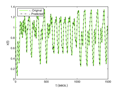
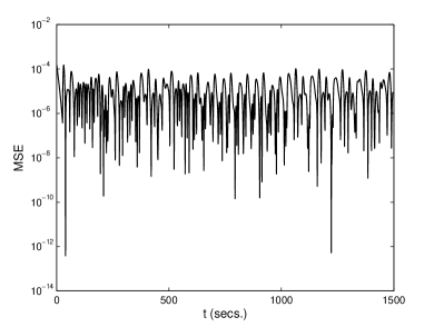
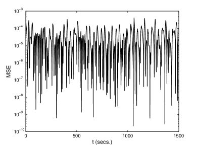
where, secs. Here, . Integration with a fourth-order Runge-Kutta routine yields the original solutions. The value of the embedding dimension is . The total number of points in the original solution is . The procedures described in Sections 2 and 3 are then employed for secs. to obtain , for . These results and the concomitant MSE values are depicted in Figs. 1 and 2, respectively.
Here, Fig. 1 clearly demonstrates that the predicted results faithfully capture the dynamics embedded in the chaotic M-G time series’. Fig. 2 expectedly demonstrates a slight distortion of the predicted signal vis-á-vis the original signal, as a consequence of long-term forecasting. It may be argued that the number of coefficients is high and can forecast just about any signal. This argument is not only tenuous at best for the case of chaotic signals, but is also orthogonal to the very reason causing the choosing of such a high value of . Specifically, Section 1 explicitly discusses the possible singularity (or near-singularity) of the embedding matrix W. As stated therein, large number of lags, W can result in volatile forecasts owing to ill-conditioning. The M-G DDE in this example has a higher embedding dimension than other prominent models (such as the Lorenz, Hénon, etc.) (see, for eg. Ref. [3]), and thus the resulting W would be more prone to result in volatile forecasts. As is evidenced by Figs. 1 and 2, this is not the case and the forecasts are clearly accurate and stable.
It is noteworthy to mention that the coefficients obtained from the training data during the modeling phase, which form the basis on which further prediction is done over a much larger time period and data sample size (as compared to those in the modeling phase), are unique to the specific data set under consideration. Specifically, coefficients obtained from different data sets, for example the M-G DDE with a different value of the lag or another nonlinear dynamics model, yield erroneous predictions if applied to a data set which differs from the one(s) they were obtained from. This issue is the task on ongoing studies briefly described in Section 6 within the context of the results described in Sections 3 and 4, and will be presented elsewhere.
5.2 MIT-BIH arrhythmia database Record 207
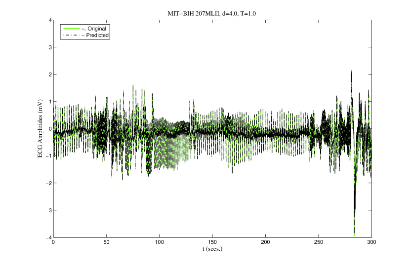
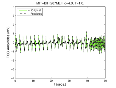
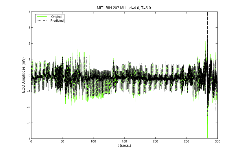
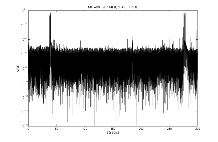
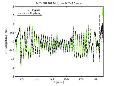
This sub-Section employs a 300 secs. (5min.) ECG signal to demonstrate that the model described in this paper accurately predicts episodes (transients) which are the artifacts of a diseased heart over a reasonable period of time, even for a highly erractic/volatile signal. The annotations are described in [62]. The signal is extracted from data obtained as a .mat data file from [63]. The sampling frequency of the data [64], the number of samples being for a total duration of . The rationale for the choice of 300 secs. sample is to ensure that the portion of the signal, both during the modeling phase and the prediction phase that follows, possess sufficiently identifiable episodes which are documented in the reference annotations [65]. It would be desirable to conduct the study over the entire duration of the signal spanning around 30 mins. However, this would yield simulation results that are visually incoherent, and hence the truncation of the signal length/duration. The number of training samples from which the values of is obtained is secs. for forecasting times of ( and (. In all cases, , , and . All simulation results are presented for the MLII lead. The simulation results depicting the predicted ECG signal superimposed over the original Record 207 signal for the MLII lead for T=1.0 and 5.0 respectively and the concomitant MSE’s are presented in Figs. 3 and 5, respectively.
Both Figs. (3) and (5) demonstrate that even for a relatively small duration of the modeling phase which comprises 1/6-th of the duration of the entire prediction exercise comprising of both the modeling phase and the prediction of new data, the prediction results are of a high quality. The case corresponding to shows greater ”undershoots” and ”overshoots” of the peaks of the signal as compared to the case of . This degradation of prediction performance is expected. The results of the MSE’s for both cases of the forecasting time shows divergent peaks. These have been analyzed and found to be the result of the highly erractic/volatile nature of the signal. It is important to note that they do not constitute any volatility in the prediction since the profiles of the predicted signals are demonstrated to be very much in accord with the original signal. Further, in both cases, following every divergent peak which can even be visually related to erratic signal quality in Figs. (3) and (5), the prediction returns to ”normalcy” which is defined by a low MSE value. This would not be the case of a volatile prediction cased by ill-conditioning or any other factor (see Section 1), because the errors cased by volatile predictions tend to cascade.
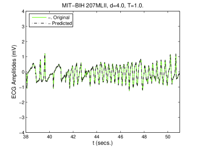
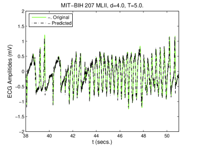
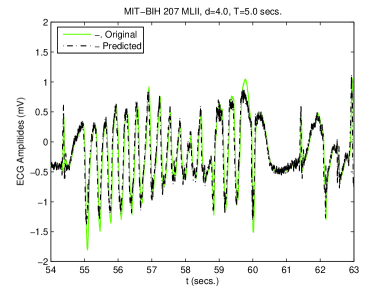
Figs. (4) and (6) focus on specific regions of interest. Figs. 4(a) and 6(a) depict the overlaid overlaid and predicted signals of the modeling phase for the cases of the forecasting time and , respectively. To establish the accuracy of the FIM based model, the prediction of the episodes corresponding to the various conditions of the diseased heart documented in the reference annotations [65], that can be visually determined in the period secs. are demonstrated in Figs. 4(b)-(d) and 6(b)-(d) for and , respectively. On inspection of Figs. 4(b) and 6(b), the instance of ventricular tachycardia identified by ”+” and defined by ”(VT” in the reference annotations at 38.522 secs., immediately followed by three instances of premature ventricular contraction identified by ”V” and the onset of ventricular flutter/fibrillation identified by ”[” at 40.736 secs. in the reference annotation followed by an instance of ventricular flutter identified by ”+” and defined by ”(VFL” in the reference annotations at 40.803 secs. and the subsequent termination of the ventricular flutter/fibrillation identified by ”]” at 50.972 secs. in the reference annotation can be easily identified. This region is of particular importance since it spans both the modeling phase from which the working hypothesis is determined from the training data, and the prediction of new data values.
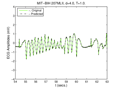
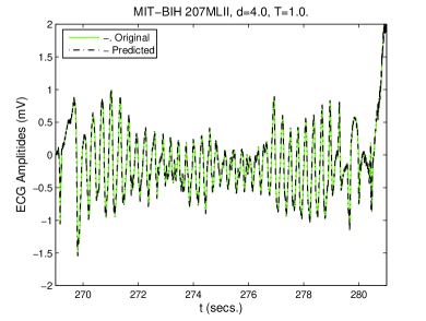
On inspection of Figs. 4(c) and 6(c), the onset of ventricular flutter/fibrillation identified by ”[” at 54.764 secs. in the reference annotation followed by an instance of ventricular flutter identified by ”+” and defined by ”(VFL” in the reference annotations at 54.869 secs. and the subsequent termination of the ventricular flutter/fibrillation identified by ”]” at 50.972 secs. in the reference annotation and the instance of ventricular tachycardia identified by ”+” and defined by ”(VT” in the reference annotations at 61.839 secs. (1:01.839 mins.), immediately followed by three instances of premature ventricular contraction identified by ”V”, can be easily identified. Finally, on inspection of Figs. 4(d) and 6(d), the onset of ventricular flutter/fibrillation identified by ”[” at 269.467 secs. (4:29.467 mins.) in the reference annotation followed by an instance of ventricular flutter identified by ”+” and defined by ”(VFL” in the reference annotations at 129.586 secs. (4:29.586 mins.) and the subsequent termination of the ventricular flutter/fibrillation identified by ”]” at 240.906 secs. (4:40.906 mins.) in the reference annotation, can be easily identified. In all cases depicted in Figs. (4) and (6), it is observed that the quality of the prediction is high, with the case of the example with being marginally degraded vis-á-vis the case with , which is expected.
5.3 Creighton University VTA database Record cudb/cu02
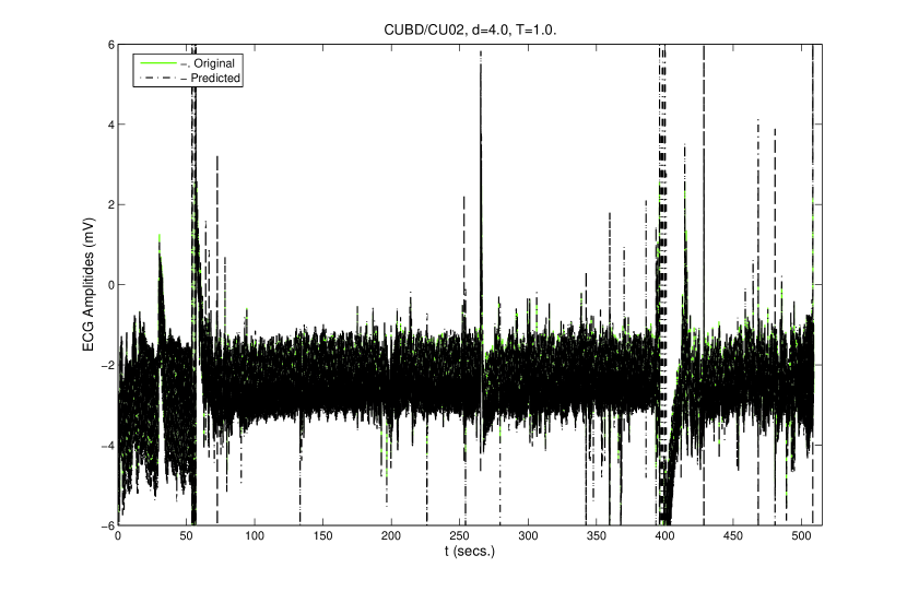
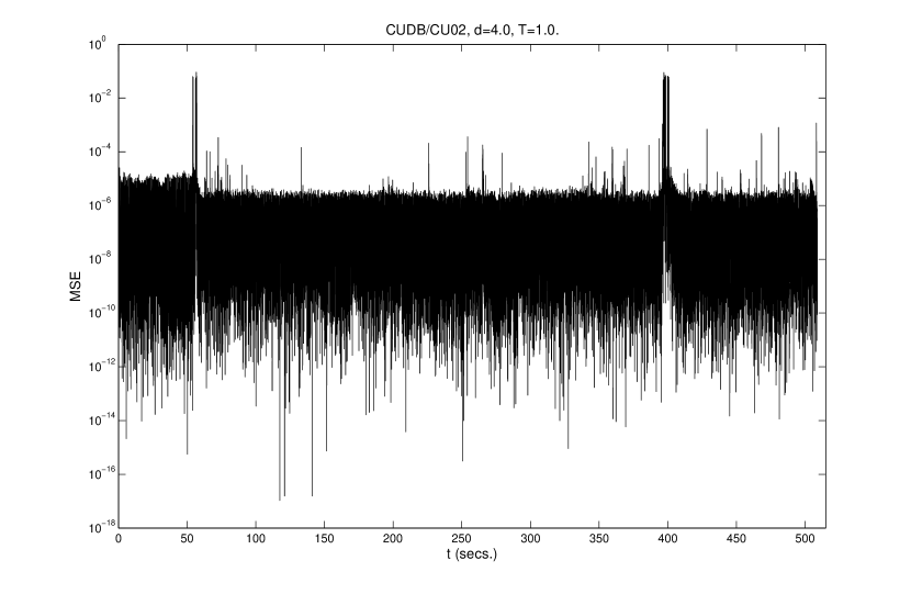
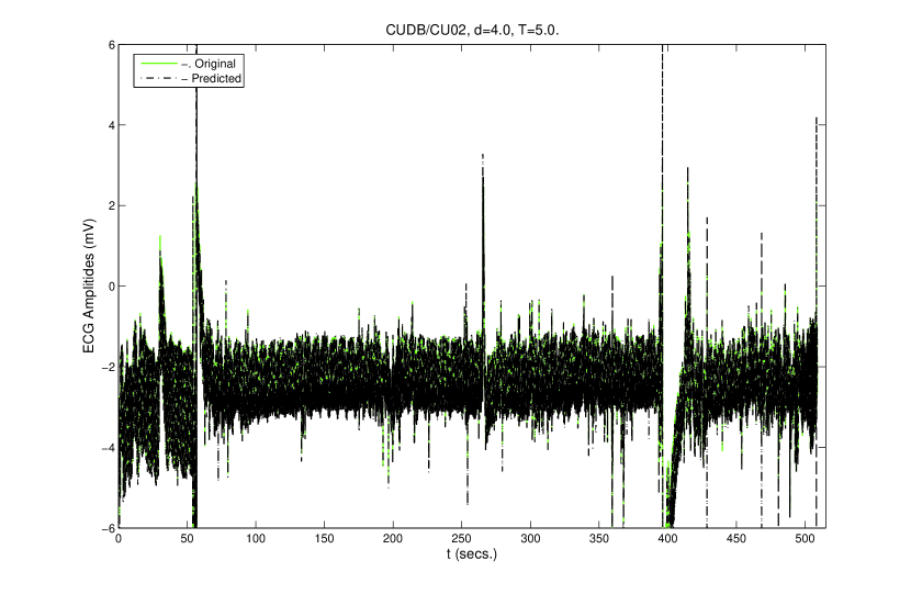
This sub-Section demonstrates the robustness of model described in this paper for an extended ECG signal, even for a highly erractic/volatile signal displaying the symptoms of cardiac VTA. The signal is extracted from data obtained as a .mat data file from [66]. The sampling frequency of the data , and the number of samples is , for a total duration of [67]. In order to study the robustness of the prediction performance of the FIM-based model, the number of training samples from which the values of is obtained is chosen to be secs. for ( and (. In all cases, , , and .
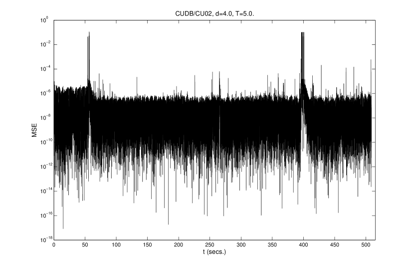
The high quality of the model is attested by the fidelity of the predicted ECG profiles with the original signals, and, the MSE’s. The simulation results depicting the predicted ECG signal superimposed over the original signal for T=1.0 and 5.0 and the concomitant MSE’s, are presented in Figs. 7 and 8, respectively. Similar to the case described in Section 5.2, the results of the MSE’s for both forecasting times depict divergent peaks. These have been analyzed and found to be the result of the nature of the signal. Again, note that these divergent peaks in the MSE’s do not constitute any volatility in the prediction since the profiles of the predicted signals are demonstrated to be very much in accord with the original signal. Further, in both cases, following every divergent peak which can even be visually related to erratic signal quality in Figs. (7) and (8), the prediction returns to ”normalcy” (defined by a low MSE value). This would not be the case in a volatile prediction cased by ill-conditioning or any other factor (see Section 1), because the errors cased by volatility of the forecasting tend to cascade.
6 Summary and conclusions
A convenient framework for the modeling and forecasting of time series has been developed within the ambit of a FIM-based inference model. The modeling phase from which the working hypothesis is derived has been provided with a QM connotation, by the formulation of a time independent Schrödinger-like equation in a vector setting, employing least squares constraints. This has been achieved by invoking the MFI principle. Apart from the obvious theoretical implications, this allows for the systematic derivation and categorization of the working hypothesis and the subsequential forecasting phase. The pdf and the pseudo-inverse relations have been self-consistently inferred by invoking the QM virial theorem for the case of normal distributions. The reciprocity relations and the LTS for the modeling phase have been derived for the modeling phase. This results in an intriguing form of the FIM for the modeling phase, which defines the working hypothesis, described solely in terms of the observed data (the empirical FIM).
The possible utilities of this form of the FIM are to derive principled expressions and values for the statistical dispersion. This FIM expression has no equivalent in prior MaxEnt models [7-10], which treat the statistical dispersion as an ad-hoc scaling [15]. The FIM-based model has been numerically tested, and its efficacy proven for the Mackey-Glass DDE, the ECG signal for the MLII lead from Record 207 of the MIT-BIH cardiac arrhythmia database, and the ECG from Record cudb/cuo2 of the Creighton University VTA database. The forecasting is consistently demonstrated to be of very high quality, and does not suffer from any signs of volatility caused by ill-conditioning of the embedding matrix W or any other factor. The numerical experiments on the ECG demonstrate that the model presented in this paper is able to forecast salient episodes documented in the reference annotations for the said signals, to a very high degree of accuracy. Ongoing work is focused on a two-pronged approach. First, the empirical FIM derived in Section 4 has been investigated within the context of its relationship to the FIM employed in Section 3, and the subsequent effects on the forecasting. A fiduciary time dependence is induced into the modeling phase via a sliding window analysis. This allows for the quality of prediction to be related to fundamental results governing the FIM, viz. the I-theorem (the Fisher-equivalent of the H-theorem) [24], for both normal and non-equilibrium distributions. Next, a principled comparison of the FIM-based model with existing nonparametric prediction models [12, 13] is in progress. These works will be presented elsewhere.
Appendix A: Derivation of Eq. (16)
For the Fisher information matrix , each element is defined by
| (A.1) |
For a possessing a-priori iid entries
| (A.2) |
Substituting (A.2) into (A.1) yields
| (A.3) |
For
| (A.4) |
since all other integrals integrate to unity because of normalization. For ,
| (A.5) |
Thus, is a diagonal matrix with each element defined by (A.5). Note that , as used in Eq. (16).
References
- [1] J.-P. Eckman, D. Ruelle, Rev. Mod. Phys. 15 (1985) 617-656.
- [2] H. D. I. Abarbanel, R. Brown, J. J. Sidorowich, L. Sh. Ysimring, Rev. Mod. Phys. 65 (1993) 1331-1392.
- [3] H. Kantz, T. Schreiber, Nonlinear Time Series Analysis, Cambridge Univ. Press, Cambridge U.K, 1999.
- [4] J. Rissanen, Ann. Stat. 14 (1989) 1080-1100.
- [5] F. Takens, ”Detecting strange attractors in turbulence”, in Dynamical Systems and Turbulence: Lecture Notes in Mathematics, Volume 898, Springer, Berlin, 1981, 366-381.
- [6] T. Sauer, J. A. Yorke, M. Casdagli, J. Stat. Phys. 65 (2000) 579.
- [7] L. Diambra, A. Plastino, Phys. Lett. A 216 (1996) 278-282.
- [8] M. T. Martín, A. Plastino, V. Vampa, G. Judge, Physica A 405 (2014) 63-69.
- [9] M. T. Martín, A. Plastino, V. Vampa, Entropy 16 (2014) 4603-4611.
- [10] A. F. Bariviera, M. T. Martín, A. Plastino, V. Vampa, Physica A 449 (2016) 401-407.
- [11] E. T. Jaynes, Phys. Rev. 106 (1957) 620-630.
- [12] J. C. Principe, Information Theoretic Learning - Renyi’s Entropy and Kernel Perspectives, Springer, New York, 2010.
- [13] W. Liu, J. C. Principe, S. Haykin, Kernel Adaptive Filtering : A Comprehensive Introduction, Wiley, Hoboken NJ, 2010.
- [14] H. D. I. Abarbanel, Analysis of Observed Chaotic Data, Springer, New York, 1996.
- [15] L. Diambra, Physica A 278 2000) 140-149.
- [16] N. Wiener. Extrapolation, Interpolation, and Smoothening of Stationary Time Series with Engineering Applications, Wiley, New York, 1949.
- [17] M. Casdagli, Physica D 35 (1989) 335-356.
- [18] J. C. Principe, A. Rathie, J.-M. Kuo, Intl. J. of Bifurcation and Chaos 2 1992 989-996.
- [19] D. Mandic, J. Chambers, Recurrent Neural Networks for Prediction, Wiley, Chichester, 2001.
- [20] L. Diambra, A. Plastino, Phys. Rev. E 52 (1995 4557-4560.
- [21] N. I. Sapankevych, R. Sankar, IEEE Comput. Intell. Mag., 4 (2009) 24-38.
- [22] J. P. Crutchfield, B. S. McNamara, Complex Systems, 21 (1985) 417.
- [23] J. D. Farmer, J. J. Sidorowich, Phys. Rev. Lett. 59 (1987) 845.
- [24] B. R. Frieden, Science from Fisher Information - A Unification, Cambridge University Press Cambridge, 2004.
- [25] J.A. Wheeler, in Zurek W. H. (Ed.): Complexity, Entropy and the Physics of Information, Addison Wesley, New York, 3-28, 1991.
- [26] P. J. Hüber, Robust Statistics, Wiley, Newy York, 1981.
- [27] B. R.Frieden, Phys. Rev. A, 41 (2000) 4265-4276; Optics Lett, 14 (1989) 199-201.
- [28] B. R. Frieden, A. Plastino, A. R. Plastino, B. H. Soffer, Phys. Rev. E 66 (2002) 046128.
- [29] B.R. Frieden, A. Plastino, A. R. Plastino, B. H. Soffer, Phys. Lett. A 304 (2002) 73-78.
- [30] J. S. Dehesa, Á. G. Martín, P. Sánchez-Moreno, Complex Anal. and Oper. Th. 6 (2012) 585-601.
- [31] W. Greiner, Quantum Mechanics. An Introduction, Springer, Berlin, 2012.
- [32] F. N. Fernandez and E. A. Castro, Hypervirial Theorems, Lecture Notes in Chemistry, Vol. 43, Springer-Verlag, Berlin, 1987.
- [33] R. C. Venkatesan, ”Statistical Cryptography using a Fisher-Schrödinger model”, Proc. IEEE Symposium on Foundations of Computational Intelligence (FOCI 2007), 487, IEEE Press, Piscataway, NJ, 2007.
- [34] R. C. Venkatesan, ”Encryption of Covert Information through a Fisher Game”, in Exploratory Data Analysis using Fisher Information, Frieden, B.R. and Gatenby, R.A., (Eds.), Springer- Verlag, London, 181-216, 2006.
- [35] B. R.Frieden, A. Plastino, A. R. Plastino, B. H. Soffer, Phys. Rev. E, 60 (1999) 046128.
- [36] S. P. Flego, A. Plastino, A. R. Plastino, Ann. Phys., 326 (2011) 2533-2543.
- [37] S. P. Flego, A. Plastino, A. R. Plastino, Physica A 390 (2011) 2276-2282.
- [38] S. P. Flego, A. Plastino, A. R. Plastino, Physica A 390 (2011) 4702-4712.
- [39] S. P. Flego, A. Plastino, A. R. Plastino, Physica Scripta, 85 (2012) 055002-055008.
- [40] C. Villani, Topics in Optimal Transportation, Graduate Studies in Mathematics Vol.58, American Mathematical Society, 2000.
- [41] G. Blower, Random Matrices: High Dimensional Phenomena, London Mathematical Society Lecture Notes, Cambridge University Press, Cambridge, 2009.
- [42] P. Zegers, Entropy 17 (2015) 4918-4939; B. R. Frieden, B. H. Soffer, Phys. Lett. A 374 (2010) 3895-3898.
- [43] R. C. Venkatesan, A. Plastino, Phys. Lett. A, 378 (2014) 1341-1345.
- [44] R. C. Venkatesan, A. Plastino, Ann. Phys., 359 (2015) 300-316.
- [45] S. M. Kay, Fundamentals of Statistical Signal Processing, Vol I: Estimation Theory, Prentice-Hall Signal Processing Series, 1993.
- [46] M. Casas, F. Pennini, A. Plastino, Phys. Lett. A 235 (1997) 457-463.
- [47] M.C.Mackey, L.Glass, Science 197 (1977) 287-289.
- [48] G. B. Moody, R. G. Mark, IEEE Eng. in Med and Biol. 20 (2001) 45-50.
- [49] F. M. Nolle, F. K. Badura, J. M. Catlett, R. W. Bowser, M. H. Sketch, ”CREI-GARD, a new concept in computerized arrhythmia monitoring systems”, Computers in Cardiology 1986 13, 515-518, IEEE Press, Piscataway, NJ, 1986.
- [50] A. L. Goldberger, L. A. N. Amaral, L. Glass, J. M. Hausdorff, P. Ch. Ivanov, R. G. Mark, J. E. Mietus, G. B. Moody, C.-K. Peng, H. E. Stanley, Circulation, 01(2000 e215-e220.
- [51] G. H. Golub, C. L. van Loan, Matrix Computations, third ed., Johns Hopkins Univ. Press, Baltimore, 1995.
- [52] L. Diambra, C. P. Malta, Phys. Rev. E 57 (1999) 929-937.
- [53] B. Pompe, ”Mutual Information and Relevant Variables for Predictions”, in Modeling and Forecasting Financial Data Techniques for Nonlinear Dynamics, Soofi, A. S. and Cao, L., (Eds.), Springer, New York, pp. 61-92, 2002.
- [54] A. B. Owen, Empirical Likelihood, Chapman & Hall/CRC, Boca Raton, 2001.
- [55] D. Guo, S. Shamai (Shitz) and S. Verdú, The Interplay Between Information and Estimation Measures, Foundations and Trends in Signal Processing Ser., Now Publishers, Boston, 2012.
- [56] M. Casas, A. Plastino, A. Puente, Phys. Lett. A 248 (1998) 161-166.
- [57] M. Kennel, R. Brown, H. D. I. Abarbanel, Phys. Rev. A;45 (1992) 3403-3411.
- [58] P. I. Grassberger, I. Procaccia, Physica D, 9 (1983) 189-208.
- [59] J. D. Farmer, Physica D, 4 (1982)366-393.
- [60] R. B. Govindan, K. Narayanan, M. S. Gopinathan, Chaos, 8 (1998) 495-502.
- [61] A. Casaleggio, S. Braiotta,”Study of the Lyapunov exponents of ECG signals from MIT-BIH database”, Computers in Cardiology 1995, 697-700. IEEE Press, Piscataway, NJ, 1995; A. Casaleggio, S.Braiotta, Chaos Sol. & Frac., 9 (1997) 1591-1599.
- [62] https://physionet.org/physiobank/annotations.shtml
- [63] https://physionet.org/atm/mitdb/207/atr/0/3600/export/matlab/207m.mat
- [64] https://physionet.org/atm/mitdb/207/description/record.txt
- [65] https://physionet.org/atm/mitdb/207/atr/0/3600/rdann/annotations.txt
- [66] https://physionet.org/atm/cudb/cu02/atr/0/3600/export/matlab/cu02m.mat
- [67] https://physionet.org/atm/cudb/cu02/description/record.txt
