Flavor structure, Higgs boson mass and dark matter in supersymmetric model with vector-like generations

Abstract

We study a supersymmetric model in which the Higgs mass, the muon anomalous magnetic moment and the dark matter are simultaneously explained with extra vector-like generation multiplets. For the explanations, non-trivial flavor structures and a singlet field are required. In this paper, we study the flavor texture by using the Froggatt-Nielsen mechanism, and then find realistic flavor structures which reproduce the Cabbibo-Kobayashi-Maskawa matrix and fermion masses at low energy. Furthermore, we find that the fermion component of the singlet field becomes a good candidate of dark matter. In our model, flavor physics and dark matter are explained with moderate size couplings through renormalization group flows, and the presence of dark matter supports the existence of just three generations in low energy scales. We analyze the parameter region where the current thermal relic abundance of dark matter, the Higgs boson mass and the muon $g-2$ can be explained simultaneously.

1 Introduction

The discovery of the Higgs boson by ATLAS and CMS collaborations of the LHC gives big impact on particle physics [1]. At the experiment, the Higgs mass is confirmed to be $m_{h}^{2}=125.09\pm 0.21({\rm stat.})\pm 0.11({\rm syst.})\,{\rm GeV}$ [2]. By the discovery, the particles predicted by the Standard Model (SM) are experimentally confirmed. However, there still remains various problems to be solved beyond the SM. Among them, we focus on the muon anomalous magnetic moment (muon $g-2$) and dark matter (DM) in this paper. We reveal that flavor structures are important for the issues.

Experimentally, the muon $g-2$ is reported with $\Delta a_{\mu}=(26.1\pm 8.0)\times 10^{-10}$ [3, 4]. For the explanation of this result, the extension of the SM is a possibility. In [5], one of the present authors (M.N.) showed that the supersymmetric model with vector-like generations explains experimental results. In the analysis, the authors solved the renormalization group (RG) flow of the Yukawa matrices, and then found that a certain flavor structure of the quark and lepton sectors are required for the explanation of the muon $g-2$ and the Higgs mass. Further, in the model, a singlet scalar field is required to give large masses to the vector-like generations enough to avoid electroweak precise measurements [6]. In this paper, we show that the Yukawa structure is determined by the Froggatt-Nielsen mechanism, and the single field is a good candidate of the DM.

By astrophysical observations such as the Galaxy rotation curves [7], collisions of bullet clusters [8], or Cosmic Microwave Background [9], it is confirmed that the matter contents of the present Universe is mainly dominated by DM with the abundance $\Omega_{\rm DM}h^{2}=0.1198\pm 0.0015$ [9]. The formation of large scale structures also requires DM since it is a significant source of gravitational potential. However, there does not exist a natural candidate of DM in the SM. Thus, the extension of particle contents is needed. In our model, the superpartner of the singlet scalar field, which is called singlino, is the lightest supersymmetric particle (LSP), and it could be DM in the presence of R-parity. We show that the thermal relic abundance of the singlino field explains the DM abundance.

Another issue relevant to this paper is the origin of the flavor structure in the quark and lepton sectors. As in the case of the Cabbibo-Kobayashi-Maskawa (CKM) matrix in the SM, our model [5] needs Yukawa structures for the mass matrices of the quark and lepton sectors extended with vector-like generations. Especially, there should exist an appropriate flavor structure for explaining experimental values of both the Higgs mass and the muon $g-2$ through quantum corrections simultaneously. However, as in the SM, Yukawa couplings are just free parameters. We try to explain the structure by the Froggatt-Nielsen (FN) mechanism.

Froggatt and Nielsen explained the structure by assuming additional $U(1)$ symmetry called flavor symmetry [10]. The mechanism is realized also in SUSY models [11]. In this work, we reproduce the flavor structure of the model [5] by the FN mechanism. Then we show a charge assignment to the chiral superfields for realizing a realistic Yukawa hierarchy, which explains the CKM matrix and fermion masses at low energy with the parameter $\epsilon\simeq 0.33$. Here, $\epsilon$ is the breaking scale of FN U(1) symmetry normalized by the cutoff scale.

With an appropriate assignment of the FN charge, a SM singlet superfield $\Phi$ plays two important roles. One is to fix the mass scales of vector-like generations with the vacuum expectation value (VEV) of the scalar field $\langle\Phi\rangle$. Another is its fermion component becomes a candidate of DM with $R$-parity. In this sense, the presence of the DM supports the existence of three generations in low energy scales within our model. As seen later, we show a parameter space where one obtains the right amount of the Higgs boson mass, the muon $g-2$, and the observed relic abundance of DM in our model.

The organization of this paper is as follows. In Section 2, we introduce our model with the flavor symmetric superpotential. We assign the U(1) charge to each field and give possible Yukawa structure in both quark and lepton sectors. Then the observed CKM matrix and fermion masses can be reproduced at the $M_{Z}$ scale. Here, $M_{Z}\simeq 91$ GeV [12] is the $Z$ boson mass. In Section 3, we shall explain a candidate of DM in our model. Next, we give analytic equation for calculating the thermal relic abundance of the DM. In Section 4, we show the parameter region where the DM abundance, Higgs boson mass and the muon $g-2$ within $2\sigma$ level are simultaneously explained. The final section is devoted to the conclusion and discussion.

2 Model

In this section, we first give an explanation of the model proposed in [5]. Second, we extend the model by adding a $U(1)$ flavor symmetry with the FN mechanism [10, 11], and then show that a nontrivial flavor structure is obtained through the symmetry breaking with an appropriate charge assignment. Sizable couplings between the supersymmetric SM sector and vector-like generations significantly contribute to the Higgs boson mass and the muon $g-2$.

The original model is a extension of minimal supersymmetric standard model (MSSM) by adding a pair of vector-like generations and a SM singlet field $\Phi$ [5]. We assume that the Kähler potential is canonical. As usual, the superfields of the MSSM sector are given by

$$Q_{i},\;u_{i},\;d_{i},\;L_{i},\;e_{i},\quad(i=1,\cdots,3),$$ (2.1)

$$H_{u},\;H_{d},$$ (2.2)

where $Q_{i}$ and $L_{i}$ are the SU(2) doublets of quarks and leptons, $u_{i},d_{i}$ and $e_{i}$ are the SU(2) singlets of up-type, down-type quarks and charged leptons, respectively. The Higgs doublets are denoted by $H_{u}$ and $H_{d}$. In addition to these, we have other superfields of the vector-like generations and a singlet as

$$Q_{4},\;u_{4},\;d_{4},\;L_{4},\;e_{4},$$ (2.3)

$$\bar{Q},\;\bar{u},\;\bar{d},\;\bar{L},\;\bar{e},$$ (2.4)

$$\Phi.$$ (2.5)

The quantum charges of these superfields are summarized in Table 2.1. The superfields of fourth generation in (2.3) have the same charges as those of matters in the MSSM, while those of fifth in (2.4) have the opposite ones. These pairs with opposite charges are called vector-like generations. The fields $\Phi$ is a SM gauge singlet field, and its vacuum expectation value gives mass scales of the vector-like generations. With these superfields, the Yukawa sector of the superpotential is written as [5]

$$W =\sum_{i,j=1,\cdots,4}\Big{(}(y_{u})_{ij}u_{i}Q_{j}H_{u}+(y_{d})_{ij}d_{i}Q_{j}H_{d}+(y_{e})_{ij}e_{i}L_{j}H_{d}\Big{)}$$

$$\hskip 56.9055pt+y_{\bar{u}}\bar{u}\bar{Q}H_{d}+y_{\bar{d}}\bar{d}\bar{Q}H_{u}+y_{\bar{e}}\bar{e}\bar{L}H_{u}$$

$$\quad+\sum_{i=1,\cdots,4}\Big{(}y_{Q_{i}}\Phi Q_{i}\bar{Q}+y_{u_{i}}\Phi u_{i}\bar{u}+y_{d_{i}}\Phi d_{i}\bar{d}+y_{L_{i}}\Phi L_{i}\bar{L}+y_{e_{i}}\Phi e_{i}\bar{e}\Big{)}$$

$$\hskip 56.9055pt+y\Phi^{3},$$ (2.6)

where $y$’s are dimensionless couplings for each generation of quark and lepton sectors.Each term of the interactions contributes to experimental results of the muon $g-2$, the Higgs mass and DM abundance as explained below. The Yukawa couplings in the first line give the flavor structure in the SM sector on top of the fourth generation matter, and they largely contribute to the flavor physics, i.e., the muon $g-2$ [5]. The second line shows the coupling of the fifth generations to the Higgs fields, and these interactions do not crucially contribute to the flavor structure in the SM sector but do to the muon $g-2$ in our model. The third line shows the coupling of vector-like generations to the SM singlet field $\Phi$. After the symmetry breaking of the scalar component of $\Phi$, the vector-like generations obtain each mass from these terms. Further, owing to these terms, the lower experimental bounds on the mass of vector-like generations are avoided. In our model, the fermion component of $\Phi$ is a DM candidate whose mass is given by the last term $y\Phi^{3}$. We explain such structures by the FN mechanism.

The FN mechanism requires an additional SM singlet scalar field and it is supposed that the singlet field has interactions with quark and lepton sectors [10]. Then, the effective Yukawa couplings are determined through the interactions by the singlet VEV. The magnitude of the couplings are controlled by an assignment of the FN charge to the quark and lepton sectors. We apply this mechanism to our model by introducing a SM singlet superfield

$$\Theta.$$ (2.7)

Let us consider an example of the interaction based on FN charge with $W=(\Theta/\Lambda)^{n}u_{1}Q_{1}H_{u}$, where $n$ is an integer and $\Lambda$ is a cut off scale. Here we take the scale to $\Lambda\simeq 10^{16}{\rm GeV}$. Under an assignment of the FN $U(1)$ charge, the integer $n$ is determined to satisfy $nq(\Theta)+q(u_{1})+q(Q_{1})+q(H_{u})=0$, where $q(\Theta),~{}q(Q_{1}),~{}q(u_{1}),~{}$and $q(H_{u})$ are $U(1)$ charges of respective fields. With this integer, the VEV such that $\braket{\Theta}\neq 0<\Lambda$ makes the effective Yukawa couplings as $(y_{u})_{11}\propto(\braket{\Theta}/\Lambda)^{n}$. By this way, the Yukawa structures of the quarks and leptons are determined.

Using the FN mechanism, we extend the Yukawa interaction part (2.6). We assign the FN U(1) charge to the FN field $\Theta$ as

$$q(\Theta)=-1.$$ (2.8)

Together with the charge assignment exhibited in Table 2.1, the Yukawa sector of the superpotential is written as

$$W =\sum_{i,j=1,\cdots,4}\Big{(}(Y_{u})_{ij}\left(\frac{\Theta}{\Lambda}\right)^{n_{u}^{ij}}u_{i}Q_{j}H_{u}+(Y_{d})_{ij}\left(\frac{\Theta}{\Lambda}\right)^{n_{d}^{ij}}d_{i}Q_{j}H_{d}+(Y_{e})_{ij}\left(\frac{\Theta}{\Lambda}\right)^{n_{e}^{ij}}e_{i}L_{j}H_{d}\Big{)}$$

$$\hskip 56.9055pt+Y_{\bar{u}}\left(\frac{\Theta}{\Lambda}\right)^{n_{\bar{u}}}\bar{u}\bar{Q}H_{d}+Y_{\bar{d}}\left(\frac{\Theta}{\Lambda}\right)^{n_{\bar{d}}}\bar{d}\bar{Q}H_{u}+Y_{\bar{e}}\left(\frac{\Theta}{\Lambda}\right)^{n_{\bar{e}}}\bar{e}\bar{L}H_{u}$$

$$\quad+\sum_{i=1,\cdots,4}\Big{(}Y_{Q_{i}}\left(\frac{\Theta}{\Lambda}\right)^{n_{Q_{i}}}\Phi Q_{i}\bar{Q}+Y_{u_{i}}\left(\frac{\Theta}{\Lambda}\right)^{n_{u_{i}}}\Phi u_{i}\bar{u}+Y_{d_{i}}\left(\frac{\Theta}{\Lambda}\right)^{n_{d_{i}}}\Phi d_{i}\bar{d}$$

$$\hskip 56.9055pt+Y_{L_{i}}\left(\frac{\Theta}{\Lambda}\right)^{n_{L_{i}}}\Phi L_{i}\bar{L}+Y_{e_{i}}\left(\frac{\Theta}{\Lambda}\right)^{n_{e_{i}}}\Phi e_{i}\bar{e}\Big{)}+Y\left(\frac{\Theta}{\Lambda}\right)^{n_{\Phi}}\Phi^{3},$$ (2.9)

where magnitude of all Yukawa couplings is assumed to be of $\mathcal{O}(1)$. As explained, each power of $\Theta/\Lambda$ is determined from the charge assignment as

$$n_{u}^{ij} =q(u_{i})+q(Q_{j})+q(H_{u}),\ n_{d}^{ij}=q(d_{i})+q(Q_{j})+q(H_{d}),\ n_{e}^{ij}=q(e_{i})+q(L_{j})+q(H_{d}),$$

$$n_{\bar{u}} =q(\bar{u})+q(\bar{Q})+q(H_{d}),\ n_{\bar{d}}=q(\bar{d})+q(\bar{Q})+q(H_{u}),\ n_{\bar{e}}=q(\bar{e})+q(\bar{L})+q(H_{u}),$$

$$n_{Q_{i}} =q(Q_{i})+q(\bar{Q})+q(\Phi),\ n_{u_{i}}=q(u_{i})+q(\bar{u})+q(\Phi),\ n_{d_{i}}=q(d_{i})+q(\bar{d})+q(\Phi),\$$

$$n_{L_{i}} =q(L_{i})+q(\bar{L})+q(\Phi),\ n_{e_{i}}=q(e_{i})+q(\bar{e})+q(\Phi),\ n_{\Phi}=3q(\Phi).$$ (2.10)

Then, by the superpotential (2.9), the effective Yukawa couplings are given by

$$y_{x}\equiv Y_{x}\left(\frac{\braket{\Theta}}{\Lambda}\right)^{n_{x}},$$ (2.11)

where $x$ represents each generation of quark or lepton sectors. Note that with present charge assignment the cubic coefficient is same as $y=Y$ because of $q(\Phi)=0$. In this paper, we assume that the $U(1)_{\rm FN}$ is a gauged symmetry. With the D-term, the FN field obtains vacuum expectation value, but in this case, anomalies due to the symmetry could exist. Here let us comment about these issues. The case of the global symmetry is discussed at the end of this section.

	$(\text{SU}(3),\,\text{SU}(2),\,\text{U}(1))$
$Q_{4}$	(${\bm{3}},\,{\bm{2}},\,\frac{1}{6})$
$u_{4}$	(${\bm{3}^{*}},\,{\bm{1}},\,\frac{-2}{3})$
$d_{4}$	(${\bm{3}}^{*},\,{\bm{1}},\,\frac{1}{3})$
$L_{4}$	(${\bm{1}},\,{\bm{2}},\,\frac{-1}{2})$
$e_{4}$	(${\bm{1}},\,{\bm{1}},\,1)$
$\bar{Q}\equiv\left(\begin{array}[]{c}(u_{5R})^{C}\\ (d_{5R})^{C}\end{array}\right)$	(${\bm{3}}^{*},\,{\bm{2}},\,\frac{-1}{6})$
$\bar{u}\equiv u_{5L}$	(${\bm{3}},\,{\bm{1}},\,\frac{2}{3})$
$\bar{d}\equiv d_{5L}$	(${\bm{3}},\,{\bm{1}},\,\frac{-1}{3})$
$\bar{L}\equiv\left(\begin{array}[]{c}(\nu_{5R})^{C}\\ (e_{5R})^{C}\end{array}\right)$	(${\bm{1}},\,{\bm{2}},\,\frac{1}{2})$
$\bar{e}\equiv e_{5L}$	(${\bm{1}},\,{\bm{1}},\,-1)$
$\Phi$	(${\bm{1}},\,{\bm{1}},\,0)$
$\Theta$	(${\bm{1}},\,{\bm{1}},\,0)$

Table 2.1: The chiral superfields and their quantum number under the SM gauge group.

	$Q_{1}$	$Q_{2}$	$Q_{3}$	$Q_{4}$	$\bar{Q}$	$u_{1}$	$u_{2}$	$u_{3}$	$u_{4}$	$\bar{u}$	$d_{1}$	$d_{2}$	$d_{3}$	$d_{4}$	$\bar{d}$
U(1)${}_{\text{FN}}$	5	2	0	-2	2	4	2	0	-2	2	4	4	1	-2	-2

	$L_{1}$	$L_{2}$	$L_{3}$	$L_{4}$	$\bar{L}$	$e_{1}$	$e_{2}$	$e_{3}$	$e_{4}$	$\bar{e}$	$H_{u}$	$H_{d}$	$\Phi$	$\Theta$
U(1)${}_{\text{FN}}$	4	1	0	-1	0	5	1	1	0	2	0	0	0	-1

Table 2.2: The list for FN charge of each field.

Now, the VEV of the FN field is given by the FI D-term of the anomalous $U(1)_{\rm FN}$. Under the charge assignment, U(1)_FN becomes anomalous in our model because of tr$(q)>0$, if there are not any additional chiral multiplets with negative U(1)_FN charges. In such cases, theory is ill-defined. Based on the string theory, however, such anomalies can be canceled by the gauged shift of string theoretic axions (or p-from potentials) [13], and Fayet-lliopoulos term is naturally induced in U(1)_FN D-term at one-loop level with $\xi\sim\left({\rm tr}(q)M_{\ast}^{2}\right)/(16\pi^{2})$ [14, 15]. (See also [16] for a review.) Here $M_{\ast}$ is the string scale. In this paper, we assume that only $\Theta$ develops VEV [17] in the presence of U(1)_FN D-term potential by $D\sim\xi-|\Theta|^{2}\sim 0$ and that U(1)_FN anomalies are cancel-led by shifts of (multiple) axions which are coupled to the SM gauge fields in the viewpoint of generalized Green-Schwarz mechanism. Then, the chiral superfield $\Theta$ will be eaten by the anomalous U(1)_FN vector superfield in a supersymmetric manner. They become massive around the cutoff scale, and hence we will neglect them and U(1)${}_{\text{FN}}$ $D$-term contribution to the SUSY breaking, and focus only on the VEV in the followings.

As explained above, the effective Yukawa couplings are determined by the charge assignment of FN $U(1)$ and $\braket{\Theta}$. Especially, the charge assignment determines the flavor structure of our model. We explain the strategy to determine the assignment. First, we require the superpotential homomorphic for $\Theta$ at a perturbative level. To satisfy this requirement, the power of $\Theta/\Lambda$ needs to be positive. Under this constraint, we determine the FN charge, paying attention to two points: mixing between second and fourth generations and masses of fourth and fifth generations. In our vector-like generations model, low energy flavor structure in the SM sector is finally determined by RG equations. By solving RG equations, the authors of [5] found that for the appropriate flavor structure of the SM, the mixing between the second and fourth generations needs to be large. Thus we have to determine the FN charge such that this large coupling is reproduced. Another point is about the couplings between fourth and fifth generations. From the experimental constraint at Large Hadron Collider (LHC), the masses of vector-like generations are required to be relatively large as $m_{{\rm q}_{4}}\gtrsim 800\,{\rm GeV}$ and $m_{{\rm l}_{4}}\gtrsim 100\,{\rm GeV}$[12]. Thus the FN charge needs to be chosen to achieve these large masses.

Paying attention to those points, we have determined the assignment of the FN charge shown in Table 2.2. We explicitly show the mass matrix of each sector under the assignment. Let us here define a parameter for the convenience of explanation as

$$\epsilon=\frac{\left<\Theta\right>}{\Lambda}.$$ (2.12)

With this parameter, the matrix elements of up-type quark mass $M_{u}$, down-type quark mass $M_{d}$ and charged lepton mass $M_{e}$ are given as

$$M_{u} \approx \bordermatrix{&u_{1R}&u_{2R}&u_{3R}&u_{4R}&u_{5R}\cr u_{1L}&\epsilon^{9}v_{u}&\epsilon^{7}v_{u}&\epsilon^{5}v_{u}&\epsilon^{3}v_{u}&\epsilon^{7}V\cr u_{2L}&\epsilon^{6}v_{u}&\epsilon^{4}v_{u}&\epsilon^{2}v_{u}&v_{u}&\epsilon^{4}V\cr u_{3L}&\epsilon^{4}v_{u}&\epsilon^{2}v_{u}&v_{u}&0&\epsilon^{2}V\cr u_{4L}&\epsilon^{2}v_{u}&v_{u}&0&0&V\cr u_{5L}&\epsilon^{6}V&\epsilon^{4}V&\epsilon^{2}V&V&\epsilon^{4}v_{d}\cr},$$ (2.13)

$$M_{d} \approx \bordermatrix{&d_{1R}&d_{2R}&d_{3R}&d_{4R}&d_{5R}\cr d_{1L}&\epsilon^{9}v_{d}&\epsilon^{9}v_{d}&\epsilon^{6}v_{d}&\epsilon^{3}v_{d}&\epsilon^{7}V\cr d_{2L}&\epsilon^{6}v_{d}&\epsilon^{6}v_{d}&\epsilon^{3}v_{d}&v_{d}&\epsilon^{4}V\cr d_{3L}&\epsilon^{4}v_{d}&\epsilon^{4}v_{d}&\epsilon^{1}v_{d}&0&\epsilon^{2}V\cr d_{4L}&\epsilon^{2}v_{d}&\epsilon^{2}v_{d}&0&0&V\cr d_{5L}&\epsilon^{6}V&\epsilon^{6}V&\epsilon^{3}V&V&\epsilon^{4}v_{u}\cr},$$ (2.14)

$$M_{e} \approx \bordermatrix{&e_{1R}&e_{2R}&e_{3R}&e_{4R}&e_{5R}\cr e_{1L}&\epsilon^{9}v_{d}&\epsilon^{5}v_{d}&\epsilon^{5}v_{d}&\epsilon^{4}v_{d}&\epsilon^{6}V\cr e_{2L}&\epsilon^{6}v_{d}&\epsilon^{2}v_{d}&\epsilon^{2}v_{d}&\epsilon^{1}v_{d}&\epsilon^{3}V\cr e_{3L}&\epsilon^{5}v_{d}&\epsilon^{1}v_{d}&\epsilon^{1}v_{d}&v_{d}&\epsilon^{2}V\cr e_{4L}&\epsilon^{4}v_{d}&v_{d}&v_{d}&0&\epsilon^{1}V\cr e_{5L}&\epsilon^{5}V&\epsilon^{1}V&\epsilon^{1}V&V&\epsilon^{2}v_{u}\cr},$$ (2.15)

where we neglected ${\cal O}(1)$ bare Yukawa couplings in the superpotential. Here we defined the vacuum expectation values of $H_{u},~{}H_{d}$ and $\Phi$ as

$$\braket{H_{u}}\equiv v_{u},~{}\braket{H_{d}}\equiv v_{d},~{}\braket{\Phi}\equiv V,$$ (2.16)

and defined the fermion components of $\bar{Q},~{}\bar{u}$ and $\bar{d}$ as

$$\left.\bar{Q}\right|_{\rm fermion}\equiv\left(\begin{matrix}(u_{5R})^{c}\\ (d_{5R})^{c}\end{matrix}\right),~{}\left.\bar{u}\right|_{\rm fermion}\equiv(u_{5L}),~{}\left.\bar{d}\right|_{\rm fermion}\equiv(d_{5L}).$$ (2.17)

As for three generations of the SM and fourth generations, the up-type Higgs $H_{u}$ couples to up-type quarks, and the down-type Higgs $H_{d}$ couples to down-type quarks and leptons in the Yukawa sector. (See the first line in Eq. (2.9).) These terms correspond to the $4\times 4$ parts of the mass matrices (2.13), (2.14) and (2.15). As for the fifth generations, the Higgs couples in the opposite way, that is, $H_{u}$ couples to down-type quark of fifth generation, and $H_{d}$ couples to up-type quark as shown in the fourth line in Eq. (2.9), which correspond to $5-5$ entry in the mass matrices. The other elements of the mass matrices are given by the gauge singlet field $\Phi$. (See the third and fourth lines in Eq. (2.9).)

Now we discuss about the observables of the CKM matrix and fermion masses in both quark and lepton sectors. In our model, the CKM matrix is extracted from $5\times 5$ unitary matrix. Thus we need to check carefully that the unitarity of the CKM matrix is satisfied so that the CKM matrix elements other than ordinary $3\times 3$ matrix are suppressed by the vector-like mass. The CKM matrix is defined by the part of the upper-left $3\times 3$ matrix of the product of $5\times 5$ unitary matrices:

$$(V_{\text{CKM}})_{ij}=(V_{uL}^{\dagger}V_{dL})_{ij}\hskip 8.53581pt(i,j=1,2,3),$$ (2.18)

where $i,j$ are generation labels.

$\epsilon$	$\alpha_{\rm GUT}$	$M_{\rm GUT}$ = $\Lambda$	$M_{\rm SUSY}$	$V$	$\tan\beta$
0.33	0.10	$6.0\times 10^{16}$ GeV	5.0 TeV	2.0 TeV	40

Table 2.3: The set of input values.

up-type quark Yukawa	down-type quark Yukawa	charged lepton Yukawa
$(Y_{u})_{11}$ = 2.000	$(Y_{d})_{11}$ = 0.500	$(Y_{e})_{14}$ = 2.000
$(Y_{u})_{23}$ = 2.000	$(Y_{d})_{21}$ = 1.930	$(Y_{e})_{12}$ = 2.000
$(Y_{u})_{33}$ = 2.000	$(Y_{d})_{22}$ = 1.200	$(Y_{e})_{21}$ = 2.000
$(Y_{u})_{41}$ = 0.500	$(Y_{d})_{23}$ = 0.900	$(Y_{e})_{22}$ = 0.500
$Y_{u_{3}}$ = 2.000	$(Y_{d})_{31}$ = 0.632	$(Y_{e})_{24}$ = 2.000
	$(Y_{d})_{32}$ = 0.700	$(Y_{e})_{34}$ = 0.500
	$(Y_{d})_{33}$ = 2.000	${Y}_{41}$ = 2.000
	$(Y_{d})_{41}$ = 2.000	${Y}_{42}$ = 2.000
	$Y_{d_{2}}$ = 1.100	${Y}_{L_{2}}$ = 2.000
		${Y}_{L_{3}}$ = 0.500
		${Y}_{L_{4}}$ = 0.500
		${Y}_{e_{2}}$ = 0.500
		${Y}_{e_{3}}$ = 2.000
		${Y}_{\bar{e}}$ = 2.000

Table 2.4: The set of input values for coupling constants in Eq. (2.9). Other coupling constants which are not written in this table are set to be unity. Note that all couplings are of ${\cal O}(1)$.

These $5\times 5$ unitary matrices diagonalize the up-type and down-type quark mass matrices:

$$V_{uR}M_{u}V_{uL}^{\dagger},$$ (2.19)

$$V_{dR}M_{d}V_{dL}^{\dagger}.$$ (2.20)

With the structures of the mass matrices (2.13), (2.14) and (2.15), we solve the RG equations. The input parameters for the equation are summarized in Table 2.4 and 2.4. By the calculation, we have confirmed that the CKM matrix and fermion masses at the $M_{Z}$ scale reproduce the observed ones. The RG equations in our model are listed in Appendix D. In Table 2.4, $\alpha_{\text{GUT}}$ and $\Lambda$ are the initial condition of RG equations for the MSSM gauge couplings obtained in [5]. It is found that the MSSM gauge couplings unify at a certain scale $M_{\text{GUT}}$ which is slightly high compared to the MSSM without vector-like generations. Thus, we use these values as boundary conditions for RG running. The scale $M_{\text{SUSY}}$ is a typical threshold for supersymmetric particles, and the ratio of the vacuum expectation values of Higgs doublets is defined as $\tan\beta\equiv v_{u}/v_{d}$. In Section 4, we use the same input values for the numerical analysis of the DM abundance, the Higgs boson mass and the muon $g-2$. Here, as an example, we show the result of RG running for the Yukawa couplings of the third generation in Fig. 2.1. The horizontal axis is energy scale, and the vertical axis is the strength of the Yukawa couplings. The blue, black and red lines correspond to the RG running of $(y_{u})_{33}$, $(y_{d})_{33}$ and $(y_{e})_{33}$, respectively. In the Fig. 2.1, each Yukawa coupling converges to a certain value at low energy, where these couplings do not depend on the initial values at $M_{\text{GUT}}$. The detailed analysis for the convergecy of Yukawa couplings are performed in [21]. As for $(y_{d})_{33}$, it seems that this Yukawa coupling does not evolve, but the initial value of $(y_{d})_{33}$ just coincides with the infrared value.

Figure 2.1: The result of RG running for the Yukawa couplings of the third generation. Horizontal axis is energy scale and vertical axis is the strength of the Yukawa couplings. Blue, black and red line correspond to the RG running of $(y_{u})_{33}$, $(y_{d})_{33}$ and $(y_{e})_{33}$, respectively.

Such RG runnings reproduce the fermion masses and the CKM matrix at the scale of $M_{Z}$:

$$m_{t}\sim 170\ \text{GeV},\hskip 8.53581ptm_{c}\sim 0.7\ \text{GeV},\hskip 8.53581ptm_{u}\sim 5.0\ \text{MeV},$$

$$m_{b}\sim 3.0\ \text{GeV},\hskip 8.53581ptm_{s}\sim 0.032\ \text{GeV},\hskip 8.53581ptm_{d}\sim 1.0\ \text{MeV},$$

$$m_{\tau}\sim 1.6\ \text{GeV},\hskip 8.53581ptm_{\mu}\sim 0.10\ \text{GeV},\hskip 8.53581ptm_{e}\sim 0.2\ \text{MeV},$$ (2.21)

$$|V_{\text{CKM}}|\sim\left(\begin{array}[]{ccc}0.974&0.226&0.0035\\ 0.225&0.973&0.040\\ 0.0089&0.041&0.999.\end{array}\right).$$ (2.25)

Fermion masses at the $M_{Z}$ scale are studied in [22], and the CKM matrix takes its value within 2$\sigma$ level of observed CKM matrix [12] as

$$\left(\begin{array}[]{ccc}0.97403-0.97449&0.22406-0.22606&0.00327-0.00387\\ 0.22392-0.22592&0.97325-0.97377&0.04084-0.04136\\ 0.00815-0.00939&0.0377-0.0429&0.9991-0.9992\end{array}\right).$$ (2.29)

These are consistent with Eq. (2.21) and (2.25).

Here let us discuss the case that the FN symmetry is global. In this case, there exists a (pseudo) NG boson associated with the spontaneous symmetry breaking of $U(1)_{\rm FN}$. We call it FN axion. As in the case of the QCD-axion, this FN axion could be another DM candidate. Further, it has interactions with the quarks and leptons, and through the anomaly effects it couples to gluons and electric-magnetic fields with an effective decay rates. The interactions give experimental and cosmological constraints on the VEV of FN field [23]. In the basis that the mass matrices of quarks and leptons are diagonalized, the Yukawa interactions are written by

$$-{\cal L}=\sum_{f=u,d,l}\left[m_{i}^{f}\bar{f}_{Li}^{{}^{\prime}}f^{\prime}_{R_{i}}+\kappa_{ij}^{f}\frac{s+ia}{\sqrt{2}v_{\Theta}}\bar{f}_{Li}^{{}^{\prime}}f^{\prime}_{R_{j}}\right],$$ (2.30)

where the coupling $\kappa^{f}_{ij}$ is determined by the mass matrix of fermions and FN charge as

$$\kappa_{ij}^{f}\equiv\left(V^{f_{L}+}\right)_{ik}\left(M_{kn}^{f}n_{kn}^{f}\right)V^{f_{R}}_{nj}.$$ (2.31)

Here we have expanded the FN field around the VEV as

$$\Theta=v_{\Theta}+\frac{s+ia}{\sqrt{2}}.$$ (2.32)

Thus, the interactions of the axion with quarks and leptons are given by

$$-{\cal L}_{\rm int}=\frac{ia}{\sqrt{2}v_{\Theta}}\sum_{f=u^{\prime},d^{\prime},l^{\prime}}\left[\left(\kappa_{H}^{f}\right)_{ij}\bar{f}_{i}\gamma_{5}f_{j}+\left(\kappa_{A}^{f}\right)_{ij}\bar{f}_{i}f_{j}\right],$$ (2.33)

where we have redefined the coupling of axion as

$$\left\{\begin{split}\left(\kappa^{f}_{H}\right)_{ij}&\equiv\frac{\left(\kappa^{f}+\kappa^{f\dagger}\right)_{ij}}{2},\\ \left(\kappa^{f}_{A}\right)_{ij}&\equiv\frac{\left(\kappa^{f}-\kappa^{f\dagger}\right)_{ij}}{2}.\end{split}\right.$$ (2.34)

Further, through the critical rotation as in the case of the QCD-axion, the axial interaction of the FN axion with gluons is given by

$$-{\cal L}_{{\rm gluon-axion}}=\frac{g_{s}^{2}}{32\pi^{2}}\left[\sum_{i=1...5;f=u,d}\frac{\left(\kappa_{H}^{f}\right)_{ii}}{m_{i}^{f}}\right]\frac{a}{\sqrt{2}v_{\Theta}}G_{\mu\nu}^{a}\tilde{G}^{\mu\nu a}=\frac{g_{s}^{2}}{32\pi^{2}}\frac{a}{f_{a}}G_{\mu\nu}^{a}\tilde{G}^{\mu\nu a},$$ (2.35)

where we have defined the domain wall number $N_{DW}$ and the effective decay constant $f_{a}$ as

$$N_{DW}\equiv\sum_{i=1...5;f=u,d}\frac{\left(\kappa_{H}^{f}\right)_{ii}}{m_{i}^{f}}={\rm tr}\left(n_{u}^{ij}+n_{d}^{ij}+n_{\bar{u}}+n_{\bar{d}}+n_{Q_{i}}+n_{u_{i}}+n_{d_{i}}\right),$$ (2.36)

and

$$f_{a}\equiv\frac{\sqrt{2}v_{\Theta}}{N_{DW}}.$$ (2.37)

Now, the domain wall number for our FN charge assignment is calculated as $N_{\rm DW}=54$. In our model, the effective decay constant is typically $f_{a}\simeq 10^{14}{\rm GeV}$. Among them, the interactions of the FN axion to the up type and down type quarks give a sizable contribution to the decay of the charged kaon via $K^{+}\rightarrow\pi^{+}a$. The decay rate for this process is evaluated by

$$\Gamma\left(K^{+}\rightarrow\pi^{+}a\right)=\frac{m_{K}^{3}}{32\pi v_{\Theta}^{2}}\left(1-\frac{m_{\pi}^{2}}{m_{K}^{2}}\right)^{3}\left|\frac{\left(\kappa_{A}^{d}\right)_{12}}{m_{s}-m_{d}}\right|.$$ (2.38)

The last term is of order unity as $\left(\kappa_{A}^{d}\right)_{12}=(3/2)\left(m_{s}-m_{d}\right)$. Thus, the branching ratio for this process is given by

$${\rm Br}\left(K^{+}\rightarrow\pi^{+}a\right)\simeq 10^{-11}\left(\frac{10^{11}{\rm GeV}}{v_{\Theta}}\right)^{2}.$$ (2.39)

With experimental bound ${\rm Br}(K^{+}\rightarrow\pi^{+}a)\lesssim 7.3\times 10^{-11}$ [24], we obtain a constraint

$$v_{\Theta}\gtrsim 10^{11}{\rm GeV}.$$ (2.40)

Through the interaction of the axion with quarks, the FN axion takes away the energy of the supernovae explosion. From the observation of the SM1987A by Kamiokande, this interaction is constrained in terms of the effective decay rate as $f_{a}\gtrsim 10^{9}{\rm GeV}$. With our definition for the effective decay rate, this constraint is reduced to

$$v_{\Theta}\gtrsim\frac{N_{DW}}{\sqrt{2}}10^{9}{\rm GeV}\sim 10^{10}{\rm GeV}.$$ (2.41)

Therefore, in the case that the FN $U(1)$ symmetry is global, the VEV of the FN field needs to be $v_{\Theta}\gtrsim 10^{11}{\rm GeV}$. As in the case of the QCD-axion, energy density of the coherent oscillation of this FN axion could explain the DM abundance given by [25]

$$\Omega_{a_{\Theta}}h^{2}=0.18\theta_{i}^{2}\left(\frac{f_{a}}{10^{12}{\rm GeV}}\right)^{1.19},$$ (2.42)

where $\theta_{i}$ is the initial misalignment of the FN axion $\theta_{i}\equiv a_{\Theta i}/f_{a}$. When the FN symmetry breaks, there could occur the formation of domain walls. We can assume that the breaking takes place before inflation. In this case, the domain wall problem is avoided, while in this case iso-curvature problem occurs. If the energy scale of inflation, that is, the Hubble parameter is small, this iso-curvature problem is avoided. The detail analysis and constraints on the parameters are studied in [23].

3 Dark matter

In this section, we calculate the abundance of thermal relics of a DM candidate, which is the fermion component of the singlet $\Phi$. The singlet superfield $\Phi$ is expanded as

$$\Phi=V+\theta\chi_{\Phi}+\cdots,$$ (3.1)

where $V$ is the VEV of the scalar component, $\chi_{\Phi}$ is the fermion component and $\theta$ is the fermionic coordinate on the superspace. In our model, the VEV of the singlet field $V$ gives masses to vector-like generations, and then experimental constraints on them at LHC are avoided.

First, we discuss the scale of the DM mass $m_{\chi_{\Phi}}$. In our model, the mass scale is determined by the VEV of $V$ and coupling constant of the cubic term $y~{}(=Y)$ as $m_{\chi_{\Phi}}=yV$. The RG running of $y$, whose RG equation is given in Eq. (D.35), is only governed by Yukawa couplings related to $\Phi$ and, it is insensitive to gauge sector. Thus, $y$ is pushed down to $\mathcal{O}(10^{-2})$ at low energy. With $V$ of a few TeV, $m_{\chi_{\Phi}}$ takes around $100\,{\rm GeV}$. This mass scale is smaller than other neutralino masses: bino and Higgsino masses. As for bino, its mass was studied in the previous study [5], and then it was revealed that the bino-like mass should be around $200\,{\rm GeV}$ to accord with the Higgs mass confirmed by the LHC. As for Higgsino-like neutralinos, those masses are determined from the electroweak symmetry breaking. In our model, we have assigned no FN charge to Higgs fields. Thus, in the superpotential, $H_{u}$ and $H_{d}$ have the so-called $\mu$ term as

$$W=\mu_{H}~{}H_{u}H_{d},$$ (3.2)

where $\mu_{H}$ is a constant of dimension unity. For the electroweak symmetry breaking, the mass parameter is required to $\mu_{H}\simeq 2\,{\rm TeV}$. Thus, the Higgsino-like neutralinos are heavier than the singlino. Therefore, $\chi_{\Phi}$ is the LSP in our model and could be a DM candidate because $R$-parity symmetry is imposed to our model. Let us comment on an operator $\Phi H_{u}H_{d}$ which can be written by gauge invariant in the superpotential. In this paper, we focus on $\Phi^{3}$ term in the superpotential because we would like to discuss the minimal model of $\chi_{\Phi}$, which does not couple to the Higgs sector. Such situation might be realized by imposing some symmetry.

In order to evaluate the DM abundance, we use the mass eigenstate basis for squarks, sleptons, quarks and charged leptons. For quark and lepton sectors, we diagonalize their mass matrices as

$$(V_{u_{R}}M_{u}V_{u_{L}}^{\dagger})_{ij} ={m_{U}}_{i}\delta_{ij},\hskip 14.22636pt(i,j=1,\dots,5)~{}\text{and}~{}(m_{U_{i}}<m_{U_{j}},~{}\text{if}~{}i<j),$$ (3.3)

$$(V_{d_{R}}M_{d}V_{d_{L}}^{\dagger})_{ij} ={m_{D}}_{i}\delta_{ij},\hskip 14.22636pt(i,j=1,\dots,5)~{}\text{and}~{}(m_{D_{i}}<m_{D_{j}},~{}\text{if}~{}i<j),$$ (3.4)

$$(V_{e_{R}}M_{e}V_{e_{L}}^{\dagger})_{ij} ={m_{E}}_{i}\delta_{ij},\hskip 14.22636pt(i,j=1,\dots,5)~{}\text{and}~{}(m_{E_{i}}<m_{E_{j}},~{}\text{if}~{}i<j).$$ (3.5)

We denote the mass eigenvalues $m_{U_{i}}$, $m_{D_{i}}$ and $m_{E_{i}}$ for the mass eigenstates of up-type quark ($U_{i}$), down-type quark ($D_{i}$) and charged lepton ($E_{i}$), respectively. As for squarks and charged slepton sectors, we also diagonalize their mass matrices as

$$(U_{\tilde{u}}M^{2}_{\tilde{u}}U_{\tilde{u}}^{\dagger})_{\alpha\beta} =m^{2}_{\tilde{U}_{\alpha}}\delta_{\alpha\beta},\hskip 14.22636pt(\alpha,\beta=1,\dots,10)~{}\text{and}~{}(m_{\tilde{U}_{\alpha}}^{2}<m_{\tilde{U}_{\beta}}^{2},~{}\text{if}~{}\alpha<\beta),$$ (3.6)

$$(U_{\tilde{d}}M^{2}_{\tilde{d}}U_{\tilde{d}}^{\dagger})_{\alpha\beta} =m^{2}_{\tilde{D}_{\alpha}}\delta_{\alpha\beta},\hskip 14.22636pt(\alpha,\beta=1,\dots,10)~{}\text{and}~{}(m_{\tilde{D}_{\alpha}}^{2}<m_{\tilde{D}_{\beta}}^{2},~{}\text{if}~{}\alpha<\beta),$$ (3.7)

$$(U_{\tilde{e}}M^{2}_{\tilde{e}}U_{\tilde{e}}^{\dagger})_{\alpha\beta} =m^{2}_{\tilde{E}_{\alpha}}\delta_{\alpha\beta},\hskip 14.22636pt(\alpha,\beta=1,\dots,10)~{}\text{and}~{}(m_{\tilde{E}_{\alpha}}^{2}<m_{\tilde{E}_{\beta}}^{2},~{}\text{if}~{}\alpha<\beta),$$ (3.8)

where $M_{\tilde{u}}^{2}$, $M_{\tilde{d}}^{2}$ and $M_{\tilde{e}}^{2}$ are up-type squark, down-type squark and charged slepton mass matrices defined in [5]. We denote the mass eigenvalues $m_{\tilde{U}_{\alpha}}^{2}$, $m_{\tilde{D}_{\alpha}}^{2}$ and $m_{\tilde{E}_{\alpha}}^{2}$ for the mass eigenstates of up-type squark ($\tilde{U}_{\alpha}$), down-type squark ($\tilde{D}_{\alpha}$) and charged slepton ($\tilde{E}_{\alpha}$), respectively.

The interaction terms of $\chi_{\Phi}$ can be read from the third to fourth line of Eq. (2.9). With the diagonalized basis in Eq. (3.3) $-$ (3.8), the interaction terms of $\chi_{\Phi}$ are given by

$$\mathcal{L} =\tilde{\bar{\chi}}_{\Phi}(O_{uRj\alpha}P_{R}+O_{uLj\alpha}P_{L})U_{j}\tilde{U}_{\alpha}^{*}+\tilde{\bar{\chi}}_{\Phi}(O_{dRj\alpha}P_{R}+O_{dLj\alpha}P_{L})D_{j}\tilde{D}_{\alpha}^{*}$$ (3.9)

$$+\tilde{\bar{\chi}}_{\Phi}(O_{eRj\alpha}P_{R}+O_{eLj\alpha}P_{L})E_{j}\tilde{E}_{\alpha}^{*}+{\rm h.c.},$$

where $P_{L}=(1-\gamma_{5})/2$, $P_{R}=(1+\gamma_{5})/2$ and coefficients are

$$O_{eRj\alpha} = (y_{e})_{i}(V_{eR})_{ji}(U_{\tilde{e}})_{\alpha 5},\hskip 8.53581ptO_{eLj\alpha}=(y_{L})_{i}(V_{eL})_{ji}(U_{\tilde{e}})_{\alpha 10},$$ (3.10)

$$O_{uRj\alpha} = (y_{u})_{i}(V_{uR})_{ji}(U_{\tilde{u}})_{\alpha 5},\hskip 8.53581ptO_{uLj\alpha}=(y_{Q})_{i}(V_{uL})_{ji}(U_{\tilde{u}})_{\alpha 10},$$ (3.11)

$$O_{dRj\alpha} = (y_{d})_{i}(V_{dR})_{ji}(U_{\tilde{d}})_{\alpha 5},\hskip 8.53581ptO_{dLj\alpha}=(y_{Q})_{i}(V_{dL})_{ji}(U_{\tilde{d}})_{\alpha 10},$$ (3.12)

The thermal abundance of the singlino DM is determined by their pair annihilation into the SM particles as shown in Fig. 3.1. This process ceases when the cosmic expansion rate drops bellow the annihilation rate:

$$\left<\sigma_{\text{ann}}v_{\text{rel}}\right>n_{\chi_{\Phi}}\simeq H(T_{\text{F}}),$$ (3.13)

where $\sigma_{\text{ann}}$ is the annihilation cross section, $v_{\text{rel}}$ is their relative velocity, $n_{\chi_{\Phi}}$ is the number density of $\chi_{\Phi}$ and $\left<...\right>$ represents thermal averaged cross section. We defined $T_{\rm F}$ as the freeze out temperature. After the freeze out, the number density of singlino drops at the same rate of the entropy density by the cosmic expansion. Thus, from Eq.(3.13), we can estimate the ratio of the number density to the entropy density at $T_{F}$ as :

$$\frac{n_{\chi_{\Phi}}}{s}\biggl{|}_{T_{\text{F}}}\simeq\frac{H(T_{\text{F}})}{\left<\sigma_{\text{ann}}v_{\text{rel}}\right>s}\biggl{|}_{T_{\text{F}}}=\frac{1}{4}\left(\frac{90}{\pi^{2}g_{*}(T_{\text{F}})}\right)^{1/2}\frac{1}{\left<\sigma_{\text{ann}}v_{\text{rel}}\right>T_{\text{F}}M_{\text{pl}}},$$ (3.14)

where $s$ is the entropy density, $g_{*}(T_{\text{F}})$ is the effective degrees of freedom of the radiation at the freeze-out and $M_{\text{pl}}=2.43\times 10^{18}$ GeV is the Planck mass.

Figure 3.1: The diagram of annihilation cross section for singlino DM. The left panel is the t channel process and the right panel is u channel process. $\chi_{\Phi}$ is singlino. $f_{i,j}$ ($f=U,D,E$) are the SM fermions whose masses are below freeze-out temperature $T_{\text{F}}$ So, we neglected top quark in the external lines. $\tilde{f}_{\alpha}$ ($\tilde{f}=\tilde{U},\tilde{D},\tilde{E}$) corresponds to mass eigenstate sfermions which are given in Eq. (3.9). The results of calculation for thermal averaged cross section are given in Appendix A.

The diagrams to calculate annihilation cross section are shown in Fig. 3.1, where $f_{i}$ is the SM fermion and $\tilde{f}_{\alpha}$ is sfermion exchanged in the process. Since the singlino is the SM gauge singlet and does not couple to the Higgs boson, the bosons do not appear in the process. The SM fermions entering in the process are the ones whose masses are bellow the freeze-out temperature $T_{\text{F}}$. In the calculation, one can expand $\left<\sigma_{\text{ann}}v_{\text{rel}}\right>=a+b/x_{\text{F}}+\mathcal{O}((1/x_{\text{F}})^{2})$ in the inverse of the power of $x_{\text{F}}\equiv m_{\chi_{\Phi}}/T_{\text{F}}$ and approximates $\left<\sigma_{\text{ann}}v_{\text{rel}}\right>$ by the coefficient $a$ and $b$. We take $x_{\text{F}}=20$ for the numerical analysis; $T_{F}$ becomes around 5 GeV for $m_{\chi_{\Phi}}=100$ GeV, and hence top quark contribution is neglected in the external lines. We calculate coefficient $a$ and $b$ for the case of Fig. 3.1 referring to [26]. The explicit forms of $a$ and $b$ are given in Appendix A. With the values of $x_{\text{F}}$, $a$ and $b$, the analytic form of the DM relic abundance is given by

$$\Omega_{\chi_{\Phi}}h^{2}\equiv\frac{\rho_{\chi_{\phi}}}{\rho_{c}/h^{2}}=\frac{m_{\chi_{\Phi}}n_{\chi_{\Phi}}/s}{\rho_{c}/(h^{2}s)} =\frac{1.07\times 10^{9}/\text{GeV}x_{\text{F}}}{\sqrt{g_{*}}M_{\text{Pl}}(a+b/x_{\text{F}})}\approx 0.1\times\left(\frac{8.0\times 10^{-9}\text{GeV}^{-2}}{\left<\sigma_{\text{ann}}v_{\text{rel}}\right>}\right),$$ (3.15)

where $h$ is the re-scaled Hubble constant, $\rho_{c}$ is the critical density of Universe, the ratio of critical density to the entropy density today is $\rho_{c}/s\simeq 1.8\times 10^{-9}$ GeV and we take $g_{*}(T_{F})=100$. In our model, the $p$-wave contribution is dominant to the thermal averaged cross section.

4 Higgs boson mass, muon $g-2$ and DM abundance

In this section, we show the results of numerical calculation for Higgs boson mass, the muon $g-2$ and the DM abundance. We have evaluated the Higgs boson mass and the muon $g-2$ at one-loop level. In this analysis, we determine the $\mu_{H}$ and $b$ terms in order that the electroweak symmetry breaking is triggered at Fermi scale. For the Higgs boson mass, we use the effective potential method [27] as usual for the MSSM case [28]. The quantum corrections to the Higgs mass from vector-like generations are calculated in the literature [29, 30]. In our model, the lightest Higgs boson mass $m_{h}^{2}$ is evaluated by

$$m_{h}^{2}=m_{h_{\text{tree}}}^{2}+\Delta m_{h}^{2},$$ (4.1)

where $m^{2}_{h_{\text{tree}}}=M_{Z}^{2}\cos^{2}(2\beta)$ and $\Delta m_{h}^{2}$ is one-loop corrections which are defined in Eq. (B.1). In the case of MSSM, the mass correction is mainly given by the stop field as $\Delta m_{h,~{}{\rm MSSM}}^{2}\simeq(3/4\pi^{2})y_{t}^{2}m_{t}^{2}\log(m_{\rm stop}^{2}/m_{t}^{2})$, but in our model the squark fields of the vector-like generation also give correction, and it is dominant. For the muon $g-2$, in our model, the one-loop contributions to the muon $g-2$ is given by

$$\Delta a_{\mu}=\Delta a_{\mu}^{\rm SUSY}+\Delta a_{\mu}^{\rm non-SUSY},$$ (4.2)

where $\Delta a_{\mu}^{\rm SUSY}$ and $\Delta a_{\mu}^{\rm non-SUSY}$ are SUSY contributions including both the MSSM [31] and vector-like [5] sector and non-SUSY contributions including only vector-like sector [32], respectively. $\Delta a_{\mu}^{\rm SUSY}$ and $\Delta a_{\mu}^{\rm non-SUSY}$ are defined in Eq. (B.16) and (B.34), respectively. The non-SUSY term is approximately given by the ratio of the muon mass to the charged lepton mass of the vector like generations as $\Delta a_{\mu}^{\rm non-SUSY}\simeq(\alpha/4\pi)~{}m_{\mu}^{2}/m_{L^{\prime}}^{2}$, where $\alpha$ is the fine structure constant of $SU(2)$ as $\alpha=g^{2}/(4\pi)$, and $m_{L^{\prime}}$ is the charged lepton mass of the vector-like generations. In addition to this term, in our model, the smuon, charged sleptons of the vector-like generations and their mixing in the mass matrix gives corrections to the muon $g-2$. Among of them, the charged leptons and sleptons of the vector-like generations gives sizable contributions. For the numerical calculation of the Higgs mass and the muon $g-2$, we have used Eq. (4.1) and Eq. (4.2).

As for the experiments, the current situation of the Higgs mass and muon $g-2$ are shown in the followings. The recent combined result of the Higgs boson mass $m_{h}^{\text{Exp}}$ reported by ATLAS and CMS collaborations [2] is given by

$$m_{h}^{\text{Exp}}=125.09\pm 0.21(\text{stat.})\pm 0.11(\text{syst.})~{}\text{GeV}.$$ (4.3)

The discrepancy of the muon $g-2$ between the SM predictions and experimental value is above $3\sigma$ and quantified as [3, 4]

$$\Delta a_{\mu}\equiv a_{\mu}(\text{Exp})-a_{\mu}(\text{SM})=(26.1\pm 8.0)\times 10^{-10}.$$ (4.4)

In the analysis, we assume the minimal gravity mediation [33] as the boundary condition of the SUSY-breaking scenario. In this scenario, there are five parameters: $m_{1/2},~{}m_{0},~{}A_{0},~{}\tan\beta$ and sigh of $\mu_{H}$. In this mediation model, we assume that the mass scale of gaugino, soft scalar and trilinear scalar coupling are universal respectively $m_{1/2},~{}m_{0},~{}A_{0}$ at the unification scale. $\tan\beta$ is fixed to reproduce the fermion masses at low energy and the sigh of $\mu_{H}$ is fixed plus so that the contributions to the muon $g-2$ become positive. Thus between the five parameters, there remain three free SUSY-breaking parameters: $m_{1/2}$, $m_{0}$ and $A_{0}$. In the following analysis, for the sake of simplicity, $A_{0}$ is fixed to be 0 GeV . In addition to the parameters of the minimal gravity mediation, our model have another parameter $y(=Y)$, which is exhibited in the superpotential (2.9) and is related to the DM mass. Yukawa couplings except for $y$ are determined so that the observed CKM matrix and fermion mass are reproduced. Since $y$ is insensitive to these observable, $y$ can be treated as a free parameter. After all, there are three parameters:

$$m_{1/2},\qquad m_{0},\qquad y.$$ (4.5)

In the analysis, we have calculated the Higgs boson mass at one-loop level. Inclusion of higher effects gives slight corrections for the mass. At two loop level, the Higgs mass correction in MSSM are studied such as in [34, 35, 36, 37, 38, 39, 40, 41, 42, 43]. The dominant contributions of the two-loop effects are from stop fields in loops by the superpotential

$$W=(y_{u})_{33}u_{3}Q_{3}H_{u}.$$ (4.6)

The amount of $\mathcal{O}(\alpha_{s}\alpha_{t})$ and $\mathcal{O}(\alpha_{t}\alpha_{t})$-contributions is typically estimated as

$$\begin{split}\Delta m_{h}^{2}&\simeq-3\frac{G_{F}\sqrt{2}}{\pi^{2}}\frac{\alpha_{s}}{\pi}\bar{m}_{t}^{4}\ln^{2}\left(\frac{\bar{m}_{t}^{2}}{\bar{M}_{S}^{2}}\right)+3\frac{G_{F}\sqrt{2}}{16\pi^{2}}\frac{\alpha_{t}}{\pi}\bar{m}_{t}^{4}3\ln^{2}\left(\frac{\bar{m}_{t}^{2}}{\bar{M}_{S}^{2}}\right)\\ &\simeq-(16.6{\rm GeV})^{2}+(7.2{\rm GeV})^{2},\end{split}$$ (4.7)

where $G_{F}$ is the fermi coupling constant, $\alpha_{s}=g_{3}^{2}/(4\pi)$, $\alpha_{t}=(y_{u})_{33}^{2}/(4\pi)$, $m_{t}$ is the top mass and $M_{S}$ is the stop mass. In case of the vector-like generations, scalar components of the fourth, fifth generations and singlet field mediating in the loops additionally contribute to the two-loop corrections. In the assignment of the FN charge shown in the Table 2.2, the superpotential of the Yukawa interaction is given by

$$\begin{split}W_{\rm Yukawa}&\simeq(y_{u})_{24}u_{2}Q_{4}H_{u}+(y_{u})_{42}u_{4}Q_{2}H_{u}+(y_{d})_{24}d_{2}Q_{4}H_{d}\\ &~{}~{}+(y_{e})_{34}e_{3}L_{4}H_{d}+(y_{e})_{43}e_{4}L_{3}H_{d}+(y_{e})_{42}e_{4}L_{2}H_{d},\\ &~{}~{}+y_{Q_{4}}\Phi Q_{4}\bar{Q}+y_{u_{4}}\Phi u_{4}\bar{u}+y_{d_{4}}\Phi d_{4}\bar{d}+y_{e_{4}}\Phi e_{4}\bar{e},\end{split}$$ (4.8)

where the Yukawa couplings smaller than order of $\epsilon$ are neglected. Among them, the up-type Higgs interactions together with the interaction of the singlet field

$$W_{\rm Yukawa}\ni(y_{u})_{24}u_{2}Q_{4}H_{u}+(y_{u})_{42}u_{4}Q_{2}H_{u}+y_{Q_{4}}\Phi Q_{4}\bar{Q}+y_{u_{4}}\Phi u_{4}\bar{u}$$ (4.9)

give comparable amplitude. It turns out that the down-type Higgs interactions produce relatively small corrections to the Higgs mass in our numerical computations with a large $\tan\beta$ and $\mu_{H}\simeq 2$TeV. Some of these are similar to the sbottom contribution [38], whereas the remainings are suppressed by $1/\tan\beta$. With interactions Eq. (4.9), we roughly evaluate the contributions from vector-like generations in a diagrammatic way. As for gluon exchange diagrams, we obtain new contributions comparable to $\mathcal{O}(\alpha_{s}\alpha_{t})$ in the Higgs mass by replacing stops with the up-type scalar components of second or fourth generations. It is noted that top Yukawa coupling is also replaced with appropriate Yukawas for vector-like generations in Eq. (4.9). By these replacements, it turns out that the number of new diagrams becomes twice as much as the MSSM ones. As for the diagrams given only by Yukawa interactions, we obtain new contributions comparable to $\mathcal{O}(\alpha_{t}\alpha_{t})$ in the Higgs mass by replacing stops and up-type Higgs with the up-type scalar components of second, fourth, fifth generations, up-type Higgs and the scalar component of $\Phi$. Similarly to gluon exchange contributions, top Yukawa coupling is replaced with appropriate Yukawas in Eq. (4.9). By these replacements, we can see that the number of new diagrams are five times larger than the MSSM ones. For a rough estimation, we set all squark masses to be the order of 1 TeV and the mass of the scalar component of $\Phi$ to be the same order of the mass of the sleptons. In our model, the slepton masses are a few hundred GeV. Since we calculate the Higgs mass at one-loop level, we treat the two-loop correction as a theoretical uncertainty and show parameter space with this uncertainty for the Higgs mass as $m_{h}=122-129$ GeV. (The loop correction with extension to the vector-like generations is also studied in [44].) For instance, in the case that these new diagrams produce the similar sign to the MSSM case (the minus sign for the gluino exchange diagrams and the plus sign for Yukawa interaction diagrams), the Higgs mass at one-loop level can be estimated as $127$ GeV.

Let us comment on the lepton flavor violation processes. In the mass matrix Eq.(2.15), the muon has sizable couplings to the vector-like generations, which may induce flavor-changing rare processes. Among them, we focus on the tau decay $\tau\rightarrow\mu\gamma$ and the muon decay $\mu\rightarrow e\gamma$. Experimental bounds on the branching ratios are given by [45, 46]

$${\rm Br}(\tau\rightarrow\mu\gamma) <4.4\times 10^{-8}~{}({\rm EXP}),$$ (4.10)

$${\rm Br}(\mu\rightarrow e\gamma) <4.2\times 10^{-13}~{}({\rm EXP}).$$ (4.11)

In a model with vector-like generations, the lepton flavor violating processes are studied in [47, 48, 49]. We calculate the branching ratio Br($\tau\rightarrow\mu\gamma$) and Br($\mu\rightarrow e\gamma$), following [48, 49]. The decay amplitudes of $l_{i}\rightarrow l_{j}\gamma$ are generally written as

$$\langle l_{j}(p^{\prime})|J_{\alpha}|l_{i}(p)\rangle=\bar{u}_{e}(p^{\prime})\Gamma_{\alpha}u_{\mu}(p)\,,$$ (4.12)

where indices of $i,j(=1,2,3)$ denote the generation, $J_{\alpha}$ is an electromagnetic current for leptons and the corrected vertex $\Gamma_{\alpha}$ is given by

$$\Gamma_{\alpha}(q)=\frac{F^{l_{i}l_{j}}_{2}(q)i\sigma_{\alpha\beta}(p^{\prime}-p)^{\beta}}{m_{l_{i}}+m_{l_{j}}}+\frac{F^{l_{i}l_{j}}_{3}(q)\sigma_{\alpha\beta}\gamma_{5}(p^{\prime}-p)^{\beta}}{m_{l_{i}}+m_{l_{j}}}+\cdots.$$ (4.13)

With the these, the branching ratios are given by

$${\rm Br}(\tau\rightarrow\mu\gamma) =\frac{24\pi^{2}}{5G_{F}^{2}m^{2}_{\tau}(m_{\tau}+m_{\mu})^{2}}(|F_{2}^{\tau\mu}(0)|^{2}+|F_{3}^{\tau\mu}(0)|^{2}),$$ (4.14)

$${\rm Br}(\mu\rightarrow e\gamma) =\frac{24\pi^{2}}{G_{F}^{2}m^{2}_{\mu}(m_{\mu}+m_{e})^{2}}(|F_{2}^{\mu e}(0)|^{2}+|F_{3}^{\mu e}(0)|^{2}),$$ (4.15)

where $G_{F}$ is the fermi coupling constant and hadronic decay modes are included in $\tau$ decay. The form factors $F_{2,3}^{l_{i}l_{j}}(0)$ are defined in (C.1) and (C.2). In our model, both non-SUSY sector and SUSY one contribute to Br($l_{i}\rightarrow l_{j}\gamma$). The former contributions come from one-loop diagrams mediated by W-boson and vector-like neutrinos, and by Z-boson and vector-like charged leptons. The latter contributions come from one-loop diagrams mediated by charginos (charged Winos and higgsinos) and sneutrinos, and by neutralinos (neutral Wino and higgsinos) and charged sleptons. We take into account these lepton flavor violating processes as constraints on our model.

Figure 4.1: The DM abundance, the Higgs boson mass and the muon $g-2$ in $m_{\chi_{\Phi}}-m_{1/2}$ plane with $m_{0}=m_{1/2}/20$. Three black contours correspond to values of $\Omega_{\chi_{\Phi}}h^{2}=0.01,\ 0.10,\ 1.0$ from left to right. The Higgs boson with a mass between 122 GeV and 129 GeV is shown in the orange region. The discrepancy of the muon $g-2$ within 2$\sigma$ level is explained in the blue region. The red line shows ${\rm Br}(\mu\rightarrow e\gamma)=1.0\times 10^{-14}$.

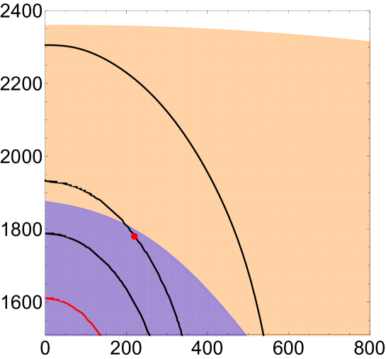
Figure 4.2: The DM abundance, the Higgs boson mass and the muon $g-2$ in $m_{0}-m_{1/2}$ plane. The DM mass is fixed to be 111 GeV ($y(=Y)=2.1$). The Higgs boson with a mass between 122 to 129 GeV is shown in the orange region. The discrepancy of the muon $g-2$ within 2$\sigma$ level is explained in the blue region. The black contours show values of $\Omega_{\chi_{\Phi}}h^{2}=0.08,0.11,0.30$ from left to right. The red line shows ${\rm Br}(\mu\rightarrow e\gamma)=1.0\times 10^{-14}$. The red circle point is the sample point of our model.

In Fig. 4.1, we plot the contours of the Higgs boson mass, the muon $g-2$, the DM abundance and the branching ratio of $\mu\rightarrow e\gamma$ in $m_{\chi_{\Phi}}-m_{1/2}$ plane. We fix $m_{0}$ to be $m_{1/2}/20$ because the small ratio of $m_{0}$ to $m_{1/2}$ is preferred to explain the muon $g-2$ [5]. It is known that such mass spectra can be obtained in gaugino mediation scenarios [50]. The orange region shows the Higgs boson mass in the range from 122 GeV to 129 GeV. The blue region explains the muon $g-2$ anomaly within 2$\sigma$ level. Three black contours show $\Omega_{\chi_{\Phi}}h^{2}=0.01,\ 0.1,\ 1$ from left to right. We find also that our model numerically satisfies experimental upper bounds of both ${\rm Br}(\tau\rightarrow\mu\gamma)$ and ${\rm Br}(\mu\rightarrow e\gamma)$ in all parameter regions of Fig.4.1 and 4.2. For $\mu\rightarrow e\gamma$, a red line shows ${\rm Br}(\mu\rightarrow e\gamma)=1.0\times 10^{-14}$ as a reference value in both Figures. Above the line, the fraction becomes smaller. For $\tau\rightarrow\mu\gamma$, any values of the fraction are not shown because it is too small to reach the current experimental sensitivity. As seen in the figure, there exits the regions where the Higgs boson mass, the muon $g-2$ and the DM abundance can be explained at the same time. It is noted that the DM abundance highly depends on the DM mass. In our model, the DM mass is mostly determined with only ${\cal O}(1)$ parameters, whereas realistic values of the CKM matrix and fermion masses are reproduced. On top of those, the masses of the vector-like generations are determined by the VEV of the DM (singlet) multiplet $\Phi$. In this sense, the presence of the DM supports the existence of three generations in low energy scales.

In Fig. 4.2 we similarly show the Higgs boson mass, the muon $g-2$, the contours of the DM abundance and the branching ratio of $\mu\rightarrow e\gamma$ in $m_{0}-m_{1/2}$ plane. We set the DM mass $m_{\chi_{\Phi}}$ to be $111$ GeV which means that $y=2.1$ in other words. The orange and blue regions are the same as in Fig. 4.1. The black contours shows values of $\Omega_{\chi_{\Phi}}h^{2}=0.08,0.11,0.3$ form left to right. As seen in Fig. 4.2, the Higgs boson mass, the muon $g-2$ and $\Omega_{\chi_{\Phi}}h^{2}=0.11$ can be explained simultaneously where $m_{1/2}$ is lying in the range between 1500 GeV to 1800 GeV and $m_{0}$ is around 300 GeV. The red circle point in Fig. 4.2 is the sample point of our model: $(m_{1/2},m_{0},y)=(1780,250,2.1)$ . We show typical mass spectrum, the Higgs boson mass, the muon $g-2$, the DM abundance and the branching ratio of $\tau\rightarrow\mu\gamma$ and $\mu\rightarrow e\gamma$ in Table 4.1. In Table 4.1, $M_{3}$ is the gluino mass, $m_{\tilde{N}_{1}}$ is the lightest neutralino in the MSSM sector, $m_{\tilde{C}_{1}}$ is the lightest chargino, $m_{\text{stop}}$ is lighter stop mass, $m_{t^{\prime}}$ is the mass of vector-like generations for up-type quark, $m_{\text{charged slepton}}$ is mass of the lightest charged slepton which is the vector-like generations one, $m_{L^{\prime}}$ is the mass of vector-like generations for charged lepton.

	Sample Point (1)
$m_{1/2}$	1780
$m_{0}$	250
$y(=Y)$	2.1
$M_{3}$	1202
$m_{\tilde{N}_{1}}$	347.4
$m_{\tilde{C}_{1}}$	587.5
$m_{\text{stop}}$	1394
$m_{t^{\prime}}$	1157
$m_{\text{charged slepton}}$	324.0
$m_{L^{\prime}}$	274.4
$m_{h^{0}}$	125.2
$\Delta a_{\mu}$	$10.3\times 10^{-10}$
$\Omega_{\chi_{\Phi}}h^{2}$	0.116
${\rm Br}(\tau\rightarrow\mu\gamma)$	$5.5\times 10^{-13}$
${\rm Br}(\mu\rightarrow e\gamma)$	$6.9\times 10^{-15}$

Table 4.1: The sample points in our model. All the mass parameters are given in unit of GeV. $m_{\tilde{N}_{1}}$ is the lightest neutralino in the MSSM sector, $m_{\tilde{C}_{1}}$ is the lightest chargino, $m_{t^{\prime}}$ is the mass of fourth generations for up-type quark, $m_{L^{\prime}}$ is the mass of fourth generations for charged lepton. $\mu_{H}(\sim 2~{}\text{TeV})$ and $b$ terms are determined so that the electroweak symmetry breaking occurs.

Mixings of the vector-like generations with the three generations make a electric dipole moment (EDM). We show typical values of the electron EDM $d_{e}$ and then discuss the constraints from experiments. The contributions are mainly from four sources: the chargino exchange, the neutralino exchange, the $W$ boson exchange and the $Z$ boson exchange. Each contribution is estimated as following [51].

• chargino contribution

  $$|d_{e}^{\chi^{+}}|\sim 8.7\times 10^{-29}e\ {\rm cm}\left(\frac{m_{\tilde{W}}}{600\ {\rm GeV}}\right)\left(\frac{900\ {\rm GeV}}{m_{\tilde{\nu}_{e}}}\right)^{2}\left(\frac{|c_{L\tilde{\nu}_{e}\tilde{W}}c_{R\tilde{\nu}_{e}\tilde{W}}|}{10^{-5}}\right)\left(\frac{{\rm arg}\left(c_{L\tilde{\nu}_{e}\tilde{W}}c_{R\tilde{\nu}_{e}\tilde{W}}\right)}{1.1\times 10^{-4}}\right),$$ (4.16)

  where $m_{\tilde{\nu}_{e}}$ is the mass of snutrino, $m_{\tilde{W}}$ is wino mass, and $c_{L\tilde{\nu_{e}}\tilde{W}}$ and $c_{R\tilde{\nu_{e}}\tilde{W}}$ are couplings of mixings defined in appendix. B.2.

• neutralino contribution

  $$|d_{e}^{\chi^{0}}|\sim 8.7\times 10^{-29}e\ {\rm cm}\left(\frac{m_{\tilde{B}}}{300\ {\rm GeV}}\right)\left(\frac{1000\ {\rm GeV}}{m_{\tilde{e}_{1}}}\right)^{2}\left(\frac{|n_{L\tilde{e}_{1}\tilde{B}}n_{R\tilde{e}_{1}\tilde{B}}|}{10^{-5}}\right)\left(\frac{{\rm arg}\left(n_{L\tilde{e}_{1}\tilde{B}}n_{R\tilde{e}_{1}\tilde{B}}\right)}{2.2\times 10^{-4}}\right),$$ (4.17)

  where $\tilde{e}_{1}$ is the mass of lighter selectron, $m_{\tilde{B}}$ is bino mass, and $n_{L\tilde{e}_{i}\tilde{B}}$ and $c_{R\tilde{e}_{i}\tilde{B}}$ are couplings of mixings.

• W boson contribution

  $$|d_{e}^{W}|\sim 5.9\times 10^{-30}e\ {\rm cm}\left(\frac{m_{L^{\prime}}}{300\ {\rm GeV}}\right)\left(\frac{80\ {\rm GeV}}{m_{W}}\right)^{2}\left(\frac{|g^{WL}_{\nu_{4}e}g^{WR}_{\nu_{4}e}|}{10^{-11}}\right)\left(\frac{{\rm arg}\left(g^{WL}_{\nu_{4}e}g^{WR}_{\nu_{4}e}\right)}{10^{-1}}\right),$$ (4.18)

  where $m_{L^{\prime}}$ is the vector-like lepton mass, and $g^{WL}_{\nu_{4}e}$ and $g^{WR}_{\nu_{4}e}$ are couplings of mixings.

• Z boson contribution

  $$|d_{e}^{Z}|\sim 4.6\times 10^{-30}e\ {\rm cm}\left(\frac{m_{L^{\prime}}}{300\ {\rm GeV}}\right)\left(\frac{90\ {\rm GeV}}{m_{Z}}\right)^{2}\left(\frac{|g^{ZL}_{e_{4}e}g^{ZR}_{e_{4}e}|}{10^{-11}}\right)\left(\frac{{\rm arg}\left(g^{ZL}_{e_{4}e}g^{ZR}_{e_{4}e}\right)}{10^{-1}}\right),$$ (4.19)

  where $g^{ZL}_{\nu_{4}e}$ and $g^{ZR}_{\nu_{4}e}$ are couplings of mixings.

Among of them, the chargino and neutralino exchanges are the main contributions to $d_{e}$. Since the $\mu$ term of our model is around $2~{}{\rm TeV}$, the Higgsinos decouple from the mixing and its couplings are smaller than those of the gauninos. Thus, $d_{e}$ is manly given by the exchange of the gauginos. From experiments, its value is constrained as [52]

$$|d_{e}|<8.7\times 10^{-29}e\ {\rm cm}~{}~{}({\rm EXP}).$$ (4.20)

Therefore, the CP phase of the couplings should satisfy

$$\theta<1.1\times 10^{-4},$$ (4.21)

where $\theta$ represents each phase.

5 Conclusion and Discussion

In this paper we studied the flavor structure in a model with vector-like generations by using Froggatt-Nielsen mechanism. It is notable that the assignment of FN charges can be determined so that the CKM matrix and fermion masses at the $M_{Z}$ scale are reproduced. Furthermore, under such FN charge assignments, the fermion component of the gauge singlet superfield becomes a candidate of DM. The DM mass is induced through the RG flow including the flavor textures which can explain observed flavor physics of muon $g-2$. With such flavor textures, it is found that there exists parameter regions where we can explain the Higgs boson mass, the muon $g-2$ and the DM abundance simultaneously. The singlet plays two roles: One is to fix the vector-like mass by the VEV, and another is that its fermion component is a DM candidate. In this sense, the presence of the DM supports the existence of three generations in low energy scales.

Let us here discuss about the prospect for discovering the DM particle $\chi$ at direct/indirect detection experiments. In our model, the singlino $\chi$ couples to the first generation of the quark field mediated by the scalar component of the vector-like particle. By integrating out the mediator field, we obtain the effective interaction between DM and first generation as ${\cal L}_{\rm int}\simeq(y_{1}^{2}/m^{2})\bar{\chi}\bar{Q}_{1}\chi Q_{1}$. Here $m$ is the mass of the mediator field of order ${\cal O}({\rm TeV})$, and $y_{1}$ is the Yukawa coupling constant. With this interaction, $\chi$ scatters nucleons spin-independently with the cross section $\sigma_{\rm SI}^{N}=y_{1}^{4}\times{\cal O}(10^{2})\,{\rm pb}\,(\mu_{\chi}/10^{2}\,{\rm GeV})^{2}/(m/{\rm TeV})^{4}$ [53], where $\mu_{\chi}$ is the reduced mass defied as $\mu_{\chi}=m_{N}m_{\chi}/(m_{\chi}+m_{N})$ with nuclei mass $m_{N}$. Since the Yukawa coupling of the singlino to the first generation of the quark is set to the small value by the FN mechanism as $y\simeq 10^{-3}(\epsilon/0.33)^{6}$, we see that the magnitude of the spin independent cross section is reduced to $\sigma_{SI}^{N}\simeq 10^{-10}{\rm pb}.$ Thus, in the future direct detection experiments such as XENON1T [54] or DARWIN [55], our DM model will be tested. In the lepton sector, $\chi$ interacts with third generations by larger coupling $y^{2}\simeq 10^{-1}(\epsilon/0.33)^{2}$ mediated by the vector like particle. Thus, through the annihilation of the DM particles in the Galactic Center or in the dwarf spheroidal galaxies, a significant excess of gamma rays might be produced. The excess of the energetic gamma ray might be detected in indirect detection experiments such as Fermi-LAT [56, 57] or CTA [58].

In the present paper, we have studied the thermal production of the DM through the interactions with the quarks and leptons, respecting the original model [5] shown in (2.6), but from the arguments based on symmetries, there can be allowed other terms such as $W\propto\Phi,~{}\Phi^{2}$ or $\Phi H_{u}H_{d}$. In this paper, we have just dropped these terms by hands following [5], but the terms might affect the DM abundance. We will investigate the effects in the future work, but here briefly discuss the issues. Among the interactions, the coupling of the singlet fields with the Higgs fields

$$W=\lambda\Phi H_{u}H_{d}$$ (5.1)

might give a large contributions to the experimental results. This interaction makes the effective $\mu$-term, and contributes to the cross section of the dark matter with nucleons. Thus, to reproduce the result of our analysis and avoid the bound from direct detection experiments, we need to appropriately choose the coupling constants $\lambda$, trilinear coupling $Y$ and the VEV of the singlet field $\braket{\Phi}=V$, but on the other hands it affects muon $g-2$ and Higgs mass corrections. Here we discuss these prospects. With the interaction, the DM components $\chi_{\Phi}$ could have a sizable interaction with nucleons through the t-channel process of the neutral Higgs boson, and it affects the scattering process of the dark matter and nucleons [59, 60]. Especially interactions with the strange-quark mainly contribute to the scattering, and its cross section is given in [60] by

$$\sigma_{\rm SI}^{N}\sim\mu_{\chi}\frac{Y^{2}h_{s}^{2}}{M_{Ha}^{4}}S_{a3}^{2}S_{a1}^{2},$$ (5.2)

where $\mu_{\chi}$ is the reduced mass, $h_{s}$ is Yukawa coupling of the strange quark, $M_{Ha}$ is the Higgs mass, $S_{a3}$ and $S_{a1}$ are diagonalization matrix elements for CP-even neutral Higgs boson (See [60] for the definition), and subscript $a$ runs from $1$ to $3$. The subscript represents the mass eigenstates of the neutral Higgs with order of $M_{H_{1}}<M_{H_{2}}<M_{H_{3}}$. Here the lightest Higgs $H_{1}$ is identified as the detected one of 125 GeV mass [61], and its contribution would be largest. To avoid current bound from the direct detection, we need to choose small value of $Y$, but to reproduce DM mass $m_{\chi_{\Phi}}=YV\simeq 10^{2}{\rm GeV}$, $V$ is required to be larger than $10^{2}{\rm GeV}$. On the other hand, this singlet VEV also gives effective $\mu$-term as $\mu_{\rm eff}=\lambda V$. From the prospect of the Landau pole, $\lambda$ needs to be smaller than unity, and it requires $V$ to be larger than $10^{2}{\rm GeV}$ to satisfy $\mu_{\rm eff}=2{\rm TeV}$. Further, since the scattering of the DM with the SM quarks is mediated through the interaction(5.1), the smaller value of $\lambda$ is also required to avoid the experimental bounds on the spin-independent cross section (5.2). This large value of $V$ leads to the decoupling limit of vector-like generations (i.e., the MSSM-like limit), and then the contributions from the vector-like generations to the Higgs mass and the muon $g-2$ might be too small to explain the experimental values simultaneously. Moreover, the Higgs mass has to be evaluated by taking into account corrections from a coupling $\lambda$. As for the thermal production process, the DM becomes more likely to annihilates into the SM particles mediated by the Higgs fields due to the interaction with the Higgs fields. Thus, we can expect that larger DM mass is required to explain the observed abundance. On the other hand, the interaction might be forbidden by some symmetry such as the R-symmetry. However, at the same time, several terms of the Yukawa interactions (2.9) would be also inevitably absent by the assignment, and the absence would change the muon $g-2$. We investigate these issues in the future work.

Within the FN charge assignment in Table 2.2, flavor violating processes induced by the mixing between $\tau_{R}\leftrightarrow\mu_{R}$ or $d_{R}\leftrightarrow s_{R}$ could be allowed. In this case, the SUSY flavor problem is not avoided by the assignment without a high scale SUSY breaking or a flavor blind mediation mechanism, but there would be other choices such that the off-diagonal elements of squark mass matrix is suppressed and we avoid the problem. In our model, since the mSUGRA scenario is assumed, the Yukawa matrices of the SUSY breaking sector are diagonal. Thus, the SUSY flavor problem is avoided.

We have not taken into account the presence of right-handed neutrino, the relevant flavor textures, and collider physics in this paper. These are important to test our model. We will reveal these prospects in the future work.

Appendix A Annihilation cross section

In this Appendix, we give the expressions of $a$ and $b$ in Eq. (3.15) which are needed to calculate the DM abundance. We calculate $a$ and $b$ in the following way. First, as in Fig. 3.1, we consider the DM annihilation into the SM fermions, which is denoted by $f_{i}$ (except top quark) by exchanging sfermions, which is denoted by $\tilde{f}_{\alpha}$. Next, we evaluate square of the scattering amplitude, which is given by t-channel and u-channel process, as the annihilation cross section $\sigma_{\text{ann}}$. Lastly, we derive the thermal averaged cross section $\left<\sigma_{\text{ann}}v_{\text{rel}}\right>=a+b/x_{F}$ followed by [26]. In the limit where the mass of final state in DM annihilation can be ignored, compared with the DM mass, the coefficients $a$ and $b$ are defined by

$$a = a^{0},$$ (A.1)

$$b = -3a_{0}+b_{0}.$$

After straightforwardly calculations, $a_{0}$ and $b_{0}$ are given by

$$a_{0} = \frac{m_{\chi_{\Phi}}^{2}}{2^{5}\pi}\left[\sum_{\alpha,\beta,i,j}\frac{(O_{Ri\alpha}O_{Rj\beta}+O_{Li\alpha}O_{Lj\beta})^{2}}{\Delta_{\tilde{f}_{\alpha}}\Delta_{\tilde{f}_{\beta}}}-\sum_{\alpha,\beta,i,j}\frac{O_{Ri\alpha}^{2}O_{Rj\beta}^{2}+O_{Li\alpha}^{2}O_{Rj\beta}^{2}}{\Delta_{\tilde{f}_{\alpha}}\Delta_{\tilde{f}_{\beta}}}\right],$$ (A.2)

$$b_{0} = \frac{m_{\chi_{\Phi}}^{2}}{2^{5}\pi}\sum_{\alpha,\beta,i,j}\frac{O_{Ri\alpha}O_{Rj\beta}O_{Li\alpha}O_{Lj\beta}}{\Delta_{\tilde{f}_{\alpha}}^{3}\Delta_{\tilde{f}_{\beta}}^{3}}\times$$

$$\left\{\Delta_{\tilde{f}_{\alpha}}\Delta_{\tilde{f}_{\beta}}\left(2m_{\chi_{\Phi}}^{4}+10m_{\chi_{\Phi}}^{2}m_{\tilde{f}_{\alpha}}^{2}-30m_{\chi_{\Phi}}^{2}m_{\tilde{f}_{\beta}}^{2}-30m_{\tilde{f}_{\alpha}}^{2}m_{\tilde{f}_{\beta}}^{2}\right)+12m_{\chi_{\Phi}}^{8}-2m_{\chi_{\Phi}}^{6}m_{\tilde{f}_{\alpha}}^{2}\right.$$

$$\left.+m_{\chi_{\Phi}}^{6}m_{\tilde{f}_{\beta}}^{2}-16m_{\chi_{\Phi}}^{4}m_{\tilde{f}_{\alpha}}^{4}+m_{\chi_{\Phi}}^{4}m_{\tilde{f}_{\beta}}^{4}-4m_{\chi_{\Phi}}^{4}m_{\tilde{f}_{\alpha}}^{2}m_{\tilde{f}_{\beta}}^{2}-13m_{\chi_{\Phi}}^{2}m_{\tilde{f}_{\alpha}}^{4}m_{\tilde{f}_{\beta}}^{2}+3m_{\chi_{\Phi}}^{2}m_{\tilde{f}_{\alpha}}^{2}m_{\tilde{f}_{\beta}}^{4}\right.$$

$$\left.+2m_{\tilde{f}_{\alpha}}^{4}m_{\tilde{f}_{\beta}}^{4}\right\}$$

$$+\frac{m_{\chi_{\Phi}}^{2}}{2^{5}\pi}\sum_{\alpha,\beta,i,j}\frac{(O_{Ri\alpha}O_{Rj\beta}+O_{Li\alpha}O_{Lj\beta})^{2}}{\Delta_{\tilde{f}_{\alpha}}^{3}\Delta_{\tilde{f}_{\beta}}^{3}}\times$$

$$\left\{-24\Delta_{\tilde{f}_{\alpha}}\Delta_{\tilde{f}_{\beta}}(m_{\chi_{\Phi}}^{4}-m_{\tilde{f}_{\alpha}}^{2}m_{\tilde{f}_{\beta}}^{2})+10m_{\chi_{\Phi}}^{8}+6m_{\chi_{\Phi}}^{6}m_{\tilde{f}_{\alpha}}^{2}+6m_{\chi_{\Phi}}^{6}m_{\tilde{f}_{\beta}}^{2}-26m_{\chi_{\Phi}}^{4}m_{\tilde{f}_{\alpha}}^{2}m_{\tilde{f}_{\beta}}^{2}\right.$$

$$\left.+4m_{\chi_{\Phi}}^{4}m_{\tilde{f}_{\alpha}}^{4}+4m_{\chi_{\Phi}}^{4}m_{\tilde{f}_{\beta}}^{4}-8m_{\chi_{\Phi}}^{2}m_{\tilde{f}_{\alpha}}^{4}m_{\tilde{f}_{\beta}}^{2}-8m_{\chi_{\Phi}}^{2}m_{\tilde{f}_{\alpha}}^{2}m_{\tilde{f}_{\beta}}^{4}\right\}$$

$$+\frac{m_{\chi_{\Phi}}^{2}}{2^{5}\pi}\sum_{\alpha,\beta,i,j}\frac{(O_{Ri\alpha}^{2}O_{Rj\beta}^{2}+O_{Li\alpha}^{2}O_{Lj\beta}^{2})}{\Delta_{\tilde{f}_{\alpha}}^{3}\Delta_{\tilde{f}_{\beta}}^{3}}\times$$

$$\left\{\Delta_{\tilde{f}_{\alpha}}\Delta_{\tilde{f}_{\beta}}(3m_{\chi_{\Phi}}^{4}+2m_{\chi_{\Phi}}^{2}m_{\tilde{f}_{\alpha}}^{2}+m_{\chi_{\Phi}}^{2}m_{\tilde{f}_{\beta}}^{2}-2m_{\tilde{f}_{\alpha}}^{2}m_{\tilde{f}_{\beta}}^{2})-16m_{\chi_{\Phi}}^{8}-16m_{\chi_{\Phi}}^{6}m_{\tilde{f}_{\alpha}}^{2}\right.$$

$$\left.-16m_{\chi_{\Phi}}^{6}m_{\tilde{f}_{\beta}}^{2}-8m_{\chi_{\Phi}}^{4}m_{\tilde{f}_{\alpha}}^{4}-8m_{\chi_{\Phi}}^{4}m_{\tilde{f}_{\beta}}^{4}\right\},$$

where $\Delta_{\tilde{f}_{\alpha,\beta}}\equiv m_{\chi_{\Phi}}^{2}+m_{\tilde{f}_{\alpha,\beta}}^{2}$, the subscript $i,j$ correspond to the generation of the SM particles whose the mass is below the freeze-out temperature and the subscript $\alpha,\beta$ corresponds to the generations of sfermions which is regarded as the mediator between the DM and the SM particles in our model. The dependence of $a$ and $b$ on the DM and sfermion masses is roughly given by

$$a,b\sim\frac{O^{4}}{m_{\tilde{f}}^{2}}\frac{m_{\chi_{\Phi}}^{2}}{m_{\tilde{f}}^{2}}\sim\frac{y^{4}}{m_{\tilde{f}}^{2}}\frac{m_{\chi_{\Phi}}^{2}}{m_{\tilde{f}}^{2}},$$ (A.4)

where $O$ means the coupling constants between the DM and sfermions and $y$ is a Yukawa coupling between them.

Appendix B Analytic formulae for Higgs mass and muon $g-2$

B.1 Higgs mass

The one-loop correction to the lightest neutral Higgs mass $\Delta m^{2}_{h}$ is given by [30]

$$\Delta m_{h}^{2} =\Bigg{[}\dfrac{\sin^{2}\beta}{2}\left(\dfrac{\partial^{2}}{\partial v_{u}^{2}}-\dfrac{1}{v_{u}}\dfrac{\partial}{\partial v_{u}}\right)+\dfrac{\cos^{2}\beta}{2}\left(\dfrac{\partial^{2}}{\partial v_{d}^{2}}-\dfrac{1}{v_{d}}\dfrac{\partial}{\partial v_{d}}\right)$$ (B.1)

$$\qquad+\sin\beta\cos\beta\dfrac{\partial^{2}}{\partial v_{u}\partial v_{d}}\Bigg{]}\Delta V_{H}$$

where $\Delta V_{H}$ is the one-loop corrections to the Higgs potential and is defined as

$$\qquad\Delta V_{H}=\sum_{X=u,d,e}\,\sum_{i=1}^{10}2N_{c}\left[F(m_{\tilde{X}_{i}}^{2})-F(m_{X_{i}}^{2})\right],\hskip 19.91692ptN_{c}=\begin{cases}3&(X=u,d)\\ 1&(X=e)\end{cases}$$ (B.2)

where $m_{X_{i}}^{2}$ and $m_{\tilde{X}_{i}}^{2}$ are the squared-mass eigenvalues of fermions and scalars, respectively, which are obtained by diagonalizing (2.13)-(2.15) for fermions ($M_{u}^{\dagger}M_{u}$ and $M_{u}M_{u}^{\dagger}$, etc.). For diagonalization of scalars mass matrices, we use the scalar mass matrices which are defined in Eq. (B.1)–(B.3) in [5]. The function $F$ is defined as [30]

$$F(x)=\frac{x^{2}}{64\pi^{2}}\left[\ln\left(\frac{x}{\mu^{2}}\right)-\frac{3}{2}\right],$$ (B.3)

where $\mu$ represents the renormalization scale which is set to be $M_{\text{SUSY}}$ in evaluating the Higgs mass.

B.2 Muon g-2

We show the SUSY contributions $\Delta a_{\mu}^{\rm SUSY}$ and non-SUSY contributions $\Delta a_{\mu}^{\rm non-SUSY}$ in Eq. (4.2). First, we consider the SUSY contributions. In order to calculate the SUSY contributions, we use the mass eigenstate basis for gauginos, charged leptons, charged sleptons and neutral sleptons. The analytic formula of SUSY contributions is the same as the previous paper [5]. Let us define the diagonalization matrix for neutralinos, charginos, sneutrinos, in order to evaluate the SUSY contributions $\Delta a_{\mu}^{\rm SUSY}$ of the muon $g-2$. In the basis of {$\tilde{B},\tilde{W}^{0},\tilde{H}^{0}_{d},\tilde{H}^{0}_{u}$}, the neutralino mass matrix $M_{\chi^{0}}$ is given by

$$M_{\chi^{0}}=\left(\begin{array}[]{cccc}M_{1}&0&-g_{1}v_{d}/\sqrt{2}&g_{1}v_{u}/\sqrt{2}\\ 0&M_{2}&g_{2}v_{d}/\sqrt{2}&-g_{2}v_{u}/\sqrt{2}\\ -g_{1}v_{d}/\sqrt{2}&g_{2}v_{d}/\sqrt{2}&0&-\mu_{H}\\ g_{1}v_{u}/\sqrt{2}&-g_{2}v_{u}/\sqrt{2}&-\mu_{H}&0\end{array}\right).$$ (B.8)

In the basis of {$\tilde{W}^{-},\tilde{H}_{d}^{-}$} and {$\tilde{W}^{+},\tilde{H}_{u}^{+}$}, the chargino mass matrix $M_{\chi^{\pm}}$ is given by

$$M_{\chi^{\pm}}=\left(\begin{array}[]{cc}M_{2}&\sqrt{2}gv_{u}\\ \sqrt{2}gv_{d}&\mu_{H}\end{array}\right),$$ (B.11)

where the charged wino $\tilde{W}^{\pm}$ are defined as

$$\tilde{W}^{\pm}=\frac{i}{\sqrt{2}}(\tilde{W}^{1}\mp i\tilde{W}^{2}).$$ (B.12)

By using the neutralino mixing matrix $N$ and the chargino mixing matrices $J,K$, the mass matrix in Eq. (B.8) and (B.11) are diagonalized by

$$NM_{\chi^{0}}N^{\dagger} ={\rm diag}\big{(}\,m_{\chi^{0}_{1}},m_{\chi^{0}_{2}},m_{\chi^{0}_{3}},m_{\chi^{0}_{4}}\big{)},$$ (B.13)

$$JM_{\chi^{\pm}}K^{\dagger} ={\rm diag}\big{(}m_{\chi^{\pm}_{1}},m_{\chi^{\pm}_{2}}\big{)},$$ (B.14)

where $m_{\chi^{0}_{x}}$ ($x=1,\ldots,4$) are the positive mass eigenvalues ($m_{\chi^{0}_{x}}<m_{\chi^{0}_{y}}$, if $x<y$), and $m_{\chi_{x}}^{\pm}$ ($x=1,2$) are the positive mass eigenvalues ($m_{\chi^{\pm}_{1}}<m_{\chi^{\pm}_{2}}$). The diagonalization of neutral sleptons are defined by

$$(U_{\tilde{\nu}}M^{2}_{\tilde{\nu}}U_{\tilde{\nu}}^{\dagger})_{\alpha\beta} =m^{2}_{\tilde{N}_{\alpha}}\delta_{\alpha\beta}\hskip 14.22636pt(\alpha,\beta=1,\dots,5),$$ (B.15)

where $M_{\nu}^{2}$ is the neutral slepton mass matrix defined in [5].

The SUSY contributions to the muon $g-2$ are divided into three parts: neutralinos ($\chi^{0}$), charginos ($\chi^{\pm}$) and singlino ($\chi_{\Phi}$). The singlino contribution is calculated by the replacement of $\chi^{0}$ with $\chi_{\Phi}$ in the neutralino diagram (with appropriate replacement of coefficients). The SUSY contributions are given by

$$\Delta a_{\mu}^{\rm SUSY}=\Delta a_{\mu}^{\chi^{0}}+\Delta a_{\mu}^{\chi^{\pm}}+\Delta a_{\mu}^{\chi_{\Phi}},$$ (B.16)

where

$$\Delta a_{\mu}^{\chi^{0}} =\sum_{a,x}\frac{1}{16\pi^{2}}\bigg{[}\frac{m_{\mu}m_{\chi^{0}_{x}}}{m^{2}_{\tilde{E}_{a}}}n_{2ax}^{L}n_{2ax}^{R}F_{2}^{N}(r_{1ax})-\frac{m_{\mu}^{2}}{6m^{2}_{\tilde{E}_{a}}}\big{(}n_{2ax}^{L}n_{2ax}^{L}+n_{2ax}^{R}n_{2ax}^{R}\big{)}F_{1}^{N}(r_{1ax})\bigg{]},$$ (B.17)

$$\Delta a_{\mu}^{\chi^{\pm}} =\sum_{\alpha,x}\frac{1}{16\pi^{2}}\bigg{[}\frac{-3m_{\mu}m_{\chi_{x}}^{\pm}}{m^{2}_{\tilde{\nu}_{a}}}c_{2\alpha x}^{L}c_{2\alpha x}^{R}F_{2}^{C}(r_{2\alpha x})+\frac{m_{\mu}^{2}}{3m^{2}_{\tilde{\nu}_{\alpha}}}\big{(}c_{2\alpha x}^{L}c_{2\alpha x}^{L}+c_{2\alpha x}^{R}c_{2\alpha x}^{R}\big{)}F_{1}^{C}(r_{2\alpha x})\bigg{]},$$ (B.18)

$$\Delta a_{\mu}^{\chi_{\Phi}} =\sum_{a}\frac{1}{16\pi^{2}}\bigg{[}\frac{m_{\mu}m_{\chi_{\Phi}}}{m^{2}_{\tilde{E}_{a}}}s_{a}^{L}s_{a}^{R}F_{2}^{N}(r_{3a})-\frac{m_{\mu}^{2}}{6m^{2}_{\tilde{E}_{a}}}\big{(}s_{2a}^{L}s_{2a}^{L}+s_{2a}^{R}s_{2a}^{R}\big{)}F_{1}^{N}(r_{3a})\bigg{]},$$ (B.19)

with $r_{1ax}=m^{2}_{\chi^{0}_{x}}/m^{2}_{\tilde{E}_{a}}$, $r_{2\alpha x}=m^{2}_{\chi^{\pm}_{x}}/m^{2}_{\tilde{N}_{\alpha}}$, $r_{3a}=m^{2}_{\chi_{\Phi}}/m^{2}_{\tilde{E}_{a}}$, and $m_{\mu}$ is the muon mass, the function $F_{1,2}^{N}$ and $F_{1,2}^{C}$ are defined by

$$F_{1}^{N}(x)=\frac{2}{(1-x)^{4}}\left(1-6x^{2}+3x^{3}+2x^{3}-6x^{2}\ln x\right),$$ (B.20)

$$F_{2}^{N}(x)=\frac{3}{(1-x)^{3}}\left(1-x^{2}+2x\ln x\right),$$ (B.21)

$$F_{1}^{C}(x)=\frac{2}{(1-x)^{4}}\left(2+3x-6x^{2}+x^{3}+6x\ln x\right),$$ (B.22)

$$F_{2}^{C}(x)=\frac{-3}{(1-x)^{3}}\left(3-4x+x^{2}+2\ln x\right),$$ (B.23)

and by using diagonalization matrices Eq. (3.5), (3.8), (B.13), (B.14) and (B.15), the coefficients $n_{Iax}^{L,R},c_{I\alpha x}^{L,R},s_{Ia}^{L,R}$ in Eq. (B.17)–(B.19) are defined by

$$n^{L}_{Iax} =-\sum_{i,j=1}^{4}(y_{e})_{ij}(V_{e_{R}})_{iI}(U_{\tilde{e}})_{aj}N_{x3}+y_{\bar{e}}(V_{e_{R}})_{5I}(U_{\tilde{e}})_{a,10}N_{x4}$$

$$\qquad-\sum_{i=1}^{4}\sqrt{2}g_{1}(V_{e_{R}})_{iI}(U_{\tilde{e}})_{a,i+5}N_{x1}-\frac{g_{2}}{\sqrt{2}}(V_{e_{R}})_{5I}(U_{\tilde{e}})_{a5}N_{x2}$$

$$\qquad-\frac{g_{1}}{\sqrt{2}}(V_{e_{R}})_{5I}(U_{\tilde{e}})_{a5}N_{x1},$$ (B.24)

$$n^{R}_{Iax} =\sum_{i,j=1}^{4}(y_{e})_{ij}(V_{e_{L}})_{jI}(U_{\tilde{e}})_{a,i+5}N_{x3}-y_{\bar{e}}(V_{e_{L}})_{5I}(U_{\tilde{e}})_{a5}N_{x4}$$

$$\qquad+\sum_{i=1}^{4}\bigg{[}\frac{g_{2}}{\sqrt{2}}(V_{e_{L}})_{iI}(U_{\tilde{e}})_{ai}N_{x2}+\frac{g_{1}}{\sqrt{2}}(V_{e_{L}})_{iI}(U_{\tilde{e}})_{ai}N_{x1}\bigg{]}$$

$$\qquad+\sqrt{2}g_{1}(V_{e_{L}})_{5I}(U_{\tilde{e}})_{a,10}N_{x1},$$ (B.25)

$$c^{L}_{Iax} =-\sum_{i,j=1}^{4}(y_{e})_{ij}(V_{e_{R}})_{iI}(U_{\tilde{\nu}})_{aj}J_{x2}+g_{2}(V_{e_{R}})_{5I}(U_{\tilde{\nu}})_{a5}J_{x1},$$ (B.26)

$$c^{R}_{Iax} =y_{\bar{e}}(V_{e_{L}})_{5I}(U_{\tilde{\nu}})_{a5}K_{x2}-\sum_{i=1}^{4}g_{2}(V_{e_{L}})_{iI}(U_{\tilde{\nu}})_{ai}K_{x1},$$ (B.27)

$$s_{Ia}^{L} =\sum_{i=1}^{4}\Big{[}-{y_{e}}_{i}(V_{e_{R}})_{iI}(U_{\tilde{e}})_{a,10}-{y_{L}}_{i}(V_{e_{R}})_{5I}(U_{\tilde{e}})_{ai}\Big{]},$$ (B.28)

$$s^{R}_{Ia} =\sum_{i=1}^{4}\Big{[}-{y_{e}}_{i}(V_{e_{L}})_{5I}(U_{\tilde{e}})_{a,i+5}-{y_{L}}_{i}(V_{e_{L}})_{iI}(U_{\tilde{e}})_{a5}\Big{]}.$$ (B.29)

Next, we show the non-SUSY contributions. The contributions from vector-like fermions to the muon $g-2$ are investigated in detail in [32] and we derive $\Delta a_{\mu}^{\rm non-SUSY}$ in accordance with [32]. We use the mass eigenstate basis for charged leptons, neutral leptons and CP-even neutral Higgs bosons. Let us define the diagonalization matrix for neutral leptons and CP-even Higgs boson in order to evaluate the non-SUSY contributions of the muon $g-2$ ($\Delta a_{\mu}^{\rm non-SUSY}$). Neutral lepton mass matrix $M_{\nu}$ can be read in the superpotential (2.9) and is given by

$$M_{\nu} = \bordermatrix{&\nu_{1R}&\nu_{2R}&\nu_{3R}&\nu_{4R}&\nu_{5R}\cr\nu_{1L}&&&&&Y_{L_{1}}\epsilon^{4}V\cr\nu_{2L}&&&&&Y_{L_{2}}\epsilon^{3}V\cr\nu_{3L}&&&&&Y_{L_{3}}\epsilon^{2}V\cr\nu_{4L}&&&&&Y_{L_{4}}\epsilon^{1}V\cr\nu_{5L}&&&&&\cr},$$ (B.30)

where blank elements mean zero. The diagonalization of this matrix is defined by

$$(V_{\nu_{R}}M_{\nu}V^{\dagger}_{\nu_{L}})_{ij}=m_{\nu_{i}}\delta_{ij},\hskip 8.53581pt(i,j=1,\cdots,5)$$ (B.31)

where only $m_{\nu_{5}}$ is finite value and other masses ($i=1,\cdots,4$) are zero. The CP-even neutral Higgs mass matrix $M_{h^{0}}^{2}$ is given by

$$M_{h^{0}}^{2}=\left(\begin{array}[]{cc}M_{A}^{2}\sin^{2}\beta+M_{Z}^{2}\cos^{2}\beta&-\left(M_{A}^{2}+M_{Z}^{2}\right)\sin\beta\cos\beta\\ -\left(M_{A}^{2}+M_{Z}^{2}\right)\sin\beta\cos\beta&M_{A}^{2}\cos^{2}\beta+M_{Z}^{2}\sin^{2}\beta\end{array}\right),$$ (B.32)

where $M_{A}=2b/\sin(2\beta)$ is the CP-odd neutral Higgs boson mass as in the MSSM. This diagonalization of this matrix is defined by

$$(U_{h^{0}}M_{h^{0}}^{2}U^{\dagger}_{h^{0}})_{XY}=m^{2}_{h^{0}_{X}}\delta_{XY},\hskip 8.53581pt(X,Y=1,2)$$ (B.33)

where the mass eigenvalues are ordered as $m_{h^{0}_{1}}<m_{h^{0}_{2}}$.

The non-SUSY contributions are divided into 3 parts: $W$-boson, $Z$-boson and Higgs bosons. Then, $\Delta a_{\mu}^{\rm non-SUSY}$ is given by

$$\Delta a_{\mu}^{\rm non-SUSY}=\Delta a_{\mu}^{Z}+\Delta a_{\mu}^{W}+\Delta a_{\mu}^{h},$$ (B.34)

where

$$\Delta a_{\mu}^{Z} =-\frac{m_{\mu}}{8\pi^{2}M_{Z}^{2}}\sum_{a=4,5}\left[\left((g_{2a}^{ZL})^{2}+(g^{ZR}_{2a})^{2}\right)m_{\mu}F_{Z}(x_{Za})+g_{2a}^{ZL}g_{2a}^{ZR}m_{E_{a}}G_{Z}(x_{Za})\right],$$ (B.35)

$$\Delta a_{\mu}^{W} =-\frac{m_{\mu}}{16\pi^{2}M_{W}^{2}}\left[\left((g^{WL}_{52})^{2}+(g^{WR}_{52})^{2}\right)m_{\mu}F_{W}(x_{W})+g^{WL}_{52}g^{WR}_{52}m_{\nu_{5}}G_{W}(x_{W})\right],$$ (B.36)

$$\Delta a_{\mu}^{h} =-\sum_{X=1,2}\sum_{a=4,5}\frac{m_{\mu}}{32\pi^{2}m_{h^{0}_{X}}^{2}}\left[\left((\lambda_{2aX})^{2}+(\lambda_{a2X})^{2}\right)m_{\mu}F_{h}(x_{h^{0}aX})+\lambda_{2aX}\lambda_{a2X}m_{E_{a}}G_{h}(x_{h^{0}aX})\right],$$ (B.37)

with $x_{Za}=m_{E_{a}}^{2}/M_{Z}^{2}$, $x_{W}=m_{\nu_{5}}^{2}/M_{W}^{2}$, $x_{h^{0}aX}=m_{E_{a}}^{2}/m_{h^{0}_{X}}^{2}$, and $M_{W}$ is the $W$-boson mass, $m_{E_{a}}$ is the mass eigenvalues of charged lepton defined in Eq. (3.5), the function $F_{Z},F_{W},F_{h},G_{Z},G_{W},G_{h}$ are defined by [32]

$$F_{Z}(x)=\frac{12}{(1-x)^{4}}\left(8-38x+39x^{2}-14x^{3}+5x^{4}-18x^{2}\ln x\right),$$ (B.38)

$$F_{W}(x)=\frac{-6}{(1-x)^{4}}\left(10-43x+78x^{2}-49x^{3}+4x^{4}+18x^{3}\ln x\right),$$ (B.39)

$$F_{h}(x)=\frac{12}{(1-x)^{4}}\left(8-38x+39x^{2}-14x^{3}+5x^{4}-18x^{2}\ln x\right),$$ (B.40)

$$G_{Z}(x)=\frac{2}{(1-x)^{3}}\left(-4+3x+x^{3}-6x\ln x\right),$$ (B.41)

$$G_{W}(x)=\frac{-1}{(1-x)^{3}}\left(-4+15x-12x^{2}+x^{3}+6x^{2}\ln x\right),$$ (B.42)

$$G_{h}(x)=\frac{1}{(1-x)^{3}}\left(3-4x+x^{2}+2\ln x\right).$$ (B.43)

and by using mixing matrices Eq.  (3.5), (B.31) and (B.33), the coefficients $g^{ZL,ZR}_{2a},g^{WL,WR}_{52},\lambda_{2a},\lambda_{a2}$ are defined by

$$g^{ZL}_{xy} =\sum_{i=1}^{4}\frac{g_{2}}{\cos\theta_{W}}\left(-\frac{1}{2}+\sin^{2}\theta_{W}(V_{e_{L}})_{xi}(V_{e_{L}})_{yi}\right)+\frac{g_{2}}{\cos\theta_{W}}\sin^{2}\theta_{W}(V_{e_{L}})_{x5}(V_{e_{L}})_{y5},$$ (B.44)

$$g^{ZR}_{xy} =\sum_{i=1}^{4}\frac{-g_{2}}{\cos\theta_{W}}\sin^{2}\theta_{W}(V_{e_{R}})_{xi}(V_{e_{R}})_{yi}+\frac{g_{2}}{\cos\theta_{W}}\left(-\frac{1}{2}+\sin^{2}\theta_{W}\right)(V_{e_{R}})_{x5}(V_{e_{R}})_{y5},$$ (B.45)

$$g^{WL}_{xy} =\sum_{i=1}^{4}\frac{g_{2}}{\sqrt{2}}(V_{\nu_{L}})_{xi}(V_{e_{L}})_{yi},$$ (B.46)

$$g^{WR}_{xy} =\frac{g_{2}}{\sqrt{2}}(V_{\nu_{L}})_{x5}(V_{e_{L}})_{y5},$$ (B.47)

$$\lambda_{xyX} =\sum_{i,j=1}^{4}(V_{e_{R}})_{xi}(y_{e})_{ij}(V_{e_{L}})_{yj}(U_{h^{0}})_{X1}+y_{\bar{e}}(V_{e_{R}})_{x5}(V_{e_{L}})_{y5}(U_{h^{0}})_{X2}$$ (B.48)

where $\theta_{W}$ is the Weinberg angle.

Appendix C Form factors for lepton flavor violation

Following [48, 49], we summarize the form factors which are necessary to evaluate the branching ratio of lepton flavor violating processes as shown in (4.14) and (4.15). The form factors are divided into four parts: neutralinos, charginos, Z-boson and W-boson parts as

$$F_{2}^{\l_{i}l_{j}}(0) =F_{2\chi^{0}}^{l_{i}l_{j}}+F_{2\chi^{+}}^{l_{i}l_{j}}+F_{2Z}^{l_{i}l_{j}}+F_{2W}^{l_{i}l_{j}},$$ (C.1)

$$F_{3}^{\l_{i}l_{j}}(0) =F_{3\chi^{0}}^{l_{i}l_{j}}+F_{3\chi^{+}}^{l_{i}l_{j}}+F_{3Z}^{l_{i}l_{j}}+F_{3W}^{l_{i}l_{j}}.$$ (C.2)

The neutralino contributions are given by

$$F^{l_{i}l_{j}}_{2\chi^{0}} =\sum_{a=1}^{10}\sum_{x=1}^{4}\bigg{[}\frac{-m_{l_{i}}(m_{l_{i}}+m_{l_{j}})}{192\pi^{2}m^{2}_{\chi_{x}^{0}}}\{n^{L}_{iax}n^{L}_{jax}+n^{R}_{iax}n^{R}_{jax}\}F_{1}\left(\frac{M^{2}_{\tilde{E}_{a}}}{m^{2}_{\chi_{x}^{0}}}\right)$$

$$\hskip 51.21495pt-\frac{(m_{l_{i}}+m_{l_{j}})}{64\pi^{2}m_{\chi_{x}^{0}}}\{n^{L}_{iax}n^{R}_{jax}+n^{R}_{iax}n^{L}_{jax}\}F_{2}\left(\frac{M^{2}_{\tilde{E}_{a}}}{m^{2}_{\chi_{x}^{0}}}\right)\bigg{]}\,,$$ (C.3)

$$F^{l_{i}l_{j}}_{3\chi^{0}} =\sum_{a=1}^{10}\sum_{x=1}^{4}\frac{(m_{l_{i}}+m_{l_{j}})m_{\chi_{x}^{0}}}{32\pi^{2}M^{2}_{\tilde{E}_{a}}}\{n^{L}_{iax}n^{R}_{jax}-n^{R}_{iax}n^{L}_{jax}\}F_{3}\left(\frac{m^{2}_{\chi_{x}^{0}}}{M^{2}_{\tilde{E}_{a}}}\right)\,,$$ (C.4)

where the functions are defined by

$$F_{1}(x) =\frac{1}{(x-1)^{4}}\{-x^{3}+6x^{2}-3x-2-6x\ln x\},$$ (C.5)

$$F_{2}(x) =\frac{1}{(x-1)^{3}}\{-x^{2}+1+2x\ln x\},\,$$ (C.6)

$$F_{3}(x) =\frac{1}{2(x-1)^{2}}\{x+1+\frac{2x\ln x}{1-x}\},\,$$ (C.7)

and $n_{iax}^{L,R}$ are given in Eq. (B.24) and (B.2).

The chargino contributions are given by

$$F^{l_{i}l_{j}}_{2\chi^{+}} =\sum_{\alpha=1}^{5}\sum_{x=1}^{2}\bigg{[}\frac{m_{l_{i}}(m_{l_{i}}+m_{l_{j}})}{64\pi^{2}m^{2}_{\chi_{x}^{+}}}\{c^{L}_{i\alpha x}c^{L}_{j\alpha x}+c^{R}_{i\alpha x}c^{R}_{j\alpha x}\}F_{4}\left(\frac{M^{2}_{\tilde{N}_{\alpha}}}{m^{2}_{\chi_{x}^{+}}}\right)$$

$$\hskip 51.21495pt+\frac{(m_{l_{i}}+m_{l_{j}})}{64\pi^{2}m_{\chi_{x}^{+}}}\{c^{L}_{i\alpha x}c^{R}_{j\alpha x}+c^{R}_{i\alpha x}c^{L}_{j\alpha x}\}F_{5}\left(\frac{M^{2}_{\tilde{N}_{\alpha}}}{m^{2}_{\chi_{x}^{+}}}\right)\bigg{]}\,,$$ (C.8)

$$F^{l_{i}l_{j}}_{3\chi^{+}} =\sum_{\alpha=1}^{5}\sum_{x=1}^{2}\frac{(m_{l_{i}}+m_{l_{j}})m_{\chi_{x}^{+}}}{32\pi^{2}M^{2}_{\tilde{N}_{\alpha}}}\{c^{L}_{i\alpha x}c^{R}_{j\alpha x}-c^{R}_{i\alpha x}c^{L}_{j\alpha x}\}F_{6}\left(\frac{m^{2}_{\chi_{x}^{+}}}{M^{2}_{\tilde{N}_{\alpha}}}\right)\,,$$ (C.9)

where the functions are defined by

$$F_{4}(x) =\frac{1}{3(x-1)^{4}}\{-2x^{3}-3x^{2}+6x-1+6x^{2}\ln x\},$$ (C.10)

$$F_{5}(x) =\frac{1}{(x-1)^{3}}\{3x^{2}-4x+1-2x^{2}\ln x\},\,$$ (C.11)

$$F_{6}(x) =\frac{1}{2(x-1)^{2}}\{-x+3+\frac{2\ln x}{1-x}\},\,$$ (C.12)

and $c_{i\alpha x}^{L,R}$ are given in Eq. (B.26) and (B.27).

The contributions from the Z-boson exchange are given by

$$F^{l_{i}l_{j}}_{2Z} =\sum_{a=1}^{5}\frac{{m_{l_{i}}(m_{l_{i}}+m_{l_{j}})}}{64\pi^{2}m^{2}_{Z}}\{g^{ZL}_{ia}g^{ZL}_{ja}+g^{ZR}_{ia}g^{ZR}_{ja}\}F_{Z}\left(\frac{m^{2}_{E_{a}}}{m^{2}_{Z}}\right)$$

$$\hskip 28.45274pt+\frac{{m_{E_{a}}(m_{l_{i}}+m_{l_{j}})}}{64\pi^{2}m^{2}_{Z}}\{g^{ZL}_{ia}g^{ZR}_{ja}+g^{ZR}_{ia}g^{ZL}_{ja}\}G_{Z}\left(\frac{m^{2}_{E_{a}}}{m^{2}_{Z}}\right),$$ (C.13)

$$F^{l_{i}l_{j}}_{3Z} =\sum_{a=1}^{5}\frac{{(m_{l_{i}}+m_{l_{j}})}}{32\pi^{2}}\frac{m_{E_{a}}}{m^{2}_{Z}}\{g^{ZL}_{ia}g^{ZR}_{ja}-g^{ZR}_{ia}g^{ZL}_{ja}\}I_{1}\left(\frac{m^{2}_{E_{a}}}{m^{2}_{Z}}\right)\,,$$ (C.14)

where the functions are defined by

$$F_{Z}(x) =\frac{1}{3(x-1)^{4}}\left[-5x^{4}+14x^{3}-39x^{2}+18x^{2}\ln x+38x-8\right],$$ (C.15)

$$G_{Z}(x) =\frac{2}{(x-1)^{3}}\left[x^{3}+3x-6x\ln x-4\right],$$ (C.16)

$$I_{1}(x) =\frac{2}{(1-x)^{2}}\left[1+\frac{1}{4}x+\frac{1}{4}x^{2}+\frac{3x\ln x}{2(1-x)}\right],\,$$ (C.17)

and $g_{xy}^{ZL,ZR}$ are given in Eq. (B.44) and (B.45).

The contributions from the W-boson exchange are given by

$$F^{l_{i}l_{j}}_{2W} =\frac{{m_{l_{i}}(m_{l_{i}}+m_{l_{j}})}}{32\pi^{2}m^{2}_{W}}\{g^{WL}_{5i}g^{WL}_{5j}+g^{WR}_{5i}g^{WR}_{5j}\}F_{W}\left(\frac{m^{2}_{\nu_{5}}}{m^{2}_{W}}\right)$$

$$\hskip 28.45274pt+\frac{{m_{\nu_{5}}(m_{l_{i}}+m_{l_{j}})}}{32\pi^{2}m^{2}_{W}}\{g^{WL}_{5i}g^{WR}_{5j}+g^{WR}_{5i}g^{WL}_{5j}\}G_{W}\left(\frac{m^{2}_{\nu_{5}}}{m^{2}_{W}}\right),$$ (C.18)

$$F^{l_{i}l_{j}}_{3W} =-\frac{{m_{\nu_{5}}(m_{l_{i}}+m_{l_{j}})}}{32\pi^{2}m^{2}_{W}}\{g^{WL}_{5i}g^{WR}_{5j}-g^{WR}_{5i}g^{WL}_{5j}\}I_{2}\left(\frac{m^{2}_{\nu_{5}}}{m^{2}_{W}}\right)\,,$$ (C.19)

where the functions are defined by

$$F_{W}(x) =\frac{1}{6(x-1)^{4}}\left[4x^{4}-49x^{3}+18x^{3}\ln x+78x^{2}-43x+10\right],$$ (C.20)

$$G_{W}(x) =\frac{1}{(x-1)^{3}}\left[4-15x+12x^{2}-x^{3}-6x^{2}\ln x\right],\,$$ (C.21)

$$I_{2}(x) =\frac{2}{(1-x)^{2}}\left[1-\frac{11}{4}x+\frac{1}{4}x^{2}-\frac{3x^{2}\ln x}{2(1-x)}\right]\,,$$ (C.22)

and $g_{xy}^{WL,WR}$ are given in Eq. (B.46) and (B.47).

Appendix D RG Equations

We present the RG equations of model parameters in our model. Due to the asymptotically non-free nature of the gauge sector, the two-loop RG equations are used for gauge coupling constants and gaugino masses.

D.1 Gauge couplings and gaugino masses

The two-loop RG equations of gauge coupling constants $g_{i}$ and gaugino masses $M_{i}$ ($i=1,2,3$) are given by

$$\frac{dg_{i}}{d(\log\mu)} =b_{i}\frac{g_{i}^{3}}{16\pi^{2}}+\frac{g_{i}^{3}}{(16\pi^{2})^{2}}\bigg{[}\sum_{j}b_{ij}g_{j}^{2}-\sum_{a=u,d,e}c_{ia}\Big{[}{\rm Tr}\big{(}{\bm{y}}_{a}^{\dagger}{\bm{y}}_{a}\big{)}+y_{\bar{a}}^{*}y_{\bar{a}}\Big{]}$$

$$\hskip 156.49014pt-\sum_{k=1}^{4}\sum_{x=Q,u,d,L,e}\!d_{ix}y_{x_{k}}^{*}y_{x_{k}}\bigg{]},$$ (D.1)

$$\frac{dM_{i}}{d(\log\mu)} =2b_{i}\frac{g_{i}^{2}M_{i}}{16\pi^{2}}+\frac{2g_{i}^{2}}{(16\pi^{2})^{2}}\bigg{[}\sum_{j}b_{ij}g_{j}^{2}(M_{i}+M_{j})+\sum_{a=u,d,e}c_{ia}\Big{[}{\rm Tr}\big{(}{\bm{y}}_{a}^{\dagger}{\bm{a}}_{a}\big{)}+y_{\bar{a}}^{*}a_{\bar{a}}$$

$$\qquad-M_{i}\big{[}{\rm Tr}({\bm{y}}_{a}^{\dagger}{\bm{y}}_{a})+y_{\bar{a}}^{*}y_{\bar{a}}\big{]}\Big{]}+\sum_{k=1}^{4}\sum_{x=Q,u,d,L,e}\!\!d_{ix}(y_{x_{k}}^{*}A_{x_{k}}-M_{i}y_{x_{k}}^{*}y_{x_{k}})\bigg{]},$$ (D.2)

where the one-loop beta function coefficients are $b_{i}=(53/5,5,1)$, and the coefficient matrices $b_{ij}$, $c_{ia}$, $d_{ix}$ are

$$b_{ij}=\left(\begin{array}[]{ccc}977/75&39/5&88/3\\ 13/5&53&40\\ 11/3&15&178/3\\ \end{array}\right),$$ (D.6)

$$c_{ia}=\bordermatrix{&u&d&e\cr&26/5&14/5&18/5\cr&6&6&2\cr&4&4&0\cr},$$ (D.7)

$$d_{ix}=\bordermatrix{&Q&u&d&L&e\cr&2/5&16/5&4/5&6/5&12/5\cr&6&0&0&2&0\cr&4&2&2&0&0\cr}.$$ (D.8)

D.2 Yukawa couplings and bilinear terms

The RG equations of Yukawa couplings and the bilinear terms are given by

$$\frac{d(y_{u})_{ij}}{d(\log\mu)} =(\gamma_{u}{\bm{y}}_{u})_{ij}+({\bm{y}}_{u}\gamma_{Q})_{ij}+\gamma_{H_{u}}(y_{u})_{ij},$$ (D.9)

$$\frac{d(y_{d})_{ij}}{d(\log\mu)} =(\gamma_{d}{\bm{y}}_{d})_{ij}+({\bm{y}}_{d}\gamma_{Q})_{ij}+\gamma_{H_{d}}(y_{d})_{ij},$$ (D.10)

$$\frac{d(y_{e})_{ij}}{d(\log\mu)} =(\gamma_{e}{\bm{y}}_{e})_{ij}+({\bm{y}}_{e}\gamma_{L})_{ij}+\gamma_{H_{d}}(y_{e})_{ij},$$ (D.11)

$$\frac{dy_{\bar{u}}}{d(\log\mu)} =(\gamma_{\bar{u}}+\gamma_{\bar{Q}}+\gamma_{H_{d}})y_{\bar{u}},$$ (D.12)

$$\frac{dy_{\bar{d}}}{d(\log\mu)} =(\gamma_{\bar{d}}+\gamma_{\bar{Q}}+\gamma_{H_{u}})y_{\bar{d}},$$ (D.13)

$$\frac{dy_{\bar{e}}}{d(\log\mu)} =(\gamma_{\bar{e}}+\gamma_{\bar{L}}+\gamma_{H_{u}})y_{\bar{e}},$$ (D.14)

$$\frac{dy_{Q_{i}}}{d(\log\mu)} =(y_{Q}\gamma_{Q})_{i}+(\gamma_{\bar{Q}}+\gamma_{\Phi})y_{Q_{i}},$$ (D.15)

$$\frac{dy_{u_{i}}}{d(\log\mu)} =(\gamma_{u}y_{u})_{i}+(\gamma_{\bar{u}}+\gamma_{\Phi})y_{u_{i}},$$ (D.16)

$$\frac{dy_{d_{i}}}{d(\log\mu)} =(\gamma_{d}y_{d})_{i}+(\gamma_{\bar{d}}+\gamma_{\Phi})y_{d_{i}},$$ (D.17)

$$\frac{dy_{L_{i}}}{d(\log\mu)} =(y_{L}\gamma_{L})_{i}+(\gamma_{\bar{L}}+\gamma_{\Phi})y_{L_{i}},$$ (D.18)

$$\frac{dy_{e_{i}}}{d(\log\mu)} =(\gamma_{e}y_{e})_{i}+(\gamma_{\bar{e}}+\gamma_{\Phi})y_{e_{i}},$$ (D.19)

$$\frac{dy}{d(\log\mu)} =3\gamma_{\Phi}y,$$ (D.20)

$$\frac{d\mu_{H}}{d(\log\mu)} =(\gamma_{H_{u}}+\gamma_{H_{d}})\mu_{H},$$ (D.21)

$$\frac{dM}{d(\log\mu)} =2\gamma_{\Phi}M.$$ (D.22)

The anomalous dimensions $\gamma$’s are

$$(\gamma_{Q})_{ij} =\frac{1}{16\pi^{2}}\left[\left({\bm{y}}_{u}^{\dagger}{\bm{y}}_{u}+{\bm{y}}_{d}^{\dagger}{\bm{y}}_{d}\right)_{ij}+y_{Q_{i}}^{*}y_{Q_{j}}-\left(\frac{8}{3}g_{3}^{2}+\frac{3}{2}g_{2}^{2}+\frac{1}{30}g_{1}^{2}\right)\delta_{ij}\right],$$ (D.23)

$$(\gamma_{u})_{ij} =\frac{1}{16\pi^{2}}\left[2\left({\bm{y}}_{u}{\bm{y}}_{u}^{\dagger}\right)_{ij}+y_{u_{i}}y_{u_{j}}^{*}-\left(\frac{8}{3}g_{3}^{2}+\frac{8}{15}g_{1}^{2}\right)\delta_{ij}\right],$$ (D.24)

$$(\gamma_{d})_{ij} =\frac{1}{16\pi^{2}}\left[2\left({\bm{y}}_{d}{\bm{y}}_{d}^{\dagger}\right)_{ij}+y_{d_{i}}y_{d_{j}}^{*}-\left(\frac{8}{3}g_{3}^{2}+\frac{2}{15}g_{1}^{2}\right)\delta_{ij}\right],$$ (D.25)

$$(\gamma_{L})_{ij} =\frac{1}{16\pi^{2}}\left[\left({\bm{y}}_{e}^{\dagger}{\bm{y}}_{e}\right)_{ij}+y{L_{i}}^{*}y_{L_{j}}-\left(\frac{3}{2}g_{2}^{2}+\frac{3}{10}g_{1}^{2}\right)\delta_{ij}\right],$$ (D.26)

$$(\gamma_{e})_{ij} =\frac{1}{16\pi^{2}}\left[2\left({\bm{y}}_{e}^{\dagger}{\bm{y}}_{e}\right)_{ij}+y_{e_{i}}y_{e_{j}}^{*}-\frac{6}{5}g_{1}^{2}\delta_{ij}\right],$$ (D.27)

$$\gamma_{\bar{Q}} =\frac{1}{16\pi^{2}}\left[\sum_{i}y_{Q_{i}}^{*}y{Q_{i}}+y_{\bar{u}}^{*}y_{\bar{u}}+y_{\bar{d}}^{*}y_{\bar{d}}-\left(\frac{8}{3}g_{3}^{2}+\frac{3}{2}g_{2}^{2}+\frac{1}{30}g_{1}^{2}\right)\right],$$ (D.28)

$$\gamma_{\bar{u}} =\frac{1}{16\pi^{2}}\left[\sum_{i}y_{u_{i}}^{*}y_{u_{i}}+2y_{\bar{u}}^{*}y_{\bar{u}}-\left(\frac{8}{3}g_{3}^{2}+\frac{8}{15}g_{1}^{2}\right)\right],$$ (D.29)

$$\gamma_{\bar{d}} =\frac{1}{16\pi^{2}}\left[\sum_{i}y_{d_{i}}^{*}y_{d_{i}}+2y_{\bar{d}}^{*}y_{\bar{d}}-\left(\frac{8}{3}g_{3}^{2}+\frac{2}{15}g_{1}^{2}\right)\right],$$ (D.30)

$$\gamma_{\bar{L}} =\frac{1}{16\pi^{2}}\left[\sum_{i}y_{L_{i}}^{*}y_{L_{i}}+y_{\bar{e}}^{*}y_{\bar{e}}-\left(\frac{3}{2}g_{2}^{2}+\frac{3}{10}g_{1}^{2}\right)\right],$$ (D.31)

$$\gamma_{\bar{e}} =\frac{1}{16\pi^{2}}\left[\sum_{i}y_{e_{i}}^{*}y_{e_{i}}+2y_{\bar{e}}^{*}y_{\bar{e}}-\frac{6}{5}g_{1}^{2}\right],$$ (D.32)

$$\gamma_{H_{u}} =\frac{1}{16\pi^{2}}\left[3\,\text{Tr}\left({\bm{y}}_{u}{\bm{y}}_{u}^{\dagger}\right)+3y_{\bar{d}}^{*}y_{\bar{d}}+y_{\bar{e}}^{*}y_{\bar{e}}-\left(\frac{3}{2}g_{2}^{2}+\frac{3}{10}g_{1}^{2}\right)\right],$$ (D.33)

$$\gamma_{H_{d}} =\frac{1}{16\pi^{2}}\left[\text{Tr}\left(3{\bm{y}}_{d}{\bm{y}}_{d}^{\dagger}+{\bm{y}}_{e}{\bm{y}}_{e}^{\dagger}\right)+3y_{\bar{u}}^{*}y_{\bar{u}}-\left(\frac{3}{2}g_{2}^{2}+\frac{3}{10}g_{1}^{2}\right)\right],$$ (D.34)

$$\gamma_{\Phi} =\frac{1}{16\pi^{2}}\left[\sum_{i}\left(6y_{Q_{i}}^{*}y_{Q_{i}}+3y_{u_{i}}^{*}y_{u_{i}}+3y_{d_{i}}^{*}y_{d_{i}}+2y_{L_{i}}^{*}y_{L_{i}}+y_{e_{i}}^{*}y_{e_{i}}\right)+y^{*}y\right].$$ (D.35)

D.3 $A$ and $B$ terms

The RG equations of SUSY-breaking $A$ and $B$ terms are given by

$$\frac{d(a_{u})_{ij}}{d(\log\mu)} =(\gamma_{u}{\bm{a}}_{u})_{ij}+({\bm{a}}_{u}\gamma_{Q})_{ij}+\gamma_{H_{u}}(a_{u})_{ij}+2(\tilde{\gamma}_{u}{\bm{y}}_{u})_{ij}+2({\bm{y}}_{u}\tilde{\gamma}_{Q})_{ij}+2\tilde{\gamma}_{H_{u}}(y_{u})_{ij},$$ (D.36)

$$\frac{d(a_{d})_{ij}}{d(\log\mu)} =(\gamma_{d}{\bm{a}}_{d})_{ij}+({\bm{a}}_{d}\gamma_{Q})_{ij}+\gamma_{H_{d}}(a_{d})_{ij}+2(\tilde{\gamma}_{d}{\bm{y}}_{d})_{ij}+2({\bm{y}}_{d}\tilde{\gamma}_{Q})_{ij}+2\tilde{\gamma}_{H_{d}}(y_{d})_{ij},$$ (D.37)

$$\frac{d(a_{e})_{ij}}{d(\log\mu)} =(\gamma_{e}{\bm{a}}_{e})_{ij}+({\bm{a}}_{e}\gamma_{L})_{ij}+\gamma_{H_{d}}(a_{e})_{ij}+2(\tilde{\gamma}_{e}{\bm{y}}_{e})_{ij}+2({\bm{y}}_{e}\tilde{\gamma}_{L})_{ij}+2\tilde{\gamma}_{H_{d}}(y_{e})_{ij},$$ (D.38)

$$\frac{da_{\bar{u}}}{d(\log\mu)} =(\gamma_{\bar{u}}+\gamma_{\bar{Q}}+\gamma_{H_{d}})y_{\bar{u}}+2(\tilde{\gamma}_{\bar{u}}+\tilde{\gamma}_{\bar{Q}}+\tilde{\gamma}_{H_{d}})a_{\bar{u}},$$ (D.39)

$$\frac{da_{\bar{d}}}{d(\log\mu)} =(\gamma_{\bar{d}}+\gamma_{\bar{Q}}+\gamma_{H_{u}})y_{\bar{d}}+2(\tilde{\gamma}_{\bar{d}}+\tilde{\gamma}_{\bar{Q}}+\tilde{\gamma}_{H_{u}})a_{\bar{d}},$$ (D.40)

$$\frac{da_{\bar{e}}}{d(\log\mu)} =(\gamma_{\bar{e}}+\gamma_{\bar{L}}+\gamma_{H_{u}})y_{\bar{e}}+2(\tilde{\gamma}_{\bar{e}}+\tilde{\gamma}_{\bar{L}}+\tilde{\gamma}_{H_{u}})a_{\bar{e}},$$ (D.41)

$$\frac{dA_{Q_{i}}}{d(\log\mu)} =(A_{Q}\gamma_{Q})_{i}+(\gamma_{\bar{Q}}+\gamma_{\Phi})A_{Q_{i}}+2(y_{Q}\tilde{\gamma}_{Q})_{i}+2(\tilde{\gamma}_{\bar{Q}}+\tilde{\gamma}_{\Phi})y_{Q_{i}},$$ (D.42)

$$\frac{dA_{Q_{i}}}{d(\log\mu)} =(\gamma_{u}A_{u})_{i}+(\gamma_{\bar{u}}+\gamma_{\Phi})A_{u_{i}}+2(\tilde{\gamma}_{u}y_{u})_{i}+2(\tilde{\gamma}_{\bar{u}}+\tilde{\gamma}_{\Phi})y_{u_{i}},$$ (D.43)

$$\frac{dA_{d_{i}}}{d(\log\mu)} =(\gamma_{d}A_{Q})_{i}+(\gamma_{\bar{d}}+\gamma_{\Phi})A_{d_{i}}+2(\tilde{\gamma}_{d}y_{d})_{i}+2(\tilde{\gamma}_{\bar{d}}+\tilde{\gamma}_{\Phi})y_{d_{i}},$$ (D.44)

$$\frac{dA_{L_{i}}}{d(\log\mu)} =(A_{Q}\gamma_{L})_{i}+(\gamma_{\bar{L}}+\gamma_{\Phi})A_{L_{i}}+2(y_{L}\tilde{\gamma}_{L})_{i}+2(\tilde{\gamma}_{\bar{L}}+\tilde{\gamma}_{\Phi})y_{L_{i}},$$ (D.45)

$$\frac{dA_{e_{i}}}{d(\log\mu)} =(\gamma_{e}A_{Q})_{i}+(\gamma_{\bar{e}}+\gamma_{\Phi})A_{e_{i}}+2(\tilde{\gamma}_{e}y_{e})_{i}+2(\tilde{\gamma}_{\bar{e}}+\tilde{\gamma}_{\Phi})y_{e_{i}},$$ (D.46)

$$\frac{dA_{y}}{d(\log\mu)} =3\gamma_{\Phi}A_{y}+6\tilde{\gamma}_{\Phi}y,$$ (D.47)

$$\frac{db_{H}}{d(\log\mu)} =(\gamma_{H_{u}}+\gamma_{H_{d}})b_{H}+2(\tilde{\gamma}_{H_{u}}+\tilde{\gamma}_{H_{d}})\mu_{H},$$ (D.48)

$$\frac{db_{M}}{d(\log\mu)} =2\gamma_{\Phi}b_{M}+4\tilde{\gamma}_{\Phi}M,$$ (D.49)

where the definitions of $\tilde{\gamma}$’s are

$$(\tilde{\gamma}_{Q})_{ij} =\frac{1}{16\pi^{2}}\left[\left({\bm{y}}_{u}^{\dagger}{\bm{a}}_{u}+{\bm{y}}_{d}^{\dagger}{\bm{a}}_{d}\right)_{ij}+y_{Q_{i}}^{*}A_{Q_{j}}+\left(\frac{8}{3}g_{3}^{2}M_{3}+\frac{3}{2}g_{2}^{2}M_{2}+\frac{1}{30}g_{1}^{2}M_{1}\right)\delta_{ij}\right],$$ (D.50)

$$(\tilde{\gamma}_{u})_{ij} =\frac{1}{16\pi^{2}}\left[2\left({\bm{a}}_{u}{\bm{y}}_{u}^{\dagger}\right)_{ij}+A_{u_{i}}y_{u_{j}}^{*}+\left(\frac{8}{3}g_{3}^{2}M_{3}+\frac{8}{15}g_{1}^{2}M_{1}\right)\delta_{ij}\right],$$ (D.51)

$$(\tilde{\gamma}_{d})_{ij} =\frac{1}{16\pi^{2}}\left[2\left({\bm{a}}_{d}{\bm{y}}_{d}^{\dagger}\right)_{ij}+A_{d_{i}}y_{d_{j}}^{*}+\left(\frac{8}{3}g_{3}^{2}M_{3}+\frac{2}{15}g_{1}^{2}M_{1}\right)\delta_{ij}\right],$$ (D.52)

$$(\tilde{\gamma}_{L})_{ij} =\frac{1}{16\pi^{2}}\left[\left({\bm{y}}_{e}^{\dagger}{\bm{a}}_{e}\right)_{ij}+y_{L_{i}}^{*}A_{L_{j}}+\left(\frac{3}{2}g_{2}^{2}M_{2}+\frac{3}{10}g_{1}^{2}M_{1}\right)\delta_{ij}\right],$$ (D.53)

$$(\tilde{\gamma}_{e})_{ij} =\frac{1}{16\pi^{2}}\left[2\left({\bm{a}}_{e}^{\dagger}{\bm{y}}_{e}\right)_{ij}+A_{e_{i}}y_{e_{j}}^{*}+\frac{6}{5}g_{1}^{2}M_{1}\delta_{ij}\right],$$ (D.54)

$$\tilde{\gamma}_{\bar{Q}} =\frac{1}{16\pi^{2}}\left(\sum_{i}y_{Q_{i}}^{*}A_{Q_{i}}+y_{\bar{u}}^{*}a_{\bar{u}}+y_{\bar{d}}^{*}a_{\bar{d}}+\frac{8}{3}g_{3}^{2}M_{3}+\frac{3}{2}g_{2}^{2}M_{2}+\frac{1}{30}g_{1}^{2}M_{1}\right),$$ (D.55)

$$\tilde{\gamma}_{\bar{u}} =\frac{1}{16\pi^{2}}\left(\sum_{i}y_{u_{i}}^{*}A_{u_{i}}+2y_{\bar{u}}^{*}a_{\bar{u}}+\frac{8}{3}g_{3}^{2}M_{3}+\frac{8}{15}g_{1}^{2}M_{1}\right),$$ (D.56)

$$\tilde{\gamma}_{\bar{d}} =\frac{1}{16\pi^{2}}\left(\sum_{i}y_{d_{i}}^{*}A_{d_{i}}+2y_{\bar{d}}^{*}a_{\bar{d}}+\frac{8}{3}g_{3}^{2}M_{3}+\frac{2}{15}g_{1}^{2}M_{1}\right),$$ (D.57)

$$\tilde{\gamma}_{\bar{L}} =\frac{1}{16\pi^{2}}\left(\sum_{i}y_{L_{i}}^{*}A_{L_{i}}+y_{\bar{e}}^{*}a_{\bar{e}}+\frac{3}{2}g_{2}^{2}M_{2}+\frac{3}{10}g_{1}^{2}M_{1}\right),$$ (D.58)

$$\tilde{\gamma}_{\bar{e}} =\frac{1}{16\pi^{2}}\left(\sum_{i}y_{e_{i}}^{*}A_{e_{i}}+2y_{\bar{e}}^{*}a_{\bar{e}}+\frac{6}{5}g_{1}^{2}M_{1}\right),$$ (D.59)

$$\tilde{\gamma}_{H_{u}} =\frac{1}{16\pi^{2}}\left[3\,\text{Tr}\left({\bm{a}}_{u}{\bm{y}}_{u}^{\dagger}\right)+3y_{\bar{d}}^{*}a_{\bar{d}}+y_{\bar{e}}^{*}a_{\bar{e}}+\frac{3}{2}g_{2}^{2}M_{2}+\frac{3}{10}g_{1}^{2}M_{1}\right],$$ (D.60)

$$\tilde{\gamma}_{H_{d}} =\frac{1}{16\pi^{2}}\left[\text{Tr}\left(3{\bm{a}}_{d}{\bm{y}}_{d}^{\dagger}+{\bm{a}}_{e}{\bm{y}}_{e}^{\dagger}\right)+3y_{\bar{u}}^{*}a_{\bar{u}}+\frac{3}{2}g_{2}^{2}M_{2}+\frac{3}{10}g_{1}^{2}M_{1}\right],$$ (D.61)

$$\tilde{\gamma}_{\Phi} =\frac{1}{16\pi^{2}}\left[\sum_{i}\left(6y_{Q_{i}}^{*}A_{Q_{i}}+3y_{u_{i}}^{*}A_{u_{i}}+3y_{d_{i}}^{*}A_{d_{i}}+2y_{L_{i}}^{*}A_{L_{i}}+y_{e_{i}}^{*}A_{e_{i}}\right)+y^{*}A_{y}\right].$$ (D.62)

D.4 Soft scalar masses

We define the following functions to write down the RG equations of soft scalar masses:

$$f(x_{1},x_{2},x_{3};y;z) =\frac{1}{16\pi^{2}}\left(x_{1}yy^{\dagger}+yy^{\dagger}x_{1}+yx_{2}y^{\dagger}+x_{3}yy^{\dagger}+zz^{\dagger}\right),$$ (D.63)

$$g(a,b,c) =\frac{1}{16\pi^{2}}\left(\frac{32a}{3}g_{3}^{2}|M_{3}|^{2}+6bg_{2}^{2}|M_{2}|^{2}+\frac{2c^{2}}{15}g_{1}^{2}|M_{1}|^{2}\right)-\frac{c}{80\pi^{2}}g_{1}^{2}S,$$ (D.64)

$$S =\text{Tr}\left({\bf m}_{Q}^{2}-2{\bf m}_{u}^{2}+{\bf m}_{d}^{2}-{\bf m}_{L}^{2}+{\bf m}_{e}^{2}\right)+m_{H_{u}}^{2}-m_{H_{d}}^{2}$$

$$\hskip 85.35826pt-m_{\bar{Q}}^{2}+2m_{\bar{u}}^{2}-m_{\bar{d}}^{2}+m_{\bar{L}}^{2}-m_{\bar{e}}^{2},$$ (D.65)

where $x_{1,2,3}$ are generally soft scalar masses in generation space and $y$, $z$ are Yukawa couplings and $A$ parameters with generation indices. The RG equations of soft scalar masses are given by

$$\frac{d{\bf m}_{Q}^{2}}{d(\log\mu)} =\sum_{x=u,d}f({\bf m}_{Q}^{2},{\bf m}_{x}^{2},m_{H_{x}}^{2};{\bm{y}}_{u}^{\dagger};{\bm{a}}_{u}^{\dagger})+f({\bf m}_{Q}^{2},m_{\bar{Q}}^{2},m_{\Phi}^{2};y_{Q};A_{Q})-g(1,1,1),$$ (D.66)

$$\frac{d{\bf m}_{u}^{2}}{d(\log\mu)} =2f({\bf m}_{u}^{2},{\bf m}_{Q}^{2},m_{H_{u}}^{2};{\bm{y}}_{u};{\bm{a}}_{u})+f({\bf m}_{u}^{2},m_{\bar{u}}^{2},m_{\Phi}^{2};y_{u};A_{u})-g(1,0,-4),$$ (D.67)

$$\frac{d{\bf m}_{d}^{2}}{d(\log\mu)} =2f({\bf m}_{d}^{2},{\bf m}_{Q}^{2},m_{H_{d}}^{2};{\bm{y}}_{d};{\bm{a}}_{d})+f({\bf m}_{d}^{2},m_{\bar{d}}^{2},m_{\Phi}^{2};y_{d};A_{d})-g(1,0,2),$$ (D.68)

$$\frac{d{\bf m}_{L}^{2}}{d(\log\mu)} =f({\bf m}_{L}^{2},{\bf m}_{e}^{2},m_{H_{d}}^{2};{\bm{y}}_{e}^{\dagger};{\bm{a}}_{e}^{\dagger})+f({\bf m}_{L}^{2},m_{\bar{L}}^{2},m_{\Phi}^{2};y_{L};A_{L})-g(0,1,-3),$$ (D.69)

$$\frac{d{\bf m}_{e}^{2}}{d(\log\mu)} =2f({\bf m}_{e}^{2},{\bf m}_{L}^{2},m_{H_{d}}^{2};{\bm{y}}_{e};{\bm{a}}_{e})+f({\bf m}_{e}^{2},m_{\bar{e}}^{2},m_{\Phi}^{2};y_{e};A_{e})-g(0,0,6),$$ (D.70)

$$\frac{dm_{\bar{Q}}^{2}}{d(\log\mu)} =f(m_{\bar{Q}}^{2},m_{\bar{u}}^{2},m_{H_{d}}^{2};y_{\bar{u}}^{*};a_{\bar{u}}^{*})+f(m_{\bar{Q}}^{2},m_{\bar{d}}^{2},m_{H_{u}}^{2};y_{\bar{d}}^{*};a_{\bar{d}}^{*})$$

$$\hskip 113.81102pt+f(m_{\bar{Q}}^{2},{\bf m}_{Q}^{2},m_{\Phi}^{2};y_{Q};A_{Q})-g(1,1,-1),$$ (D.71)

$$\frac{dm_{\bar{u}}^{2}}{d(\log\mu)} =2f(m_{\bar{Q}}^{2},m_{\bar{u}}^{2},m_{H_{d}}^{2};y_{\bar{u}};a_{\bar{u}})+f(m_{\bar{u}}^{2},{\bf m}_{u}^{2},m_{\Phi}^{2};y_{u};A_{u})-g(1,0,4),$$ (D.72)

$$\frac{dm_{\bar{d}}^{2}}{d(\log\mu)} =2f(m_{\bar{Q}}^{2},m_{\bar{d}}^{2},m_{H_{u}}^{2};y_{\bar{d}};a_{\bar{d}})+f(m_{\bar{d}}^{2},{\bf m}_{d}^{2},m_{\Phi}^{2};y_{d};A_{d})-g(1,0,-2),$$ (D.73)

$$\frac{dm_{\bar{L}}^{2}}{d(\log\mu)} =f(m_{\bar{L}}^{2},m_{\bar{e}}^{2},m_{H_{u}}^{2};y_{\bar{e}}^{*};a_{\bar{e}}^{*})+f(m_{\bar{L}}^{2},{\bf m}_{L}^{2},m_{\Phi}^{2};y_{L};A_{L})-g(0,1,3),$$ (D.74)

$$\frac{dm_{\bar{e}}^{2}}{d(\log\mu)} =2f(m_{\bar{L}}^{2},m_{\bar{e}}^{2},m_{H_{u}}^{2};y_{\bar{e}};a_{\bar{e}})+f(m_{\bar{e}}^{2},{\bf m}_{e}^{2},m_{\Phi}^{2};y_{e};A_{e})-g(0,0,-6),$$ (D.75)

$$\frac{dm_{H_{u}}^{2}}{d(\log\mu)} =\text{Tr}\left[3f({\bf m}_{Q}^{2},{\bf m}_{u}^{2},m_{H_{u}}^{2};{\bm{y}}_{u}^{\dagger};{\bm{a}}_{u}^{\dagger})\right]+3f(m_{\bar{Q}}^{2},m_{\bar{d}}^{2},m_{H_{u}}^{2};y_{\bar{d}}^{*};a_{\bar{d}}^{*})$$

$$\hskip 113.81102pt+f(m_{\bar{L}}^{2},m_{\bar{e}}^{2},m_{H_{u}}^{2};y_{\bar{e}}^{*};a_{\bar{e}}^{*})-g(0,1,3),$$ (D.76)

$$\frac{dm_{H_{d}}^{2}}{d(\log\mu)} =\text{Tr}\left[3f({\bf m}_{Q}^{2},{\bf m}_{d}^{2},m_{H_{d}}^{2};{\bm{y}}_{d}^{\dagger};{\bm{a}}_{d}^{\dagger})+f({\bf m}_{L}^{2},{\bf m}_{e}^{2},m_{H_{d}}^{2};{\bm{y}}_{e}^{\dagger};{\bm{a}}_{e}^{\dagger})\right]$$

$$\hskip 113.81102pt+3f(m_{\bar{Q}}^{2},m_{\bar{u}}^{2},m_{H_{d}}^{2};y_{\bar{u}}^{*};a_{\bar{u}}^{*})-g(0,1,-3),$$ (D.77)

$$\frac{dm_{\Phi}^{2}}{d(\log\mu)} =12f(m_{\bar{Q}}^{2},{\bf m}_{Q}^{2},m_{\Phi}^{2};y_{Q};A_{Q})+6f(m_{\bar{u}}^{2},{\bf m}_{u}^{2},m_{\Phi}^{2};y_{u};A_{u})$$

$$\hskip 56.9055pt+6f(m_{\bar{d}}^{2},{\bf m}_{d}^{2},m_{\Phi}^{2};y_{d};A_{d})+4f(m_{\bar{L}}^{2},{\bf m}_{L}^{2},m_{\Phi}^{2};y_{L};A_{L})$$

$$\hskip 56.9055pt+2f(m_{\bar{e}}^{2},{\bf m}_{e}^{2},m_{\Phi}^{2};y_{e};A_{e})+f(m_{\Phi}^{2},m_{\Phi}^{2},m_{\Phi}^{2};y;A_{y}).$$ (D.78)

References

- [1] G. Aad et al. [ATLAS Collaboration], Phys. Lett. B 716 (2012) 1 doi:10.1016/j.physletb.2012.08.020 [arXiv:1207.7214 [hep-ex]]; S. Chatrchyan et al. [CMS Collaboration], Phys. Lett. B 716, 30 (2012) doi:10.1016/j.physletb.2012.08.021 [arXiv:1207.7235 [hep-ex]].
- [2] G. Aad et al. [ATLAS and CMS Collaborations], Phys. Rev. Lett. 114, 191803 (2015) doi:10.1103/PhysRevLett.114.191803 [arXiv:1503.07589 [hep-ex]].
- [3] G. W. Bennett et al. [Muon g-2 Collaboration], Phys. Rev. D 73 (2006) 072003 [hep-ex/0602035].
- [4] K. Hagiwara, R. Liao, A. D. Martin, D. Nomura and T. Teubner, J. Phys. G 38 (2011) 085003 [arXiv:1105.3149 [hep-ph]].
- [5] M. Nishida and K. Yoshioka, arXiv:1605.06675 [hep-ph].
- [6] K. A. Olive et al. [Particle Data Group], Chin. Phys. C 38, 090001 (2014). doi:10.1088/1674-1137/38/9/090001
- [7] S. H. Oh et al., Astron. J. 149, 180 (2015) doi:10.1088/0004-6256/149/6/180 [arXiv:1502.01281 [astro-ph.GA]].
- [8] M. Markevitch, A. H. Gonzalez, L. David, A. Vikhlinin, S. Murray, W. Forman, C. Jones and W. Tucker, Astrophys. J. 567, L27 (2002) doi:10.1086/339619 [astro-ph/0110468].
- [9] P. A. R. Ade et al. [Planck Collaboration], Astron. Astrophys. 594, A13 (2016) doi:10.1051/0004-6361/201525830 [arXiv:1502.01589 [astro-ph.CO]].
- [10] C. D. Froggatt and H. B. Nielsen, Nucl. Phys. B 147, 277 (1979). doi:10.1016/0550-3213(79)90316-X
- [11] M. Leurer, Y. Nir and N. Seiberg, Nucl. Phys. B 420, 468 (1994) doi:10.1016/0550-3213(94)90074-4 [hep-ph/9310320]; M. Leurer, Y. Nir and N. Seiberg, Nucl. Phys. B 398, 319 (1993) doi:10.1016/0550-3213(93)90112-3 [hep-ph/9212278].
- [12] C. Patrignani et al. [Particle Data Group Collaboration], Chin. Phys. C 40, no. 10, 100001 (2016). doi:10.1088/1674-1137/40/10/100001
- [13] M. B. Green and J. H. Schwarz, Phys. Lett. 149B, 117 (1984). doi:10.1016/0370-2693(84)91565-X
- [14] W. Fischler, H. P. Nilles, J. Polchinski, S. Raby and L. Susskind, Phys. Rev. Lett. 47, 757 (1981). doi:10.1103/PhysRevLett.47.757
- [15] M. Dine, N. Seiberg and E. Witten, Nucl. Phys. B 289, 589 (1987); doi:10.1016/0550-3213(87)90395-6 J. J. Atick, L. J. Dixon and A. Sen, Nucl. Phys. B 292, 109 (1987); doi:10.1016/0550-3213(87)90639-0 M. Dine, I. Ichinose and N. Seiberg, Nucl. Phys. B 293, 253 (1987). doi:10.1016/0550-3213(87)90072-1
- [16] R. Blumenhagen, B. Kors, D. Lust and S. Stieberger, Phys. Rept. 445, 1 (2007) doi:10.1016/j.physrep.2007.04.003 [hep-th/0610327].
- [17] H. K. Dreiner and M. Thormeier, Phys. Rev. D 69, 053002 (2004) doi:10.1103/PhysRevD.69.053002 [hep-ph/0305270]; H. K. Dreiner, H. Murayama and M. Thormeier, Nucl. Phys. B 729, 278 (2005) doi:10.1016/j.nuclphysb.2005.08.047 [hep-ph/0312012].
- [18] R. Blumenhagen, D. Lust and S. Stieberger, JHEP 0307, 036 (2003) doi:10.1088/1126-6708/2003/07/036 [hep-th/0305146].
- [19] S. Kachru, R. Kallosh, A. D. Linde and S. P. Trivedi, Phys. Rev. D 68, 046005 (2003) doi:10.1103/PhysRevD.68.046005 [hep-th/0301240].
- [20] K. Choi, Phys. Lett. B 642, 404 (2006) doi:10.1016/j.physletb.2006.10.006 [hep-th/0606104].
- [21] M. Bando, J. Sato, T. Onogi and T. Takeuchi, Phys. Rev. D 56, 1589 (1997) doi:10.1103/PhysRevD.56.1589 [hep-ph/9612493]; M. Bando, J. Sato and K. Yoshioka, Prog. Theor. Phys. 98 (1997) 169 [hep-ph/9703321]; M. Bando, T. Kobayashi, T. Noguchi and K. Yoshioka, Phys. Lett. B 480 (2000) 187 [hep-ph/0002102]; Phys. Rev. D 63 (2001) 113017 [hep-ph/0008120].
- [22] Z. z. Xing, H. Zhang and S. Zhou, Phys. Rev. D 77, 113016 (2008) doi:10.1103/PhysRevD.77.113016 [arXiv:0712.1419 [hep-ph]].
- [23] Y. Ema, K. Hamaguchi, T. Moroi and K. Nakayama, arXiv:1612.05492 [hep-ph].
- [24] S. Adler et al. [E949 and E787 Collaborations], Phys. Rev. D 77, 052003 (2008) doi:10.1103/PhysRevD.77.052003 [arXiv:0709.1000 [hep-ex]].
- [25] M. S. Turner, Phys. Rev. D 33, 889 (1986). doi:10.1103/PhysRevD.33.889
- [26] L. Roszkowski, Phys. Rev. D 50, 4842 (1994) [hep-ph/9404227, hep-ph/9404227]; J. D. Wells, hep-ph/9404219.
- [27] S. R. Coleman and E. J. Weinberg, Phys. Rev. D 7 (1973) 1888.
- [28] Y. Okada, M. Yamaguchi and T. Yanagida, Phys. Lett. B 262 (1991) 54.
- [29] T. Moroi and Y. Okada, Mod. Phys. Lett. A 7 (1992) 187; Phys. Lett. B 295 (1992) 73; K. S. Babu, I. Gogoladze and C. Kolda, hep-ph/0410085; K. S. Babu, I. Gogoladze, M. U. Rehman and Q. Shafi, Phys. Rev. D 78 (2008) 055017 [arXiv:0807.3055 [hep-ph]];
- [30] S. P. Martin, Phys. Rev. D 81 (2010) 035004 [arXiv:0910.2732 [hep-ph]].
- [31] J. L. Lopez, D. V. Nanopoulos and X. Wang, Phys. Rev. D 49 (1994) 366 [hep-ph/9308336]; T. Moroi, Phys. Rev. D 53 (1996) 6565 [hep-ph/9512396]; M. Carena, G. F. Giudice and C. E. M. Wagner, Phys. Lett. B 390 (1997) 234 [hep-ph/9610233]. L. Maiani, G. Parisi and R. Petronzio, Nucl. Phys. B 136 (1978) 115 ; S. Theisen, N. D. Tracas and G. Zoupanos, Z. Phys. C 37 (1988) 597; D. Ghilencea, M. Lanzagorta and G. G. Ross, Phys. Lett. B 415 (1997) 253 [hep-ph/9707462].
- [32] R. Dermisek and A. Raval, Phys. Rev. D 88 (2013) 013017 doi:10.1103/PhysRevD.88.013017 [arXiv:1305.3522 [hep-ph]].
- [33] A. H. Chamseddine, R. L. Arnowitt and P. Nath, Phys. Rev. Lett. 49 (1982) 970; R. Barbieri, S. Ferrara and C. A. Savoy, Phys. Lett. B 119 (1982) 343; L. J. Hall, J. D. Lykken and S. Weinberg, Phys. Rev. D 27 (1983) 2359.
- [34] S. Heinemeyer, W. Hollik and G. Weiglein, Comput. Phys. Commun. 124, 76 (2000) doi:10.1016/S0010-4655(99)00364-1 [hep-ph/9812320].
- [35] S. Heinemeyer, W. Hollik and G. Weiglein, Eur. Phys. J. C 9, 343 (1999) doi:10.1007/s100529900006, 10.1007/s100520050537 [hep-ph/9812472].
- [36] M. Carena, H. E. Haber, S. Heinemeyer, W. Hollik, C. E. M. Wagner and G. Weiglein, Nucl. Phys. B 580, 29 (2000) doi:10.1016/S0550-3213(00)00212-1 [hep-ph/0001002].
- [37] G. Degrassi, S. Heinemeyer, W. Hollik, P. Slavich and G. Weiglein, Eur. Phys. J. C 28, 133 (2003) doi:10.1140/epjc/s2003-01152-2 [hep-ph/0212020].
- [38] A. Brignole, G. Degrassi, P. Slavich and F. Zwirner, Nucl. Phys. B 643, 79 (2002) doi:10.1016/S0550-3213(02)00748-4 [hep-ph/0206101].
- [39] M. Frank, T. Hahn, S. Heinemeyer, W. Hollik, H. Rzehak and G. Weiglein, JHEP 0702, 047 (2007) doi:10.1088/1126-6708/2007/02/047 [hep-ph/0611326].
- [40] T. Hahn, S. Heinemeyer, W. Hollik, H. Rzehak and G. Weiglein, Phys. Rev. Lett. 112, no. 14, 141801 (2014) doi:10.1103/PhysRevLett.112.141801 [arXiv:1312.4937 [hep-ph]].
- [41] E. Bagnaschi, G. F. Giudice, P. Slavich and A. Strumia, JHEP 1409, 092 (2014) doi:10.1007/JHEP09(2014)092 [arXiv:1407.4081 [hep-ph]].
- [42] J. Pardo Vega and G. Villadoro, JHEP 1507, 159 (2015) doi:10.1007/JHEP07(2015)159 [arXiv:1504.05200 [hep-ph]].
- [43] T. T. Yanagida, W. Yin and N. Yokozaki, JHEP 1609, 086 (2016) doi:10.1007/JHEP09(2016)086 [arXiv:1608.06618 [hep-ph]].
- [44] A. Choudhury, L. Darmé, L. Roszkowski, E. M. Sessolo and S. Trojanowski, arXiv:1701.08778 [hep-ph].
- [45] B. Aubert et al. [BaBar Collaboration], Phys. Rev. Lett. 104, 021802 (2010) doi:10.1103/PhysRevLett.104.021802 [arXiv:0908.2381 [hep-ex]].
- [46] T. Mori [MEG Collaboration], arXiv:1606.08168 [hep-ex].
- [47] R. Kitano and K. Yamamoto, Phys. Rev. D 62, 073007 (2000) doi:10.1103/PhysRevD.62.073007 [hep-ph/0003063].
- [48] T. Ibrahim and P. Nath, Phys. Rev. D 87, no. 1, 015030 (2013) doi:10.1103/PhysRevD.87.015030 [arXiv:1211.0622 [hep-ph]].
- [49] T. Ibrahim, A. Itani and P. Nath, Phys. Rev. D 92, no. 1, 015003 (2015) doi:10.1103/PhysRevD.92.015003 [arXiv:1503.01078 [hep-ph]].
- [50] D. E. Kaplan, G. D. Kribs and M. Schmaltz, Phys. Rev. D 62, 035010 (2000) doi:10.1103/PhysRevD.62.035010 [hep-ph/9911293].
- [51] T. Ibrahim, A. Itani and P. Nath, Phys. Rev. D 90, no. 5, 055006 (2014) doi:10.1103/PhysRevD.90.055006 [arXiv:1406.0083 [hep-ph]].
- [52] J. Baron et al. [ACME Collaboration], Science 343, 269 (2014) doi:10.1126/science.1248213 [arXiv:1310.7534 [physics.atom-ph]].
- [53] G. Belanger, F. Boudjema, A. Pukhov and A. Semenov, Comput. Phys. Commun. 180, 747 (2009) doi:10.1016/j.cpc.2008.11.019 [arXiv:0803.2360 [hep-ph]].
- [54] E. Aprile [XENON1T Collaboration], Springer Proc. Phys. 148 (2013) 93 doi:10.1007/978-94-00707241-0-14 [arXiv:1206.6288 [astro-ph.IM]].
- [55] J. Aalbers et al. [DARWIN Collaboration], arXiv:1606.07001 [astro-ph.IM].
- [56] M. L. Ahnen et al. [MAGIC and Fermi-LAT Collaborations], JCAP 1602, no. 02, 039 (2016) doi:10.1088/1475-7516/2016/02/039 [arXiv:1601.06590 [astro-ph.HE]].
- [57] M. Ackermann et al. [Fermi-LAT Collaboration], Phys. Rev. Lett. 115, no. 23, 231301 (2015) doi:10.1103/PhysRevLett.115.231301 [arXiv:1503.02641 [astro-ph.HE]].
- [58] M. Wood, J. Buckley, S. Digel, S. Funk, D. Nieto and M. A. Sanchez-Conde, arXiv:1305.0302 [astro-ph.HE].
- [59] D. G. Cerdeno, C. Hugonie, D. E. Lopez-Fogliani, C. Munoz and A. M. Teixeira, JHEP 0412, 048 (2004) doi:10.1088/1126-6708/2004/12/048 [hep-ph/0408102].
- [60] U. Ellwanger, C. Hugonie and A. M. Teixeira, Phys. Rept. 496, 1 (2010) doi:10.1016/j.physrep.2010.07.001 [arXiv:0910.1785 [hep-ph]].
- [61] D. G. Cerdeno, E. Gabrielli, D. E. Lopez-Fogliani, C. Munoz and A. M. Teixeira, JCAP 0706, 008 (2007) doi:10.1088/1475-7516/2007/06/008 [hep-ph/0701271 [HEP-PH]].