Master equation approach to transient quantum transport in nanostructures

Abstract

In this review article, we present a non-equilibrium quantum transport theory for transient electron dynamics in nanodevices based on exact master equation derived with the path integral method in the fermion coherent-state representation. Applying the exact master equation to nanodevices, we also establish the connection of the reduced density matrix and the transient quantum transport current with the Keldysh nonequilibrium Green functions. The theory enables us to study transient quantum transport in nanostructures with back-reaction effects from the contacts, with non-Markovian dissipation and decoherence being fully taken into account. In applications, we utilize the theory to specific quantum transport systems, a variety of quantum decoherence and quantum transport phenomena involving the non-Markovian memory effect are investigated in both transient and stationary scenarios at arbitrary initial temperatures of the contacts.

Keywords: Quantum Transport, Master Equation, Open Systems, Nanostructures.

I Introduction

Generally speaking, a nanostructure refers to any structure with one or more dimensions measuring in the nanometer ($10^{-9}$m) scale, which puts the scale of a nanostructure intermediate in size between a molecule and a bacterium. More specifically, the characteristic dimension of a nanodevice is smaller than one or more of the following length scales, the de Broglie wavelength of the electrons (given by their kinetic energy), mean free path of electrons (distance between collisions), and phase coherence length of electrons (distance over which an electron can interfere with itself). Such devices usually do not follow the Ohmic law because of the quantum mechanical wave nature of electrons. Studying nanostructures makes up one of the frontiers of semiconductor industry due to Moore’s Law, which is the observation that the number of transistors in a dense integrated circuit doubles approximately every two years. Although the pace of advancement has slowed down, the current transistor fabrication already runs at $14nm$, and Intel claim that they will have $10nm$ technology in commercial devices in late $2017$. Understanding how electrons behave over such tiny distant scales is therefore of very obvious importance to the electronics, communication and computation industries.

Experimentalists now have access to a huge array of nanostructures such as quantum heterostructures, quantum wells, superlattices, nanowires etc. Nanostructures are typically probed either optically (spectroscopy, photoluminescence, …) or in electronic transport experiments. In this review article, we mainly concentrate on the latter. Common nanodevices for quantum transport include quantum dots Kastner1993 , resonant tunneling diodes (RTDs) Chang1974 , and two-dimensional electron gases (2DEGs) Ando1982 . Quantum dots are the laboratory produced solid-state structures with nanometer scales, in which the motion of charge carriers (electrons and holes) is limited in all three spatial dimensions. The electrons (holes) confined in discrete quantum states with the properties of quantum dots being similar to natural atoms. As a result, quantum dots are also called artificial atoms, and their electronic properties can be modified and controlled by external fields. Resonant-tunneling diodes (RTDs) basically consist of two potential barriers and one quantum well with electrons confined in the small central region. The major attraction of RTDs is their ultrasensitive response to voltage bias in going from the high-transmission state to the low-transmission state. If these devices are able to operate under high bias (far from equilibrium condition), very high transistor transconductance and ultra-fast switching are obtainable. In fact, microwave experimental results indicate the intrinsic speed limit of RTD to be in the tera-Hz range Brown1991 . Two-dimensional electron gases (2DEGs) means electrons free to move in two dimensions, but tightly confined in the third, which can then be ignored. Most 2DEGs are found in transistor-like structures made from semiconductors. 2DEGs offer a mature system of extremely high mobility electrons, especially at low temperatures. These enormous mobilities enable one to explore fundamental physics of quantum nature, because except for confinement and effective mass, the electrons do not interact with each other very often, so that they can travel several micrometers before colliding. As a result, the quantum coherence of electron wave may play an important role. Indeed, the quantum Hall effect was first observed in a 2DEG Klitzing1980 which led to two Nobel Prizes, in 1985 and 1998, respectively.

Figure 1: Theoretical scheme for a quantum transport system

Today, there are many practical applications of nanostructures and nanomaterials. For example, the Quantum Hall effect now serves as a standard measurement for resistance. Quantum dots are using in many modern application areas including quantum dot lasers in optics, fluorescent tracers in biological and medical settings, and quantum information processing. The theory of nanostructures involves a broad range of physical concepts, from the simple confinement effects to the complex many-body physics, such as the Kondo and fractional quantum Hall effects. More traditional condensed matter and quantum many-body theory all have the role to play in understanding and learning how to control nanostructures as a practically useful device. From the theoretical point of view, electrons transport in nanostructures is described as physical systems consisting of a nanoscale active region (the device system) attached to two leads (source and drain), which is presented in Fig. 1. The quantum transport theory for these physical systems is mainly based on the following three theoretical approaches. The Landauer-Büttiker approach Imry2002 ; Buttiker1992 , because of its simplicity, has often been used to analyze RTDs Ohnishi1986 and quantum wires Szafer1989 . In this approach, electrons transport is simply treated by ballistic transport (pure elastic scattering) near thermal equilibrium. However, in order for nanodevices to be functionally operated, it may be subjected to high source-drain voltages and high-frequency bandwidths, in far from equilibrium, highly transient and highly nonlinear regimes. Thus, a more microscopic theory has been developed for quantum transport in terms of non-equilibrium Green functions Schwinger1961 ; Kadanoff1962 ; Chou1985 ; Rammer1986 ; Wang2014 for the device system. Moreover, the device system exchanges the particles, energy and information with the leads, and is thereby a typical open system. The issues of open quantum systems, such as dissipation, fluctuation and decoherence inevitably arise. The third approach, the master equation approach, gets the advantage by describing the device system in terms of the reduced density matrix.

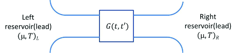
Figure 3: Theoretical scheme for Keldysh non-equilibrium Green function technique

In this review article, we give first a brief description of the Landauer-Büttiker approach Imry2002 ; Buttiker1992 , the non-equilibrium Green function technique Haug2008 ; Wingreen1993 ; Jauho1994 , and the master equation approach Tu2008 ; Tu2009 ; Jin2010 ; Schoeller1994 ; Gurvitz1996 ; Jin2008 ; Li2016 ; Yan2016 . The theoretical schemes of these approaches are schematically presented in Figs. 2, 3 and 6. The main differences between these three approaches are the ways of characterizing electron transport flowing through the device system. In the Landauer-Büttiker approach, the device system is depicted as a potential barrier, and all the information of the device system are imbedded in the scattering matrix. The actual structure of the device system is obscure. Comparing to the Landauer-Büttiker approach, the non-equilibrium Green function technique provides a more microscopic way by describing electrons flowing through the device system with single-particle non-equilibrium Green functions. In the master equation approach, the device system is described by the reduced density matrix, which is the essential quantity for studying quantum coherent and decoherent phenomena. Better than the non-equilibrium Green function in which the average over the density matrix has been done, quantum coherent dynamics is depicted explicitly by the off-diagonal matrix elements of the reduced density matrix. Then, in the subsequent sections, we will focus on applications of the master equation approach to various quantum transport problems in nanostructures. In particular, using master equation, we investigate transient current-current correlations and transient noise spectra for a quantum dot system which contain various time scales associated with the energy structures of the nanosystem (see Sec. III.1). The transient quantum transport in nanostructures is also investigated in the presence of initial correlations (see Sec. III.2). The relation of the phase dependence between the quantum states and the associated transport current are analyzed in a nanoscale Aharonov-Bohm (AB) interferometer, which provides an alternate possibility of quantum tomography in nanosystems (see Sec. III.3). At last, a conclusion is given in Sec. IV.

II Approaches for studying quantum transport in semiconductor nanostructures

II.1 Landauer-Büttiker approach

The Landauer-Büttiker formula has been widely utilized to calculate various transport properties in semiconductor nanostructures in the steady-state quantum transport regime Datta1995 ; Imry2002 . It establishes the fundamental relation between the electron wave functions (scattering amplitudes) of a quantum system and its conducting properties. In the Landauer-Büttiker formula, the transport current is given in terms of transmission coefficients, obtained from the single-particle scattering matrix. This approach is first formulated by Landauer for the single-channel transport Landauer1957 ; Landauer1970 . Later on, Büttiker et. al. extended the formula to multi-channel Buttiker1985 and multi-terminal cases Buttiker1986 . The further development of the Landauer-Büttiker approach is the calculation of the current noise correlations in mesoscopic conductors Buttiker1992 , the detailed discussion can be found from the review article by Blanter et. al. Blanter2000 .

A typical system considered in the Landauer-Büttiker approach consists of reservoirs (contacts), quantum leads, and a mesoscopic sample (scatterer) (see Fig. 2). The reservoirs connect to the mesoscopic sample by quantum leads, and are always in an equilibrium state in which electrons are always incoherent. However, electron transport passing through the mesoscopic sample between the reservoirs is phase coherent. Such coherent transport is described by the electron wave function scattered in the mesoscopic sample, which can be characterized by a scattering matrix $\bm{S}$. Therefore, the key to describe electron quantum transport in Landauer-Büttiker approach is to determine the scattering matrix $\bm{S}$ which relies crucially on the mesoscopic sample structure.

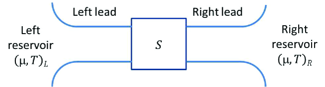
Figure 2: Theoretical scheme for scattering theory

We start with the single-channel and two-terminal case. Consider an electron plane wave impinging on a finite potential barrier from left ($x<0$), and is scattered into the reflected and transmitted components. Assume that the energy and momentum are conserved in the scattering process, and the wave function of the electron incident from the left and right are given respectively,

$$\psi_{L}(x)= \left\{\begin{array}[]{ll}e^{ikx}+re^{-ikx}&x<0,\\ te^{ikx}&x>0,\end{array}\right.$$ (3)

$$\psi_{R}(x)= \left\{\begin{array}[]{ll}t^{\prime}e^{-ikx}&x<0,\\ e^{-ikx}+r^{\prime}e^{ikx}&x>0,\end{array}\right.$$ (6)

where $r$ ($r^{\prime}$) and $t$ ($t^{\prime}$) are respectively the complex reflected and transmitted amplitudes of the wave incoming from the left (right), with $|r|^{2}$ ($|r^{\prime}|^{2}$) and $|t|^{2}$ ($|t^{\prime}|^{2}$) being the reflected and transmitted probabilities. These wave functions are the so-called scattering states. For a general incoming state, $a_{L}e^{ikx}+a_{R}e^{-ikx}$, with probability amplitudes $a_{L,R}$, the total wave function should be

$$\Psi(x)=\left\{\begin{array}[]{ll}a_{L}e^{ikx}+b_{L}e^{-ikx}&x<0,\\ a_{R}e^{-ikx}+b_{R}e^{ikx}&x>0,\end{array}\right.$$ (9)

by introducing probability amplitudes $b_{L,R}$ for the outgoing state such that the incoming and outgoing probability amplitudes are related to each other by the scattering matrix:

$$\left(\begin{array}[c]{cc}b_{L}\\ b_{R}\end{array}\right)=\left(\begin{array}[c]{cc}r&t^{\prime}\\ t&r^{\prime}\end{array}\right)\left(\begin{array}[c]{cc}a_{L}\\ a_{R}\end{array}\right)\equiv\bm{S}\left(\begin{array}[c]{cc}a_{L}\\ a_{R}\end{array}\right).$$ (18)

The coefficients in the scattering matrix ($r$, $t$, $r^{\prime}$, and $t^{\prime}$) are obtained by solving the Schrödinger equation with the potential that models the mesoscopic sample.

It is straightforward to generalize the formalism to multi-channel case where there are $N_{L}$ modes on the left and $N_{R}$ modes on the right. The incoming and outgoing amplitudes can be written in vectors such that

$$\bm{a}=\left(\begin{array}[c]{cc}a_{L1}\\ \vdots\\ a_{LN_{L}}\\ a_{R1}\\ \vdots\\ a_{RN_{R}}\end{array}\right);~{}~{}~{}~{}\bm{b}=\left(\begin{array}[c]{cc}b_{L1}\\ \vdots\\ b_{LN_{L}}\\ b_{R1}\\ \vdots\\ b_{RN_{R}}\end{array}\right),$$ (31)

and the scattering matrix, leading to $\bm{b}=\bm{S}\bm{a}$, is in dimension $(N_{L}+N_{R})\times(N_{L}+N_{R})$ and has the following form,

$$\bm{S}=\left(\begin{array}[c]{cc}\bm{s}_{LL}&\bm{s}_{LR}\\ \bm{s}_{RL}&\bm{s}_{RR}\end{array}\right)=\left(\begin{array}[c]{cc}\bm{r}&\bm{t}^{\prime}\\ \bm{t}&\bm{r}^{\prime}\end{array}\right),$$ (36)

where the matrices $\bm{t}$ ($N_{R}\times N_{L}$) and $\bm{r}$ ($N_{L}\times N_{L}$) describe respectively the transmission and reflection of electrons incoming from the left with the element $\bm{t}_{mn}$ and $\bm{r}_{mn}$ characterizing respectively the electrons transmitted from the left mode $n$ into the right mode $m$ and the electrons reflected from the left mode $n$ into the left mode $m$. Similarly, the matrices $\bm{r}^{\prime}$ ($N_{R}\times N_{R}$) and $\bm{t}^{\prime}$ ($N_{L}\times N_{R}$) represent the reflection and transmission processes for states incoming from the right. The scattering matrix $\bm{S}$ is unitary due to the flux conservation, i.e.

$$\bm{S}^{\dagger}\bm{S}=\bm{S}\bm{S}^{\dagger}=\mathds{1}.$$ (37)

Consider the Hamiltonian of lead $\alpha$ ($\alpha=L,R$),

$$H_{\alpha}=\frac{p^{2}_{x_{\alpha}}}{2m^{*}}+\frac{p^{2}_{\perp\alpha}}{2m^{*}}+U(\bm{r}_{\perp\alpha}),$$ (38)

where $x_{\alpha}$ and $\bm{r}_{\perp\alpha}$ denote the local coordinates in the longitudinal and transverse directions, respectively, and $m^{*}$ is the effective mass of the electron in the lead. The motion of electrons in the longitudinal direction is free, but it is quantized in the transverse direction due to the confinement potential $U(\bm{r}_{\perp\alpha})$. Then, the eigenfunctions of the Hamiltonian $H_{\alpha}$ can be expressed as

$$\phi^{\pm}_{\alpha n}(x_{\alpha},\bm{r}_{\perp\alpha})=\chi_{\alpha n}(\bm{r}_{\perp\alpha})e^{\pm ik_{\alpha n}x_{\alpha}},$$ (39)

where the incoming wave $e^{ikx_{\alpha}}$ and outgoing wave $e^{-ikx_{\alpha}}$ characterize the longitudinal motion of elections, and $\chi_{\alpha n}(\bm{r}_{\perp\alpha})$ satisfies

$$\big{[}~{}\frac{p^{2}_{\perp\alpha}}{2m^{*}}+U(\bm{r}_{\perp\alpha})~{}\big{]}\chi_{\alpha n}(\bm{r}_{\perp\alpha})=\epsilon_{\alpha n}\chi_{\alpha n}(\bm{r}_{\perp\alpha}),$$ (40)

with each transverse mode contributing a transport channel. As a result, the dispersion relation of electron is thus given by

$$E_{\alpha n}(k_{\alpha n})=\frac{\hbar^{2}k^{2}_{\alpha n}}{2m^{*}}+\epsilon_{\alpha n}.$$ (41)

In this case, for an electron from mode $m$ of lead $\alpha$ scattering by the mesoscopic sample, the scattering state of the electron for lead $\alpha$ is

$$\psi_{\alpha m}(\alpha)=\sum_{n}\big{\{}\delta_{mn}\phi^{+}_{\alpha n}+\sqrt{\frac{v_{\alpha m}}{v_{\alpha n}}}S_{\alpha\alpha nm}\phi^{-}_{\alpha n}\big{\}},$$ (42)

where $S_{\alpha\beta nm}$ represents the amplitude of a state scattered from mode $m$ in lead $\beta$ to mode $n$ in lead $\alpha$, and the factor $\sqrt{v_{\alpha m}/v_{\alpha n}}$ is introduced to guarantee the flux conservation, where $v_{\alpha m}=\hbar k_{\alpha m}/m^{*}$ is the electron velocity. The corresponding scattering state for lead $\beta\neq\alpha$ is

$$\psi_{\alpha m}(\beta)=\sum_{n}\sqrt{\frac{v_{\alpha m}}{v_{\beta n}}}S_{\beta\alpha nm}\phi^{-}_{\beta n}.$$ (43)

In the second quantization scheme, a general state of the lead-device system is given by an arbitrary superposition of these scattering states,

$$\hat{\Psi}(\bm{r},t)\!=\!\frac{1}{\sqrt{2\pi}}\!\!\sum_{\alpha m}\!\int\!\!dk_{\alpha m}\psi_{\alpha m}(\bm{r})e^{-\frac{i}{\hbar}E_{\alpha m}(k_{\alpha m})t}\hat{a}_{\alpha m}(k_{\alpha m}),$$ (44)

where $\hat{a}_{\alpha m}(k_{\alpha m})$ is the annihilation operator satisfying the canonical anti-commutation relation,

$$\big{\{}\hat{a}_{\alpha m}(k),\hat{a}^{\dagger}_{\beta n}(k^{\prime})\big{\}}=\delta_{\alpha\beta}\delta_{nm}\delta(k-k^{\prime}).$$ (45)

Changing the $k$ space into the energy space, and defining the incoming operator in the energy space $\hat{a}_{\alpha m}(E)=\hat{a}_{\alpha m}(k)/[\hbar v_{\alpha m}(k)]^{1/2}$, one has

$$\big{\{}\hat{a}_{\alpha m}(E),\hat{a}^{\dagger}_{\beta n}(E^{\prime})\big{\}}=\delta_{\alpha\beta}\delta_{nm}\delta(E-E^{\prime}),$$ (46)

where $\delta(E-E^{\prime})=1/v_{\alpha m}\delta(k-k^{\prime})$. The field operator can be rewritten as

$$\hat{\Psi}(\bm{r},t)=\sum_{\alpha m}\!\!\int\!\!\frac{dE_{\alpha m}}{\sqrt{hv_{\alpha m}(E_{\alpha m})}}\psi_{\alpha m}(\bm{r})e^{-\frac{i}{\hbar}E_{\alpha m}t}\hat{a}_{\alpha m}(E_{\alpha m}).$$ (47)

With the above solution, the current flowing from contact $\alpha$ to the mesoscopic sample can be deduced. The current operator of lead $\alpha$ is given by

$$\hat{I}_{\alpha}(t)=\int d\bm{r}_{\perp\alpha}\hat{j}(\bm{r}_{\alpha},t),$$ (48)

where the current density operator is expressed as

$$\hat{j}(\bm{r},t)=\frac{\hbar}{2m^{*}i}[\hat{\Psi}^{\dagger}\nabla\hat{\Psi}-(\nabla\hat{\Psi}^{\dagger})\hat{\Psi}].$$ (49)

Substituting the scattering states Eq. (42) and Eq. (43) into the field operator of Eq. (47) gives the following form,

$$\hat{\Psi}(\bm{r}_{\alpha},t)= \sum_{m}\!\int\!\!\frac{dE_{\alpha m}}{\sqrt{hv_{\alpha m}(E_{\alpha m})}}e^{-\frac{i}{\hbar}E_{\alpha m}t}\hat{a}_{\alpha m}(E_{\alpha m})$$

$$\times\Big{\{}\sum_{n}\big{[}\delta_{mn}\phi^{+}_{\alpha n}+\sqrt{\frac{v_{\alpha m}}{v_{\alpha n}}}S_{\alpha\alpha nm}\phi^{-}_{\alpha n}\big{]}$$

$$~{}~{}~{}~{}~{}~{}+\sum_{\beta\neq\alpha}\sum_{n}\sqrt{\frac{v_{\alpha m}}{v_{\beta n}}}S_{\beta\alpha nm}\phi^{-}_{\beta n}\Big{\}}$$

$$= \sum_{m}\!\int\!\!\frac{dE_{\alpha m}}{\sqrt{hv_{\alpha m}(E_{\alpha m})}}e^{-\frac{i}{\hbar}E_{\alpha m}t}$$

$$\times\Big{[}\phi^{+}_{\alpha m}\hat{a}_{\alpha m}(E_{\alpha m})+\phi^{-}_{\alpha m}\hat{b}_{\alpha m}(E_{\alpha m})\Big{]},$$ (50)

where the contribution of the incoming (the first term) and outgoing (the second term) states are explicitly presented in the above form. Using the orthogonal properties of different transverse modes, $\int d\bm{r}_{\perp\alpha}\chi_{\alpha m}(\bm{r}_{\perp\alpha})\chi_{\alpha n}(\bm{r}_{\perp\alpha})=\delta_{mn}$, the current can be reduced to the following form,

$$\hat{I}_{\alpha}(t)=\frac{e}{h}\sum_{m}\!\int\!\! dEdE^{\prime}\big{[}\hat{a}^{\dagger}_{\alpha m}(E)\hat{a}_{\alpha m}(E^{\prime})$$

$$-\hat{b}^{\dagger}_{\alpha m}(E)\hat{b}_{\alpha m}(E^{\prime})\big{]}e^{i(E-E^{\prime})t/\hbar},$$ (51)

with the approximation $v_{\alpha m}(E)=v_{\alpha m}(E^{\prime})$ which is always valid for a slowly-varying function $v(E)$. From the scattering relation $\bm{b}=\bm{S}\bm{a}$, one can express the current as

$$\hat{I}_{\alpha}(t)\!=\!\frac{e}{h}\!\!\sum_{\beta\gamma nk}\!\!\int\!\!dEdE^{\prime}\hat{a}^{\dagger}_{\beta n}\!(\!E)A^{nk}_{\beta\gamma}(\!\alpha;\!E,\!E^{\prime}\!)\hat{a}_{\gamma k}(\!E^{\prime}\!)e^{\frac{i}{\hbar}(\!E-E^{\prime}\!)t}$$ (52)

with the matrix $A$ having the following form

$$A^{nk}_{\beta\gamma}(\alpha;E,E^{\prime})=\delta_{\alpha\beta}\delta_{\alpha\gamma}\delta_{kn}-\sum_{m}S^{\dagger}_{\alpha\beta nm}(E)S_{\alpha\gamma mk}(E^{\prime}).$$ (53)

Because contact $\alpha$ is in equilibrium, the average current at lead $\alpha$ is then,

$$\langle I_{\alpha}\rangle=\frac{e}{h}\sum_{\beta n}\int dEA^{nn}_{\beta\beta}(\alpha,E,E)f_{\beta}(E),$$ (54)

where $f_{\alpha}(E)=1/(e^{(E-\mu_{\alpha})/k_{B}T_{\alpha}}+1)$ is the Fermi-Dirac distribution of contact $\alpha$ at the chemical potential $\mu_{\alpha}$ and temperature $T_{\alpha}$. Applying with the scattering matrix (36), the average current of the left lead becomes

$$\langle I_{L}\rangle=\frac{e}{h}\int dE~{}{\rm Tr}[\bm{t}^{\dagger}(E)\bm{t}(E)][f_{L}(E)-f_{R}(E)].$$ (55)

This gives the famous Landauer-Büttiker formula Buttiker1992 . Here, $\bm{t}(E)=\bm{t}^{\prime}(E)$ coming from the time-reversal symmetry.

In the steady-state quantum transport regime, the Landauer-Büttiker approach is a powerful method to calculate various transport properties in semiconductor nanostructures Buttiker1988 ; Buttiker1990 ; Samuelsson2006 ; Rothstein2009 . However, the scattering theory considers the reservoirs connecting to the scatterer (the mesoscopic sample) to be always in equilibrium and electrons in the reservoir are always incoherent. Thus, the Landauer-Büttiker formula becomes invalid to transient quantum transport. The scattering theory method could be extended to deal with time-dependent transport phenomena, through the so-called the Floquet scattering theory Moskalets2004 ; Wohlman2002 ; Moskalets2007 , but it is only applicable to the case of the time-dependent quantum transport for systems driven by periodic time-dependent external fields.

II.2 Non-equilibrium Green function technique

Green function techniques are widely used in many-body systems. For equilibrium systems, zero temperature Green functions and Matsubara (finite temperature) Green functions are useful tools for calculating the thermodynamical properties of many-body systems, as well as the linear responses of systems under small time-dependent (or not) perturbations Mahan1990 . However, when systems are driven out of equilibrium, non-equilibrium Green functions are utilized Haug2008 ; Wingreen1993 ; Jauho1994 . Non-equilibrium Green function techniques are initiated by Scwinger Schwinger1961 and Kadanoff and Baym Kadanoff1962 , and popularized by Keldysh Keldysh1965 . To deal with non-equilibrium phenomena, the contour-ordered Green functions which are defined on complex time contours are introduced such that the equations of motion and perturbation expansions of contour-ordered Green functions are formally identical to that of usual equilibrium Green functions.

In this section, the contour-ordered Green functions defined on Kadanoff-Baym contour which takes into account the initial correlations and statistical boundary conditions will be discussed. The real-time non-equilibrium Green functions are deduced from the contour-ordered Green function by analytic continuation. In application, one gives a detailed derivation of the transport current for a mesoscopic system by means of the Keldysh technique. The resulting transport current is formulating in terms of the non-equilibrium Green functions of the device system, which provides a more microscopic picture to the electron transport, in comparison to the Landauer-Büttiker formula, see Fig. 6. For a more complete description of non-equilibrium Green function techniques, we refers the readers to Haug2008 ; Kadanoff1962 ; Stefanucci2004 .

The contour-ordered Green function of non-equilibrium many-body theory is defined as,

$$G(\bm{x},\tau;\bm{x}^{\prime},\tau^{\prime}) \!=\!-i\langle T_{C}[\psi(\bm{x},\tau)\psi^{\dagger}(\bm{x}^{\prime},\tau^{\prime})]\rangle$$

$$\!=\!-i{\rm Tr}\big{[}\rho_{tot}(t_{0})T_{C}\!\big{\{}\psi(\bm{x},\tau)\psi^{\dagger}(\bm{x}^{\prime}\!,\!\tau^{\prime})\!\big{\}}\big{]},$$ (56)

where $\psi(\bm{x},\tau)$ and $\psi^{\dagger}(\bm{x}^{\prime},\tau^{\prime})$ are the fermion field operators in the Heisenberg picture with time variables $\tau$,$\tau^{\prime}$ (denoted by Greek letters) defined on the complex contour $C$, and $T_{C}$ is a contour-ordering operator which orders the operators according to their time labels on the contour:

$$T_{C}[\psi(\bm{x},\tau)\psi^{\dagger}(\bm{x}^{\prime},\tau^{\prime})]\equiv\left\{\begin{array}[]{ll}\psi(\bm{x},\tau)\psi^{\dagger}(\bm{x}^{\prime},\tau^{\prime})&\tau>_{C}\tau^{\prime},\\ -\psi^{\dagger}(\bm{x}^{\prime},\tau^{\prime})\psi(\bm{x},\tau)&\tau<_{C}\tau^{\prime}.\end{array}\right.$$ (59)

From the above definition, it is straightforward to rewrite the contour-ordered Green function as,

$$G(\bm{x},\tau;\bm{x}^{\prime},\tau^{\prime})= \Theta_{C}(\tau-\tau^{\prime})G^{>}(\bm{x},\tau;\bm{x}^{\prime},\tau^{\prime})$$

$$+\Theta_{C}(\tau^{\prime}-\tau)G^{<}(\bm{x},\tau;\bm{x}^{\prime},\tau^{\prime}),$$ (60)

where $\Theta_{C}(\tau-\tau^{\prime})$ is the step function defined on the contour in a clockwise direction, and $G^{>}$ and $G^{<}$ are the greater and lesser Green functions, respectively. The configuration of complex contour $C$ is determined by the initial density matrix of the total system $\rho_{tot}(t_{0})$.

The non-equilibrium dynamics considered in the Kadanoff-Baym formalism is formulated as follows. The physical system is described by a time-independent Hamiltonian,

$$h=H_{0}+H_{i},$$ (61)

where $H_{0}$ represents a free Hamiltonian, and $H_{i}$ is the interaction between the particles. The system is initially assumed at thermal equilibrium, which means the system is in partition-free scheme Cini1980 ,

$$\rho_{tot}(t_{0})=\frac{\exp(-\beta h)}{{\rm Tr}[\exp(-\beta h)]}=\frac{1}{Z}\exp(-\beta h),$$ (62)

where $\beta=1/k_{B}T$, and the particle energies are measured from the chemical potential $\mu$. After $t=t_{0}$, the system is exposed to external disturbances, e.g. an electric field, a light excitation pulse, or a coupling to contacts at differing (electro) chemical potentials that are described by time-dependent Hamiltonian $H^{\prime}(t)$. Thus, the total Hamiltonian is,

$$H(t)=h+H^{\prime}(t),$$ (63)

where $H^{\prime}(t<t_{0})=0$. By choosing the time arguments in contour-ordered Green function (II.2) are real time variables $t$ and $t^{\prime}$, the field operator $\psi(\bm{x},t)$ is then,

$$\psi(\bm{x},t)\equiv\psi(1)=\mathcal{U}(t_{0},t)\hat{\psi}_{h}(1)\mathcal{U}(t,t_{0}),$$ (64)

where the shorthand notation $(1)=(\bm{x},t)$ has been used, and $\mathcal{U}$ is the evolution operator for the time-dependent Hamiltonian $H^{\prime}(t)$,

$$\mathcal{U}(t,t^{\prime})=T\big{\{}\exp\big{[}-i\int^{t}_{t^{\prime}}dt_{1}\hat{H}^{\prime}_{h}(t_{1})\big{]}\big{\}}.$$ (65)

In the above equations, $\hat{\psi}_{h}(1)$ and $\hat{H}^{\prime}_{h}(t)$ are operators in the interaction picture with respect to Hamiltonian $h$,

$$\hat{\psi}_{h}(1)= ~{}e^{ih(t-t_{0})}\psi(\bm{x},t_{0})e^{-ih(t-t_{0})},$$ (66a)

$$\hat{H}^{\prime}_{h}(t)= ~{}e^{ih(t-t_{0})}H^{\prime}(t)e^{-ih(t-t_{0})}.$$ (66b)

The contour-ordered Green function in Kadanoff-Baym formalism is now written as

$$iG(\!1,\!1^{\prime}\!)\!= {\rm Tr}\big{[}\rho_{tot}(t_{0}\!)T_{C}\big{\{}\mathcal{U}(t_{0},\!t\!)\hat{\psi}_{h}(1)\mathcal{U}(t,t^{\prime}\!)\hat{\psi}^{\dagger}_{h}(1^{\prime}\!)\mathcal{U}(t^{\prime}\!,\!t_{0}\!)\!\big{\}}\big{]}$$

$$= {\rm Tr}\big{[}\rho_{tot}(t_{0})T_{C_{0}}\big{\{}\mathcal{U}_{C_{0}}(t_{0},t_{0})\hat{\psi}_{h}(1)\hat{\psi}^{\dagger}_{h}(1^{\prime})\!\big{\}}\big{]},$$ (67)

where $\mathcal{U}_{C_{0}}(t_{0},t_{0})=T_{C_{0}}\{\exp[-i\oint_{C_{0}}d\tau_{1}\hat{H}^{\prime}_{h}(\tau_{1})]\}$ is the evolution operator defined on the close path contour $C_{0}$ as shown in Fig. 4.

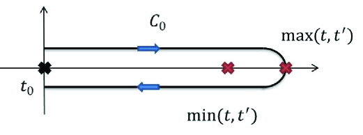
Figure 4: Closed time path contour $C_{0}$

In order to perform the Wick theorem, one needs to further transform the operators $\hat{\psi}_{h}(1)$, $\hat{\psi}^{\dagger}_{h}(1^{\prime})$ in the interaction picture with respect to the free Hamiltonian $H_{0}$:

$$\hat{\psi}_{h}(1)=U(t_{0},t)\hat{\psi}(1)U(t,t_{0}).$$ (68)

Here, $U$ being the evolution operator for the interaction Hamiltonian $H_{i}$,

$$U(t,t^{\prime})=T\big{\{}\exp\big{[}-i\int^{t}_{t^{\prime}}dt_{1}\hat{H}_{i}(t)\big{]}\big{\}},$$ (69)

and $\hat{\psi}(1)$ and $\hat{H}_{i}(t)$ in the interaction picture are given by,

$$\hat{\psi}(1)= e^{iH_{0}(t-t_{0})}\psi(\bm{x},t_{0})e^{-iH_{0}(t-t_{0})},$$ (70a)

$$\hat{H}_{i}(t)= e^{iH_{0}(t-t_{0})}H_{i}e^{-iH_{0}(t-t_{0})}.$$ (70b)

Furthermore, one can rewrite the factor $\exp(-\beta h)$ in the initial density matrix,

$$\exp(-\beta h)=\exp(-\beta H_{0})U(t_{0}-i\beta,t_{0}).$$ (71)

Finally, the contour-ordered Green function is reduced to,

$$iG(1,1^{\prime}\!)= \frac{{\rm Tr}\big{\{}\rho_{0}T_{C^{*}_{0}}\big{[}U_{C^{*}_{0}}(t_{0}\!-\!i\beta,t_{0})\mathcal{U}_{C_{0}}(t_{0},t_{0})\hat{\psi}(1\!)\hat{\psi}^{\dagger}(1^{\prime})\big{]}\!\big{\}}}{{\rm Tr}\big{\{}\rho_{0}T_{C^{*}_{0}}\big{[}U_{C^{*}_{0}}(t_{0}-i\beta,t_{0})\mathcal{U}_{C_{0}}(t_{0},t_{0})\big{]}\big{\}}},$$ (72)

where $\rho_{0}=e^{-\beta H_{0}}/Z_{0}$ is the equilibrium density matrix of Hamiltonian $H_{0}$, and $U_{C^{*}_{0}}(t_{0}-i\beta,t_{0})=T_{C^{*}_{0}}\{\exp[-i\int_{C^{*}_{0}}d\tau_{1}\hat{H}_{i}(\tau_{1})]\}$ is the evolution operator defined on contour $C^{*}_{0}=C_{0}\cup[t_{0},t_{0}-i\beta]$ which is the Kadanoff-Baym contour shown in Fig. 5.

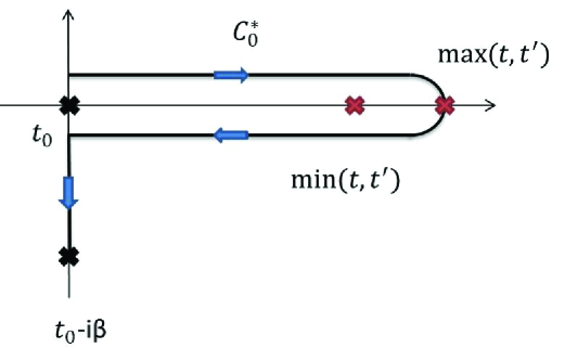
Figure 5: Kadanoff-Baym contour $C^{*}_{0}$

Eq. (72) is the exact contour-ordered Green function in Kadanoff-Baym formalism, which is defined in the interaction picture with respect to the free Hamiltonian $H_{0}$, so that Wick theorem is always applicable. Thus, the perturbative evaluation of Eq. (72) could be put in a form analogous to the usual Feynman diagrammatic technique as in the equilibrium Green function techniques, which leads to the Keldysh formalism.

On the other hand, the contour-ordered Green function obeys the following Dyson equation,

$$G(1,1^{\prime})=G_{0}(1,1^{\prime})+\!\!\int\!\!d2\!\!\int\!\!d3G_{0}(1,2)\Sigma(2,3)G(3,1^{\prime}),$$ (73a)

$$G(1,1^{\prime})=G_{0}(1,1^{\prime})+\!\!\int\!\!d2\!\!\int\!\!d3G(1,2)\Sigma(2,3)G_{0}(3,1^{\prime}),$$ (73b)

where $G_{0}(1,1^{\prime})=-i\langle T_{C}[\hat{\psi}(1)\hat{\psi}^{\dagger}(1^{\prime})]\rangle$ is the unperturbed Green function, $\Sigma(2,3)$ is the one particle irreducible self-energy, and the integral sign $\int d2(3)$ denotes a sum over all integral variables. The equations can be simply written as,

$$G=G_{0}+G_{0}\Sigma G,$$ (74a)

$$G=G_{0}+G\Sigma G_{0}.$$ (74b)

The Dyson equation can be regarded as the Schrödinger equation of a particle in the medium subject to the self-energy as the potential. In the Dyson equation, the single-particle Green function is entirely determined by the self-energy which contains all the many-body effects.

The steady-state transport current in a mesoscopic system is presented by the Keldysh formalism. Consider a nanostructure consisting of a quantum device coupled with two leads (the source and drain), which can be described by the Fano-Anderson Hamiltonian Fano1961 ; Anderson1958 ; Mahan1990 ,

$$H=\sum_{ij}\varepsilon_{ij}a_{i}^{{\dagger}}a_{j}+\sum_{\alpha k}\epsilon_{\alpha k}c_{\alpha k}^{{\dagger}}c_{\alpha k}$$

$$+\sum_{i\alpha k}[V_{i\alpha k}a^{{\dagger}}_{i}c_{\alpha k}+{\rm H.c.}].$$ (75)

Here $a_{i}^{{\dagger}}$ ($a_{i}$) and $c_{\alpha k}^{{\dagger}}$ ($c_{\alpha k}$) are creation (annihilation) operators of electrons in the quantum device and lead $\alpha$, respectively, $\varepsilon_{ij}$ and $\epsilon_{\alpha k}$ are the corresponding energy levels, $V_{i\alpha k}$ is the tunneling amplitude between the orbital state $i$ of the device system and the orbital state $k$ of lead $\alpha$. In the Keldysh approach, the quantum device and the leads are decoupled in the remote past, and the tunneling between them is viewed as a perturbation. Then, the time-independent Hamiltonian $h$, time-dependent Hamiltonian $H^{\prime}(t)$, and the initial density matrix $\rho_{tot}(-\infty)$ of the total system are,

$$h=H_{0}=\sum_{ij}\varepsilon_{ij}a_{i}^{{\dagger}}a_{j}+\sum_{\alpha k}\epsilon_{\alpha k}c_{\alpha k}^{{\dagger}}c_{\alpha k},$$ (76a)

$$H^{\prime}(t>t_{0})=\sum_{i\alpha k}[V_{i\alpha k}a^{{\dagger}}_{i}c_{\alpha k}+{\rm H.c.}],$$ (76b)

$$\rho_{tot}(-\infty)=\rho_{L}\otimes\rho(-\infty)\otimes\rho_{R},$$ (76c)

where $H_{\alpha}=\sum_{k}\epsilon_{\alpha k}c^{\dagger}_{\alpha k}c_{\alpha k}$ and $N_{\alpha}=\sum_{k}c^{\dagger}_{\alpha k}c_{\alpha k}$ are the Hamiltonian and the total particle number of lead $\alpha$, respectively. Lead $\alpha$ is initially in thermal equilibrium $\rho_{\alpha}=\frac{1}{Z}\big{[}e^{-\beta_{\alpha}(H_{\alpha}-\mu_{\alpha}N_{\alpha})}\big{]}$ with inverse temperature $\beta_{\alpha}$ and chemical potential $\mu_{\alpha}$. The device system can be in an arbitrary state $\rho(-\infty)$, i.e. the total system is in the partitioned scheme Caroli1971a ; Caroli1971b .

In non-equilibrium Green function techniques, the information of the dissipation and fluctuation dynamics of the device system can be extracted from the contour-ordered Green function of the device system $G_{ij}(\tau,\tau^{\prime})$,

$$G_{ij}(\tau,\tau^{\prime})= -i\langle T_{C}[a_{i}(\tau)a^{\dagger}_{j}(\tau^{\prime})]\rangle$$

$$= \Theta_{C}(\tau-\tau^{\prime})G^{>}_{ij}(\tau,\tau^{\prime})+\Theta_{C}(\tau^{\prime}-\tau)G^{<}_{ij}(\tau,\tau^{\prime}).$$ (77)

This Green function obeys the following equations of motion,

$$\sum_{l} \Big{[}i\frac{\partial}{\partial\tau}\delta_{il}-\varepsilon_{il}\Big{]}G_{lj}(\tau,\tau^{\prime})$$

$$=\delta_{C}(\tau-\tau^{\prime})\delta_{ij}+\sum_{\alpha k}V_{i\alpha k}G_{\alpha k,j}(\tau,\tau^{\prime}),$$ (78a)

$$\sum_{l} \Big{[}-i\frac{\partial}{\partial\tau^{\prime}}\delta_{lj}-\varepsilon_{lj}\Big{]}G_{il}(\tau,\tau^{\prime})$$

$$=\delta_{C}(\tau-\tau^{\prime})\delta_{ij}+\sum_{\alpha k}G_{i,\alpha k}(\tau,\tau^{\prime})V^{*}_{j\alpha k},$$ (78b)

where the mixed contour-ordered Green functions, $G_{\alpha k,j}(\tau,\tau^{\prime})=-i\langle T_{C}[c_{\alpha k}(\tau)a^{\dagger}_{j}(\tau^{\prime})]\rangle$ and $G_{i,\alpha k}(\tau,\tau^{\prime})=-i\langle T_{C}[a_{i}(\tau)c^{\dagger}_{\alpha k}(\tau^{\prime})]\rangle$, are given as follows

$$G_{i,\alpha k}(\tau,\tau^{\prime})= \sum_{l}\int_{C}d\tau_{1}G_{il}(\tau,\tau_{1})V_{l\alpha k}g_{\alpha k}(\tau_{1},\tau^{\prime}),$$ (79a)

$$G_{\alpha k,j}(\tau,\tau^{\prime})= \sum_{l}\int_{C}d\tau_{1}g_{\alpha k}(\tau,\tau_{1})V^{*}_{l\alpha k}G_{lj}(\tau_{1},\tau^{\prime}).$$ (79b)

Inserting Eq. (79a) and (79b) into Eq. (78) gives the Dyson equation in the differential form, i.e. Kadanoff-Byam equation,

$$[i\partial_{\tau}\mathds{1}_{D}-\bm{\varepsilon}]\bm{G}(\tau,\tau^{\prime}) =\mathds{1}_{D}\delta_{C}(\tau-\tau^{\prime})$$

$$+\int_{C}d\tau_{1}\bm{\Sigma}(\tau,\tau_{1})\bm{G}(\tau_{1},\tau^{\prime})$$ (80a)

$$\bm{G}(\tau,\tau^{\prime})[-i\partial_{\tau^{\prime}}\mathds{1}_{D}-\bm{\varepsilon}] =\mathds{1}_{D}\delta_{C}(\tau-\tau^{\prime})$$

$$+\int_{C}d\tau_{1}\bm{G}(\tau,\tau_{1})\bm{\Sigma}(\tau_{1},\tau^{\prime}),$$ (80b)

with self energy,

$$\Sigma_{ij}(\tau,\tau^{\prime})=\sum_{\alpha}\Sigma_{\alpha ij}(\tau,\tau^{\prime})=\sum_{\alpha k}V_{i\alpha k}g_{\alpha k}(\tau,\tau^{\prime})V^{*}_{j\alpha k}.$$ (81)

Here, $\mathds{1}_{D}$ is an identity matrix in the dimension of the device system. On the other hand, the equation of unperturbed contour-ordered Green function of the device system is,

$$[i\partial_{\tau}\mathds{1}_{D}-\bm{\varepsilon}]\bm{G}_{0}(\tau,\tau^{\prime})=\mathds{1}_{D}\delta_{C}(\tau-\tau^{\prime})$$ (82a)

$$\bm{G}_{0}(\tau,\tau^{\prime})[-i\partial_{\tau^{\prime}}\mathds{1}_{D}-\bm{\varepsilon}]=\mathds{1}_{D}\delta_{C}(\tau-\tau^{\prime}).$$ (82b)

Consequently, the Dyson equation (80) can be rewritten in the following form,

$$\bm{G}^{-1}_{0}\bm{G}=\mathds{1}+\bm{\Sigma}\bm{G},$$ (83a)

$$\bm{G}\bm{G}^{-1}_{0}=\mathds{1}+\bm{G}\bm{\Sigma}.$$ (83b)

Here, the matrix product means a product of all the internal variables (energy level and time). Equation (83) reproduces the integral form of Dyson equation (74).

Using the Dyson equation (74) and the Langreth theorem Langreth1976 , one has

$$\bm{G}^{R,A}=\bm{G}^{R,A}_{0}+\bm{G}^{R,A}_{0}\bm{\Sigma}^{R,A}\bm{G}^{R,A},$$ (84a)

$$\bm{G}^{\gtrless}=\bm{G}^{\gtrless}_{0}+\bm{G}^{R}_{0}\bm{\Sigma}^{R}\bm{G}^{\gtrless}+\bm{G}^{R}_{0}\bm{\Sigma}^{\gtrless}\bm{G}^{A}+\bm{G}^{\gtrless}_{0}\bm{\Sigma}^{A}\bm{G}^{A}.$$ (84b)

One can further iterates Eq. (84b) respect to $\bm{G}^{\gtrless}$ and obtains,

$$\bm{G}^{\gtrless}= (1\!+\!\bm{G}^{R}_{0}\bm{\Sigma}^{R})\bm{G}^{\gtrless}_{0}(1\!+\!\bm{\Sigma}^{A}\bm{G}^{A})$$

$$\!+\!(\bm{G}^{R}_{0}\!+\!\bm{G}^{R}_{0}\bm{\Sigma}^{R}\bm{G}^{R}_{0})\bm{\Sigma}^{\gtrless}\bm{G}^{A}\!+\!\bm{G}^{R}_{0}\bm{\Sigma}^{R}\bm{G}^{R}_{0}\bm{\Sigma}^{R}\bm{G}^{\gtrless}.$$ (85)

After iterates infinite orders, one can get,

$$\bm{G}^{\gtrless}=(1+\bm{G}^{R}\bm{\Sigma}^{R})\bm{G}^{\gtrless}_{0}(1+\bm{\Sigma}^{A}\bm{G}^{A})+\bm{G}^{R}\bm{\Sigma}^{\gtrless}\bm{G}^{A}.$$ (86)

In the Keldysh technique, the first term is neglected because it usually vanishes at steady-state limit. Then,

$$\bm{G}^{\gtrless}=\bm{G}^{R}\bm{\Sigma}^{\gtrless}\bm{G}^{A}.$$ (87)

Eq. (84a) and Eq. (87) are the final results of real time non-equilibrium Green functions in the Keldysh formalism which all the transport properties are determined by.

The transport current from lead $\alpha$ to the device system is defined as,

$$I_{\alpha}(t) \equiv-e\frac{d}{dt}\langle N_{\alpha}(t)\rangle=-\frac{ie}{\hbar}\langle[H,N_{\alpha}]\rangle$$

$$=\frac{2e}{\hbar}{\rm Re}\sum_{ik}V^{*}_{i\alpha k}G^{<}_{i,\alpha k}(t,t),$$ (88)

where the mixed lesser Green function, $G^{<}_{i,\alpha k}(t,t^{\prime})=i\langle c^{\dagger}_{\alpha k}(t^{\prime})a_{i}(t)\rangle$, can be obtained by applying the Langreth theorem to the mixed contour-ordered Green function (79a),

$$G^{<}_{i,\alpha k}(t,t^{\prime})=\sum_{j}\int^{\infty}_{-\infty} \!\!\!dt_{1}\big{[}G^{R}_{ij}(t,t_{1})V_{j\alpha k}g^{<}_{\alpha k}(t_{1},t^{\prime})$$

$$+G^{<}_{ij}(t,t_{1})V_{j\alpha k}g^{A}_{\alpha k}(t_{1},t^{\prime})\big{]}.$$ (89)

In the steady-state limit, all the Green functions usually depend on the differences of time arguments, i.e. $G(t,t^{\prime})=G(t-t^{\prime})$ because of time translation symmetry. Thus Green function $G^{<}_{i,\alpha k}(t,t)$ in the frequency domain can be expressed as,

$$G^{<}_{i,\alpha k}(t,t)=\sum_{j}\int\frac{d\omega}{2\pi} \big{[}G^{R}_{ij}(\omega)V_{j\alpha k}g^{<}_{\alpha k}(\omega)$$

$$+G^{<}_{ij}(\omega)V_{j\alpha k}g^{A}_{\alpha k}(\omega)\big{]},$$ (90)

Combinding Eq. (II.2) and (II.2), the steady-state transport current reduces to,

$$I_{\alpha}\!=\!\frac{ie}{\hbar}\!\int\!\!\frac{d\omega}{2\pi}{\rm Tr}\bm{\Gamma}_{\alpha}(\omega)\big{\{}f_{\alpha}(\omega)[\bm{G}^{R}(\omega)\!-\!\bm{G}^{A}(\omega)]\!+\!\bm{G}^{<}(\omega)\big{\}},$$ (91)

where $\Gamma_{\alpha ij}(\omega)=2\pi\sum_{k}V_{i\alpha k}V^{*}_{j\alpha k}\delta(\omega-\epsilon_{\alpha k})$ is a level-width function, and we have used the results of the free-particle Green functions given Haug2008 . Now, the transport current is fully determined by Green functions of the device system. Besides, for the non-interacting device system, one has,

$$\bm{G}^{R}(\omega)-\bm{G}^{A}(\omega) =\bm{G}^{>}(\omega)-\bm{G}^{<}(\omega)$$

$$=-i\bm{G}^{R}(\omega)\sum_{\alpha}\bm{\Gamma}_{\alpha}(\omega)\bm{G}^{A}(\omega).$$ (92)

Then, the steady-state transport current becomes,

$$I_{\alpha}=\frac{e}{\hbar}\sum_{\beta}\int\frac{d\omega}{2\pi}T_{\alpha\beta}(\omega)[f_{\alpha}(\omega)-f_{\beta}(\omega)],$$ (93)

where $T_{\alpha\beta}={\rm Tr}\big{[}\bm{\Gamma}_{\alpha}(\omega)\bm{G}^{R}(\omega)\bm{\Gamma}_{\beta}(\omega)\bm{G}^{A}(\omega)\big{]}$ is the transmission coefficient. This expression of the steady-state transport current reproduces the Landauer-Büttiker formula with the transmission probability being derived microscopically. The non-equilibrium Green function technique based on Keldysh formalism Schwinger1961 ; Keldysh1965 has been used extensively to investigate the steady-state quantum transport in mesoscopic systems Wingreen1993 ; Haug2008 ; Jauho1994 .

Wingreen et al. extended Keldysh’s non-equilibrium Green function technique to time-dependent quantum transport under time-dependent external bias and gate voltages Wingreen1993 ; Jauho1994 . Explicitly, the parameters in Hamiltonian (76), controlled by the external bias and gate voltages, become time dependent,

$$\varepsilon_{ij}\rightarrow\varepsilon_{ij}(t),$$ (94a)

$$\epsilon_{\alpha k}\rightarrow\epsilon_{\alpha k}(t)=\epsilon_{\alpha k}+\Delta_{\alpha k}(t),$$ (94b)

$$V_{i\alpha k}\rightarrow V_{i\alpha k}(t)$$ (94c)

Then, the time-dependent transport current becomes,

$$I_{\alpha}(t)=-\frac{2e}{\hbar}\!\!\int^{t}_{-\infty} \!\!\!d\tau\!\!\!\int\frac{d\omega}{2\pi}{\rm ImTr}\big{\{}e^{-i\omega(\tau-t)}\bm{\Gamma}_{\alpha}(\omega,\tau,t)$$

$$\times\big{[}f_{\alpha}(\omega)\bm{G}^{R}(t,\tau)+\bm{G}^{<}(t,\tau)\big{]}\big{\}},$$ (95)

where the level-width function is also time dependent,

$$\Gamma_{\alpha ij} (\omega,t_{1},t_{2})$$

$$= 2\pi\!\sum_{k}\!V_{i\alpha k}(t_{1})e^{\!-i\!\int^{t_{1}}_{t_{2}}ds\Delta_{\alpha k}(s)}V^{*}_{j\alpha k}(t_{2})\delta(\omega-\epsilon_{\alpha k}).$$ (96)

In particular, the Green functions in time domain are given by,

$$\bm{G}^{R}(t,t^{\prime}\!)\!\!=\!\bm{G}^{R}_{0}(t,t^{\prime})\!+\!\!\!\int\!\!dt_{1}\!\!\!\int\!\!\!dt_{2}\bm{G}^{R}_{0}(\!t,t_{1}\!)\bm{\Sigma}^{R}(\!t_{1},t_{2}\!)\bm{G}^{R}(\!t_{2},t^{\prime}\!),$$ (97a)

$$\bm{G}^{<}(t,t^{\prime})\!\!=\!\!\!\int\!\!dt_{1}\!\!\!\int\!\!\!dt_{2}\bm{G}^{R}(t,t_{1})\bm{\Sigma}^{<}(t_{1},t_{2})\bm{G}^{A}(t_{2},t^{\prime}).$$ (97b)

with self-energy defined as,

$$\Sigma^{R}_{ij}(t_{1},t_{2})\!=\!-i\Theta(t_{1}\!-\!t_{2})\!\!\sum_{\alpha}\!\!\int\!\!\frac{d\omega}{2\pi}\Gamma_{\alpha ij}(\omega,t_{1},t_{2})e^{-i\omega(t_{1}-t_{2})},$$ (98a)

$$\Sigma^{<}_{ij}(t_{1},t_{2})=i\sum_{\alpha}\int\frac{d\omega}{2\pi}f_{\alpha}(\omega)\bm{\Gamma}_{\alpha}(\omega,t_{1},t_{2})e^{-i\omega(t_{1}-t_{2})}$$ (98b)

This gives a general formalism for time-dependent current through the device system valid for non-linear response, where electron energies can be varied time-dependently by external gate voltages. However, in the Keldysh formalism, non-equilibrium Green functions are defined with the initial time $t_{0}\rightarrow-\infty$, where the initial correlations are hardly taken into account. This limits the Keldysh technique to be useful mostly in the non-equilibrium steady-state regime.

II.3 Master equation approach

The master equation approach concerns the dynamic properties of the device system in terms of the time evolution of the reduced density matrix $\rho(t)={\rm Tr_{E}}[\rho_{tot}(t)]$, where $\rm{Tr_{E}}$ is the trace over all the environmental (leads) degrees of freedom. The dissipation and fluctuation dynamics of the device system induced by the reservoirs (leads) are fully manifested in the master equation. The transient transport properties can be naturally addressed within the framework of the master equation. Compared to the non-equilibrium Green function technique, the master equation approach manifests the state information of the device system, see Fig. 6, which is a key element in studying quantum phenomena.

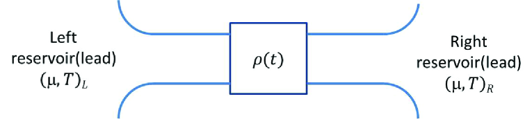
Figure 6: Theoretical scheme for master equation approach

In principle, the master equation for quantum transport can be solved in terms of the real-time diagrammatic expansion approach up to all orders Schoeller1994 . However, most of the master equations used in nanostructures are obtained by the perturbation theory up to the second order of the system-lead couplings, which is mainly applicable in the sequential tunneling regime Li2005 . A recent development of master equations in quantum transport systems is the hierarchical expansion of the equations of motion for the reduced density matrix Jin2008 ; Yan2016 , which provides a systematical and also very useful numerical calculation scheme for quantum transport.

A few years ago, we derived an exact master equation for non-interacting nanodevices Tu2008 ; Tu2009 ; Jin2010 , using the Feynman-Vernon influence functional approach Feynman1963 in the fermion coherent-state representation Zhang1990 . The obtained exact master equation not only describes the quantum state dynamics of the device system but also takes into account all the transient electronic transport properties. The transient transport current is obtained directly from the exact master equation Jin2010 , which turns out to be expressed precisely with the non-equilibrium Green functions of the device system Haug2008 ; Wingreen1993 ; Jauho1994 . This new theory has also been used to study quantum transport (including the transient transport) for various nanostructures recently Tu2008 ; Tu2009 ; Jin2010 ; Tu2011 ; Lin2011 ; Tu2012a ; Tu2012b ; Jin2013 ; Tu2014 ; Yang2014 ; Yang2015 ; Tu2016 ; Liu2016 . In the following, an introduction of this exact master equation approach Tu2008 ; Tu2009 ; Jin2010 is given, and the transient transport current derived using the exact master equation is explicitly presented.

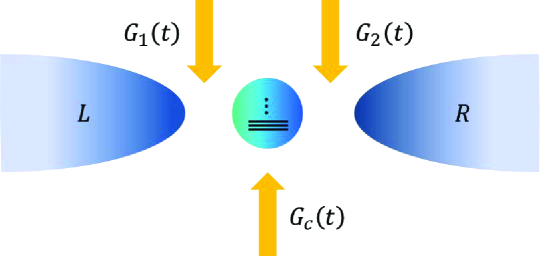
Figure 7: A schematic plot of a nanoscale quantum device in which the bias voltage is applied to the source and the drain electrode leads labeled $L$ and $R$, and other gates labeled $G_{c}$, $G_{1}$, $G_{2}$ control the energy levels of the central region as well as the couplings between the central region and the leads.

We begin with a nanostructure consisting of a quantum device coupled with two leads (the source and the drain), described by a time-dependent Fano-Anderson Hamiltonian Fano1961 ; Anderson1958 ; Mahan1990 ,

$$H(t)= H_{S}(t)+H_{E}(t)+H_{SE}(t),$$

with

$$H_{S}(t)=\sum_{ij}\bm{\varepsilon}_{ij}(t)a^{\dagger}_{i}a_{j},$$

$$H_{E}(t)=\sum_{\alpha k}\epsilon_{\alpha k}(t)c_{\alpha k}^{\dagger}c_{\alpha k},$$

$$H_{SE}(t)=\sum_{i\alpha k}\big{[}V_{i\alpha k}(t)a^{\dagger}_{i}c_{\alpha k}+V^{*}_{i\alpha k}(t)c_{\alpha k}^{\dagger}a_{i}\big{]},$$ (99)

where $a_{i}^{{\dagger}}$ ($a_{i}$) and $c_{\alpha k}^{{\dagger}}$ ($c_{\alpha k}$) are creation (annihilation) operators of electrons in the device system and lead $\alpha$, respectively; $\bm{\varepsilon}_{ij}(t)$ and $\epsilon_{\alpha k}(t)$ are the corresponding energy levels, and $V_{i\alpha k}(t)$ is the tunneling amplitude between the orbital state $i$ in the device system and the orbital state $k$ in lead $\alpha$. These time-dependent parameters in Eq. (II.3) can be manipulated by external bias and gate voltages in experiments (see Fig. 7).

The density matrix of the total system follows the unitary evolution,

$$\rho_{tot}(t)=\mathbf{U}(t,t_{0})\rho_{tot}(t_{0})\mathbf{U}^{\dagger}(t,t_{0}),$$ (100)

with the evolution operator $\mathbf{U}(t,t_{0})=T\exp\{-i\int^{t}_{t_{0}}H(\tau)d\tau\}$, where $T$ is the time-ordering operator. Here we assume, as usual, that the device system is uncorrelated with the reservoirs (leads) before the tunneling couplings are turned on Leggett1987 : $\rho_{tot}(t_{0})=\rho(t_{0})\otimes\rho_{E}(t_{0})$, in which the system can be in an arbitrary state $\rho(t_{0})$, and the reservoirs are initially in equilibrium, $\rho_{E}(t_{0})=\frac{1}{Z}e^{-\sum_{\alpha}\beta_{\alpha}(H_{\alpha}-\mu_{\alpha}N_{\alpha})}$, where $\beta_{\alpha}=1/(k_{B}T_{\alpha})$ is the inverse temperature of lead $\alpha$ at initial time $t_{0}$, and $N_{\alpha}=\sum_{k}c^{\dagger}_{\alpha k}c_{\alpha k}$ is the total particle number for lead $\alpha$. In other words, the system is in the so-called partitioned scheme Caroli1971a ; Caroli1971b as in the Keldysh framework. After $t_{0}$, the device system and the leads evolve into dynamically non-equilibrium states. These dynamically non-equilibrium processes are fully taken into account when we completely and exactly integrated over all the dynamical degrees of freedom of leads through the Feynman-Vernon influence functional. Here we do not need to specify or assume the lead distribution function after the initial time, since the quantum evolution operator of the total system (the dot, the leads and the coupling between them) in the Feynman-Vernon influence functional theory has automatically taken into account all possible states of the leads.

The non-equilibrium electron dynamics of an open system are determined by the reduced density matrix: $\rho(t)={\rm Tr_{E}}[\rho_{tot}(t)]$. In the fermion coherent-state representation Zhang1990 , the reduced density matrix at an arbitrary later time $t$ is expressed as,

$$\langle\bm{\xi}_{f}\!|\rho(t)\!|\bm{\xi}^{\prime}_{f}\rangle\!=\!\!\!\int\!\!\!d\mu(\bm{\xi}_{0}\!)d\mu(\!\bm{\xi}^{\prime}_{0}\!)\langle\bm{\xi}_{0}|\rho(t_{0})|\bm{\xi}^{\prime}_{0}\!\rangle\mathcal{J}\!(\bar{\bm{\xi}}_{f}\!,\!\bm{\xi}^{\prime}_{f}\!,\!t|\bm{\xi}_{0},\!\bar{\bm{\xi}}^{\prime}_{0},\!t_{0}),$$ (101)

with $\bm{\xi}=(\xi_{1},\xi_{2},...)$ and $\bar{\bm{\xi}}=(\xi^{*}_{1},\xi^{*}_{2},...)$ being the Grassmann variables and their complex conjugate defined through the fermion coherent states: $a_{i}|\bm{\xi}\rangle=\xi_{i}|\bm{\xi}\rangle$and $\langle\bm{\xi}|a^{\dagger}_{i}=\langle\bm{\xi}|\xi^{*}_{i}$. As these coherent states obey the completeness relation, $\int d\mu(\bm{\xi})|\bm{\xi}\rangle\langle\bm{\xi}|=\mathds{1}$, where the integration measure is defined by $d\mu(\bm{\xi})=\prod_{i}e^{-\xi^{*}_{i}\xi_{i}}d\xi^{*}_{i}d\xi_{i}$. The propagating function in equation (101) is given in terms of Grassmann variable path integrals,

$$\mathcal{J}\!(\bar{\bm{\xi}}_{f}\!,\!\bm{\xi}^{\prime}_{f}\!,\!t|\bm{\xi}_{0},\!\bar{\bm{\xi}}^{\prime}_{0},\!t_{0}\!)\! =\!\!\!\int\!\!\mathcal{D}[\bar{\bm{\xi}}\bm{\xi};\!\bar{\bm{\xi}}^{\prime}\!\bm{\xi}^{\prime}]e^{i(\!S_{c}[\bar{\bm{\xi}},\bm{\xi}]-S^{*}_{c}[\bar{\bm{\xi}}^{\prime}\!,\bm{\xi}^{\prime}])}\!\mathcal{F}[\bar{\bm{\xi}}\bm{\xi};\!\bar{\bm{\xi}}^{\prime}\!\bm{\xi}^{\prime}]$$

$$=\!\!\!\int\!\!\mathcal{D}[\bar{\bm{\xi}}\bm{\xi};\bar{\bm{\xi}}^{\prime}\bm{\xi}^{\prime}]e^{iS_{eff}[\bar{\bm{\xi}}\bm{\xi};\bar{\bm{\xi}}^{\prime}\bm{\xi}^{\prime}]},$$ (102)

where $S_{c}[\bar{\bm{\xi}},\bm{\xi}]$ and $S^{*}_{c}[\bar{\bm{\xi}}^{\prime}\bm{\xi}^{\prime}]$ are respectively the forward and backward actions of the device system in the fermion coherent-state representation. The influence functional $\mathcal{F}[\bar{\bm{\xi}}\bm{\xi};\bar{\bm{\xi}}^{\prime}\bm{\xi}^{\prime}]$ takes fully into account the back-action effects of the environments (leads) to the device system, it modifies the original action of the device system into an effective one, which dramatically changes the dynamics of the device system. After integrating out all the environmental degrees of freedom, the influence functional has the following form,

$$\mathcal{F}[\bar{\bm{\xi}} \bm{\xi};\bar{\bm{\xi}}^{\prime}\bm{\xi}^{\prime}]$$

$$= \!\exp\!\Big{\{}\!\!\!-\!\!\!\sum_{\alpha}\!\!\int^{t}_{t_{0}}\!\!\!d\tau\!\!\!\int^{\tau}_{t_{0}}\!\!\!\!d\tau^{\prime}\big{[}\bar{\bm{\xi}}(\!\tau\!)\bm{g}_{\alpha}(\!\tau,\!\tau^{\prime}\!)\bm{\xi}(\!\tau^{\prime}\!)\!+\!\bar{\bm{\xi}}^{\prime}(\!\tau^{\prime}\!)\bm{g}_{\alpha}(\!\tau^{\prime}\!,\!\tau\!)\bm{\xi}^{\prime}(\!\tau\!)\big{]}$$

$$~{}~{}~{}~{}~{}-\!\sum_{\alpha}\!\int^{t}_{t_{0}}\!\!d\tau\!\!\int^{t}_{t_{0}}\!\!d\tau^{\prime}\big{\{}\bar{\bm{\xi}}^{\prime}(\tau)\bm{g}_{\alpha}(\tau,\tau^{\prime})\bm{\xi}(\tau^{\prime})$$

$$~{}~{}~{}~{}~{}~{}~{}~{}~{}~{}~{}-[\bar{\bm{\xi}}(\tau)+\bar{\bm{\xi}}^{\prime}(\tau)]\widetilde{\bm{g}}_{\alpha}(\tau,\tau^{\prime})[\bm{\xi}(\tau^{\prime})+\bm{\xi}^{\prime}(\tau^{\prime})]\big{\}}\Big{\}}.$$ (103)

In the above equation, the time non-local integral kernels, $\bm{g}_{\alpha}(\tau,\tau^{\prime})$ and $\widetilde{\bm{g}}_{\alpha}(\tau,\tau^{\prime})$ characterize all the memory effects between the device system and lead $\alpha$,

$$\bm{g}_{\alpha ij}(\tau,\tau^{\prime})\!=\! \sum_{k}\!V_{i\alpha k}(\tau)V^{*}_{j\alpha k}(\tau^{\prime})e^{-i\!\int^{\tau}_{\tau^{\prime}}d\tau_{1}\epsilon_{\alpha k}(\tau_{1})}\!,$$ (104a)

$$\widetilde{\bm{g}}_{\alpha ij}(\tau,\tau^{\prime})\!=\! \sum_{k}\!V_{i\alpha k}(\tau)V^{*}_{j\alpha k}(\tau^{\prime})\!f_{\alpha}(\epsilon_{\alpha k})e^{-i\!\int^{\tau}_{\tau^{\prime}}d\tau_{1}\epsilon_{\alpha k}(\tau_{1})}\!,$$ (104b)

where $f_{\alpha}(\epsilon_{\alpha k})=1/(e^{\beta_{\alpha}(\epsilon_{\alpha k}-\mu_{\alpha})}+1)$ is the Fermi-Dirac distribution function of lead $\alpha$ at initial time $t_{0}$.

After integrating over all the forward paths $\bar{\bm{\xi}}(\tau)$, $\bm{\xi}(\tau)$ and the backward paths $\bar{\bm{\xi}}^{\prime}(\tau)$, $\bm{\xi}^{\prime}(\tau)$ in the Grassmann space bounded by $\bar{\bm{\xi}}(t)=\bar{\bm{\xi}}_{f}$, $\bm{\xi}(t_{0})=\bm{\xi}_{0}$, $\bar{\bm{\xi}}^{\prime}(t_{0})=\bar{\bm{\xi}}^{\prime}_{0}$, and $\bm{\xi}^{\prime}(t)=\bm{\xi}^{\prime}_{f}$, and by introducing a transformation,

$$\bm{\xi}(\tau)=\bm{u}(\tau,t_{0})\bm{\xi}(t_{0})+\bm{v}(\tau,t)[\bm{\xi}(t)+\bm{\xi}^{\prime}(t_{0})],$$ (105a)

$$\bm{\xi}(\tau)+\bm{\xi}^{\prime}(\tau)=\bm{u}^{\dagger}(t,\tau)[\bm{\xi}(t)+\bm{\xi}^{\prime}(t)],$$ (105b)

the propagating function becomes,

$$\mathcal{J}( \bar{\bm{\xi}}_{f},\bm{\xi}^{\prime}_{f},t|\bm{\xi}_{0},\bar{\bm{\xi}}^{\prime}_{0},t_{0})=\!\frac{1}{{\rm det}[\bm{w}(t)]}\!\exp\!\Big{\{}\!\bar{\bm{\xi}}_{f}\bm{J}_{1}(t)\bm{\xi}_{0}\!$$

$$+\!\bar{\bm{\xi}}_{f}\bm{J}_{2}(t)\bm{\xi}^{\prime}_{f}\!+\!\bar{\bm{\xi}}^{\prime}_{0}\bm{J}_{3}(t)\bm{\xi}_{0}\!+\!\bar{\bm{\xi}}^{\prime}_{0}\bm{J}^{\dagger}_{1}(t)\bm{\xi}^{\prime}_{f}\Big{\}},$$ (106)

where the time-dependent coefficients are given explicitly as,

$$\bm{J}_{1}(t)= \bm{w}(t)\bm{u}(t,t_{0}),~{}~{}~{}\bm{J}_{2}(t)=\bm{w}(t)-\mathds{1},$$

$$\bm{J}_{3}(t)= \bm{u}^{\dagger}(t,t_{0})\bm{w}(t)\bm{u}(t,t_{0})-\mathds{1},$$ (107)

with $\bm{w}(t)=[\mathds{1}-\bm{v}(t,t)]^{-1}$. As one can see, the propagating function is determined by the two Green functions $\bm{u}(t,t_{0})$ and $\bm{v}(t,t)$, which are $N_{S}\times N_{S}$ matrix with $N_{S}$ being the total number of single-particle energy levels in the device system. They satisfies the following integro-differential equations,

$$\frac{d}{d\tau}\bm{u}(\tau,t_{0})+i\bm{\varepsilon}(\tau)\bm{u}(\tau,t_{0})$$

$$~{}~{}~{}~{}~{}~{}~{}~{}~{}~{}~{}+\sum_{\alpha}\int_{t_{0}}^{\tau}d\tau^{\prime}\bm{g}_{\alpha}(\tau,\tau^{\prime})\bm{u}(\tau^{\prime},t_{0})=0,$$ (108a)

$$\frac{d}{d\tau}\bm{v}(\tau,t)+i\bm{\varepsilon}(\tau)\bm{v}(\tau,t)+\sum_{\alpha}\int_{t_{0}}^{\tau}d\tau^{\prime}\bm{g}_{\alpha}(\tau,\tau^{\prime})\bm{v}(\tau^{\prime},t)$$

$$~{}~{}~{}~{}~{}~{}~{}~{}~{}~{}~{}=\sum_{\alpha}\int_{t_{0}}^{t}d\tau^{\prime}\bm{\widetilde{g}}_{\alpha}(\tau,\tau^{\prime})\bm{u}^{{\dagger}}(t,\tau^{\prime}),$$ (108b)

subject to the boundary conditions $\bm{u}(t_{0},t_{0})=\mathds{1}$ and $\bm{v}(t_{0},t)=0$ with $t_{0}\leq\tau\leq t$. Actually, $\bm{u}(\tau,t_{0})$ and $\bm{v}(\tau,t)$ are related to the non-equilibrium Green functions of the device system as we will show later.

Taking the time derivative of the reduced density matrix (101) with the solution of the propagating function (II.3), together with the fermion creation and annihilation operator properties in the fermion coherent-state representation, one can obtain the final form of the exact master equation,

$${d\rho(t)\over dt}= \!-i\big{[}H^{\prime}_{S}(t),\rho(t)\big{]}\!\!+\!\!\sum_{ij}\!\big{\{}\bm{\gamma}_{ij}(t)\big{[}2a_{j}\rho(t)a_{i}^{{\dagger}}$$

$$-a_{i}^{{\dagger}}a_{j}\rho(t)-\rho(t)a_{i}^{{\dagger}}a_{j}\big{]}+\widetilde{\bm{\gamma}}_{ij}(t)\big{[}a_{i}^{{\dagger}}\rho(t)a_{j}$$

$$-a_{j}\rho(t)a_{i}^{{\dagger}}-\rho(t)a_{j}a_{i}^{{\dagger}}+a_{i}^{{\dagger}}a_{j}\rho(t)\big{]}\big{\}}$$

$$= -i\big{[}H_{S}(t),\rho(t)\big{]}+\sum_{\alpha}\big{[}\mathcal{L}^{+}_{\alpha}(t)+\mathcal{L}^{-}_{\alpha}(t)\big{]}\rho(t).$$ (109)

The first term describes the unitary evolution of electrons in the device system, where the renormalization effect, after integrating out all the lead degrees of freedom, has been fully taken into account. The resultant renormalized Hamiltonian is $H^{\prime}_{S}(t)=\sum_{ij}\varepsilon^{\prime}_{ij}(t)a_{i}^{{\dagger}}a_{j}$, with $\bm{\varepsilon}^{\prime}_{ij}(t)$ being the corresponding renormalized energy matrix of the device system, including the energy shift of each level and the lead-induced couplings between different levels. The remaining terms give the non-unitary dissipation and fluctuation processes induced by back-actions of electrons from the leads, and are described by the dissipation and fluctuation coefficients $\bm{\gamma}(t)$ and $\bm{\widetilde{\gamma}}(t)$, respectively. On the other hand, the current superoperators of lead $\alpha$, $\mathcal{L}^{+}_{\alpha}(t)$ and $\mathcal{L}^{-}_{\alpha}(t)$, determine the transport current flowing from lead $\alpha$ into the device system:

$$I_{\alpha}(t)= -e\Big{\langle}\frac{dN_{\alpha}(t)}{dt}\Big{\rangle}$$

$$= \frac{e}{\hbar}\rm{Tr}\big{[}\mathcal{L}^{+}_{\alpha}(t)\rho(t)\big{]}=-\frac{e}{\hbar}\rm{Tr}\big{[}\mathcal{L}^{-}_{\alpha}(t)\rho(t)\big{]},$$ (110)

where $N_{\alpha}(t)=\sum_{k}c^{\dagger}_{\alpha k}(t)c_{\alpha k}(t)$ is the total particle number of lead $\alpha$.

All the time-dependent coefficients in Eq. (II.3) are found to be,

$$\bm{\varepsilon}^{\prime}_{ij}(t)= \frac{i}{2}\big{[}\dot{\bm{u}}(t,t_{0})\bm{u}^{-1}(t,t_{0})-{\rm H.c.}\big{]}_{ij}$$

$$=\bm{\varepsilon}_{ij}(t)-\frac{i}{2}\sum_{\alpha}[\bm{\kappa}_{\alpha}(t)-\bm{\kappa}^{\dagger}_{\alpha}(t)]_{ij},$$ (111a)

$$\bm{\gamma}_{ij}(t)= -\frac{1}{2}\big{[}\dot{\bm{u}}(t,t_{0})\bm{u}^{-1}(t,t_{0})+{\rm H.c.}\big{]}_{ij}$$

$$=\frac{1}{2}\sum_{\alpha}[\bm{\kappa}_{\alpha}(t)+\bm{\kappa}^{\dagger}_{\alpha}(t)]_{ij},$$ (111b)

$$\widetilde{\bm{\gamma}}_{ij}(t)= \,\,\frac{d}{dt}\bm{v}_{ij}(t,t)-[\dot{\bm{u}}(t,t_{0})\bm{u}^{-1}(t,t_{0})\bm{v}(t,t)+{\rm H.c.}]_{ij}$$

$$=-\sum_{\alpha}[\bm{\lambda}_{\alpha}(t)+\bm{\lambda}^{\dagger}_{\alpha}(t)]_{ij},$$ (111c)

The current superoperators of lead $\alpha$, $\mathcal{L}^{+}_{\alpha}(t)$ and $\mathcal{L}^{-}_{\alpha}(t)$, are also explicitly given by

$$\!\mathcal{L}^{+}_{\alpha}(t)\rho(t)= -\!\!\sum_{ij}\big{\{}\bm{\lambda}_{\alpha ij}(t)\big{[}a^{\dagger}_{i}a_{j}\rho(t)+a^{\dagger}_{i}\rho(t)a_{j}\big{]}$$

$$+\bm{\kappa}_{\alpha ij}(t)a^{\dagger}_{i}a_{j}\rho(t)+\rm H.c.\big{\}},$$ (112a)

$$\!\mathcal{L}^{-}_{\alpha}(t)\rho(t)= \sum_{ij}\big{\{}\bm{\lambda}_{\alpha ij}(t)\big{[}a_{j}\rho(t)a^{\dagger}_{i}+\rho(t)a_{j}a^{\dagger}_{i}\big{]}$$

$$+\bm{\kappa}_{\alpha ij}(t)a_{j}\rho(t)a^{\dagger}_{i}+\rm H.c.\big{\}}.$$ (112b)

The functions $\bm{\kappa}_{\alpha}(t)$ and $\bm{\lambda}_{\alpha}(t)$ in Eq. (111) and Eq. (112) are solved from Eq. (108),

$$\bm{\kappa}_{\alpha}(t)= \int^{t}_{t_{0}}d\tau\bm{g}_{\alpha}(t,\tau)\bm{u}(\tau,t_{0})[\bm{u}(t,t_{0})]^{-1},$$ (113a)

$$\bm{\lambda}_{\alpha}(t)= \int^{t}_{t_{0}}d\tau[\bm{g}_{\alpha}(t,\tau)\bm{v}(\tau,t)-\widetilde{\bm{g}}_{\alpha}(t,\tau)\bm{u}^{\dagger}(t,\tau)]$$

$$-\bm{\kappa}_{\alpha}(t)\bm{v}(t,t).$$ (113b)

The master equation (II.3) takes a convolution-less form, so the non-Markovian dynamics are fully encoded in the time-dependent coefficients (111). These coefficients determined by the functions $\bm{u}(t,t_{0})$, and $\bm{v}(\tau,t)$ are governed by integro-differential equations (108), where the integral kernels (104) manifest the non-Markovian memory effects. The master equation is derived exactly so that the positivity, hermiticity of the trace of the reduced density matrix are guaranteed. It is also worth mentioning that the master equation (II.3) is valid for various nano-devices coupled to various surroundings through particle tunnelings, even when initial-correlations are presented as long as the electron-electron interaction can be ignored (including the initial correlation effect is given in Sec. III.2).

From Eqs. (II.3-II.3), the transient transport current is given explicitly as follows:

$$I_{\alpha}(t)= -\frac{e}{\hbar}\rm{Tr}[\bm{\lambda}_{\alpha}(t)+\bm{\kappa}_{\alpha}(t)\bm{\rho}^{(1)}(t)+H.c.]$$

$$= \!-\!\frac{2e}{\hbar}{\rm Re}\!\!\!\int_{t_{0}}^{t}\!\!\!d\tau{\rm Tr}\big{[}\bm{g}_{\alpha}(t,\!\tau)\bm{\rho}^{(1)}\!(\tau,t)\!-\!\bm{\widetilde{g}}_{\alpha}(t,\tau)\bm{u}^{{\dagger}}(t,\tau)\big{]}.$$ (114)

In Eq. (II.3), the single-particle correlation function of the device system $\bm{\rho}^{(1)}(\tau,t)$ is determined by

$$\bm{\rho}^{(1)}_{ij}(\tau,t)=\big{[}\bm{u}(\tau,t_{0})\bm{\rho}^{(1)}(t_{0})\bm{u}^{{\dagger}}(t,t_{0})+\bm{v}(\tau,t)\big{]}_{ij},$$ (115)

where $\bm{\rho}^{(1)}_{ij}(t_{0})={\rm Tr_{S}}[a^{\dagger}_{j}a_{i}\rho(t_{0})]$, is the initial single-particle density matrix. The transient transport current obtained from the master equation actually has exactly the same formula as the one used in the non-equilibrium Green function technique Wingreen1993 , except for the first term of the single-particle correlation function (115) that is originated from the initial occupation $\bm{\rho}^{(1)}_{ij}(t_{0})$ in the device system, which was missing in Ref. Wingreen1993 .

To be explicitly, here we present the relation between $\bm{u}(\tau,\tau^{\prime})$ and $\bm{v}(\tau,t)$ and the non-equilibrium Green functions. As one see, both the master equation (II.3) and the transient current (II.3) are completely determined by the Green functions $\bm{u}(\tau,\tau^{\prime})$ and $\bm{v}(\tau,t)$, which are introduced in Eq. (105). The equations (105) show that $\bm{u}(\tau,t_{0})$ describes the electron forward propagation from time $t_{0}$ to time $\tau$, $\bm{u}^{\dagger}(t,\tau)$ describes the electron backward propagation from time $t$ to time $\tau$, and $\bm{v}(\tau,t)$ describes the electron correlation between the forward and backward paths. These Green functions satisfy the integro-differential equations (108). Solving inhomogeneous equation (108b) with initial condition $\bm{v}(t_{0},t)=0$, we obtain

$$\bm{v}(\tau,t)=\sum_{\alpha}\int_{t_{0}}^{\tau}d\tau_{1}\int_{t_{0}}^{t}d\tau_{2}\bm{u}(\tau,\tau_{1})\widetilde{\bm{g}}_{\alpha}(\tau_{1},\tau_{2})\bm{u}^{{\dagger}}(t,\tau_{2}),$$ (116)

where $\bm{u}(\tau,\tau^{\prime})$ is determined by Eq. (108).

It is easy to infer that

$$\bm{u}_{ij}(\tau,\tau^{\prime})= \langle\{a_{i}(\tau),a^{\dagger}_{j}(\tau^{\prime})\}\rangle$$

$$= i[\bm{G}^{R}(\tau,\tau^{\prime})-\bm{G}^{A}(\tau,\tau^{\prime})]_{ij},$$ (117)

which is the spectral function in non-equilibrium Green function techniques, with

$$\bm{g}_{\alpha ij}(\tau,\tau^{\prime})= i[\bm{\Sigma}^{R}_{\alpha}(\tau,\tau^{\prime})-\bm{\Sigma}^{A}_{\alpha}(\tau,\tau^{\prime})]_{ij}$$

$$= \int\frac{d\omega}{2\pi}\Gamma_{\alpha ij}(\omega,\tau,\tau^{\prime})e^{-i\omega(\tau-\tau^{\prime})}.$$ (118)

As a result, matrix function $\bm{v}(\tau,t)$ (116) can be written in terms of non-equilibrium Green functions,

$$\bm{v}(\tau,t)=-i\!\!\int^{\tau}_{t_{0}}\!\!d\tau_{1}\!\!\int^{t}_{t_{0}}\!\!d\tau_{2}\bm{G}^{R}(\tau,\tau_{1})\bm{\Sigma}^{<}(\tau_{1},\tau_{2})\bm{G}^{A}(\tau_{2},t),$$ (119)

where

$$\widetilde{\bm{g}}_{\alpha}(\tau,\tau^{\prime})= -i\bm{\Sigma}^{<}_{\alpha}(\tau,\tau^{\prime})$$

$$= \int\frac{d\omega}{2\pi}f_{\alpha}(\omega)\bm{\Gamma}_{\alpha}(\omega,t_{1},t_{2})e^{-i\omega(\tau-\tau^{\prime})}.$$ (120)

Comparing Eq. (119) with Eq. (97b), one can see that $\bm{v}(\tau,t)$ exactly has the same form as the lesser Green function in the Keldysh formalism. However, when one considers transient electron dynamics, the general solution of the lesser Green function is related to the single-particle correlation function in the master equation approach,

$$\bm{G}^{<}(t,t^{\prime})\!= i\bm{\rho}^{(1)}(t,t^{\prime}\!)\!=i\big{[}\bm{u}(\tau,t_{0})\bm{\rho}^{(1)}\!(t_{0})\bm{u}^{{\dagger}}(t,t_{0})\!+\!\bm{v}(\tau,t)\big{]}$$

$$= \bm{G}^{R}(t,t_{0})\bm{G}^{<}(t_{0},t_{0})\bm{G}^{A}(t_{0},t^{\prime})$$

$$+\!\!\int^{\infty}_{t_{0}}\!\!\!d\tau\!\!\int^{\infty}_{t_{0}}\!\!\!d\tau^{\prime}\bm{G}^{R}(t,\tau)\bm{\Sigma}^{<}(\tau,\tau^{\prime})\bm{G}^{A}(\tau^{\prime},t^{\prime}).$$ (121)

The first term depends on the initial occupation of the device system. According to the above results, one can express the transient transport current in terms of non-equilibrium Green functions:

$$I_{\alpha}(t)\!= \!-\!\frac{2e}{\hbar}{\rm Re}\!\!\int_{t_{0}}^{t}\!\!d\tau{\rm Tr}\big{[}\bm{g}_{\alpha}(t,\tau)\bm{\rho}^{(1)}\!(\tau,t)\!-\!\bm{\widetilde{g}}_{\alpha}(t,\tau)\bm{u}^{{\dagger}}(t,\tau)\big{]}$$

$$= \!-\!\frac{2e}{\hbar}{\rm Re}\!\!\int_{t_{0}}^{t}\!\!d\tau{\rm Tr}\!\big{[}\bm{\Sigma}^{R}_{\alpha}(t,\!\tau\!)\bm{G}^{<}(\tau,\!t)\!+\!\bm{\Sigma}^{<}_{\alpha}(t,\!\tau\!)\bm{G}^{A}(\tau,\!t)\big{]}.$$ (122)

It is easy to check the consistency between Eq. (II.3) and Eq. (II.2), Thus, we have proved that the transient transport current obtained from the master equation has exactly the same formula as the one using the non-equilibrium Green function technique Wingreen1993 , except for the term that is originated from the initial occupation $\bm{\rho}^{(1)}_{ij}(t_{0})$ in the device system. This also indicates further that the Keldysh’s non-equilibrium Green function technique is mostly valid in the steady-state limit.

III Application of Master equation approach

From the above discussion, the master equation approach provides a more essential way to study the quantum transport problem. In the master equation approach, the device system is described by the reduced density matrix which contains full information of quantum coherence and decoherence, as well as the non-Markovian memory effects induced by the environment. That makes the master equation approach valid in both the transient dynamics and steady-state limit phenomena. In the following contents, we discuss different quantum transport problems in nanostructures using the master equation approach.

III.1 Transient current-current correlations and noise spectra

Noise spectra provide the information of temporal correlations between individual electron transport events. It has been shown that noise spectra can be a powerful tool to reveal different possible mechanisms which are not accessible to the mean current measurement. Examples include electron kinetics Landauer1998 , quantum statistics of charge carriers Beenakker2003 , correlations of electronic wave functions Gramespacher1998 , and effective quasiparticles charges Saminadayar1997 ; Quirion2003 . Noise spectra can also be used to reconstruct quantum states via a series of measurements known as quantum state tomography Samuelsson2006 . Conventionally, evaluations of noise spectra are largely limited to the rather low frequency ($\hbar\omega\ll k_{B}T$), where the noise spectrum is symmetric at zero bias Blanter2000 . However, experimental measurements of high frequency noise spectra Schoelkopf1997 ; Deblock2003 ; Onac2006 ; Zakka2007 inspired the exploration of the frequency-resolved noise spectrum both in symmetric Aguado2004 ; Lambert2007 ; Wu2010 and asymmetric form Engel2004 ; Wohlman2007 ; Rothstein2009 ; Orth2012 . The asymmetric noise spectrum, which is directly proportional to the emission-absorption spectrum of the system Gavish2000 ; Aguado2000 , has been demonstrated experimentally Deblock2003 ; Onac2006 ; Zakka2007 ; Billangeon2009 . In recent years, the higher order current-correlations in a non-equilibrium steady state are also explored both in experimental and theoretical studies  Ubbelohde2012 ; Zazunov2007 .

The above investigations were mainly focused on the steady-state transport regime. Owing to the theoretic development on quantum transient transport dynamics Haug2008 , the transient current fluctuations (correlations at equal time) and noises in the time domain are a subject of considerable interest. Recently, the transient current fluctuations of a two-probe transport junction in response to the sharply turning off the bias voltage were analyzed by Feng et al. Feng2008 . The transient evolution of finite-frequency current noises after abruptly switching on the tunneling coupling in the resonant level model and the Majorana resonant level model were studied by Joho et al. Joho2012 . In this section, we shall investigate the transient current-current correlations of a biased quantum dot system in the nonlinear transient transport regime Yang2014 . Using the exact master equation Tu2008 ; Jin2010 , a general formalism for transient current-current correlations and transient noise spectra are presented for non-interacting nanostructures with arbitrary spectral density. This formalism unveils how the electron correlations change in the system when the system evolves far away from the equilibrium to the steady state. Besides, various time-scales in the system when it reaches the steady state can also be obtained. These time-scales are important for understanding the role of quantum coherence and non-Markovian behaviors in quantum transport dynamics. It is also essential for one to reconstruct quantum states of electrons in nanostructures Samuelsson2006 for further applications in nanotechnology, such as the controlling of quantum information processing and quantum metrology on quantum states, etc.

The current-current auto-correlation ($\alpha=\alpha^{\prime}$) and cross-correlation ($\alpha\neq\alpha^{\prime}$) functions are defined as follows,

$$S_{\alpha\alpha^{\prime}}(t+\tau,t)\equiv\langle\delta I_{\alpha}(t+\tau)\delta I_{\alpha^{\prime}}(t)\rangle,$$ (123)

where $\delta I_{\alpha}(t)\equiv I_{\alpha}(t)-\langle I_{\alpha}(t)\rangle$ is the fluctuation of the current in the lead $\alpha$ at time $t$. $I_{\alpha}$(t) is the current operator of electrons flowing from the lead $\alpha$ into the central dot. It is determined by

$$I_{\alpha}(t)= -e\frac{d}{dt}N_{\alpha}(t)=i\frac{e}{\hbar}[N_{\alpha}(t),H(t)]$$

$$= -i\frac{e}{\hbar}\!\sum_{ik}[V_{i\alpha k}(t)a^{{\dagger}}_{i}(t)c_{\alpha k}(t)\!-\!V^{*}_{i\alpha k}(t)c^{{\dagger}}_{\alpha k}(t)a_{i}(t)],$$ (124)

where $e$ is the electron charge, $N_{\alpha}(t)=\sum_{k}c_{\alpha k}^{{\dagger}}(t)c_{\alpha k}(t)$ is the particle number operator of the lead $\alpha$. The angle brackets in Eq. (123) take the mean value of the operator over the whole system, which is defined as $\langle O(t)\rangle={\rm Tr}[O(t)\rho_{\rm tot}(t_{0})]$. Here $\rho_{\rm tot}(t_{0})$ is the initial state of the total system. Current-current correlations measure the correlations between currents flowing in different time. Explicitly,

$$S_{\alpha\alpha^{\prime}}(t+\tau,t)=\frac{e^{2}}{\hbar^{2}}\sum_{ijkk^{\prime}}$$

$$\times\Big{\{}-V_{i\alpha k}(t)V_{j\alpha^{\prime}k^{\prime}}(t)[\langle a_{i}^{{\dagger}}(t+\tau)c_{\alpha k}(t+\tau)a_{j}^{{\dagger}}(t)c_{\alpha^{\prime}k^{\prime}}(t)\rangle-\langle a_{i}^{{\dagger}}(t+\tau)c_{\alpha k}(t+\tau)\rangle\langle a_{j}^{{\dagger}}(t)c_{\alpha^{\prime}k^{\prime}}(t)\rangle]$$

$$-V_{i\alpha k}^{*}(t)V_{j\alpha^{\prime}k^{\prime}}^{*}(t)[\langle c_{\alpha k}^{{\dagger}}(t+\tau)a_{i}(t+\tau)c_{\alpha^{\prime}k^{\prime}}^{{\dagger}}(t)a_{j}(t)\rangle-\langle c_{\alpha k}^{{\dagger}}(t+\tau)a_{i}(t+\tau)\rangle\langle c_{\alpha^{\prime}k^{\prime}}^{{\dagger}}(t)a_{j}(t)\rangle]$$

$$+V_{i\alpha k}(t)V_{j\alpha^{\prime}k^{\prime}}^{*}(t)[\langle a_{i}^{{\dagger}}(t+\tau)c_{\alpha k}(t+\tau)c_{\alpha^{\prime}k^{\prime}}^{{\dagger}}(t)a_{j}(t)\rangle-\langle a_{i}^{{\dagger}}(t+\tau)c_{\alpha k}(t+\tau)\rangle\langle c_{\alpha^{\prime}k^{\prime}}^{{\dagger}}(t)a_{j}(t)\rangle]$$

$$+V_{i\alpha k}^{*}(t)V_{j\alpha^{\prime}k^{\prime}}(t)[\langle c_{\alpha k}^{{\dagger}}(t+\tau)a_{i}(t+\tau)a_{j}^{{\dagger}}(t)c_{\alpha^{\prime}k^{\prime}}(t)\rangle-\langle c_{\alpha k}^{{\dagger}}(t+\tau)a_{i}(t+\tau)\rangle\langle a_{j}^{{\dagger}}(t)c_{\alpha^{\prime}k^{\prime}}(t)\rangle]\Big{\}}.$$ (125)

Current-current correlations are in general complex and physical observables are related to its real or imaginary parts,

$$S_{\alpha\alpha^{\prime}}(t+\tau,t) =S^{\prime}_{\alpha\alpha^{\prime}}(t+\tau,t)+iS^{\prime\prime}_{\alpha\alpha^{\prime}}(t+\tau,t),$$ (126)

where

$$S^{\prime}_{\alpha\alpha^{\prime}}(t+\tau,t) =\frac{1}{2}\langle\{\delta I_{\alpha}(t+\tau),\delta I_{\alpha^{\prime}}(t)\}\rangle$$ (127a)

$$S^{\prime\prime}_{\alpha\alpha^{\prime}}(t+\tau,t) =\frac{1}{2i}\langle[\delta I_{\alpha}(t+\tau),\delta I_{\alpha^{\prime}}(t)]\rangle$$ (127b)

are directly proportional to the fluctuation function and the response function, respectively, in the linear response theory Zwanzig2001 ; Mazenko2006 . On the other hand, we may introduce the total current-current correlation defined by

$$S(t+\tau,t)\equiv\langle\delta I(t+\tau)\delta I(t)\rangle,$$ (128)

where the total current operator $I(t)$ is given by

$$I(t)=aI_{L}(t)-bI_{R}(t),$$ (129)

and the coefficients satisfying $a+b=1$, which are associated with the symmetry of the transport setup (e.g., junction capacitances). Then Eq. (128) can be written as

$$S(t+\tau,t)= a^{2}S_{LL}(t+\tau,t)+b^{2}S_{RR}(t+\tau,t)$$

$$-ab\big{[}S_{LR}(t+\tau,t)+S_{RL}(t+\tau,t)\big{]}.$$ (130)

Taking different values of $a$ and $b$ can also give other current-current correlations, such as the auto-correlation ($a=1,b=0$ or $a=0,b=1$), etc. Taking Fourier transform of the total current-current correlation with $\tau$, an asymmetric noise spectrum of the electronic transport at time $t$ is obtained, denoted as $S(t,\omega)\equiv\int^{\infty}_{-\infty}d\tau e^{-i\omega\tau}\langle\delta I(t+\tau)\delta I(t)\rangle$. The asymmetric noise spectra is proportional to the emission-absorption spectrum of the system, so $S(t,\omega)$ can be viewed as the probability of a quantum energy $\hbar\omega$ being transferred from the system to a measurement apparatus.

Now, we shall calculate these correlation functions in terms of the exact master equation represented in Sec. II.3 and the extended quantum Langevin equation for the dot operators Yang2014 . The later can be derived formally from the Heisenberg equation of motion

$$\frac{d}{dt}a_{i}(t)= -i\sum_{j}\varepsilon_{ij}(t)a_{j}(t)-\sum_{\alpha j}\int_{t_{0}}^{t}d\tau g_{\alpha ij}(t,\tau)a_{j}(\tau)$$

$$-i\sum_{\alpha k}V_{i\alpha k}(t)c_{\alpha k}(t_{0})e^{-i\int^{t}_{t_{0}}d\tau\epsilon_{\alpha k}(\tau)}.$$ (131)

In the above quantum Langevin equation, the first term is determined by the evolution of the dot system itself, the second term is the dissipation risen from the coupling to the leads, and the last term is the fluctuation induced by the environment (the leads), and $c_{\alpha k}(t_{0})$ is the electron annihilation operator of the lead $\alpha$ at initial time $t_{0}$. The time non-local correlation function $g_{\alpha ij}(t,\tau)$ in Eq. (III.1) is also given by Eq. (104a), which characterizes back-actions between the dot system and the leads. Because the quantum Langevin equation (III.1) is linear in $a_{i}$, its general solution can be written as

$$a_{i}(t)=\sum_{j}u_{ij}(t,t_{0})a_{j}(t_{0})+F_{i}(t),$$ (132)

where $u_{ij}(t,t_{0})$ is the same non-equilibrium Green’s function of Eq. (108a) that determines the energy level renormalization and electron dissipations of the dot system, as described by the master equation. The noise operator $F_{i}(t)$ obeys the following equation,

$$\frac{d}{dt}F_{i}(t) +i\sum_{j}\epsilon_{ij}(t)F_{j}(t)+\sum_{\alpha j}\int_{t_{0}}^{t}d\tau g_{\alpha ij}(t,\tau)F_{j}(\tau)$$

$$=-i\sum_{\alpha k}V_{i\alpha k}(t)c_{\alpha k}(t_{0})e^{-i\int^{t}_{t_{0}}d\tau\epsilon_{\alpha k}(\tau)}$$ (133)

with the initial condition $F_{i}(t_{0})=0$. Since the system and the leads are initially decoupled to each other, and the leads are initially in equilibrium, it can be shown that the solution of Eq. (133) gives

$$\langle F_{j}^{{\dagger}}\!(t)F_{i}(\tau)\rangle\!= v_{ij}(\tau,t)$$

$$= \!\sum_{\alpha}\!\!\int_{t_{0}}^{\tau}\!\!\!dt_{1}\!\!\!\int_{t_{0}}^{t}\!\!\!dt_{2}\big{[}\bm{u}(\tau,t_{1})\widetilde{\bm{g}}_{\alpha}\!(t_{1},t_{2})\bm{u}^{{\dagger}}\!(t,t_{2})\big{]}_{ij},$$ (134)

which is indeed the solution of Eq. (108b). Thus the connection of the solution of the quantum Langevin equation to the dissipation and fluctuation dynamics in the master equation is explicitly established.

Furthermore, the time-dependent operator $c_{\alpha k}(t)$ of the lead $\alpha$ can also be obtained from its equation of motion:

$$c_{\alpha k}(t)= c_{\alpha k}(t_{0})e^{-i\int^{t}_{t_{0}}d\tau\epsilon_{\alpha k}(\tau)}$$

$$-i\sum_{i}\int_{t_{0}}^{t}d\tau V^{*}_{i\alpha k}(\tau)a_{i}(\tau)e^{-i\int^{t}_{\tau}d\tau_{1}\epsilon_{\alpha k}(\tau_{1})}.$$ (135)

Using the solutions of Eq. (132) and (III.1), we can calculate explicitly and exactly the current-current correlation function (III.1). The explicit expression is still very complicated so we consider the situation that the dot has no initial occupation. Then, the four terms in Eq. (III.1), denoted simply as $S^{(1)}$, $S^{(2)}$, $S^{(3)}$ and $S^{(4)}$, are given by

$$S_{\alpha\alpha^{\prime}}^{(1)}(t+\tau,t)=-\frac{e^{2}}{\hbar^{2}}{\rm Tr}\Big{\{} \big{[}\int_{t_{0}}^{t+\tau}ds\bm{g}_{\alpha}(t+\tau,s)\overline{\bm{v}}(s,t)-\int_{t_{0}}^{t}ds\bm{\widetilde{\bar{g}}}_{\alpha}(t+\tau,s)\bm{u}^{{\dagger}}(t,s)\big{]}$$

$$\times \big{[}\int_{t_{0}}^{t+\tau}ds^{\prime}\bm{\widetilde{g}}_{\alpha^{\prime}}(t,s^{\prime})\bm{u}^{{\dagger}}(t+\tau,s^{\prime})-\int_{t_{0}}^{t}ds^{\prime}\bm{g}_{\alpha^{\prime}}(t,s^{\prime})\bm{v}(s^{\prime},t+\tau)\big{]}\Big{\}},$$ (136a)

$$S_{\alpha\alpha^{\prime}}^{(2)}(t+\tau,t)=-\frac{e^{2}}{\hbar^{2}}{\rm Tr}\Big{\{} \big{[}\int_{t_{0}}^{t+\tau}ds\bm{v}(t,s)\bm{g}_{\alpha}(s,t+\tau)-\int_{t_{0}}^{t}ds\bm{u}(t,s)\bm{\widetilde{g}}_{\alpha}(s,t+\tau)\big{]}$$

$$\times \big{[}\int_{t_{0}}^{t+\tau}ds^{\prime}\bm{u}(t+\tau,s^{\prime})\bm{\widetilde{\bar{g}}}_{\alpha^{\prime}}(s^{\prime},t)-\int_{t_{0}}^{t}ds^{\prime}\overline{\bm{v}}(t+\tau,s^{\prime})\bm{g}_{\alpha^{\prime}}(s^{\prime},t)\big{]}\Big{\}},$$ (136b)

$$S_{\alpha\alpha^{\prime}}^{(3)}(t+\tau,t)= +\frac{e^{2}}{\hbar^{2}}{\rm Tr}\Big{\{}\big{[}\bm{\widetilde{\bar{g}}}_{\alpha}(t+\tau,t)\delta_{\alpha\alpha^{\prime}}+\int_{t_{0}}^{t+\tau}ds\int_{t_{0}}^{t}ds^{\prime}\bm{g}_{\alpha}(t+\tau,s)\overline{\bm{v}}(s,s^{\prime})\bm{g}_{\alpha^{\prime}}(s^{\prime},t)$$

$$-\!\!\int_{t_{0}}^{t+\tau}\!\!\!\!ds\!\!\int_{t_{0}}^{s}\!\!ds^{\prime}\bm{g}_{\alpha}(t+\tau,s)\bm{u}(s,s^{\prime})\bm{\widetilde{\bar{g}}}_{\alpha^{\prime}}(s^{\prime},t)-\!\!\int_{t_{0}}^{t}\!\!ds\!\!\int_{t_{0}}^{s}ds^{\prime}\bm{\widetilde{\bar{g}}}_{\alpha}(t+\tau,s^{\prime})\bm{u}^{{\dagger}}(s,s^{\prime})\bm{g}_{\alpha^{\prime}}(s,t)\big{]}\bm{v}(t,t+\tau)\Big{\}},$$ (136c)

$$S_{\alpha\alpha^{\prime}}^{(4)}(t+\tau,t)= +\frac{e^{2}}{\hbar^{2}}{\rm Tr}\Big{\{}\overline{\bm{v}}(t+\tau,t)\big{[}\bm{\widetilde{g}}_{\alpha}(t,t+\tau)\delta_{\alpha\alpha^{\prime}}+\int_{t_{0}}^{t+\tau}ds\int_{t_{0}}^{t}ds^{\prime}\bm{g}_{\alpha^{\prime}}(t,s^{\prime})\bm{v}(s^{\prime},s)\bm{g}_{\alpha}(s,t+\tau)$$

$$-\int_{t_{0}}^{t+\tau}ds\int_{t_{0}}^{s}ds^{\prime}\bm{\widetilde{g}}_{\alpha^{\prime}}(t,s^{\prime})\bm{u}^{{\dagger}}(s,s^{\prime})\bm{g}_{\alpha}(s,t+\tau)-\int_{t_{0}}^{t}ds\int_{t_{0}}^{s}ds^{\prime}\bm{g}_{\alpha^{\prime}}(t,s)\bm{u}(s,s^{\prime})\bm{\widetilde{g}}_{\alpha}(s^{\prime},t+\tau)\big{]}\Big{\}}.$$ (136d)

Here, $\overline{v}_{ij}(\tau,t)=\langle a_{i}(\tau)a_{j}^{{\dagger}}(t)\rangle$ is related to the greater Green’s function in non-equilibrium Green functions approach. Its general solution is given by

$$\overline{\bm{v}}(\tau,t)=\theta(\tau-t)\bm{u}(\tau,t)+\theta(t-\tau)\bm{u}^{{\dagger}}(t,\tau)-\bm{v}(\tau,t).$$ (137)

The function $\bm{\widetilde{\bar{g}}}_{\alpha}(\tau,\tau^{\prime})=\int\frac{d\omega^{\prime}}{2\pi}\bm{\Gamma}_{\alpha}(\omega^{\prime},\tau,\tau^{\prime})[1-f_{\alpha}(\omega^{\prime})]e^{-i\omega^{\prime}(\tau-\tau^{\prime})}$ is a self-energy correlation of electron holes. As one can see, the transient current-current correlations have been expressed explicitly in terms of non-equilibrium Green’s functions $\bm{u}(\tau,\tau^{\prime})$ and $\bm{v}(\tau,t)$ that determine the dissipation and fluctuation coefficients in the exact master equation (II.3).

As an example, we consider the transient current-current correlations of a single-level quantum dot coupled to the source and the drain, where the noise spectra have been recently investigated Engel2004 ; Rothstein2009 in the wide band limit (WBL). The Hamiltonian is expressed as

$$H= \varepsilon a^{\dagger}a+\sum_{\alpha k}\epsilon_{\alpha k}c^{\dagger}_{\alpha k}c_{\alpha k}$$

$$+\sum_{i\alpha k}(V_{i\alpha k}a^{\dagger}c_{\alpha k}+V^{*}_{i\alpha k}c^{\dagger}_{\alpha k}a).$$ (138)

For the sake of generality, we assume that the electronic structure of the leads has a Lorentzian line shape Maciejko2006 ; Jin2008 ; Jin2010 ; Tu2008 .

$$\Gamma_{\alpha}(\omega)=\frac{\Gamma_{\alpha}W_{\alpha}^{2}}{(\omega-\mu_{\alpha})^{2}+W_{\alpha}^{2}},$$ (139)

where $W_{\alpha}$ is the band width and $\Gamma_{\alpha}$ is the coupling strength to the lead $\alpha$. The current-current correlations describe how the correlations persist until they are averaged out through the coupling with the surroundings. Thus, by fixing the observing time $t$, one can see how the correlations vary via the time difference $\tau$ of measurements. Hereafter, the initial time is set $t_{0}=0$.

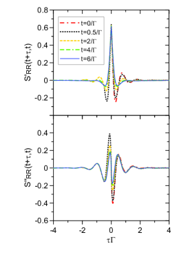
Figure 8: Auto-correlation function $S_{RR}$ in terms of their real and imaginary parts (in units of $e^{2}\Gamma^{2}/\hbar^{2}$) in a single-level nanostructure for different $t$ as a function of $\tau$. Where $\varepsilon=\Gamma$, with $\Gamma_{L}=\Gamma_{R}=0.5\Gamma$, $W_{L}=W_{R}=5\Gamma$, $eV=10\Gamma$, at $k_{B}T=0.5\Gamma$ for both two leads Yang2014 .

Figure 8 plots the auto-correlation function of the right lead for several different $t$. This allows one to monitor the transient processes until the system reaches its steady state, at which these correlations come to only depend on the time difference $\tau$ between the measurements. As one can see, both the real and imaginary parts of correlation functions approach the steady-state values at $t\simeq 5/\Gamma$. The real part of the auto-correlation has a maximal value at $\tau=0$ (namely when it is measured in the same time), this gives the current fluctuation, $\langle I^{2}(t)\rangle-\langle I(t)\rangle^{2}$, and this current fluctuation is independent of the observing time $t$ (less transient). In fact, the current fluctuation, $\langle I^{2}(t)\rangle-\langle I(t)\rangle^{2}$, is mainly contributed from $S^{(3)}$ and $S^{(4)}$ in Eq. (136). From the expression of Eq. (III.1), one can see that $S^{(3)}$ describes the current correlation between an electron tunneling from the dot to the leads at time $t$ and another electron tunneling from the leads to the dot at time $t+\tau$, and $S^{(4)}$ is given by the opposite processes. These processes have the maximum contribution to the current correlation at $\tau=0$. While, $S^{(1)}$ and $S^{(2)}$ describe the correlations of electron tunnelings in the same direction (namely both tunnelings from the leads to the dot or from the dot to the leads), and has a minimum contribution at $\tau=0$, due to the Pauli exclusion principle. When the time difference $\tau$ gets larger, the auto-correlation decays rather faster, and it reaches to zero after $\tau>2/\Gamma$, i.e. the correlation vanishes. With the observing time goes on, the real part of auto-correlation becomes more and more symmetric, and the imaginary part gets more antisymmetric. Eventually they become fully symmetric and antisymmetric functions of $\tau$, respectively, in the steady-state limit, as one expected. It is also found that the cross-correlation is rather small (about of one order of magnitude smaller in comparison with the auto-correlation) that it is not presented in Fig. 8.

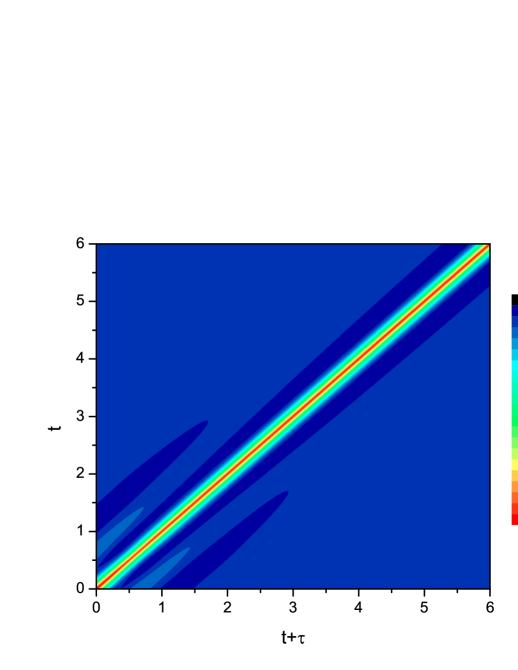
Figure 9: The contour plot of the real part of the total current-current correlation, $S^{\prime}(t+\tau,t)$ (in units of $e^{2}\Gamma^{2}/\hbar^{2}$), in the single-level nanostructure in the two-time plane (scaled by $\Gamma$). Here the parameter $\varepsilon=\Gamma$, with $\Gamma_{L}=\Gamma_{R}=0.5\Gamma$, $W_{L}=W_{R}=5\Gamma$, $eV=10\Gamma$, at $k_{B}T=0.5\Gamma$ for both two leads Yang2014 .

To have a more general picture how the system reaches the steady state, here a contour plot of the real part of the total-correlation in the 2-D time domain is presented in Fig 9. As one can see, it is symmetric in the diagonal line ($\tau=0$), as a consequence of the identity: $S_{\alpha\alpha^{\prime}}(t+\tau,t)=S^{*}_{\alpha^{\prime}\alpha}(t,t+\tau)$. The contour-plot clearly shows an oscillating profile of the correlation in the region $t<3/\Gamma$. The oscillation quickly decays for the time period $3/\Gamma<t<5/\Gamma$. The correlation reaches a steady-state value after $t\simeq 5/\Gamma$. The imaginary part has much the same behavior, except that it has an antisymmetric profile in terms of $t$ and $t+\tau$. This gives the whole picture of the transient current-current correlations.

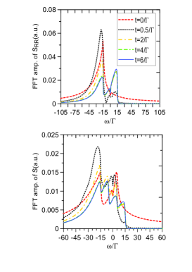
Figure 10: The FFT amplitude of the auto-correlation $S_{RR}$ and the total correlation $S$ in the single-level nanostructure as a function of $\omega$ (in units of $\Gamma$). Where $\varepsilon=5\Gamma$, $\Gamma_{L}=\Gamma_{R}=0.5\Gamma$, $W_{L}=W_{R}=15\Gamma$, $eV=20\Gamma$, $k_{B}T=0.1\Gamma$ for both two leads Yang2014 .

To see the energy structure in electron transports through the transient current-current correlations, one can use the fast Fourier transform (FFT) to convert the correlation functions from the time domain ($\tau$) into the frequency domain for different observing time $t$. The result gives the standard definition of the transient noise spectra. Figure 10 plots the FFT amplitude of the auto-correlation $S_{RR}(t+\tau,t)$ and the total-correlation $S(t+\tau,t)$. From Fig. 10, one can analyze the electron transport properties through the noise spectra not only just in the steady state, but also in the entire transient regime. To make the energy structures manifest in the transient noise spectra, one can let the initial temperature approach zero ($k_{B}T=0.1\Gamma$). The right-lead auto-correlation shows only one single peak at $\omega_{-}=-\omega_{R}=-|\mu_{R}-\varepsilon|$ in the beginning. This is because the dot is initially empty so that electron tunnelings from the Fermi surface of the right lead to the dot have a maximum probability. This peak corresponds to the energy absorption of the electron tunnelings. On the other hand, we also observed that the tunneling process for $\omega>eV$ can happen in the transient regime, which is forbidden in the steady state near zero temperature Rothstein2009 ; Yang2014 . As the time $t$ varies, the second peak shows up. This comes from backward electron tunnelings (i.e. emission processes) from dot to the right lead, with the peak edge locating at the resonance frequency $\omega_{+}=\omega_{R}=|\mu_{R}-\varepsilon|$. Note that with a finite bandwidth spectral density, the spectrum decays when the frequency passes over the resonant frequencies, which is different from the WBL where the spectrum is flat Rothstein2009 ; Yang2014 . The noise spectrum still has a dip at zero frequency in both the transient and steady-state regimes. Furthermore, as one see it needs more time to reach steady state when electrons transit from the leads to the dot, due to the difference of the degrees of freedom between the dot and the leads. Specifically, since there are infinity energy levels in the lead but only one level in the dot system, electrons transiting from the dot to the lead has much smaller probability to return back to the dot, in comparison of the electrons transiting from lead into the dot, as a dissipation effect. Thus, it takes longer time to reach steady state for electrons tunneling from the leads to the central dot. This effect will be reduced if we take a small band width.

The FFT amplitude of the total-correlation has the same properties as the right auto-correlation, with two more peaks coming from the left auto-correlation functions as effects of the emission and absorption processes between the left lead and the central dot. By calculating the individual contribution of the four terms in the auto-correlation expression (Eq. (136)-(136)), it shows that $S^{(3)}$ and $S^{(4)}$ dominate the noise of the current correlations for an electron tunneling from the dot to the lead and another electron tunneling from the lead to the dot. The contributions from $S^{(1)}$ and $S^{(2)}$ are much smaller because they describe the correlations of electron tunnelings in the same direction (namely both tunnelings from the leads to the dot or from the dot to the leads), and mostly contribute to the noise around zero frequency, due to the Pauli exclusion principle.

III.2 Master equation approach to transient quantum transport in nanostructures incorporating initial correlations

Quantum transport incorporating initial correlations in nanostructures is a long-standing problem in mesoscopic physics Haug2008 . In the past two decades, investigations of quantum transport have been mainly focused on steady-state phenomena Datta1995 ; Blanter2000 ; Imry2002 , where initial correlations are not essential due to memory loss. Recent experimental developments allow one to measure transient quantum transport in different nano and quantum devices Lu2003 ; Bylander2005 ; Gustavsson2008 . In the transient transport regime, initial correlations could induce different transport effects. In this section, using the exact master equation approach Tu2008 ; Jin2010 ,one can address the transient quantum transport incorporating initial correlations.

Transient quantum transport was first proposed by Cini Cini1980 , under the so-called partition-free scheme. In this scheme, the whole system (the device system plus the leads together) is in thermal equilibrium up to time $t=0$, and then one applies an external bias to let electrons flow. Thus, the device system and the leads are initially correlated. Stefanucci et. al. Stefanucci2004 ; Stefanucci2007 adopted non-equilibrium Green functions with the Kadanoff-Baym formalism Kadanoff1962 to investigate transient quantum transport with the partition-free scheme. They obtained an analytic transient transport current in the wide-band limit. In these works Stefanucci2004 ; Stefanucci2007 , the transport solution is given in terms of the non-equilibrium Green functions of the total system, rather than the Green functions for the device part in the nanostructures Wingreen1993 .

In fact, earlier investigations of the time-dependent electron transport in solid-state physics had largely used the Kubo formula in the linear response regime Kubo1965 ; Mahan1990 and the semiclassical Boltzmann equation Cer1975 ; Smith1989 . For nanostructural devices, which have an extremely short length scale ($\sim nm$) and an extremely fast time scale ($\sim ps$ to $fs$), the semiclassical Boltzmann equation is most likely inapplicable and the nonlinear response effect must be taken into account Haug2008 . An alternative approach to investigate transient quantum transport is the master equation approach developed particularly for nanostructures Schoeller1994 ; Jin2008 ; Tu2008 ; Jin2010 ; Gurvitz1996 which we have given a complete description in Sec. II.3. However, the exact master equation given in Sec. II.3 is derived in the partitioned scheme in which the system and the leads is initially uncorrelated, the same situation considered in the non-equilibrium Green function technique in Keldysh formalism in Sec. II.2. Realistically, it is possible and often unavoidable in experiments that the device system and the leads are initially correlated. Therefore, the transient transport theory based on the master equation that takes the effect of initial correlations into account becomes necessary.

In this subsection, we present the exact master equation including the effect of initial correlations for non-interacting nanostructures through the extended quantum Langevin equation Yang2015 . It is found that the initial correlations only affect the fluctuation dynamics of the device system, while the dissipation dynamics remains the same as in the case of initially uncorrelated systems. The transient transport current in the presence of initial system-lead and lead-lead correlations is also obtained directly from the exact master equation. Both the partitioned and the partition-free schemes studied in previous works  Wingreen1993 ; Stefanucci2004 ; Stefanucci2007 are naturally reproduced in this theory. Taking an experimentally realizable nano-fabrication system, a single-level quantum dot coupled to two one-dimensional tight-binding leads, as a specific example, the initial correlation effects in the transient transport current as well as in the density matrix of the device system are discussed in details.

Consider a nanostructure consisting of a quantum device coupled with two leads (the source and the drain), described by a Fano-Anderson Hamiltonian (II.3). Because the system and the leads are coupled through electron tunnelings, and the electron-electron interactions in the device are ignored, the total Hamiltonian has a bilinear form of the electron creation and annihilation operators, the master equation describing the time evolution of the reduced density matrix of the device system, $\rho(t)=\rm{Tr}_{E}[\rho_{tot}(t)]$, can have the following general bilinear form Tu2008 ; Tu2012a ; Jin2010 ; Yang2014 as shown in Sec. II.3:

$${d\rho(t)\over dt} =-i\big{[}H^{\prime}_{S}(t),\rho(t)\big{]}+\sum_{ij}\big{\{}\bm{\gamma}_{ij}(t)\big{[}2a_{j}\rho(t)a_{i}^{{\dagger}}$$

$$-a_{i}^{{\dagger}}a_{j}\rho(t)-\rho(t)a_{i}^{{\dagger}}a_{j}\big{]}+\widetilde{\bm{\gamma}}_{ij}(t)\big{[}a_{i}^{{\dagger}}\rho(t)a_{j}$$

$$-a_{j}\rho(t)a_{i}^{{\dagger}}+a_{i}^{{\dagger}}a_{j}\rho(t)-\rho(t)a_{j}a_{i}^{{\dagger}}\big{]}\big{\}}$$

$$= -i\big{[}H_{S}(t),\rho(t)\big{]}+\sum_{\alpha}\big{[}\mathcal{L}^{+}_{\alpha}(t)+\mathcal{L}^{-}_{\alpha}(t)\big{]}\rho(t).$$ (140)

Here the renormalized Hamiltonian $H^{\prime}_{S}(t)=\sum_{ij}\bm{\varepsilon}^{\prime}_{ij}(t)a_{i}^{{\dagger}}a_{j}$, and the coefficient $\bm{\varepsilon}^{\prime}_{ij}(t)$ is the corresponding renormalized energy matrix of the device system, including the energy shift of each level and the lead-induced couplings between different levels. The time-dependent dissipation coefficients $\bm{\gamma}_{ij}(t)$ and the fluctuation coefficients $\widetilde{\bm{\gamma}}_{ij}(t)$ take into account all the back-action effects between the device system and the reservoirs. The current superoperators of lead $\alpha$, $\mathcal{L}^{+}_{\alpha}(t)$ and $\mathcal{L}^{-}_{\alpha}(t)$, determining the transport current from lead $\alpha$ to the device system is given by Eq. (II.3) Jin2010 .

When the device system and the leads are initially correlated, i.e. $\rho_{tot}(t_{0})\neq\rho(t_{0})\otimes\rho_{E}(t_{0})$, it would be challenging to use the Feynman-Vernon influence functional approach to derive the master equation. Alternately, one can use the extended quantum Langevin equation (III.1) to determine the time-dependent coefficients in the master equation when the initial system-lead correlations are presented Yang2015 . Since the quantum Langevin equation is derived exactly from the Heisenberg equation of motion, it is valid for an arbitrary initial state of the device system and the leads.

To determine the time-dependent coefficients in the master equation (III.2), one can compute the equation of motion of the single-particle density matrix of the device system, $\bm{\rho}^{(1)}_{ij}(t)=\langle a_{j}^{\dagger}(t)a_{i}(t)\rangle={\rm Tr}[a_{j}^{\dagger}a_{i}\rho(t)]$ from the master equation (III.2). The result is given by

$$\frac{d}{dt}\bm{\rho}^{(1)}_{ij}(t)= \big{\{}\bm{\rho}^{(1)}(t)\big{[}i\bm{\varepsilon}^{\prime}(t)-\bm{\gamma}(t)\big{]}\big{\}}_{ij}$$

$$-\big{\{}\big{[}i\bm{\varepsilon}^{\prime}(t)+\bm{\gamma}(t)\big{]}\bm{\rho}^{(1)}(t)\big{\}}_{ij}+\widetilde{\bm{\gamma}}_{ij}(t).$$ (141)

It is interesting to see that the homogenous master equation of motion generates an inhomogeneous equation of motion for the single particle density matrix. The inhomogeneous term in Eq. (141) is indeed induced by various initial system-lead and lead-lead correlations, which will be shown next.

On the other hand, Eq. (141) can also be derived from the exact solution of the quantum Langevin equation, Eq. (132). Explicitly, the single-particle correlation function of the device system calculated from the solution of Eq. (132) is given by

$$\bm{\rho}^{(1)}_{ij}(\tau,t) =\langle a^{\dagger}_{j}(t)a_{i}(\tau)\rangle$$

$$=\big{[}\bm{u}(\tau,t_{0})\bm{\rho}^{(1)}(t_{0})\bm{u}^{{\dagger}}(t,t_{0})+\bm{v}(\tau,t)\big{]}_{ij},$$ (142)

which indeed has exactly the same form as Eq. (115) for the initially partitioned state, and

$$\bm{v}_{ij}(\tau,t)\!= \!\sum_{\alpha}\!\!\int_{t_{0}}^{\tau}\!\!d\tau_{1}\!\!\int_{t_{0}}^{t}\!\!\!d\tau_{2}[\bm{u}(\tau,\tau_{1})\widetilde{\bm{g}}_{\alpha}(\tau_{1},\tau_{2})\bm{u}^{{\dagger}}(t,\tau_{2})]_{ij},$$ (143)

which also has the same form as Eq. (116), but the time non-local integral kernel, $\widetilde{\bm{g}}_{\alpha}(\tau,\tau^{\prime})$ of Eq. (104b), is now modified by the additional initial system-lead correlations as

$$\widetilde{\bm{g}}_{\alpha ij}(\tau,\tau^{\prime})=\widetilde{\bm{g}}^{se}_{\alpha ij}(\tau,\tau^{\prime})+\widetilde{\bm{g}}^{ee}_{\alpha ij}(\tau,\tau^{\prime}),$$ (144)

where

$$\widetilde{\bm{g}}^{se}_{\alpha ij}(\tau,\tau^{\prime})= -2i\sum_{k}\!\!\Big{[}V_{i\alpha k}(\tau)e^{-i\int_{t_{0}}^{\tau}\epsilon_{\alpha k}(\tau_{1})d\tau_{1}}\langle a_{j}^{\dagger}(t_{0})c_{\alpha k}(t_{0})\rangle\delta(\tau^{\prime}-t_{0})$$

$$~{}~{}~{}~{}~{}~{}~{}~{}~{}~{}~{}~{}~{}-V^{*}_{j\alpha k}(\tau^{\prime})e^{i\int_{t_{0}}^{\tau^{\prime}}\epsilon_{\alpha k}(\tau_{1})d\tau_{1}}\langle c^{\dagger}_{\alpha k}(t_{0})a_{i}(t_{0})\rangle\delta(\tau-t_{0})\Big{]},$$ (145a)

$$\widetilde{\bm{g}}^{ee}_{\alpha ij}(\tau,\tau^{\prime})= \sum_{\alpha^{\prime}}\sum_{kk^{\prime}}V_{i\alpha k}(\tau)e^{-i\int_{t_{0}}^{\tau}\epsilon_{\alpha k}(\tau_{1})d\tau_{1}}V^{*}_{j\alpha^{\prime}k^{\prime}}(\tau^{\prime})e^{i\int_{t_{0}}^{\tau^{\prime}}\epsilon_{\alpha^{\prime}k^{\prime}}(\tau_{1})d\tau_{1}}\langle c_{\alpha^{\prime}k^{\prime}}^{\dagger}(t_{0})c_{\alpha k}(t_{0})\rangle.$$ (145b)

As one can see, $\widetilde{\bm{g}}^{se}_{\alpha}(\tau,\tau^{\prime})$ is proportional to all the initial electron correlations between the system and the leads, and $\widetilde{\bm{g}}^{ee}_{\alpha}(\tau,\tau^{\prime})$ is associated with the initial electron correlations in the leads. Physically, the electron correlation Green function $\bm{v}(\tau,t)$ characterizes all possible electron fluctuation processes due to the initial system-lead correlations and initial lead-lead correlations, both are induced by the inhomogeneity of the quantum Langevin equation (III.1). Also, Eq. (142) indeed gives the exact solution of the lesser Green function incorporating initial correlations. Thus, through the extended quantum Langevin equation, we obtain the most general solution for the single-particle correlation function $\bm{\rho}^{(1)}(\tau,t)$ (the lesser Green function) and the electron correlation Green function $\bm{v}(\tau,t)$ in the Keldysh nonequilibrium Green function technique.

With the above general solution Eq. (142), it is found that

$$\frac{d}{dt}\bm{\rho}_{ij}^{(1)}(t)\!=\![\dot{\bm{u}}(t,t_{0})\bm{u}^{-1}(t,t_{0})\bm{\rho}^{(1)}(t)+{\rm H.c.}]_{ij}$$

$$~{}~{}~{}~{}~{}~{}~{}~{}~{}~{}~{}~{}~{}~{}-\![\dot{\bm{u}}(t,t_{0})\bm{u}^{-1}\!(t,t_{0})\bm{v}(t,t)\!+\!{\rm H.c.}]_{ij}\!+\!\frac{d}{dt}\bm{v}_{ij}(t,t).$$ (146)

The last two terms in the above equation are inhomogeneous and proportional to the electron correlation Green function $\bm{v}(\tau,t)$ and, therefore, are purely induced by various initial system-lead and lead-lead correlations through the integral kernel $\widetilde{\bm{g}}_{\alpha}(\tau,\tau^{\prime})$. Now, by comparing Eq. (141) with Eq. (146), the time-dependent renormalized energy $\bm{\varepsilon}^{\prime}_{ij}(t)$, dissipation, and fluctuation coefficients $\bm{\gamma}_{ij}(t)$ and $\widetilde{\bm{\gamma}}_{ij}(t)$ in the master equation incorporating initial correlations are uniquely determined as follows,

$$\bm{\varepsilon}^{\prime}_{ij}(t) =\frac{i}{2}\big{[}\dot{\bm{u}}(t,t_{0})\bm{u}^{-1}(t,t_{0})-{\rm H.c.}\big{]}_{ij}$$

$$=\bm{\varepsilon}_{ij}(t)-\frac{i}{2}\sum_{\alpha}[\bm{\kappa}_{\alpha}(t)-\bm{\kappa}^{\dagger}_{\alpha}(t)]_{ij},$$

$$\bm{\gamma}_{ij}(t) =-\frac{1}{2}\big{[}\dot{\bm{u}}(t,t_{0})\bm{u}^{-1}(t,t_{0})+{\rm H.c.}\big{]}_{ij}$$

$$=\frac{1}{2}\sum_{\alpha}[\bm{\kappa}_{\alpha}(t)+\bm{\kappa}^{\dagger}_{\alpha}(t)]_{ij},$$

$$\widetilde{\bm{\gamma}}_{ij}(t) =\frac{d}{dt}\bm{v}_{ij}(t,t)-[\dot{\bm{u}}(t,t_{0})\bm{u}^{-1}(t,t_{0})\bm{v}(t,t)+\rm H.c.]_{ij}$$

$$=-\sum_{\alpha}[\bm{\lambda}_{\alpha}(t)+\bm{\lambda}^{\dagger}_{\alpha}(t)]_{ij}.$$

From the above results, one can see that the renormalized energy $\bm{\varepsilon}^{\prime}_{ij}(t)$ and the dissipation coefficients $\bm{\gamma}_{ij}(t)$ are independent of the initial correlations and are identical to the results given in Eqs. (111a) and (111b) for the decoupled initial state. The fluctuation coefficients $\widetilde{\bm{\gamma}}_{ij}(t)$ also have the same form of Eq. (111c) as for the initially partitioned state, but the electron correlation Green function $\bm{v}(t,t)$ takes into account both the initial system-lead and the initial lead-lead correlations through Eqs. (144-145). In other words, initial correlations only contribute to the fluctuation-related dynamics of the device system, and the expressions of all the time-dependent coefficients in the master equation (III.2) remain the same. Correspondingly, the current superoperators in the master equation (III.2) incorporating initial system-lead correlations, $\mathcal{L}^{+}_{\alpha}(t)$ and $\mathcal{L}^{-}_{\alpha}(t)$, are still given by the same form of Eq. (112) as in the initially partitioned state. As a result, the transient transport current $I_{\alpha}(t)$ incorporating with the initial system-lead correlations is still given by the same equation (II.3)

$$I_{\alpha}(t)\!=\!-2e{\rm Re}\!\!\int_{t_{0}}^{t}\!\!d\tau{\rm Tr} [\bm{g}_{\alpha}(t,\tau)\!\bm{\rho}^{(1)}(\tau,t)\!-\!\widetilde{\bm{g}}_{\alpha}(t,\tau)\bm{u}^{{\dagger}}(t,\tau)].$$ (148)

Thus, the transient quantum transport incorporating initial correlations is fully expressed in terms of the standard non-equilibrium Green functions of the device system. The initially uncorrelated case (the partitioned scheme) in Sec. II.3 is a special case in which the initial system-lead correlations vanish so that $\widetilde{\bm{g}}^{se}_{\alpha}(t,\tau)=0$, and then the time non-local integral kernel $\widetilde{\bm{g}}_{\alpha}(t,\tau)$ is simply reduced to Eq. (104b).

In conclusion, the exact master equation (III.2) describes the non-Markovian dynamics and transient quantum transport of nano-device systems coupled to leads involving various initial system-lead and lead-lead correlations. In fact, the exact master equation with or without the initial system-lead correlations is given by the same formula, except for the time non-local integral kernel $\widetilde{\bm{g}}_{\alpha}(t,\tau)$, which is determined by Eq. (104b) for the initially uncorrelated states between the system and the leads, but it must be modified by Eqs. (144-145) for the initially correlated states.

In the literature Breuer2002 , it is claimed that in the master equation formally derived through the Nakajima-Zwanzig (NZ) operator projective technique Nakajima1958 ; Zwanzig1960 , the initial system-lead correlations would induce an inhomogeneous term in the master equation. However, the so-called inhomogeneous term in the NZ master equation is a misunderstanding in Breuer2002 . In a recent work Yang2016 , we show explicitly that the so-called initial system-lead correlations induced inhomogeneous term in the NZ master equation is indeed a homogeneous term both in terms of projected Hilbert subspaces in the original NZ master equation formalism and in the master equation in terms of the reduced density matrix after taking trace over the environment states. The result must be similar to Eq. (III.2) for Fano-Anderson model where the initial system-lead correlations are embedded in the fluctuation coefficients, as given explicitly in this section.

It should be pointed out that if the leads are made by superconductors, there may be initial pairing correlations. Then, the master equation (III.2) may need to be modified. Further investigation of this problem is in progress Lai . Nevertheless, the master equation (III.2) is sufficient for the description of transient quantum transport in nanostructures with the initial correlations given in Eq. (145). In fact, because the total Hamiltonian has a bilinear form of the electron creation and annihilation operators, [see Eq. (II.3)], all other correlation functions can be fully determined by the two basic nonequilibrium Green’s functions, $\bm{u}(t,t_{0})$ and $\bm{v}(\tau,t)$. The non-Markovain memory effects, including the initial-state dependence, which are fully embedded in the time-dependent dissipation and fluctuation coefficients in the exact master equation (III.2), are consistently determined by these two basic nonequilibrium Green functions.

Figure 11: A schematic plot of a single-level quantum dot coupled to two one-dimensional tight-binding leads

To be specific, we consider an experimentally realizable nano-fabrication system, a single-level quantum dot coupled to the source and the drain, which are modeled by two one-dimensional tight-binding leads (see Fig. 11). The Hamiltonian of the whole system is given by

$$H(t)= \,\,\varepsilon_{c}a^{\dagger}a-\sum_{\alpha}(\lambda_{\alpha 1}a^{{\dagger}}c_{\alpha 1}+\lambda^{*}_{\alpha 1}c_{\alpha 1}^{{\dagger}}a)$$

$$+\sum_{\alpha}\sum_{n=1}^{\mathcal{N}}[\epsilon_{\alpha}+U_{\alpha}(t)]c_{\alpha n}^{\dagger}c_{\alpha n}$$

$$-\sum_{\alpha}\sum_{n=1}^{\mathcal{N}-1}(\lambda_{\alpha}c_{\alpha n}^{{\dagger}}c_{\alpha n+1}+\lambda^{*}_{\alpha}c_{\alpha n+1}^{{\dagger}}c_{\alpha n}),$$ (149)

where $a$ ($a^{\dagger}$) is the annihilation (creation) operator of the single-level dot with the energy level $\varepsilon_{c}$, and $c_{\alpha n}$ ($c_{\alpha n}^{\dagger}$) the annihilation (creation) operator of lead $\alpha$ at site $n$. All the sites in lead $\alpha$ have an equal on-site energy $\epsilon_{\alpha}$. $U_{\alpha}(t)$ is the time-dependent bias voltage applied on lead $\alpha$ to shift the on-site energy. The second term in Eq. (149) describes the coupling between the quantum dot and the first site of the lead $\alpha$ with the coupling strength $\lambda_{\alpha 1}$. The last term characterizes the electron tunneling between two consecutive sites in lead $\alpha$ with tunneling amplitude $\lambda_{\alpha}$, and $\mathcal{N}$ is the total number of sites on each lead.

In the $k$-space, the Hamiltonian (149) becomes

$$H(t)= \varepsilon_{c}a^{\dagger}a+\sum_{\alpha k}\epsilon_{\alpha k}(t)c_{\alpha k}^{\dagger}c_{\alpha k}$$

$$+\sum_{\alpha k}[V_{\alpha k}a^{{\dagger}}c_{\alpha k}+V^{*}_{\alpha k}c^{{\dagger}}_{\alpha k}a],$$ (150)

where $\epsilon_{\alpha k}(t)=\epsilon_{\alpha k}+U_{\alpha}(t)$, $\epsilon_{\alpha k}=\epsilon_{\alpha}-2|\lambda_{\alpha}|\cos k$, and $V_{\alpha k}=-\sqrt{\frac{2}{\mathcal{N}}}\lambda_{\alpha 1}e^{-i\phi}\sin k$. Hamiltonian (150) has the same structure as Hamiltonian (II.3). The time non-local integral kernel $g_{\alpha}(t,\tau)$ is given by

$$g_{\alpha}(\tau,\tau^{\prime})=\sum_{k}|V_{\alpha k}|^{2}e^{-i\int^{\tau}_{\tau^{\prime}}\epsilon_{\alpha k}(\tau_{1})d\tau_{1}}.$$ (151)

Because both the left and the right leads are modeled by the same tight-binding model, namely, $\epsilon_{L}=\epsilon_{R}=\epsilon_{0}$ and $\lambda_{L}=\lambda_{R}=\lambda_{0}$. When the site number $\mathcal{N}\rightarrow\infty$, without applying bias [$U_{\alpha}(t)=0$], the general solution of the Green function $u(t,t_{0})$ is Zhang2012 ,

$$u(t,t_{0})=\int\frac{d\epsilon}{2\pi}{\cal D}(\epsilon)e^{-i\epsilon(t-t_{0})},$$ (152)

with

$${\cal D}(\epsilon)= 2\pi\sum_{j\pm}Z_{j}\delta(\epsilon-\epsilon_{j})\Theta(\eta^{2}-\eta^{2}_{\pm})$$

$$+\frac{\Gamma(\epsilon)}{\left[\epsilon-\varepsilon_{c}-\eta^{2}(\epsilon-\epsilon_{0})/2\right]^{2}+\Gamma^{2}(\epsilon)/4},$$ (153)

where $\eta^{2}=\eta^{2}_{L}+\eta^{2}_{R}$ and $\eta_{\alpha}$ is the coupling ratio $|\lambda_{\alpha 1}|/|\lambda_{0}|$ of lead $\alpha$. The spectral density $\Gamma(\epsilon)=\Gamma_{L}(\epsilon)+\Gamma_{R}(\epsilon)$ with

$$\Gamma_{\alpha}(\epsilon) =\left\{\begin{array}[]{ll}\eta^{2}_{\alpha}\sqrt{4|\lambda_{0}|^{2}-(\epsilon-\epsilon_{0})^{2}}&\mbox{if }|\epsilon-\epsilon_{0}|\leq 2|\lambda_{0}|,\\ \\ 0&\mbox{otherwise .}\end{array}\right.$$ (157)

In the solution (153), the first term characterizes the localized state Mahan1990 with energy $\epsilon_{j}$ lying outside the energy band when the total coupling ratio $\eta^{2}\geq\eta^{2}_{\pm}$, where $\eta^{2}_{\pm}=2\mp\frac{\Delta}{|\lambda_{0}|}$ is the critical coupling ratio. Localized states are also referred to as dressed bound states. Since the energy bands of the two leads overlap, there are at most two localized states. The amplitude and the frequency of the localized state are given by Yin

$$Z_{\pm} =\frac{1}{2}\frac{(\eta^{2}-2)\sqrt{4(\eta^{2}-1)|\lambda_{0}|^{2}+\Delta^{2}}\pm\eta^{2}\Delta}{(\eta^{2}-1)\sqrt{4(\eta^{2}-1)|\lambda_{0}|^{2}+\Delta^{2}}},$$ (158a)

$$\epsilon_{\pm} =\epsilon_{0}+\frac{(\eta^{2}-2)\Delta}{2(\eta^{2}-1)}\pm\frac{\eta^{2}\sqrt{4(\eta^{2}-1)|\lambda_{0}|^{2}+\Delta^{2}}}{2(\eta^{2}-1)},$$ (158b)

where $\Delta=\varepsilon_{c}-\epsilon_{0}$. When a finite bias is applied, the above result should be modified accordingly, see Fig. 12, and the discussion given over there.

As a result, the effect of initial correlations will be maintained in the steady-state limit through the localized states, the first term in the solution of Eq. (153). This manifests a long-time non-Markovian memory effect. The second term in Eq. (153) is the contribution from the continuous energy spectra, which causes electron dissipation (damping) in the dot system. Once the solution of $u(t,t_{0})$ is given, the electron correlation Green function $v(\tau,t)$ can be easily calculated with the following general relation:

$$v(\tau,t)=\sum_{\alpha}\int_{0}^{\tau}d\tau_{1}\int_{0}^{t}d\tau_{2}u(\tau,\tau_{1})\widetilde{g}_{\alpha}(\tau_{1},\tau_{2})u^{*}(t,\tau_{2}).$$ (159)

Thus, by solving the Green function $u(t,t_{0})$ and the correlation Green function $v(\tau,t)$, the density matrix and the transient transport current can be fully determined,

$$\rho^{(1)}(t)=|u(t,t_{0})|^{2}\rho^{(1)}(t_{0})+v(t,t)=n(t),$$ (160a)

$$I_{\alpha}(t)=-2e{\rm Re}\!\!\int_{t_{0}}^{t}\!\!d\tau[g_{\alpha}(t,\tau)\rho^{(1)}(\tau,t)-\widetilde{g}_{\alpha}(t,\tau)u^{*}(t,\tau)].$$ (160b)

Consider two different initial states as examples. One is the partition-free scheme, in which the whole system is in equilibrium before the external bias is switched on. The other is the partitioned scheme in which the initial state of the dot system is uncorrelated with the leads before the tunneling couplings are turned on, the dot can be in any arbitrary initial state $\rho(t_{0})$ and the leads are initially at separated equilibrium state. Both of these schemes can be realized through different experimental setups. By comparing the transient transport dynamics for these two initial schemes, one will see in what circumstances the initial correlations will affect quantum transport in the transient regime as well as in the steady-state limit.

In the partition-free scheme, the whole system is in equilibrium before the external bias voltage $U_{\alpha}(t)$ is switched on. The applied bias voltage is set to be uniform on each lead such that $U_{\alpha}(t)=U_{\alpha}\Theta(t-t_{0})$, so $H(t\leq t_{0})\equiv H$ is time-independent. The initial density matrix of the whole system is given by $\rho_{tot}(t_{0})=\frac{1}{Z}e^{-\beta(H-\mu N)}$, where $H$ and $N$ are respectively the total Hamiltonian and the total particle number operator at initial time $t_{0}$. The whole system is initially at the temperature $\beta=1/k_{B}T$ with the chemical potential $\mu$. When $t>t_{0}$, a uniform bias voltage is applied to each lead, the whole system then suddenly change into a non-equilibrium state. In this case, the calculations of initial correlations, $\langle a^{\dagger}(t_{0})c_{\alpha k}(t_{0})\rangle$ and $\langle c^{\dagger}_{\alpha^{\prime}k^{\prime}}(t_{0})c_{\alpha k}(t_{0})\rangle$, and the corresponding time non-local integral kernel, $\widetilde{g}_{\alpha}(\tau,\tau^{\prime})=\widetilde{g}^{se}_{\alpha}(\tau,\tau^{\prime})+\widetilde{g}^{ee}_{\alpha}(\tau,\tau^{\prime})$, are very complicated, see the detailed calculations given in Appendix B of Ref. Yang2015 .

For the partitioned scheme, the dot and the leads are initially uncorrelated, and the leads are initially in equilibrium state $\rho_{E}(t_{0})=\frac{1}{Z}e^{-\sum_{\alpha}\beta_{\alpha}(H_{\alpha}-\mu_{\alpha}N_{\alpha})}$. After $t_{0}$ one can turn on the tunneling couplings between the dot and the leads to let the system evolve Giblin2012 . In comparison with the partition-free scheme, each energy level in lead $\alpha$ shifts by $U_{\alpha}$ to preserve the charge neutrality, i.e., $\epsilon_{\alpha k}\rightarrow\epsilon_{\alpha k}+U_{\alpha}$. Also, $\beta_{L}=\beta_{R}=\beta$ is taken Stefanucci2004 . The initial-state differences between the partition-free and the partitioned schemes can be demonstrated simply in an initial empty dot in the partitioned scheme. In this case, the non-local time system-lead correlation function vanishes, $\widetilde{g}^{se}_{\alpha}(\tau,\tau^{\prime})=0$; the only non-vanishing initial correlation for the partitioned scheme is given by the initial Fermi distribution of the leads: $\langle c^{\dagger}_{\alpha^{\prime}k^{\prime}}(t_{0})c_{\alpha k}(t_{0})\rangle=\delta_{\alpha k,\alpha^{\prime}k^{\prime}}f_{\alpha}(\epsilon_{\alpha k})$, which leads to the time non-local integral kernel $\widetilde{g}_{\alpha}(\tau,\tau^{\prime})=\!\!\int\!\!\frac{d\epsilon}{2\pi}\Gamma_{\alpha}(\epsilon)f_{\alpha}(\epsilon+U_{\alpha})e^{-i(\epsilon+U_{\alpha})(\tau-\tau^{\prime})}$.

The dissipation and localized state dynamics of the electron in the dot system, given by the time evolution of the Green function $u(t,t_{0})$ is shown in Fig. 12. The dissipation dynamics is independent of the initial correlations, so the results of $|u(t)|\equiv|u(t,t_{0}=0)|$ shown in Fig. 12 are the same for both the partition-free and the partitioned schemes. Without applying a bias, in the weak coupling regime: $\eta^{2}=\eta^{2}_{L}+\eta^{2}_{R}<2-\frac{\Delta}{|\lambda_{0}|}$, no localized state occurs so the propagating Green function monotonically decays to zero. In the intermediate coupling regime: $2-\frac{\Delta}{|\lambda_{0}|}\leq\eta^{2}<2+\frac{\Delta}{|\lambda_{0}|}$, one localized state occurs [see the detailed discussion following Eq. (153)]. Correspondingly, $|u(t)|$ decays very fast in the beginning and then gradually approaches to a non-zero constant value in the steady-state limit, as shown in Fig. 12(b). This non-zero steady-state value is the contribution of the localized state. In the strong coupling regime: $\eta^{2}\geq 2+\frac{\Delta}{|\lambda_{0}|}$, two localized states occur simultaneously. One can find that $|u(t)|$ will oscillate in time forever. The oscillation frequency is the energy difference between the two localized states energies, as shown in Fig. 12(c).

When a finite bias is applied, $|u(t)|$ decays slowely in comparison with the unbiased case in the weak coupling regime, where no localized state occurs. In the intermediate coupling regime, it is different from the unbiased case that $|u(t)|$ continuously decays and eventually approaches to zero, see the dashed curve in Fig. 12(b). This implies that the localized state is suppressed by the applied bias. This suppression comes from the fact that the localized states always lie in the band gaps not far away from the band edges Lo2015 . The applied bias enlarges the band energy regime, which could exclude the occurrence of the localized state when the dot-lead coupling strength is not strong enough. The localized state will reappear if one increases the coupling strength. Therefore, in the strong coupling regime, the dissipation dynamics is changed accordingly, in comparison with the unbiased case, where one of the two localized states is suppressed by the applied bias, as shown in Fig. 12(c). As a result, the long-time oscillation behavior seen in the unbiased case does not occur. Only in the very strong coupling regime, the long-time oscillation induced by two localized states could happen, but this may go beyond the physically feasible regime that we are interested in. In summary, for the same dot-lead coupling strength, the applied bias suppresses the effect of one localized state. As a result, $|u(t)|$ still decays to zero in the intermediate coupling regime, and eventually approaches to a constant value in the strong coupling regime.

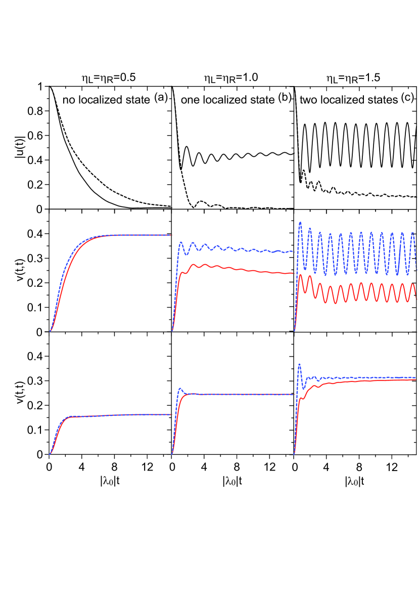
Figure 12: The absolute value of time-dependent propagating Green function $|u(t)|$ and the electron correlation Green function $v(t,t)$ at different coupling ratios (a) $\eta_{L}=\eta_{R}=0.5$, (b) $\eta_{L}=\eta_{R}=1.0$, (c) $\eta_{L}=\eta_{R}=1.5$ with zero bias $eV_{SD}=\mu_{L}-\mu_{R}=U_{L}-U_{R}=0$ and a finite bias $eV_{SD}=\mu_{L}-\mu_{R}=U_{L}-U_{R}=3|\lambda_{0}|$. The energy level of the quantum dot $\varepsilon_{c}=3|\lambda_{0}|$, the band center of the two leads $\epsilon_{0}=2.5|\lambda_{0}|$, and $k_{B}T_{L}=k_{B}T_{R}=3|\lambda_{0}|=k_{B}T$. For the unbiased case, $\mu_{L}=\mu_{R}=2.5|\lambda_{0}|$, and $U_{L}=U_{R}=1.5|\lambda_{0}|$. For the biased case, $\mu_{L}=4|\lambda_{0}|$, $\mu_{R}=|\lambda_{0}|$, $U_{L}=3|\lambda_{0}|$, and $U_{R}=0$. In the graph of $|u(t)|$, solid curves denote the unbiased case, and dash curves denote the biased case. The value $v(t,t)$ in partition-free (blue dash line) and partitioned (red solid line) schemes for the unbiased (the second row) and biased (the third row) cases is presented Yang2015 .

The above different dissipation dynamics with or without a finite bias will significantly affect the electron correlation Green function $v(t,t)$ which characterizes all the system-lead and lead-lead initial correlation effects through the time non-local integral kernel $\widetilde{g}_{\alpha}(\tau,\tau^{\prime})$, see Eqs. (144-145). The numerical results are shown in the second row (without bias) and the third row (with a finite bias) in Fig. 12. In the weak-coupling regime $\eta^{2}<2-\frac{\Delta}{|\lambda_{0}|}$, as we can see that in both the unbiased or biased cases, electron correlation Green function $v(t,t)$ are not significantly different for different initial states. In particular, $v(t,t)$ becomes independent of initial states in the steady state limit. In the intermediate coupling regime $2-\frac{\Delta}{|\lambda_{0}|}\leq\eta^{2}<2+\frac{\Delta}{|\lambda_{0}|}$, $v(t,t)$ is quite different for the partitioned and partition-free schemes in the transient regime, and also approach to different steady-state values for the unbiased case. This shows that the initial correlation effects can be manifested though the localized state in the dot. However, when a finite bias is applied, this significant initial correlation effect disappears. This is because a finite bias suppresses the effect of the localized state, as discussed in the solution of $u(t,t_{0})$. In the strong coupling regime, $\eta^{2}\geq 2+\frac{\Delta}{|\lambda_{0}|}$, the initial correlations effects are more significant. For zero bias, the two localized states generate a strong oscillation in the steady-state solution of $v(t,t)$. The oscillating frequency is just the energy difference of the two localized states. When a bias is applied, one localized state is suppressed so that the oscillation cannot occur in the steady state, as shown in Fig. 12.

Figure 13 shows the electron occupation in the dot and the transient transport current $I_{L}(t)=I_{R}(t)$ in the unbiased case for the partitioned and partition-free schemes. The partition-free system is initially at equilibrium so that the dot contains electrons, while the dot is initially empty in the partitioned scheme. One can see that the effect of the initial correlations vanish in the steady-state limit when the coupling ratio $\eta^{2}<2-\frac{\Delta}{|\lambda_{0}|}$, where the dot does not have localized state. This is because after $u(t,t_{0})$ decays to zero, the steady-state electron occupation is purely determined by $v(t,t)$, which is the same for the partition-free and partitioned schemes, as shown in Fig. 12. This is an evidence of the dot system reaching equilibrium with the leads so that the steady-state electron occupation inside the dot must be independent of the initial states.

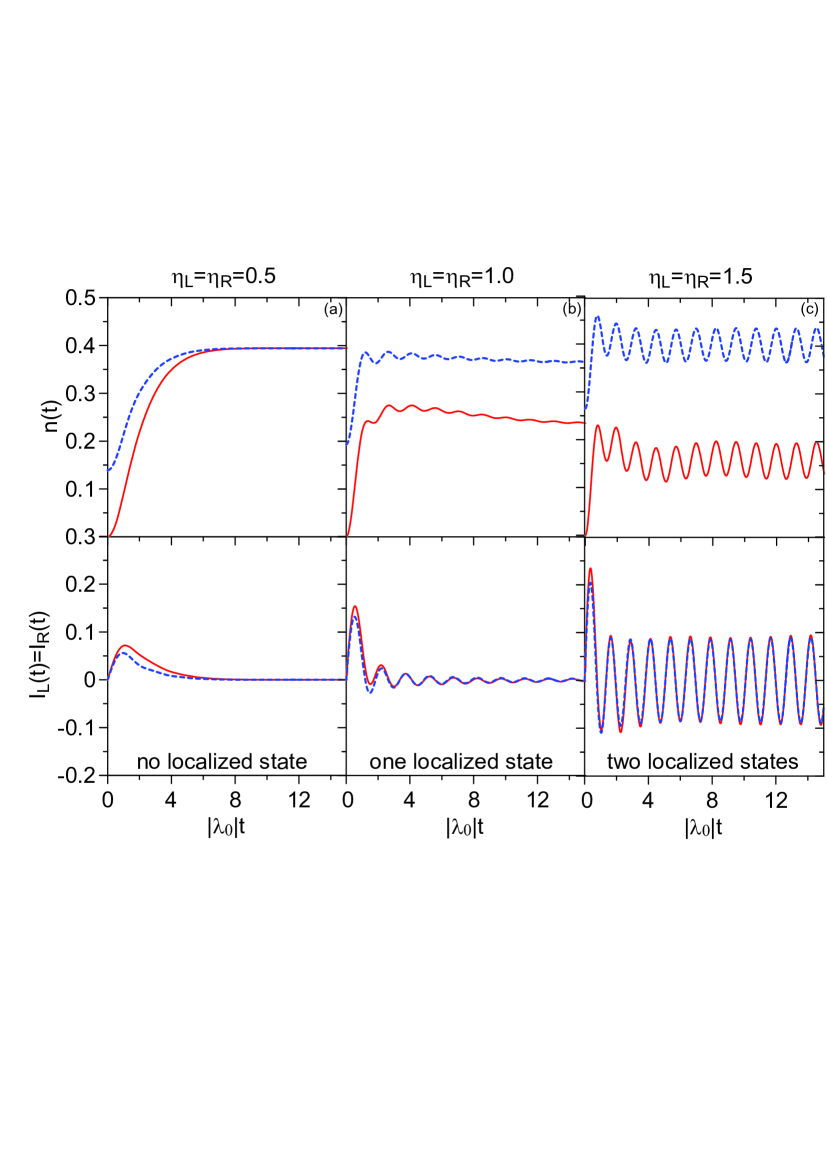
Figure 13: The transient electron occupation of the dot and the transient transport current for the unbiased case at different coupling ratios (a) $\eta_{L}=\eta_{R}=0.5$, (b) $\eta_{L}=\eta_{R}=1.0$, (c) $\eta_{L}=\eta_{R}=1.5$ for the partition-free (blue-dash line) and partitioned (red solid line) schemes. The energy level of the quantum dot $\varepsilon_{c}=3|\lambda_{0}|$, the band center of the two leads $\epsilon_{0}=2.5|\lambda_{0}|$. For the partitioned scheme the leads are prepared at $\mu_{L}=\mu_{R}=2.5|\lambda_{0}|$, and $k_{B}T_{L}=k_{B}T_{R}=3|\lambda_{0}|$. For the partition-free scheme, the system is initially at equilibrium with $\mu=|\lambda_{0}|$ and $k_{B}T=3|\lambda_{0}|$. The applied bias voltage $U_{L}=U_{R}=1.5|\lambda_{0}|$ after $t_{0}=0$ Yang2015 .

However, in the coupling regime $2-\frac{\Delta}{|\lambda_{0}|}\leq\eta^{2}<2+\frac{\Delta}{|\lambda_{0}|}$, the localized state play a significant role in manifesting the initial correlation effects. The different electron occupation in the dot for the partitioned and partition-free schemes is very similar to the behavior of $v(t,t)$, see Fig. 12 and Fig. 13, except for a slightly difference due to the initial occupation, caused by the first term in Eq. (160). Thus, the electron occupation in the dot depends significantly on initial states. Physically, this result implies the breakdown of the equilibrium hypothesis of statistical mechanics, namely after reached the steady state, the system does not approach equilibrium with its environment, and the particle distribution depends on the initial states. This result with localized states agrees indeed with the fact Anderson pointed out in Anderson localization Anderson1958 , namely, the system cannot approach equilibrium when localization occurs. In the strong coupling regime, $\eta^{2}\geq 2+\frac{\Delta}{|\lambda_{0}|}$, two localized states occur, which generates a strong oscillation in the density matrix with the oscillating frequency being the energy difference of the two localized states. This oscillation is maintained in the steady state, where the initial-state dependence becomes more significant, as shown in Fig. 13(c).

The corresponding transient transport current for the partitioned and partition-free schemes approaches to the same value in a every short time scale regardless whether the localized states exist or not. This is because at zero bias, the steady-state transport average current must approach to zero. The transport current will oscillate slightly around the zero value in Fig. 13(b) because one localized state occurs which causes the oscillation of electrons in the dot in the transient regime. When two localized states occur, electrons in the dot oscillate between the two localized states, so that the corresponding transport current follows the same oscillation. In the meantime, the initial-correlation dependence in the transport current is not as significant as in the electron occupation in both the transient regime and the steady-state limit. In fact, the initial correlation effects even can be ignored for the transport current in the steady-state limit, as shown in Fig. 13. The current only oscillates around zero value because of the zero bias.

The time evolution of the electron occupation in the dot and the transient transport current for both the partitioned and the partition-free schemes for the biased case are shown in Fig. 14. Compare Fig. 13 with Fig. 14, one can find that the applied bias restrains most of the oscillation behavior in the electron occupation as well as in the transport current, except for the very beginning of the transient regime. Also, regardless of the existence of localized states, the electron occupation in the dot and also the transport current all approach to steady-state values other than zero due to the non-zero bias. In other words, the localized state has a less effect on the electron occupation and the transport current when a bias is applied. This is because the applied bias suppresses one of the localized states. However, the remaining localized state will result in a slightly different steady-state values for partition-free and partitioned schemes for the electron occupation in the dot. The corresponding transient current flow through the left and right leads are quite different for these two schemes when a bias voltage is applied. In particular, the transient transport current in the right lead is positive in the beginning for the partitioned scheme because the dot is initially empty, and it approaches to a negative steady-state value in both schemes. But the steady-state current is almost independent of the initial correlations as shown in the inset graphs in Fig. 14. These results show that the initial correlation effects have a significant effects in the transient regime for both the electron occupation in the dot and the transport currents between the dot and the leads when a finite bias is applied. In the steady-state limit, it is expected that the initial correlation effects are less important in electron transport currents in comparison with the electron occupation in the dot.

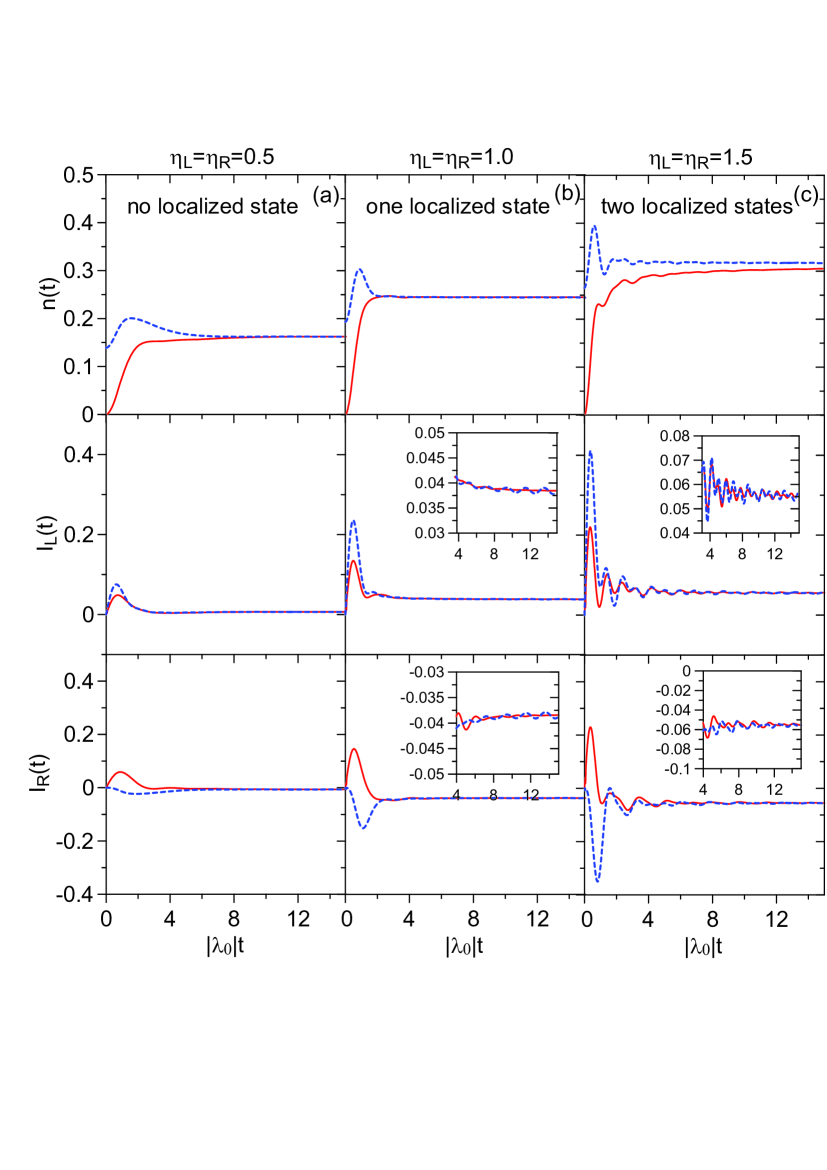
Figure 14: The transient electron occupation of the dot and the transient transport current for the biased case at different coupling ratios (a) $\eta_{L}=\eta_{R}=0.5$, (b) $\eta_{L}=\eta_{R}=1.0$, (c) $\eta_{L}=\eta_{R}=1.5$ for the partition-free (blue-dash line) and partitioned (red solid line) schemes. The energy level of the quantum dot $\varepsilon_{c}=3|\lambda_{0}|$, the band center of the two leads $\epsilon_{0}=2.5|\lambda_{0}|$. For the partitioned scheme the leads are prepared at $\mu_{L}=4|\lambda_{0}|$, $\mu_{R}=|\lambda_{0}|$, and $k_{B}T_{L}=k_{B}T_{R}=3|\lambda_{0}|$. For the partition-free scheme, the system is initially at equilibrium with $\mu=|\lambda_{0}|$ and $k_{B}T=3|\lambda_{0}|$. The applied bias voltage $U_{L}=3|\lambda_{0}|$ and $U_{R}=0$ after $t_{0}=0$ Yang2015 .

In fact, the quantum transport in the presence of localized states was previously studied boundstate1 ; boundstate2 ; boundstate3 ; Dhar2006 ; Stefanucci2007 . In particular, Dhar and Sen considered a wire connected to reservoirs that is modeled by a tight-binding noninteracting Hamiltonian in the partitioned scheme Dhar2006 , and they gave the steady-state solution of the density matrix and the current. Their results show that the memory effects induced by the localized states can be observed such that the density matrix of the system is initial-state dependent. Stefanucci used the Kadanoff-Baym formalism to formally study the localized state effects in the quantum transport in the partition-free scheme Stefanucci2007 . He found that the biased system with localized states does not evolve toward a stationary state. The results here using the master equation approach agree with these results obtained in Refs. Stefanucci2007 and Dhar2006 . The initial-state dependance of the density matrix in the partitioned scheme is indeed obvious in the master equation formalism, as given in Eq. (160). In fact, all these results with the existence of the localized states are fully determined by the solution of the nonequilibrium Green functions of the device system.

III.3 Quantum coherence of the molecular states and their corresponding currents in nanoscale Aharonov-Bohm interferometers

Quantum coherence of electrons in nanostructures is expected to manage quantum computation and quantum information. It is essential to prepare and read out the state of the qubit in quantum information processing. There have been many experiments and theoretical analyses on quantum coherence manipulation of electron states in DQDs which are thought to be a promising charge qubit Loss1998 ; Hayashi2003 ; Elzerman2003 ; Petta2004 ; Gorman2005 ; Johnson2005 ; Petta2005 ; Petersson2010 ; Maune2012 ; Fricke2013 ; Shi2014 ; Fujisawa2006 ; Hanson2007 . The techniques to reconstruct quantum states from series of measurements about the system are known as quantum state tomography Kim2014 ; Samuelsson2006 ; Wu2006 ; Foletti2009 ; Medford2013 . Quantum state tomography is resource demanding and it aims at very detailed description of coherence of quantum states. On the other hand, transport measurement utilizing quantum interference has revealed the main coherent properties of traveling electrons. How the latter can be associated with the coherence of local quantum states in the DQDs is interesting to investigate.

Quantum coherence has been detected through the Aharonov-Bohm (AB) interference Aharonov1959 . Double quantum dots embedded in AB geometry were achieved in Refs. Holleitner2001 ; Hatano2004 ; Sigrist2004 The AB phase coherence of electrons through each dot would induce oscillating current as a function of the magnetic flux, which is simply called the AB oscillation in the literature. The results show that the AB phase coherence can be easily manipulated in these devices. In Coulomb blockade and cotunneling regimes, it is predicted theoretically that currents through spin-singlet and triplet states carry AB phases with a half of period difference Loss2000 . For one-electron states, the half-period difference of AB oscillation is also anticipated in transport currents through the bonding and antibonding state channels Kang2004 ; Kubo2006 , demonstrated in electron conductance. In particular, it has been revealed Kang2004 that there are two resonances, the Breit-Wigner resonance and the Fano resonance, in the electron conductance that are associated to the bonding and antibonding states and the interference between them. it has also been found Kubo2006 that the Fano resonance can be suppressed as the indirect coupling strength decreases, and the remaining Breit-Wigner resonance contains two peaks associated with the bonding and the antibonding states, respectively. Motivated with these theoretical investigations, the transport currents passing through the bonding and antibonding state channels has been detected experimentally Hatano2011 . The half-period difference of AB oscillation in electron current through the bonding and antibonding state channels, respectively, is thought to be resulted from the parity of the wave functions of the bonding and antibonding states, which is a property of the device geometry. In Ref. Hatano2011 , two different energy configurations are used, which are succeeded by two different gate voltage settings. Under the assumption that the transport currents flowing through the bonding state channel in different energy configurations are almost the same, the transport currents under these two configurations are measured. The measured currents are used to determine the transport currents flowing through the bonding and/or antibonding state channels in one of the configurations. In this subsection, the validity of this assumption is justified using the theoretical framework of the quantum transport theory based on master equation approach Tu2008 ; Jin2010 ; Tu2012a ; Yang2014 . Then, the relations between the probabilities of the bonding and antibonding states and the transport currents flowing through the corresponding channels is investigated Liu2016 . The results provide useful information for experimental reconstruction of quantum states of the promising charge qubit in terms of two physical dot states through measurements of transport current.

The nanoscale AB interferometer consists of two coupled single-level QDs coupled to two leads, its Hamiltonian is given by

$$H=H_{DQD}+H_{B}+H_{T},$$ (161)

where $H_{DQD}$ is Hamiltonian of DQDs.

$$H_{DQD}=\sum_{i=1}^{2}\epsilon_{ij}d_{i}^{\dagger}d_{j},$$ (162)

and $d_{i}\;(d_{i}^{\dagger})$ is annihilation (creation) operator in $i$th QD, $\epsilon_{ii}$ is the energy level of $i$th QD and $\epsilon_{ij}$ with $i\neq j$ is the tunneling matrix element between the DQDs. The Hamiltonian of the two leads is given by $H_{B}$:

$$H_{B}=\sum_{\alpha=L,R}\sum_{k}\varepsilon_{\alpha k}c_{\alpha k}^{\dagger}c_{\alpha k},$$ (163)

where the label $\alpha$ denotes the left or right lead, and $c_{\alpha k}\;(c_{\alpha k}^{\dagger})$ is the annihilation (creation) operator of the $k$th level in lead $\alpha$. The Hamiltonian $H_{T}$ describes the tunnelings between the QDs and the leads.

$$H_{T}=\sum_{\alpha=L,R}\sum_{i=1}^{2}\sum_{k}(V_{i\alpha k}d_{i}^{\dagger}c_{\alpha k}+h.c).$$ (164)

By threading a magnetic flux $\Phi$ to the above system, the tunneling matrix elements would carry a AB phase, $V_{i\alpha k}=\bar{V}_{i\alpha k}e^{i\phi_{i\alpha}}$, $\phi_{i\alpha}$ is the AB phase that electrons carry during the tunneling from $\alpha$ lead to $i$th dot, and $\bar{V}_{i\alpha k}$ is the real tunneling amplitude. The AB phase will also affect on $H_{DQD}$, i.e. for $i\neq j$, $\epsilon_{ij}=\bar{\epsilon}_{ij}e^{i\phi_{ij}}$ where $\bar{\epsilon}_{ij}=-t_{c}$ is a real amplitude and $\phi_{ij}$ is AB phase from $j$th dot to $i$th dot. The relation of the AB phases with the magnetic flux $\Phi$ is given by $\phi_{1L}-\phi_{1R}+\phi_{2R}-\phi_{2L}=2\pi\Phi/\Phi_{0}=\varphi$, where $\Phi_{0}$ is the flux quanta. We also set $\phi_{12}=0$ according to Refs. Kang2004 ; Kubo2006 ; Hatano2011

The physics of a coupled double quantum dots system is better to understand in the molecular basis than the computational basis. By denoting the antibonding state (AS) and the bonding state (BS) with the signs $+$ and $-$ respectively, the Hamiltonian of the DQDs becomes,

$$H_{DQD}=\sum_{\nu=\pm}\epsilon_{\nu}d_{\nu}^{\dagger}d_{\nu},$$ (165)

where $\epsilon_{\pm}$ is the corresponding energy level, and $d_{\pm}$ ($d_{\pm}^{\dagger}$) is the corresponding annihilation (creation) operator, which are given by:

$$~{}~{}\epsilon_{\pm}=~{}\frac{1}{2}\Big{[}\left(\epsilon_{11}+\epsilon_{22}\right)\pm\sqrt{\left(\epsilon_{11}-\epsilon_{22}\right)^{2}+4t_{c}^{2}}\Big{]},$$ (166a)

$$\begin{pmatrix}d_{+}\\ d_{-}\end{pmatrix}=\begin{pmatrix}\cos\frac{\theta}{2}&-\sin\frac{\theta}{2}\\ \sin\frac{\theta}{2}&\cos\frac{\theta}{2}\end{pmatrix}\begin{pmatrix}d_{1}\\ d_{2}\end{pmatrix}=\bm{S}\begin{pmatrix}d_{1}\\ d_{2}\end{pmatrix},$$ (166b)

and $\tan\theta=2t_{c}/(\epsilon_{11}-\epsilon_{22})$. The reduced density matrix of the DQDs can be solved from the exact master equation. By denoting the empty state with $|0\rangle$, the states AS and BS with $\left|\nu\right>:=\left|\pm\right>$, and doubly occupied state by $|d\rangle$, the reduced density matrix elements in molecular basis are expressed as follows,

$$\rho_{00}(t)=\frac{1}{{\rm det}\bm{w}(t)}\Big{\{}\rho_{00}(t_{0})+\rho_{dd}(t_{0}){\rm det}\left[\bm{J}_{3}(t)\right]$$

$$~{}~{}~{}~{}~{}~{}~{}~{}~{}~{}-\!\!\!\!\!\sum_{\nu,\nu^{\prime}=:\pm}\!\!\!\rho_{\nu\nu^{\prime}}(t_{0})J_{3\nu\nu^{\prime}}(t)\Big{\}},$$ (167a)

$$\rho_{++}(t)=1\!-\!\rho_{00}(t)\!-\!\rho^{(1)}_{--}(t),~{}\rho_{+-}(t)=\rho^{(1)}_{+-}(t),$$ (167b)

$$\rho_{--}(t)=1\!-\!\rho_{00}(t)\!-\!\rho^{(1)}_{++}(t),~{}\rho_{-+}(t)=\rho_{+-}^{*}(t),$$ (167c)

$$\rho_{dd}(t)=1-\rho_{00}(t)-\rho_{++}(t)-\rho_{--}(t),$$ (167d)

and the other off-diagonal density matrix elements between the different states are all zero. Here, $\bm{w}(t)$ and $\bm{J}_{3}(t)$ are defined in Eq. (II.3).

The experiment in Ref. Hatano2011 is given under the following conditions. The energy of each dot is the same, $\epsilon_{11}=\epsilon_{22}=\epsilon_{0}$, and the spectral density of lead $\alpha$ is energy independent, $\bm{\Gamma}_{\alpha}(\varepsilon)=\bm{\Gamma}_{\alpha}$ (wide band limit) with the level-width of the left lead $\Gamma_{L11}=\Gamma_{L22}=\Gamma_{L}$ and the right lead $\Gamma_{R11}=\Gamma_{R22}=\Gamma_{R}$. Also the indirect interdot couplings of the left lead $\Gamma_{L12}=a_{L}\Gamma_{L}e^{i\frac{\varphi}{2}}$ and the right lead $\Gamma_{R12}=a_{R}\Gamma_{R}e^{-i\frac{\varphi}{2}}$, where the indirect coupling parameter $a_{L,R}$ was originally introduced in Ref. Kubo2006 in order to characterize the strength of the indirect coupling between two quantum dots via leads. In the molecular basis, the energies of the bonding and antibonding states are $\epsilon_{\pm}=\epsilon_{0}\pm|t_{c}|$. With the above conditions, the annihilation operators of the bonding and antibonding states become,

$$\begin{pmatrix}d_{+}\\ d_{-}\end{pmatrix}=\frac{1}{\sqrt{2}}\begin{pmatrix}1&-1\\ 1&1\end{pmatrix}\begin{pmatrix}d_{1}\\ d_{2}\end{pmatrix}.$$ (168)

The tunneling Hamiltonian between the molecular states and the leads is reduced to,

$$H_{T}=\sum_{\alpha=L,R}\sum_{\nu=\pm}\sum_{k}(V_{\nu\alpha k}d_{\nu}^{\dagger}c_{\alpha k}+{\rm H.c.}),$$ (169)

with the tunneling matrix elements,

$$\begin{pmatrix}V_{+\alpha k}\\ V_{-\alpha k}\end{pmatrix}=\frac{1}{\sqrt{2}}\begin{pmatrix}1&-1\\ 1&1\end{pmatrix}\begin{pmatrix}V_{1\alpha k}\\ V_{2\alpha k}\end{pmatrix}.$$ (170)

The level-width matrix $\bm{\Gamma}_{\alpha}$ is given by

$$\begin{pmatrix}\Gamma_{++}&\Gamma_{+-}\\ \Gamma_{-+}&\Gamma_{--}\end{pmatrix}_{L,R}=\Gamma_{L,R}\left(\bm{I}-\vec{\alpha}_{L,R}\cdot\vec{\bm{\sigma}}\right),$$ (171)

where $\vec{\alpha}_{L,R}\!=\!(\alpha_{L,R}^{x},\alpha_{L,R}^{y},\alpha_{L,R}^{z})\!=\!a_{L,R}(0,\pm\sin\frac{\varphi}{2},\cos\frac{\varphi}{2})$ and $\vec{\bm{\sigma}}$ are the Pauli matrices. Then the Green function $\bm{u}(t,t_{0})$ has a simple solution,

$$\bm{u}(t,t_{0})\!\! = \!\!\begin{pmatrix}u_{++}(t,t_{0})&u_{+-}(t,t_{0})\\ u_{-+}(t,t_{0})&u_{--}(t,t_{0})\end{pmatrix}$$ (172)

$$= \!\exp\!\Big{[}\Big{(}\!\!-i\bm{\epsilon}-\frac{1}{2}\bm{\Gamma}_{L}-\frac{1}{2}\bm{\Gamma}_{R}\Big{)}(t-t_{0})\Big{]}\!,$$

where $\bm{\epsilon}=\begin{pmatrix}\epsilon_{+}&\!\!0\\ 0&\epsilon_{-}\end{pmatrix}$. The retarded Green function in energy domain has a simple form,

$$\mathbf{G}^{R}(\varepsilon) =-i\int_{0}^{\infty}e^{i\varepsilon t}\bm{u}(t)dt,$$

$$=\Big{(}\varepsilon\bm{I}-\bm{\epsilon}+\frac{i}{2}\bm{\Gamma}\Big{)}^{-1},$$ (173)

with $\bm{\Gamma}=\bm{\Gamma}_{L}+\bm{\Gamma}_{R}$. The Green function $\bm{v}$ in the steady-state limit is

$$\bm{v}=\int_{-\infty}^{\infty}\frac{d\varepsilon}{2\pi}\sum_{\alpha}f_{\alpha}(\varepsilon)\mathbf{G}^{R}(\varepsilon)\bm{\Gamma}_{\alpha}\mathbf{G}^{A}(\varepsilon),$$ (174)

and $\mathbf{G}^{a}(\varepsilon)=[\mathbf{G}^{r}(\varepsilon)]^{\dagger}$.

As one can see, in the steady-state limit, $\bm{u}(t\rightarrow\infty)=0$ so that the single-particle reduced density matrix (115) of the DQDs is reduced to

$$\rho_{\nu\nu^{\prime}}^{(1)}(t\rightarrow\infty)=[\bm{v}]_{\nu\nu^{\prime}}.$$ (175)

where $\bm{v}$ is given by Eq. (174). Following the experiment Hatano2011 , the initial DQDs is empty so that $\rho_{00}(t_{0})=1$ and other initial density matrix elements of the DQDs all equal to zero. Then, Eq. (167) in the steady-state limit can be simplified to

$$\rho_{00}=det[\bm{I}-\bm{v}],$$ (176a)

$$\rho_{++}=1\!-\!\rho_{00}\!-\!\bm{v}_{--},~{}~{}~{}\rho_{+-}=\bm{v}_{+-},$$ (176b)

$$\rho_{--}=1\!-\!\rho_{00}\!-\!\bm{v}_{++},~{}~{}~{}\rho_{-+}=\bm{v}_{+-}^{*},$$ (176c)

$$\rho_{dd}=det[\bm{v}],$$ (176d)

Thus, the reduced density matrix elements of the DQDs are fully determined by the Green function solution Eq. (174) through the solution Eq. (173).

The steady-state electron current of Eq. (II.3) in the wide band limit can be reduced to:

$$I_{\alpha}\!=-2e\textrm{ReTr}\Big{\{}\frac{1}{2}\bm{\Gamma}_{\alpha}\bm{v}-i\!\int_{-\infty}^{\infty}\frac{d\varepsilon}{2\pi}f_{\alpha}(\varepsilon)\bm{\Gamma}_{\alpha}\mathbf{G}^{r}(\varepsilon)\Big{\}}.$$ (177)

Carrying out explicitly the real part of Eq. (177), the transport current in the steady-state limit obeys the generalized Landauer-Büttiker formula,

$$I=\frac{e}{2\pi}\int d\varepsilon\left[f_{L}(\varepsilon)-f_{R}(\varepsilon)\right]T(\varepsilon),$$ (178)

where the electron transmission is

$$T(\varepsilon)=\textrm{Tr}\left[\mathbf{G}^{A}(\varepsilon)\bm{\Gamma}_{R}\mathbf{G}^{R}(\varepsilon)\bm{\Gamma}_{L}\right],$$ (179)

According to the analyses in Ref. Hatano2011 , the total transport current can be divided into components flowing through the bonding and antibonding state channels, plus the interference between them:

$$I=I_{+}+I_{-}+I_{+-}.$$ (180)

These current components are explicitly given by:

$$I_{\pm}=\frac{e}{2\pi}\!\!\int_{-\infty}^{+\infty}\!\!d\varepsilon\big{[}f_{L}(\varepsilon)-f_{R}(\varepsilon)\big{]}\Gamma_{L\pm\pm}\Gamma_{R\pm\pm}\left|G_{\pm\pm}^{R}(\varepsilon)\right|^{2}\!\!\!,$$ (181)

$$I_{+-} =\frac{e}{2\pi}\!\!\int_{-\infty}^{+\infty}\!\!d\varepsilon\left[f_{L}(\varepsilon)-f_{R}(\varepsilon)\right]\!\Big{\{}\Gamma_{L++}\Gamma_{R--}\left|G_{-+}^{R}\right|^{2}$$

$$+\Gamma_{L--}\Gamma_{R++}\left|G_{+-}^{R}\right|^{2}+2\mathrm{Re}\big{\{}G_{++}^{A}\Gamma_{R++}G_{+-}^{R}\Gamma_{L-+}$$

$$+G_{+-}^{A}\Gamma_{R-+}G_{++}^{R}\Gamma_{L++}+G_{+-}^{A}\Gamma_{R-+}G_{+-}^{R}\Gamma_{L-+}$$

$$+G_{++}^{A}\Gamma_{R+-}G_{--}^{R}\Gamma_{L-+}+G_{+-}^{A}\Gamma_{R--}G_{--}^{R}\Gamma_{L-+}$$

$$+G_{--}^{A}\Gamma_{R-+}G_{+-}^{R}\Gamma_{L--}\big{\}}\Big{\}},$$ (182)

where $\Gamma_{L\pm\pm}\Gamma_{R\pm\pm}\left|G_{\pm\pm}^{R}(\varepsilon)\right|^{2}$ are the effective transmission coefficients of the bonding (antibonding) state channels. The transport current component $I_{+-}$ is the second order term of $a_{L,R}$, and hence its contribution to the total transport current is ignorable in the weak indirect coupling limit, $I_{+-}\simeq 0$.

In Ref. Kubo2006 , it is found that the full destructive interference of the Fano resonance only happens for the strongest indirect coupling, $|a_{L,R}|=1$. When $|a_{L,R}|$ decreases from 1 to 0, the Fano resonance is gradually suppressed, the remaining result is the Breit-Wigner resonance containing two peaks associated with the bonding and antibonding states. In the present formalism, $I_{\pm}$ in Eq. (181) are the transport currents flowing through the bonding and antibonding state channels, respectively, which gives the two peaks in the electron conductance for Breit-Wigner resonance, as shown in Ref. Kubo2006 , and $I_{+-}$ is the transport current due to interference between the bonding and antibonding state channels, which induce the Fano resonance in the electron conductance when $|a_{L,R}|\rightarrow 1$, as shown in Ref. Kang2004 ; Kubo2006 . The transport currents flowing through the bonding and antibonding state channels was explicitly detected later Hatano2011 . The theoretical analysis in Ref. Kubo2006 and the experimental analysis in Ref. Hatano2011 inspire an explicit relation between the DQD reduced density matrix elements and the transport currents in the molecular state basis.

In the experiment Hatano2011 , the electron currents are measured under two different energy configurations for the bonding and antibonding state channels with the fixed bias and indirect interdot weak couplings, as shown in Fig. 15(a). Other parameter settings in Ref. Hatano2011 are as follow: the level broadenings of the left lead $\Gamma_{L}=0.3\Gamma$ and the right lead $\Gamma_{R}=0.7\Gamma$ ($\Gamma=\Gamma_{L}+\Gamma_{R}$), the indirect interdot coupling parameters $a_{L}=-0.1$ for the left lead and $a_{R}=0.15$ for the right lead, the direct interdot coupling $t_{c}=-60\Gamma$, the chemical potentials of the left lead $\mu_{L}=125\Gamma$ and the right lead $\mu_{R}=-125\Gamma$, and the temperature of the reservoirs is set at $k_{B}T=10\Gamma$. The measured currents are the total electron currents in each configuration. As shown by Fig. 15(a), in configuration 1, only the energy of the bonding state locates within the bias window ($\mu_{L}-\mu_{R}$). In configuration 2, both the energies of the bonding and antibonding states lie in the bias window. These two energy configurations can be succeeded by tuning gate voltages.

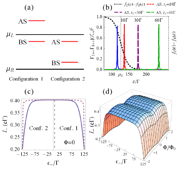
Figure 15: (a) The schematic plot of the energy levels of the bonding and antibonding states in configuration 1 and 2 with the chemical potential of the left and right leads, $\mu_{L}$ and $\mu_{R}$. (b) The difference of the left and right lead particle distributions, $f_{L}(\varepsilon)-f_{R}(\varepsilon)$, and the effective transmission coefficients of the bonding and antibonding channels in configuration 1 for different interdot coupling $t_{c}$ are plotted. In this case, the energy $\epsilon_{-}$ of the bonding state is fixed at $115\Gamma$, and the corresponding transmission is plotted with the blue line. The transmissions of the antibonding state for $t_{c}=10,30,60\Gamma$ are plotted with the red dashed line, purple long dashed line, and green dot-dashed line, respectively. (c) $I_{-}$ as a function of $\epsilon_{-}$ is plotted. The blue solid line is for temperature $k_{B}T=10\Gamma$, and the purple dashed line is for zero temperature. The numbers 1, 2 in the plot denote the corresponding energy configurations 1 and 2 for $\left|t_{c}\right|=60\Gamma$. (d) $I_{-}$ is plotted as a function of $\epsilon_{-}$ and $\Phi$ Liu2016 .

In configuration 1, the current flowing through the bonding state channel, denoted by $I_{1-}$, is dominant such that the total current is almost given by $I\simeq I_{1-}$, where the current $I_{1+}$ flowing through the antibonding state channel in configuration 1 is negligible. In configuration 2, the total current $I_{2}=I_{2+}+I_{2-}+I_{2+-}$, where $I_{2+}$, $I_{2-}$ are the currents flowing through the antibonding and bonding state channels in configuration 2, respectively, and $I_{2+-}$ is the current due to the interference between the bonding and antibonding state channels. The latter is negligible in the weak indirect coupling regime Kubo2006 . Therefore, the total current in configuration 2 is mainly given by $I_{2}\simeq I_{2+}+I_{2-}$. With the assumption that currents flowing through the bonding state channel in configuration 1 and 2 are almost the same Hatano2011 , $I_{1-}\simeq I_{2-}$, one can determine the currents flowing through the bonding and antibonding state channels, respectively by the total currents measured separately in configuration 1 and 2. This is the method used in Ref. Hatano2011 for analysing the currents flowing through the bonding and antibonding state channels.

For the above experimental analysis, one shall ask that whether the current $I_{1+}$ flowing through the antibonding channel in configuration 1 is really negligible; and what are the conditions that should be satisfied such that the assumption $I_{1-}\approx I_{2-}$ is valid. According to Eq. (181), $I_{1+}$ depends on the overlap of the difference of particle number distributions in the two leads, $f_{L}(\varepsilon)-f_{R}(\varepsilon)$, with the effective transmission coefficient of antibonding state channel, $\Gamma_{L++}\Gamma_{R++}\left|G_{++}^{R}(\varepsilon)\right|^{2}$. In Fig. 15(b), the difference $f_{L}(\varepsilon)-f_{R}(\varepsilon)$ is shown by the black dashed line. The energy of the bonding state is theoretically fixed, $\epsilon_{-}=\epsilon_{0}-|t_{c}|$, and the interdot coupling $t_{c}$ is changed to compare the corresponding antibonding state channel contributions to the current. In experiments, $\epsilon_{-}$ can be manipulated through tuning the energy of DQDs and the interdot coupling simultaneously. The effective transmission coefficient $\Gamma_{L--}\Gamma_{R--}\left|G_{--}^{R}(\varepsilon)\right|^{2}$ of the bonding state channel is fixed because of constant $\epsilon_{-}$, which is shown by the blue peak in Fig. 15(b). Other peaks are the corresponding effective transmission coefficient $\Gamma_{L++}\Gamma_{R++}\left|G_{++}^{R}(\varepsilon)\right|^{2}$ of the antibonding state channel for different $t_{c}$. As shown by Fig. 15(b), the larger $t_{c}$ gives the smaller overlap of $f_{L}(\varepsilon)-f_{R}(\varepsilon)$ with $\Gamma_{L++}\Gamma_{R++}\left|G_{++}^{R}(\varepsilon)\right|^{2}$ and hence the smaller current $I_{1+}$ flowing through the antibonding state channel in configuration 1. So one can conclude that $I_{1+}$ is negligible when $t_{c}$ is properly large enough to make $\Gamma_{L++}\Gamma_{R++}\left|G_{++}^{R}(\varepsilon)\right|^{2}$ lesser overlap with $f_{L}(\varepsilon)-f_{R}(\varepsilon)$ Liu2016 .

On the other hand, the current $I_{-}$ flowing through the bonding state channel as a function of the energy $\epsilon_{-}$ of the bonding state is shown in Fig. 15(c). Figure 15(c) shows that the current $I_{-}$ flowing through the bonding state channel becomes maximum when the energy $\epsilon_{-}$ of the bonding state is located in the middle of the bias window. The current $I_{-}$ symmetrically and dramatically decays when $\epsilon_{-}$ approaches closely to $\mu_{L}$ or $\mu_{R}$. In Fig. 15(c), the blue solid line gives the current $I_{-}$ as a function of $\epsilon_{-}$ for temperature $k_{B}T=10\Gamma$. It shows that $I_{-}$ is almost a constant within $\left|\epsilon_{-}\right|\lesssim 80\Gamma$. This indicates that the condition $I_{1-}\simeq I_{2-}$ is well satisfied for $\left|\epsilon_{-}\right|\lesssim 80\Gamma$. The purple dashed line in Fig. 15(c) shows $I_{-}$ at zero temperature . In this case, the range for $I_{-}$ being almost a constant is wider. Also, this flat pattern is maintained for arbitrary magnetic flux $\Phi$ (see Fig.15(d)).

The experiment of Ref. Hatano2011 was performed under wide band limit, weak coupling, and large bias regime, which is a typical regime for transport experiment of DQDs devices. As shown in Eq. (115), the steady-state single-particle reduced density matrix in the wide band limit is simply given by $\rho^{(1)}(t\rightarrow\infty)=\bm{v}(t,t\rightarrow\infty)$. Because of the indirect interdot weak coupling (small $a_{L,R}$), one can ignore the higher order terms of $a_{L,R}$ Liu2016 . The steady-state diagonal elements $v_{\pm\pm}$ then have the simple forms as:

$$v_{\pm\pm} \simeq\int_{-\infty}^{+\infty}\frac{d\varepsilon}{2\pi}\sum_{\alpha=L,R}f_{\alpha}(\varepsilon)\Gamma_{\alpha\pm\pm}\left|G_{\pm\pm}^{R}(\varepsilon)\right|^{2},$$

$$=v_{L\pm\pm}+v_{R\pm\pm}.$$ (183)

The steady-state transport currents through the bonding and antibonding state channels given in Eq. (181) can be approximately expressed in terms of $v_{\alpha\pm\pm}$

$$I_{\pm}=e\Gamma_{R\pm\pm}v_{L\pm\pm}-e\Gamma_{L\pm\pm}v_{R\pm\pm}.$$ (184)

From the above results, one obtains the relations between occupation numbers of the bonding and antibonding states and the corresponding currents approximately:

$$\rho^{(1)}_{\pm\pm}\simeq\frac{I_{\pm}}{e\Gamma_{R\pm\pm}}.$$ (185)

The comparison between this approximated solution with the exact one given by Eqs. (174) and (175) at the steady-state limit $t\rightarrow\infty$ are presented in Fig. 16(a), where energy configuration $\epsilon_{-}=-40\Gamma$ is chosen as an example. As one see, the approximation solution is almost the same as the exact one. Equation (185) implies that the currents flowing through the bonding or antibonding state channels can be used to determine the particle occupations in the corresponding state. The bonding and antibonding state components of the retarded Green function $|G_{\pm\pm}^{R}(\varepsilon)|^{2}$ in Eq. (183) have sharp peaks located at $\epsilon_{\pm}$, respectively, as the effective transmission shown in Fig. 15. When the bias is large ($\epsilon_{\pm}\gg\mu_{R}$), $v_{R\pm\pm}$ are ignorable. This is because electrons in the right lead hardly tunnel back into DQDs. The off-diagonal elements $v_{\pm\mp}$ relates to the tunneling probability between the bonding and antibonding states. Because there is no direct coupling between the bonding and antibonding states, the electrons must hop to the leads, then hop back to the other state. The weak couplings to the leads suppress the probability, and hence $v_{\pm\mp}$ are ignorable, as shown in Fig. 16(b) in which the magnitude of $v_{+-}$ is the order of $10^{-3}$ of the magnitude of the diagonal elements. Consequently, the reduced density matrix of Eq. (176) in the steady-state limit can be approximately given by the bonding and antibonding currents:

$$\rho_{00}\simeq\Big{(}1-\frac{I_{+}}{e\Gamma_{R++}}\Big{)}\Big{(}1-\frac{I_{-}}{e\Gamma_{R--}}\Big{)},$$ (186a)

$$\rho_{--}\simeq\frac{I_{-}}{e\Gamma_{R--}}\Big{(}1-\frac{I_{+}}{e\Gamma_{R++}}\Big{)},$$ (186b)

$$\rho_{++}\simeq\frac{I_{+}}{e\Gamma_{R++}}\Big{(}1-\frac{I_{-}}{e\Gamma_{R--}}\Big{)},$$ (186c)

$$\rho_{dd}\simeq\frac{I_{+}}{e\Gamma_{R++}}\frac{I_{-}}{e\Gamma_{R--}},$$ (186d)

$$\rho_{+-}=v_{+-}\simeq 0.$$ (186e)

The comparison between the above approximated solution with the exact elements of Eq. (176) in the steady-state limit is shown in Fig. 16(c), which give almost the same results between the approximated solution and the exact one.

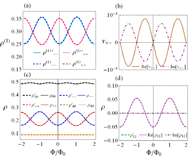
Figure 16: (a) The exact and approximate occupation numbers given by Eq. (185) in the bonding and antibonding states. (b) The real part and the imaginary part of $v_{+-}$ ($\rho_{+-}$). (c) The exact and approximate diagonal elements given by Eq. (186) of the reduced density matrix in the molecular basis. (d) The exact and approximate off-diagonal reduced density matrix elements in the dot basis Liu2016 .

For practical application of DQDs as a promising qubit, one is interested in the quantum coherence between the two physical dots, which is described by the off-diagonal matrix element $\rho_{12}(t)$ in the physical dot basis. The reduced density matrix elements in the physical dot basis (the charge qubit basis) of the DQDs is given by the following relation Tu2008 ; Tu2012a :

$$\rho_{12}(t) =\frac{1}{2}\big{(}\rho_{--}(t)-\rho_{++}(t)\big{)}+i~{}\!\textrm{Im}\rho_{+-}(t),$$ (187a)

$$\simeq\frac{1}{2}\big{(}\rho_{--}(t)-\rho_{++}(t)\big{)}.$$

$$\rho_{{}^{1}_{2}{}^{1}_{2}}(t) =\frac{1}{2}\big{(}\rho_{--}(t)+\rho_{++}(t)\big{)}\pm\textrm{Re}\rho_{+-}(t),$$ (187b)

$$\simeq\frac{1}{2}\big{(}\rho_{--}(t)+\rho_{++}(t)\big{)}.$$

The off-diagonal element $\rho_{12}(t)$ is presented in Fig. 16(d). In the charge qubit basis, the probability of the diagonal elements, $\rho_{11}(t)$ and $\rho_{22}(t)$ can also be determined from the diagonal density matrix element, $\rho_{--}$ and $\rho_{++}$ of the bonding and antibonding states, as shown in the above equation. Thus, the complete information of the reduced density matrix of the DQDs can be obtained experimentally from the measured currents through the relations given by Eqs. (186) and (187).

IV Conclusion

In summary, we have established a non-equilibrium quantum theory for the transient electron dynamics of various nanodevices, based on the path integral method in the fermion coherent-state representation. Our theory builds on the master equation of the reduced density matrix. The non-equilibrium transport current is directly derived from the reduced density matrix. The master equation for the reduced density matrix (i.e. equation (II.3), which provides all the information about the electron quantum coherence in the device) plus the transient current (i.e. equation (II.3), which determines transient electron transport phenomena) together provide a unique procedure to address the quantum decoherence problem in nonequilibrium quantum transport. The master equation takes a convolutionless form and hence the non-Markovian dynamics are fully encoded in the time-dependent coefficients. Explicitly, the back-reaction effect of the gating electrodes on the central system is fully taken into account by these time-dependent coefficients through the integrodifferential equations of motion (108) for the nonequilibrium Green functions. The non-Markovian memory structure is non-perturbatively built into the integral kernels in these equations of motion. All the physical observables can be calculated directly from the master equation. In particular, the transient transport current (II.3), and the single particle density matrix, (115), are found directly from the master equation in a rather simple way. The master equation and the transient transport current are also explicitly related to each other in terms of the superoperators acting on the reduced density matrix [see equation (II.3)].

This exact non-equilibrium formalism should provide a very intuitive picture showing how the change in the electron quantum coherence in the devices is intimately related to the electron tunneling processes through the leads and therefore responds nonlinearly to the corresponding external bias and gate controls. This theory is applicable to a variety of quantum decoherence and quantum transport phenomena involving non-Markovian memory effects, in both stationary and transient scenarios, and at arbitrary initial temperatures of the different contacts. The examples are given in Sec. III. As we have also presented, one can simply reproduce the non-equilibrium transport theory in terms of the non-equilibrium Green function technique from the master equation formalism. However, we should point out that the quantum transport theory based on the non-equilibrium Green function technique does not explicitly give the connection to the reduced density matrix of the device and thereby lacks a direct description of the quantum decoherence processes of the electrons and the non-Markovian memory dynamics in nanostructures. Besides, the master equation approach can be easily extended to incorporate the initial correlations, the formula for the master equation and the transient current remain unchanged, the only change is given by the system-lead nonlocal time correlation (144) and (145) in the determination of the correlation Green function (143).

References

- (1) M. A. Kastner, Artificial Atoms, Physics Today 46(1), 24 (1993)
- (2) L. L. Chang, L. Esaki, and R. Tsu, Resonant tunneling in semiconductor double barriers, Appl. Phys. Lett. 24(12), 593 (1974)
- (3) T. Ando, A. B. Fowler, and F. Stern, Electronic properties of two-dimensional systems, Rev. Mod. Phys. 54(2), 437 (1982)
- (4) E. R. Brown, J. R. Soderstrom, C. D. Parker, L. J. Mahoney, K. M. Molvar, and T. C. McGill, Oscillations up to 712 GHz in InAs/AlSb resonant?tunneling diodes, Appl. Phys. Lett. 58(20), 2291 (1991)
- (5) K. v. Klitzing, G. Dorda, and M. Pepper, New Method for High-Accuracy Determination of the Fine-Structure Constant Based on Quantized Hall Resistance, Phys. Rev. Lett. 45(6), 494 (1980)
- (6) Y. Imry, Introduction to Mesoscopic Physics, (2nd Ed. Oxford, 2002)
- (7) M. Büttiker, Scattering theory of current and intensity noise correlations in conductors and wave guides, Phys. Rev. B 46(19), 12485 (1992)
- (8) H. Ohnishi, T. Inata, S. Muto, N. Yokoyama, and A. Shibatomi, Self?consistent analysis of resonant tunneling current, Appl. Phys. Lett. 49(19), 1248 (1986)
- (9) A. Szafer and A. D. Stone, Theory of Quantum Conduction through a Constriction, Phys. Rev. Lett. 62(3), 300(1989)
- (10) J. Schwinger, Brownian Motion of a Quantum Oscillator, J. Math. Phys. (N.Y.) 2(3), 407 (1961)
- (11) L.P. Kadanoff and G. Baym, Quantum Statistical Mechanics (Benjamin, New York, 1962)
- (12) K. C. Chou, Z.-B. Su, B.-L. Hao, L. Yu, Equilibrium and nonequilibrium formalisms made unified, Phys. Rep. 118(1-2), 1 (1985)
- (13) J. Rammer and H. Smith, Quantum field-theoretical methods in transport theory of metals, Rev. Mod. Phys. 58(2), 323 (1986)
- (14) J. S. Wang, B. K. Agarwalla, H. Li, J. Thingna, Nonequilibrium Green s function method for quantum thermal transport, Front. Phys. 9(6), 673 (2014)
- (15) H. Haug and A. P. Jauho, Quantum Kinetics in Transport and Optics of Semiconductors (Springer Series in Solid-State Sciences Vol. 123, 2008)
- (16) N. S. Wingreen, A. P. Jauho and Y. Meir, Time-dependent transport through a mesoscopic structure, Phys. Rev. B 48(11), 8487 (1993)
- (17) A. P. Jauho, N. S. Wingreen, and Y. Meir, Time-dependent transport in interacting and noninteracting resonant-tunneling systems, Phys. Rev. B 50(8), 5528 (1994)
- (18) H. Schoeller and G. Schön, Mesoscopic quantum transport: Resonant tunneling in the presence of a strong Coulomb interaction, Phys. Rev. B 50(24), 18436 (1994)
- (19) S. A. Gurvitz and Ya. S. Prager, Microscopic derivation of rate equations for quantum transport, Phys. Rev. B 53(23), 15932 (1996)
- (20) J. S. Jin, X. Zheng, and Y. J. Yan, Exact dynamics of dissipative electronic systems and quantum transport: Hierarchical equations of motion approach, J. Chem. Phys. 128(23), 234703 (2008)
- (21) M. W. -Y. Tu and W. M. Zhang, Non-Markovian decoherence theory for a double-dot charge qubit, Phys. Rev. B 78(23), 235311 (2008)
- (22) M. W. -Y. Tu, M.-T. Lee, and W. M. Zhang, Exact master equation and non-markovian decoherence for quantum dot quantum computing, Quantum Inf. Processing (Springer) 8, 631 (2009)
- (23) J. S. Jin, M. W. Y. Tu, W. M. Zhang, and Y. J. Yan, Non-equilibrium quantum theory for nanodevices based on the Feynman VVernon influence functional ,New J. Phys. 12(8), 083013 (2010)
- (24) X. Q. Li, Number-resolved master equation approach to quantum measurement and quantum transport, Front. Phys. 11(4), 110307 (2016)
- (25) Y. J. Yan, J. S. Jin, R. X. Xu, X. Zheng, Dissipation equation of motion approach to open quantum systems, Front. Phys. 11 (4), 110306 (2016)
- (26) S. Datta, Electronic Transport in Mesoscopic Systems (Cambridge, 1995)
- (27) R. Landauer, Spatial Variation of Currents and Fields Due to Localized Scatterers in Metallic Conduction, IBM J. Res. Dev. 1(3), 223 (1957)
- (28) R. Landauer, Electrical resistance of disordered one-dimensional lattices, emphPhilos. Mag. 21(172), 863 (1970)
- (29) M. Büttiker, Y. Imry, R. Landauer, and S. Pinhas, Generalized many-channel conductance formula with application to small rings, Phys. Rev. B 31(10), 6207 (1985)
- (30) M. Büttiker, Four-Terminal Phase-Coherent Conductance, Phys. Rev. Lett. 57(14), 1761 (1986)
- (31) Ya. M. Blanter, M. Büttiker, Shot noise in mesoscopic conductors, Phys. Rep. 336(1-2), 1 (2000)
- (32) M. Büttiker, Absence of backscattering in the quantum Hall effect in multiprobe conductors, Phys. Rev. B 38(14), 9375 (1988)
- (33) M. Büttiker, Quantized transmission of a saddle-point constriction, Phys. Rev. B 41(11), 7906 (1990)
- (34) P. Samuelsson and M. Büttiker, Quantum state tomography with quantum shot noise, Phys. Rev. B 73(4), 041305 (2006)
- (35) E. A. Rothstein, O. Entin-Wohlman, and A. Aharony, Noise spectra of a biased quantum dot, Phys. Rev. B 79(7), 075307 (2009)
- (36) M. Moskalets and M. Büttiker, Adiabatic quantum pump in the presence of external ac voltages, Phys. Rev. B 69(20), 205316 (2004)
- (37) O. Entin-Wohlman, A. Aharony, and Y. Levinson, Adiabatic transport in nanostructures, Phys. Rev. B 65(19), 195411 (2002)
- (38) M. Moskalets, and M. Buttiker, Time-resolved noise of adiabatic quantum pumps, Phys. Rev. B 75(3), 035315 (2007)
- (39) G. D. Mahan, Many Particle Physics (Plenum, New York, 1990), 2nd ed.
- (40) L.V. Keldysh, Diagram Technique for Nonequilibrium Processes, Zh. Eksp. Teor. Fiz. 47(4), 1515 (1964) [Sov. Phys. JETP 20(4), 1018 (1965)]
- (41) G. Stefanucci and C.-O.Almbladh, Time-dependent partition-free approach in resonant tunneling systems, Phys. Rev. B 69(19), 195318 (2004)
- (42) M. Cini, Time-dependent approach to electron transport through junctions: General theory and simple applications, Phys. Rev. B 22(12), 5887 (1980)
- (43) U. Fano, Effects of Configuration Interaction on Intensities and Phase Shifts, Phys. Rev. 124(6), 1866 (1961)
- (44) P. W. Anderson, Absence of Diffusion in Certain Random Lattices, Phys. Rev. 109(5), 1492 (1958)
- (45) C. Caroli, R. Combescot, P. Nozìeres, and D. Saint-James, Direct calculation of the tunneling current, J. Phys. C 4,916 (1971)
- (46) C. Caroli, R. Combescot, P. Nozìeres, and D. Saint-James, A direct calculation of the tunnelling current. II. Free electron description , J. Phys. C 4, 2598 (1971)
- (47) D. C. Langreth, Linear and Nonlinear Electron Transport in Solids, ed. by J. T. Devreese, E. Van Doren (Plenum, New York, 1976)
- (48) X. Q. Li, J. Luo, Y. G. Yang, P. Cui, and Y. J. Yan, Quantum master-equation approach to quantum transport through mesoscopic systems, Phys. Rev. B 71(20), 205304 (2005)
- (49) R. P. Feynman, and F. L. Vernon, The theory of a general quantum system interacting with a linear dissipative system Ann. Phys. (N.Y.) 24, 118 (1963)
- (50) W. M. Zhang, D. H. Feng, and R. Gilmore, Coherent states: Theory and some applications, Rev. Mod. Phys. 62(4), 867 (1990)
- (51) M. W. -Y. Tu, W. M. Zhang, and J. S. Jin, Intrinsic coherence dynamics and phase localization in nanoscale Aharonov-Bohm interferometers, Phys. Rev. B 83(11), 115318 (2011)
- (52) C. Y. Lin and W. M. Zhang, Single-electron turnstile pumping with high frequencies, Appl. Phys. Lett. 99(7), 072105 (2011)
- (53) M. W.-Y. Tu, W. M. Zhang, J. S. Jin, O. Entin-Wohlman, and A. Aharony, Transient quantum transport in double-dot Aharonov-Bohm interferometers, Phys. Rev. B 86(11), 115453 (2012)
- (54) M. W. -Y. Tu, W. M. Zhang, and F. Nori, Transient quantum transport in double-dot Aharonov-Bohm interferometers, Phys. Rev. B 86(11), 115453 (2012)
- (55) J. S. Jin, M. W. -Y. Tu, N. E. Wang, and W. M. Zhang, Precision control of charge coherence in parallel double dot systems through spin-orbit interaction, J. Chem. Phys. 139(6), 064706 (2013)
- (56) M. W.-Y. Tu, A. Aharony, W. M. Zhang, and O. Entin-Wohlman, Real-time dynamics of spin-dependent transport through a double-quantum-dot Aharonov-Bohm interferometer with spin-orbit interaction, Phys. Rev. B 90(16), 165422 (2014)
- (57) P. Y. Yang, C. Y. Lin, and W. M. Zhang, Transient current-current correlations and noise spectra, Phys. Rev. B 89(11), 115411 (2014)
- (58) P. Y. Yang, C. Y. Lin, W. M. Zhang, Master equation approach to transient quantum transport in nanostructures incorporating initial correlations, Phys. Rev. B 92(16), 165403 (2015)
- (59) M. W. -Y. Tu, A. Aharony, O. Entin-Wohlman, A. schiller, and W. M. Zhang, Transient probing of the symmetry and the asymmetry of electron interference, Phys. Rev. B 93(12), 125437 (2016)
- (60) J. H. Liu, M. W. Y. Tu, W. M. Zhang, Quantum coherence of the molecular states and their corresponding currents in nanoscale Aharonov-Bohm interferometers, Phys. Rev. B 94(4), 045403 (2016)
- (61) A. J. Leggett, S. Chakravarty, A. T. Dorsey, M. P. A. Fisher, A. Garg and W. Zwerger, Dynamics of the dissipative two-state system, Rev. Mod. Phys. 59(1), 1 (1987)
- (62) R. Landauer, Condensed-matter physics: The noise is the signal, Nature (London) 392, 658 (1998)
- (63) C. Beenakker and C. Schonenberger, Quantum shot noise, Phys. Today 56(5), 37 (2003)
- (64) T. Gramespacher and M. Büttiker, Quantum Shot Noise at Local Tunneling Contacts on Mesoscopic Multiprobe Conductors, Phys. Rev. Lett. 81(13), 2763 (1998)
- (65) L. Saminadayar, D. C. Glattli, Y. Jin, and B. Etienne, Observation of the e/3 Fractionally Charged Laughlin Quasiparticle, Phys. Rev. Lett. 79(13), 2526 (1997)
- (66) F. Lefloch, C. Hoffmann, M. Sanquer, and D. Quirion, Doubled Full Shot Noise in Quantum Coherent Superconductor-Semiconductor Junctions, Phys. Rev. Lett. 90(6), 067002 (2003)
- (67) R. J. Schoelkopf, P. J. Burke, A. A. Kozhevnikov, D. E. Prober, and M. J. Rooks, Frequency Dependence of Shot Noise in a Diffusive Mesoscopic Conductor, Phys. Rev. Lett. 78(17), 3370 (1997)
- (68) R. Deblock, E. Onac, L. Gurevich, and L. P. Kouwenhoven, Detection of Quantum Noise from an Electrically Driven Two-Level System, Science 301(5630), 203(2003)
- (69) E. Onac, F. Balestro, L. H. Willems van Beveren, U. Hartmann, Y. V. Nazarov, and L. P. Kouwenhoven, Using a Quantum Dot as a High-Frequency Shot Noise Detector, Phys. Rev. Lett. 96(17), 176601 (2006)
- (70) E. Zakka-Bajjani, J. Ségala, F. Portier, P. Roche, D. C. Glattli, A. Cavanna and Y. Jin, Experimental Test of the High-Frequency Quantum Shot Noise Theory in a Quantum Point Contact, Phys. Rev. Lett. 99(23), 236803 (2007)
- (71) N. Lambert, R. Auguado, and T. Brandes, Nonequilibrium entanglement and noise in coupled qubits, Pys. Rev. B 75(4), 045340 (2007)
- (72) R. Aguado and T. Brandes, Shot Noise Spectrum of Open Dissipative Quantum Two-Level Systems, Phys. Rev. Lett. 92(20), 206601 (2004)
- (73) B. H. Wu, and C. Timm, Noise spectra of ac-driven quantum dots: Floquet master-equation approach, Phys. Rev. B 81(7), 075309 (2010)
- (74) H. A. Engel and D. Loss, Asymmetric Quantum Shot Noise in Quantum Dots, Phys. Rev. Lett. 93(13), 136602 (2004)
- (75) O. Entin-Wohlman, Y. Imry, S. A. Gurvitz, and A. Aharony, Steps and dips in the ac conductance and noise of mesoscopic structures, Phys. Rev. B 75(19), 193308 (2007)
- (76) C. P. Orth, D. F. Urban, and A. Komnik, Finite-frequency noise properties of the nonequilibrium Anderson impurity model, Phys. Rev. B 86(12), 125324 (2012)
- (77) U. Gavish, Y. Levinson, and Y. Imry, Detection of quantum noise, Phys. Rev. B 62(16), 10637 (2000)
- (78) R. Aguado and L. P. Kouwenhoven, Double Quantum Dots as Detectors of High-Frequency Quantum Noise in Mesoscopic Conductors, Phys. Rev. Lett. 84(9), 1986 (2000)
- (79) P. Billangeon, F. Pierre, R. Deblock, and H. Bouchiat, Out of equilibrium noise in electronic devices: from the classical to the quantum regime, J. Stat. Mech. 1, 01041 (2009)
- (80) N. Ubbelohde, C. Fricke, C. Flindt, F. Hohls, and R. J. Haug, Measurement of finite-frequency current statistics in a single-electron transistor, Nat. Commun. 3, 612 (2012)
- (81) A. Zazunov, M. Creux, E. Paladino, A. Crépieux, and T. Martin, Detection of Finite-Frequency Current Moments with a Dissipative Resonant Circuit, Phys. Rev. Lett. 99(6), 066601 (2007)
- (82) Z. Feng, J. Maciejko, J. Wang, and H. Guo, Current fluctuations in the transient regime: An exact formulation for mesoscopic systems, Phys. Rev. B 77(7), 075302 (2008)
- (83) K. Joho, S. Maier, and A. Komnik, Transient noise spectra in resonant tunneling setups: Exactly solvable models, Phys. Rev. B 86(15), 155304 (2012)
- (84) R. Zwanzig, Nonequilibrium Statistical Mechanics (Oxford Univ. Press, New York, 2001)
- (85) G. F. Mazenlo, Nonequilibrium Statistics Mechanics (Wiley-VCH, Weinheim, 2006)
- (86) J. Maciejko, J. Wang, and H. Guo, Time-dependent quantum transport far from equilibrium: An exact nonlinear response theory, Phys. Rev. B 74(8), 085324 (2006)
- (87) W. Lu, Z. Ji, L. Pfeiffer, K. W. West, and A. J. Rimberg, Real-time detection of electron tunnelling in a quantum dot, Nature (London) 423, 422 (2003)
- (88) J. Bylander, T. Duty, and P. Delsing, Current measurement by real-time counting of single electrons, Nature (London) 434, 361 (2005)
- (89) S. Gustavsson, I. Shorubalko, R. Leturcq, S. Schön, and K. Ensslin, Measuring current by counting electrons in a nanowire quantum dot, Appl. Phys. Lett. 92(15), 152101 (2008)
- (90) G. Stefanucci, Bound states in ab initio approaches to quantum transport: A time-dependent formulation, Phys. Rev. B 75(19), 195115 (2007)
- (91) R. Kubo, S. J. Muyake, and N. Hashitsume, Solid State Physics, edited by H. Ehrenreich and D. Turnbull (Academic, New York, 1965),Vol. 17,p. 269.
- (92) C. Cercignani, Theory and Application of the Boltzmann Equation (Edinburgh: Scottish Academic Press, 1975)
- (93) H. Smith and H. H. Jensen, Transport Phenomena (Oxford: Clarendon, 1989)
- (94) P. Breuer and F. Petruccione, The Theory of Open Quantum Systems (Oxford University Press, New York, 2002)
- (95) S. Nakajima, On Quantum Theory of Transport Phenomena Steady Diffusion, Prog. Theo. Phys. 20(6), 948 (1958)
- (96) R. Zwanzig, Ensemble Method in the Theory of Irreversibility, J. Chem. Phys. 33(5), 1338 (1960)
- (97) P. Y. Yang, W. M. Zhang,Exact homogeneous master equation for open quantum systems incorporating initial correlations , arXiv:1605.08521 (2016)
- (98) H. L. Lai, W. M. Zhang, Non-Markovian decoherence dynamics of Majorana fermions (in preparation)
- (99) W. M. Zhang, P. Y. Lo, H. N. Xiong, M. W. Y. Tu, and F. Nori, General Non-Markovian Dynamics of Open Quantum Systems, Phys. Rev. Lett. 109(17), 170402 (2012)
- (100) X. L. Yin, M. W.-Y. Tu, P. Y. Lo, and W. M. Zhang, Localized state effect in quantum transport (in preparation)
- (101) S. P. Giblin, M. Kataoka, J. D. Fletcher, P. See, T. J. B. M. Janssen, J. P. Griffths, G. A. C. Jones, I. Farrer, and D. A. Ritchie, Towards a quantum representation of the ampere using single electron pumps, Nat. Commun. 3, 930 (2012)
- (102) P. Y. Lo, H. N. Xiong and W. M Zhang, Breakdown of Bose-Einstein distribution in photonic crystals, Sci. Rep. 5, 09423 (2015)
- (103) J. Taylor, H. Guo, and J. Wang, textitAb initio modeling of quantum transport properties of molecular electronic devices, Phys. Rev. B 63(24), 245407 (2001)
- (104) P. Pomorski, L. Pastewka, C. Roland, H. Guo, and J. Wang, Capacitance, induced charges, and bound states of biased carbon nanotube systems, Phys. Rev. B 69(11), 115418 (2004)
- (105) V. Vettchinkina, A. Kartsev, D. Karlsson, and C. Verdozzi, Interacting fermions in one-dimensional disordered lattices: Exploring localization and transport properties with lattice density-functional theories, Phys. Rev. B 87(11), 115117 (2013)
- (106) A. Dhar and D. Sen, Nonequilibrium Green s function formalism and the problem of bound states, Phys. Rev. B 73(8), 085119 (2006)
- (107) D. Loss and D. P. DiVincenzo, Quantum computation with quantum dots, Phys. Rev. A 57(1), 120 (1998)
- (108) T. Hayashi, T. Fujisawa, H. D. Cheong, Y. H. Jeong, and Y. Hirayama, Coherent Manipulation of Electronic States in a Double Quantum Dot, Phys. Rev. Lett. 91(22), 226804 (2003)
- (109) J. M. Elzerman, R. Hanson, J. S. Greidanus, L. H. Willems van Beveren, S. De Franceschi, L. M. K. Vandersypen, S. Tarucha, and L. P. Kouwenhoven, Few-electron quantum dot circuit with integrated charge read out, Phys. Rev. B 67(16), 161308(R) (2003)
- (110) J. R. Petta, A. C. Johnson, C. M. Marcus, M. P. Hanson, and A. C. Gossard, Manipulation of a Single Charge in a Double Quantum Dot, Phys. Rev. Lett. 93(18), 186802 (2004)
- (111) J. Gorman, D. G. Hasko, and D. A. Williams, Charge-Qubit Operation of an Isolated Double Quantum Dot, Phys. Rev. Lett. 95(9), 090502 (2005)
- (112) A. C. Johnson, J. R. Petta, J. M. Taylor, A. Yacoby, M. D. Lukin, C. M. Marcus, M. P. Hanson, and A. C. Gossard, Triplet Vsinglet spin relaxation via nuclei in a double quantum dot, Nature (London) 435, 925 (2005)
- (113) J. R. Petta, A. C. Johnson, J. M. Taylor, E. A. Laird, A. Yacoby, M. D. Lukin, C. M. Marcus, M. P. Hanson, and A. C. Gossard, Coherent Manipulation of Coupled Electron Spins in Semiconductor Quantum Dots, Science 309, 2180 (2005).
- (114) K. D. Petersson, C. G. Smith, D. Anderson, P. Atkinson, G. A. C. Jones, and D. A. Ritchie, Charge and Spin State Readout of a Double Quantum Dot Coupled to a Resonator, Nano Lett. 10, 2789 (2010).
- (115) B. M. Maune, et al., Coherent singlet-triplet oscillations in a silicon-based double quantum dot, Nature 481, 344 (2012)
- (116) L. Fricke, M. Wulf, B. Kaestner, V. Kashcheyevs, J. Timoshenko, P. Nazarov, F. Hohls, P. Mirovsky, B. Mackrodt, R. Dolata, T. Weimann, K. Pierz, and H. W. Schumacher, Counting Statistics for Electron Capture in a Dynamic Quantum Dot, Phys. Rev. Lett. 110(12), 126803 (2013)
- (117) Z. Shi, C. B. Simmons, D. R. Ward, J. R. Prance, X. Wu, T. S. Koh, J. K. Gamble, D. E. Savage, M. G. Lagally, M. Friesen, S. N. Coppersmith, and M. A. Eriksson, Fast coherent manipulation of three-electron states in a double quantum dot, Nat. Comms. 5, 3020 (2014)
- (118) T. Fujisawa, T. Hayashi, and S. Sasaki, Time-dependent single-electron transport through quantum dots, Rep. Prog. Phys. 69, 759 (2006)
- (119) R. Hanson, J. R. Petta, S. Tarucha, and L. M. K. Vandersypen, Spins in few-electron quantum dots, Rev. Mod. Phys. 79(4), 1217 (2007)
- (120) D. Kim, Z. Shi, C. B. Simmons, D. R. Ward, J. R. Prance, T. S. Koh, J. K. Gamble, D. E. Savage, M. G. Lagally, M. Friesen, S. N. Coppersmith, and M. A. Erikssom, Quantum control and process tomography of a semiconductor quantum dot hybrid qubit, Nature, 511, 70 (2014)
- (121) Y. Wu, X. Li, L. M. Duan, D. G. Steel, and D. Gammon, Density Matrix Tomography through Sequential Coherent Optical Rotations of an Exciton Qubit in a Single Quantum Dot, Phys. Rev. Lett. 96(8), 087402 (2006)
- (122) S. Foletti, H. Bluhm, D. Mahalu, V. Umansky, and A. Yacoby, Universal quantum control of two-electron spin quantum bits using dynamic nuclear polarization, Nature Phys. 5, 903 (2009)
- (123) J. Medford, J. Beil, J. M. Taylor, S. D. Bartlett, A. C. Doherty, E. I. Rashba, D. P. DiVincenzo, H. Lu, A. C. Gossard, and C. M. Marcus, Self-consistent measurement and state tomography of an exchange-only spin qubit, Nature Nanotechnol. 8, 654 (2013).
- (124) Y. Aharonov and D. Bohm, Significance of Electromagnetic Potentials in the Quantum Theory, Phys. Rev. 115(3), 485 (1959)
- (125) A. W. Holleitner, C. R. Decker, H. Qin, K. Eberl, and R. H. Blick, Coherent Coupling of Two Quantum Dots Embedded in an Aharonov-Bohm Interferometer, Phys. Rev. Lett. 87(25), 256802 (2001)
- (126) T. Hatano, M. Stopa, W. Izumida, T. Yamaguchi, T. Ota, and S. Tarucha, Aharonov VBohm oscillations for charge transport through two parallel quantum dots, Physica E (Amsterdam) 22, 534 (2004)
- (127) M. Sigrist, A. Fuhrer, T. Ihn, K. Ensslin, S. E. Ulloa, W. Wegscheider, and M. Bichler, Magnetic-Field-Dependent Transmission Phase of a Double-Dot System in a Quantum Ring, Phys. Rev. Lett. 93(6), 066802 (2004)
- (128) D. Loss and E. V. Sukhorukov, Probing Entanglement and Nonlocality of Electrons in a Double-Dot via Transport and Noise, Phys. Rev. Lett. 84(5), 1035 (2000)
- (129) K. Kang and S. Y. Cho, Tunable molecular resonances of a double quantum dot Aharonov VBohm interferometer, J. Phys. Condens. Matter 16(1), 117 (2004)
- (130) T. Kubo, Y. Tokura, T. Hatano, and S. Tarucha, Electron transport through Aharonov-Bohm interferometer with laterally coupled double quantum dots, Phys. Rev. B. 74(20), 205310 (2006)
- (131) T. Hatano, T. Kubo, Y. Tokura, S. Amaha, S. Teraoka, and S. Tarucha, Aharonov-Bohm Oscillations Changed by Indirect Interdot Tunneling via Electrodes in Parallel-Coupled Vertical Double Quantum Dots, Phys. Rev. Lett. 106(7), 076801 (2011)