Method of lines transpose: Energy gradient flows using direct operator inversion for phase field models

Matthew Causley Mathematics Department, Kettering University, Flint, MI 48504 mcausley@kettering.edu Hana Cho Department of Mathematics, Michigan State University, East Lansing, MI 48824 chohana@math.msu.edu  and  Andrew Christlieb Department of Mathematics, Michigan State University, East Lansing, MI 48824 andrewch@math.msu.edu
Abstract.

In this work, we develop an 𝒪(N)𝒪𝑁\mathcal{O}(N) implicit real space method in 1D and 2D for the Cahn Hilliard (CH) and vector Cahn Hilliard (VCH) equations, based on the Method Of Lines Transpose (MOLTT{}^{\text{T}}) formulation. This formulation results in a semi-discrete time stepping algorithm, which we prove is gradient stable in the H1superscript𝐻1H^{-1} norm.

The spatial discretization follows from dimensional splitting, and an 𝒪(N)𝒪𝑁\mathcal{O}(N) matrix-free solver, which applies fast convolution to the modified Helmholtz equation. We propose a novel factorization technique, in which fourth order spatial derivatives are incorporated into the solver. The splitting error is included in the nonlinear fixed point iteration, resulting in a high order, logically Cartesian (line-by-line) update. Our method is fast, but not restricted to periodic boundaries like the fast Fourier transform (FFT).

The basic solver is implemented using the Backward Euler formulation, and we extend this to both backward difference (BDF) stencils, implicit Runge Kutta (SDIRK) and spectral deferred correction (SDC) frameworks to achieve high orders of temporal accuracy. We demonstrate with numerical results that the CH, and VCH equations maintain gradient stability in one and two spatial dimensions. We also explore time-adaptivity, so that meta-stable states and ripening events can be simulated both quickly and efficiently.


Keywords: Method of Lines Transpose, Rothe’s method, Implicit Methods, Boundary Integral Methods, Alternating Direction Implicit Methods, ADI schemes, Unconditionally gradient schemes, Cahn-Hilliard, Functionalized Cahn-Hilliard.

1. Introduction

Many materials such as metals, ceramics, and polymers have physical properties which depend strongly on their microstructure. The morphology evolves during various physical processes, such as solidification, solid-state phase transformation, grain coarsening and grain growth. These processes are governed complex and nonlinear chemical reactions, and so the location and motion of phase interfaces typically evolve over long time scales. Consequently the phase-field method has become a consolidated tool for simulating microstructure evolution. See [8] for a survey on the subject.

One of the most well-known phase field models is the Cahn-Hilliard (CH) equation. Cahn and Hilliard [3] introduced it to explain the phase separation by predicting the interfacial free energy between two coexisting phases. The free energy is modeled using an order parameter u𝑢u, and a reaction term f(u)𝑓𝑢f(u). The reaction function is defined as the derivative of a double-well potential with two minima, u=±1𝑢plus-or-minus1u=\pm 1, which represent each phase of the composite material. The phases are separated by transition layers, which are of width 𝒪(ϵ)𝒪italic-ϵ\mathcal{O}(\epsilon). The CH equation has been used extensively to model phenomena in material science; and several generalizations have been developed, including the vector Cahn-Hilliard (3) and functionalized Cahn-Hilliard equations.

In this paper, we will develop numerical schemes for phase field models based on the Method of Lines Transpose (MOLT) framework. The MOLTT{}^{\text{T}} formulation, which is a practical approach to Rothe’s method [21], starts by discretizing a PDE in time, and then developing efficient approaches to solve the resulting set of coupled boundary value problems. The traditional formulation, proposed by Rothe [21], resulted in large matrices that were cumbersome; hence the method did not get a great deal of attention. In the late 2000s Rothe’s method received more attention, due to the development of spectral deferred correction methods and Krylov subspace techniques [17]. Soon, other fast summation techniques such as the fast multipole method [19] were employed based on potential theory and boundary integral techniques.

Even more recently, MOLTT{}^{\text{T}} algorithms for PDEs have been developed in the context of wave propagation [4, 7, 5], in which the resulting Helmholtz boundary value problem is solved with a dimensionally split algorithm, similar to alternating direction implicit (ADI) methods [12, 15]. Here the spatial operator is inverted one dimension at a time through fast convolution, in a logically Cartesian fashion. In [7], successive convolution was introduced, leading to an A-stable method of arbitrary order in time for hyperbolic problems. This led the current authors to revisit this idea in context of linear and nonlinear (second order) parabolic problems [6], and successive convolution was inserted into the resolvent expansion of pseudo differential operators to achieve L-stable real space solvers which scale as 𝒪(N)𝒪𝑁\mathcal{O}(N) for N𝑁N spatial points.

Here we turn our attention to parabolic problems of higher order, specifically the CH equation and its extensions. To this end, we highlight the relevant new features of our approach:

  1. i

    We combine our previous work on the MOLTT{}^{\text{T}} formulation [4, 7, 5, 6] with traditional implicit time stepping methods (BDF, SDIRK and IDC methods, with time adaptivity);

  2. ii

    we directly invert the linear part of the differential operator using the Green’s function, combined with fast 𝒪(N)𝒪𝑁\mathcal{O}(N) convolution;

  3. iii

    we use dimensional splitting to avoid boundary integrals, and the need for global inversion;

  4. iv

    we directly include the splitting error in our formulation by explicitly incorporating it into the nonlinear iterations;

  5. v

    we remain competitive with explicit methods in terms of wall clock time needed to solve each fixed point iteration.

It is worth pointing out that the MOLTT{}^{\text{T}} formulation is really targeted at developing new paradigms for parallel multicore computing. The point to this paper, as well as our previous work, is to establish the theoretical and practical underpinnings necessary to address a wide class of PDEs. In particular, our task is to investigate the implementation for higher order PDEs. Parallel implementation will be the focus of our upcoming work in this area.

The rest of this organized as follows. In Section 2, we present several models which are of interest in this work. In Section 3, we derive a first order scheme for CH equation in a basic 1D setting.

In Section 4, we modify the traditional time stepping scheme, to achieve higher orders of accuracy and present temporal refinement studies. In addition, we extend 1D schemes to multiple spatial dimension in Section 5. Finally, we describe an adaptive time stepping strategy in Section 6 and present numerous numerical results including 1D, 2D solutions to the CH equations and the vector CH model in Section 7, followed by some concluding remarks.

2. Models

In this paper, we present the proposed Method of lines transpose (MOLTT{}^{\text{T}}) scheme for Cahn-Hilliard (CH) equation

ut=Δ[ϵ2Δuf(u)],𝐱Ωd,formulae-sequencesubscript𝑢𝑡Δdelimited-[]superscriptitalic-ϵ2Δ𝑢𝑓𝑢𝐱Ωsuperscript𝑑u_{t}=-\Delta\left[\epsilon^{2}\Delta u-f(u)\right],\quad{\bf x}\in\Omega\subset\mathbb{R}^{d}, (1)

with the appropriate initial and boundary conditions. The phase function uH1(Ω)𝑢superscript𝐻1Ωu\in H^{1}(\Omega) describes the volume fraction of one component of a binary mixture where H1(Ω)superscript𝐻1ΩH^{1}(\Omega) is the standard Sobolev space. The reaction function f(u)𝑓𝑢f(u) is the derivative of classical Ginzburg-Landau double-well potential F(u)=14(u21)2𝐹𝑢14superscriptsuperscript𝑢212F(u)=\frac{1}{4}(u^{2}-1)^{2} whose local minima is at u=±1𝑢plus-or-minus1u=\pm 1. The small parameter 0<ϵ10italic-ϵmuch-less-than10<\epsilon\ll 1 is the width of the interfacial transition layer. In a 1D setting (Ω[a,b]Ω𝑎𝑏\Omega\equiv[a,b]\subset\mathbb{R}), the Laplacian ΔΔ\Delta in the above equations is replaced by xxsubscript𝑥𝑥\partial_{xx}.

The CH equation (1) describes the H1superscript𝐻1H^{-1} gradient flow of the CH free energy [3]

(u)=Ωϵ22|u|2+F(u)d𝐱.𝑢subscriptΩsuperscriptitalic-ϵ22superscript𝑢2𝐹𝑢𝑑𝐱\mathcal{E}(u)=\int_{\Omega}\frac{\epsilon^{2}}{2}|\nabla u|^{2}+F(u)d{\bf x}. (2)

If we assume zero-flux boundary conditions, the CH free energy is dissipative

ddt(u)=ut,δδuL20.𝑑𝑑𝑡𝑢subscriptsubscript𝑢𝑡𝛿𝛿𝑢superscript𝐿20\frac{d}{dt}\mathcal{E}(u)=\left<u_{t},\frac{\delta\mathcal{E}}{\delta u}\right>_{L^{2}}\leq 0.

We emphasize that the physical property of energy stability is vital, and any consistent numerical scheme for the CH model must also possess this property. Many such schemes have been proposed, such as the operator splitting approach introduced by Eyre [14], the semi-implicit spectral deferred correction method by Shen, [22, 20], and even fully implicit schemes utilizing nonlinear solvers, such as the conjugate gradient method [9]. We shall use a linearly implicit fixed point method to solve the CH equation, which is stabilized by shifting the phase field about the background state u=1𝑢1u=-1.

We also consider vector version of CH (VCH) equation [9]. For 𝐮=(u1,u2)𝐮subscript𝑢1subscript𝑢2{\bf u}=(u_{1},u_{2}),

𝐮t=Δ[ϵ2Δ𝐮𝐮W(𝐮)]subscript𝐮𝑡Δdelimited-[]superscriptitalic-ϵ2Δ𝐮subscript𝐮𝑊𝐮{\bf u}_{t}=-\Delta\left[\epsilon^{2}\Delta{\bf u}-\nabla_{\bf u}W({\bf u})\right] (3)

where the reaction term is the derivative of the potential function,

W(𝐮)=Πi=13|𝐮𝐳i|2,𝐳i:cube roots of unity in the (u1,u2) plane.:𝑊𝐮superscriptsubscriptΠ𝑖13superscript𝐮subscript𝐳𝑖2subscript𝐳𝑖cube roots of unity in the subscript𝑢1subscript𝑢2 planeW({\bf u})=\Pi_{i=1}^{3}|{\bf u}-{\bf z}_{i}|^{2},\qquad{\bf z}_{i}:\text{cube roots of unity in the }(u_{1},u_{2})\text{ plane}. (4)

The potential W𝑊W is non-negative and its minimum values are attained at three vectors {𝐳i}subscript𝐳𝑖\{{\bf z}_{i}\}, so as to model a three-phase physical system. This model can be seen as the higher order volume preserving version of the vector-valued Ginzber-Landau equation [2] , which suggests a model for three phase boundary motion, such as the grain-boundary motion in alloys. The energy functional is a vector version of (2) such that

VCH(𝐮)=Ωϵ22|𝐮|2+W(𝐮)d𝐱.subscript𝑉𝐶𝐻𝐮subscriptΩsuperscriptitalic-ϵ22superscript𝐮2𝑊𝐮𝑑𝐱\mathcal{E}_{VCH}({\bf u})=\int_{\Omega}\frac{\epsilon^{2}}{2}|\nabla{\bf u}|^{2}+W({\bf u})d{\bf x}. (5)

3. First order scheme in one spatial dimension

Before employing a time discretization to CH equation (1), we first introduce a new transformed variable v=u+1𝑣𝑢1v=u+1. Since pure states u=±1𝑢plus-or-minus1u=\pm 1 dominates the solution during ripening, we see that equivalently v=0𝑣0v=0, 2. This transformation is partially motivated by [11], in which the same approach is combined with operator splitting to produce a contractive operator. Similarly, in [9] the linearized variable vu+1𝑣𝑢1v\approx u+1 is used as a preconditioner for the full problem. Our work is distinct, however in that we are not solving the linearized equation, but instead the fully nonlinear equation

vt=ϵ2vxxxx+f(v1)xx,f(v1)=v33v2+2v,formulae-sequencesubscript𝑣𝑡superscriptitalic-ϵ2subscript𝑣𝑥𝑥𝑥𝑥𝑓subscript𝑣1𝑥𝑥𝑓𝑣1superscript𝑣33superscript𝑣22𝑣v_{t}=-\epsilon^{2}v_{xxxx}+f(v-1)_{xx},\quad f(v-1)=v^{3}-3v^{2}+2v, (6)

which follows from the transformation v=u+1𝑣𝑢1v=u+1 inserted into the CH equation (1), with Ω=(a,b)Ω𝑎𝑏\Omega=(a,b). Similarly, the energy functional (2) becomes

(v)=abϵ22|vx|2+F(v1)d𝐱,F(v1)=14v4v3+v2formulae-sequence𝑣superscriptsubscript𝑎𝑏superscriptitalic-ϵ22superscriptsubscript𝑣𝑥2𝐹𝑣1𝑑𝐱𝐹𝑣114superscript𝑣4superscript𝑣3superscript𝑣2\mathcal{E}(v)=\int_{a}^{b}\frac{\epsilon^{2}}{2}|v_{x}|^{2}+F(v-1)d{\bf x},\quad F(v-1)=\frac{1}{4}v^{4}-v^{3}+v^{2} (7)

In Section 3.1, we will formulate our first-order MOLTT{}^{\text{T}} scheme using above equation (6), and will show that this transformation makes our scheme gradient stable in Section 3.1.1.

3.1. Semi-discrete scheme for 1D CH equation

We utilize the MOLT by discretizing (6) in time as the Backward Euler (BE) scheme,

vn+1vnΔt=ϵ2xxxxvn+1+2xxvn+1+xxf~n+1,f~(v)=v33v2,formulae-sequencesuperscript𝑣𝑛1superscript𝑣𝑛Δ𝑡superscriptitalic-ϵ2subscript𝑥𝑥𝑥𝑥superscript𝑣𝑛12subscript𝑥𝑥superscript𝑣𝑛1subscript𝑥𝑥superscript~𝑓𝑛1~𝑓𝑣superscript𝑣33superscript𝑣2\dfrac{v^{n+1}-v^{n}}{\Delta t}=-\epsilon^{2}\partial_{xxxx}v^{n+1}+2\partial_{xx}v^{n+1}+\partial_{xx}\tilde{f}^{n+1},\quad\tilde{f}(v)=v^{3}-3v^{2}, (8)

where vn=u(x,tn)+1superscript𝑣𝑛𝑢𝑥superscript𝑡𝑛1v^{n}=u(x,t^{n})+1 and Δt=tn+1tnΔ𝑡superscript𝑡𝑛1superscript𝑡𝑛\Delta t=t^{n+1}-t^{n}. This scheme (8) is first-order in time but still continuous in space. We note that the equation contains both linear and nonlinear implicit terms, and so an efficient iterative scheme is required to construct a fully implicit solution. We will suggest two nonlinear iteration schemes to solve the solution vn+1superscript𝑣𝑛1v^{n+1} in Section 3.1.2. We first prove that the semi-discrete solution of (8) is unconditionally gradient stable.

3.1.1. Energy stability

Our proof is similar to those which have appeared elsewhere [22, 14], in that we utilize the H1superscript𝐻1H^{-1}, under reasonable assumptions. However, we investigate the fully implicit scheme (8), which alters the linear part of the PDE. We first make useful observations.

  • The operator Δ1:{vL2|Ωv𝑑x=0}H2(Ω):superscriptΔ1conditional-set𝑣superscript𝐿2subscriptΩ𝑣differential-d𝑥0superscript𝐻2Ω\Delta^{-1}:\left\{v\in L^{2}|\int_{\Omega}vdx=0\right\}\rightarrow H^{2}(\Omega) is defined [11] as

    Δ1v=h<v,q>=<Δh,q>,qL2(Ω).\Delta^{-1}v=h\quad\Longleftrightarrow\quad<v,q>=<\Delta h,q>,\quad\forall q\in L^{2}(\Omega). (9)
  • For any p,qL2(Ω)𝑝𝑞superscript𝐿2Ωp,q\in L^{2}(\Omega), the following identity holds

    <p,pq>=12(p02q02+pq02)12(p02q02),formulae-sequenceabsent𝑝𝑝𝑞12superscriptsubscriptnorm𝑝02superscriptsubscriptnorm𝑞02superscriptsubscriptnorm𝑝𝑞0212superscriptsubscriptnorm𝑝02superscriptsubscriptnorm𝑞02<p,p-q>=\frac{1}{2}\left(\|p\|_{0}^{2}-\|q\|_{0}^{2}+\|p-q\|_{0}^{2}\right)\geq\frac{1}{2}\left(\|p\|_{0}^{2}-\|q\|_{0}^{2}\right), (10)

    where <,><\cdot,\cdot> is standard L2superscript𝐿2L^{2} inner product and 0\|\cdot\|_{0} is the L2superscript𝐿2L^{2} norm.

We will consider the first-order scheme (8) in general spatial dimension (Ωd,d)formulae-sequenceΩsuperscript𝑑𝑑(\Omega\in\mathbb{R}^{d},d\in\mathbb{N}).

Lemma 3.1.

Under the following assumption,

0v2,v=u+1formulae-sequence0𝑣2𝑣𝑢10\leq v\leq 2,\quad v=u+1

the fully-implicit scheme (8) satisfies the discrete energy law for any time step ΔtΔ𝑡\Delta t:

(vn+1)(vn),n0.formulae-sequencesuperscript𝑣𝑛1superscript𝑣𝑛for-all𝑛0\mathcal{E}(v^{n+1})\leq\mathcal{E}(v^{n}),\quad\forall n\geq 0.

where vnsuperscript𝑣𝑛v^{n} is approximation of v(x,tn)u(x,tn)+1𝑣𝑥superscript𝑡𝑛𝑢𝑥superscript𝑡𝑛1v(x,t^{n})\equiv u(x,t^{n})+1 of Cahn-Hilliard equation (1).

Proof.

The solution vn+1superscript𝑣𝑛1v^{n+1} satisfies the following weak formulation in H2(Ω)superscript𝐻2ΩH^{2}(\Omega),

1Δt<vn+1vn,ϕ>=ϵ2<Δvn+1,Δϕ>+2<vn+1,Δϕ>+<f~n+1,Δϕ>,\frac{1}{\Delta t}<v^{n+1}-v^{n},\phi>=-\epsilon^{2}<\Delta v^{n+1},\Delta\phi>+2<v^{n+1},\Delta\phi>+<\tilde{f}^{n+1},\Delta\phi>, (11)

for all ϕH2(Ω)italic-ϕsuperscript𝐻2Ω\phi\in H^{2}(\Omega). Utilizing (9), we choose the test function ϕ=Δ1(vn+1vn)italic-ϕsuperscriptΔ1superscript𝑣𝑛1superscript𝑣𝑛\phi=\Delta^{-1}(v^{n+1}-v^{n}), so that

1ΔtΔ1(vn+1vn)02=ϵ21Δ𝑡superscriptsubscriptnormsuperscriptΔ1superscript𝑣𝑛1superscript𝑣𝑛02superscriptitalic-ϵ2\displaystyle-\frac{1}{\Delta t}\|\nabla\cdot\Delta^{-1}(v^{n+1}-v^{n})\|_{0}^{2}=\epsilon^{2} <vn+1,(vn+1vn)>\displaystyle<\nabla v^{n+1},\nabla(v^{n+1}-v^{n})>
+2<vn+1,vn+1vn>+<f~n+1,vn+1vn>,\displaystyle+2<v^{n+1},v^{n+1}-v^{n}>+<\tilde{f}^{n+1},v^{n+1}-v^{n}>, (12)

where integration by parts is employed. Next we apply the identity (10),

0ϵ22(vn+102vn02)+(vn+102vn02+vn+1vn02)+<f~n+1,vn+1vn>.formulae-sequence0superscriptitalic-ϵ22superscriptsubscriptnormsuperscript𝑣𝑛102superscriptsubscriptnormsuperscript𝑣𝑛02limit-fromsuperscriptsubscriptnormsuperscript𝑣𝑛102superscriptsubscriptnormsuperscript𝑣𝑛02superscriptsubscriptnormsuperscript𝑣𝑛1superscript𝑣𝑛02superscript~𝑓𝑛1superscript𝑣𝑛1superscript𝑣𝑛absent0\geq\hskip 5.69054pt\frac{\epsilon^{2}}{2}(\|\nabla v^{n+1}\|_{0}^{2}-\|\nabla v^{n}\|_{0}^{2})+(\|v^{n+1}\|_{0}^{2}-\|v^{n}\|_{0}^{2}+\|v^{n+1}-v^{n}\|_{0}^{2})+<\tilde{f}^{n+1},v^{n+1}-v^{n}>. (13)

We replace the last term with its Taylor expansion

<F~n+1F~n,1>=<f~n+1,vn+1vn><f~(ξn+1)2(vn+1vn),vn+1vn>,<\tilde{F}^{n+1}-\tilde{F}^{n},1>=<\tilde{f}^{n+1},v^{n+1}-v^{n}>-<\frac{\tilde{f}^{\prime}(\xi^{n+1})}{2}(v^{n+1}-v^{n}),v^{n+1}-v^{n}>,

so that the inequality (13) becomes

(vn+1)(vn)superscript𝑣𝑛1superscript𝑣𝑛\displaystyle\mathcal{E}(v^{n+1})-\mathcal{E}(v^{n}) =ϵ22(vn+102vn02)+(vn+102vn02)+<F~n+1F~n,1>formulae-sequenceabsentsuperscriptitalic-ϵ22superscriptsubscriptnormsuperscript𝑣𝑛102superscriptsubscriptnormsuperscript𝑣𝑛02limit-fromsuperscriptsubscriptnormsuperscript𝑣𝑛102superscriptsubscriptnormsuperscript𝑣𝑛02superscript~𝐹𝑛1superscript~𝐹𝑛1absent\displaystyle=\frac{\epsilon^{2}}{2}(\|\nabla v^{n+1}\|_{0}^{2}-\|\nabla v^{n}\|_{0}^{2})+(\|v^{n+1}\|_{0}^{2}-\|v^{n}\|_{0}^{2})+<\tilde{F}^{n+1}-\tilde{F}^{n},1>
(f~21)vn+1vn020,absentsubscriptnormsuperscript~𝑓21superscriptsubscriptnormsuperscript𝑣𝑛1superscript𝑣𝑛020\displaystyle\leq\left(\frac{\|\tilde{f}^{\prime}\|_{\infty}}{2}-1\right)\|v^{n+1}-v^{n}\|_{0}^{2}\leq 0,

where \|\cdot\|_{\infty} is Lsuperscript𝐿L^{\infty} norm. The last inequality holds because f~=3v26v0superscript~𝑓3superscript𝑣26𝑣0\tilde{f}^{\prime}=3v^{2}-6v\leq 0 for 0v20𝑣20\leq v\leq 2. Therefore the discrete energy is non-increasing, and the implicit scheme (8) is unconditionally gradient stable. ∎

Remark 1.

In [22, 20], Shen et.al. introduced a stabilizing term S(un+1un)𝑆superscript𝑢𝑛1superscript𝑢𝑛S(u^{n+1}-u^{n}) for their semi-implicit scheme for the AC and CH equations. They choose the constant to satisfy Smaxu|f~(u)|2𝑆subscript𝑢superscript~𝑓𝑢2S\geq\dfrac{\max_{u\in\mathbb{R}}|\tilde{f}^{\prime}(u)|}{2} with the truncated potential 1u11𝑢1-1\leq u\leq 1. Equivalently, we assume that 0v20𝑣20\leq v\leq 2. However, we alter the linear part of the differential operator to ensure stability, rather than introducing an additional term.The distinction is that the transformation we employ modifies the linear part of the differential operator, rather than introducing an additional term, for stabilization.

3.1.2. Factorization of the linear operator

We will now propose a simple fixed point iterative solver for equation (8),

(I(2Δtxxϵ2Δtxxxx))vn+1,k+1=vn+Δtxxf~n+1,k,𝐼2Δ𝑡subscript𝑥𝑥superscriptitalic-ϵ2Δ𝑡subscript𝑥𝑥𝑥𝑥superscript𝑣𝑛1𝑘1superscript𝑣𝑛Δ𝑡subscript𝑥𝑥superscript~𝑓𝑛1𝑘\left(I-(2\Delta t\partial_{xx}-\epsilon^{2}\Delta t\partial_{xxxx})\right)v^{n+1,k+1}=v^{n}+\Delta t\partial_{xx}\tilde{f}^{n+1,k}, (14)

where k𝑘k indicates the iteration index. By lagging the the nonlinear term f~n+1,ksuperscript~𝑓𝑛1𝑘\tilde{f}^{n+1,k}, we can make the update explicit through formal analytic inversion of the fourth-order operator

vn+1,k+1=(I2Δtxx+ϵ2Δtxxxx)1[vn+Δtxxf~n+1,k].superscript𝑣𝑛1𝑘1superscript𝐼2Δ𝑡subscript𝑥𝑥superscriptitalic-ϵ2Δ𝑡subscript𝑥𝑥𝑥𝑥1delimited-[]superscript𝑣𝑛Δ𝑡subscript𝑥𝑥superscript~𝑓𝑛1𝑘v^{n+1,k+1}=\left(I-2\Delta t\partial_{xx}+\epsilon^{2}\Delta t\partial_{xxxx}\right)^{-1}\left[v^{n}+\Delta t\partial_{xx}\tilde{f}^{n+1,k}\right]. (15)

However, the Green’s function of this fourth order operator contain both decaying and oscillatory components, which would not produce an efficient method. Instead we propose a novel factorization technique, which produces two second order decaying (modified Helmholtz) differential operators, and in doing so leverage the fast computation methods previously employed in [6]. After some algebra, we rewrite (15) as

vn+1,k+1=(Ixxα12)1(Ixxα22)1[vn+Δtxxf~n+1,k],superscript𝑣𝑛1𝑘1superscript𝐼subscript𝑥𝑥superscriptsubscript𝛼121superscript𝐼subscript𝑥𝑥superscriptsubscript𝛼221delimited-[]superscript𝑣𝑛Δ𝑡subscript𝑥𝑥superscript~𝑓𝑛1𝑘v^{n+1,k+1}=\left(I-\frac{\partial_{xx}}{\alpha_{1}^{2}}\right)^{-1}\left(I-\frac{\partial_{xx}}{\alpha_{2}^{2}}\right)^{-1}\left[v^{n}+\Delta t\partial_{xx}\tilde{f}^{n+1,k}\right], (16)

where

1α12=Δt+Δt2ϵ2Δt,1α22=ΔtΔt2ϵ2Δt,formulae-sequence1superscriptsubscript𝛼12Δ𝑡Δsuperscript𝑡2superscriptitalic-ϵ2Δ𝑡1superscriptsubscript𝛼22Δ𝑡Δsuperscript𝑡2superscriptitalic-ϵ2Δ𝑡\dfrac{1}{\alpha_{1}^{2}}=\Delta t+\sqrt{\Delta t^{2}-\epsilon^{2}\Delta t},\qquad\dfrac{1}{\alpha_{2}^{2}}=\Delta t-\sqrt{\Delta t^{2}-\epsilon^{2}\Delta t},

so that α1,α2subscript𝛼1subscript𝛼2\alpha_{1},\alpha_{2}\in\mathbb{R} when Δtϵ2Δ𝑡superscriptitalic-ϵ2\Delta t\geq\epsilon^{2}. This implies convolution with the Green’s functions eα1|x|superscript𝑒subscript𝛼1𝑥e^{-\alpha_{1}|x|} and eα2|x|superscript𝑒subscript𝛼2𝑥e^{-\alpha_{2}|x|}. For Δt<ϵ2Δ𝑡superscriptitalic-ϵ2\Delta t<\epsilon^{2}, these parameters become complex, and the Green’s functions are oscillatory. To overcome this difficulty, we switch to an alternate factorization to solve vn+1superscript𝑣𝑛1v^{n+1}:

vn+1,k+1=(Iϵ2Δtxx)2[vn+Δtxx(f~n+1,k2(1+ϵ2Δt)vn+1,k)],superscript𝑣𝑛1𝑘1superscript𝐼superscriptitalic-ϵ2Δ𝑡subscript𝑥𝑥2delimited-[]superscript𝑣𝑛Δ𝑡subscript𝑥𝑥superscript~𝑓𝑛1𝑘21superscriptitalic-ϵ2Δ𝑡superscript𝑣𝑛1𝑘\displaystyle v^{n+1,k+1}=\left(I-\sqrt{\epsilon^{2}\Delta t}\partial_{xx}\right)^{-2}\left[v^{n}+\Delta t\partial_{xx}\left(\tilde{f}^{n+1,k}-2\left(1+\sqrt{\frac{\epsilon^{2}}{\Delta t}}\right)v^{n+1,k}\right)\right], (17)

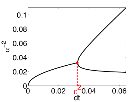
which is based on completing the square, and lagging linear terms which are incorporated into f~~𝑓\tilde{f}. In this case, we convolve twice with the Green’s function eα|x|superscript𝑒𝛼𝑥e^{-\alpha|x|}, where α=1ϵΔt𝛼1italic-ϵΔ𝑡\alpha=\frac{1}{\epsilon\sqrt{\Delta t}}. This switching is summarized by the bifurcation diagram shown in Figure 1.
Refer to caption
Figure 1. Bifurcation of the parameter 1α21superscript𝛼2\dfrac{1}{\alpha^{2}} in the modified Helmholtz operator \mathcal{L}.

Since both equations (16) and (17) converge to (8) as the iterations k𝑘k\to\infty, the overall scheme will be gradient stable. Thus, we invert the operator based on the parameters ΔtΔ𝑡\Delta t and ϵitalic-ϵ\epsilon as follows:

Factorization method(Δtϵ2)::Factorization methodΔ𝑡superscriptitalic-ϵ2absent\displaystyle\text{Factorization method}(\Delta t\geq\epsilon^{2}):\quad Invert (Ixxα12)(Ixxα22)Invert 𝐼subscript𝑥𝑥superscriptsubscript𝛼12𝐼subscript𝑥𝑥superscriptsubscript𝛼22\displaystyle\text{Invert }\left(I-\frac{\partial_{xx}}{\alpha_{1}^{2}}\right)\left(I-\frac{\partial_{xx}}{\alpha_{2}^{2}}\right)
Completed square method (Δt<ϵ2)::Completed square method Δ𝑡superscriptitalic-ϵ2absent\displaystyle\text{Completed square method }(\Delta t<\epsilon^{2}):\quad Invert (Ixxα2)2.Invert superscript𝐼subscript𝑥𝑥superscript𝛼22\displaystyle\text{Invert }\left(I-\frac{\partial_{xx}}{\alpha^{2}}\right)^{2}.
Remark 2.

The second iterative scheme (17) can be equivalently viewed as introducing a term of the form Sxx(vn+1,k+1vn+1,k)𝑆subscript𝑥𝑥superscript𝑣𝑛1𝑘1superscript𝑣𝑛1𝑘S\partial_{xx}(v^{n+1,k+1}-v^{n+1,k}) into the first (16), with S=2ϵ2Δt𝑆2superscriptitalic-ϵ2Δ𝑡S=2\sqrt{\epsilon^{2}\Delta t}. Numerical results confirm that both regimes, namely Δt<ϵ2Δ𝑡superscriptitalic-ϵ2\Delta t<\epsilon^{2} and Δ>ϵ2Δsuperscriptitalic-ϵ2\Delta>\epsilon^{2}, exhibit gradient stability.

Both iteration schemes require two inversions of a modified Helmholtz operator in [6], hence

=Ixxα2,𝐼subscript𝑥𝑥superscript𝛼2\mathcal{L}=I-\frac{\partial_{xx}}{\alpha^{2}}, (18)

with the different values of α𝛼\alpha. As we have indicated above, formal inversion of this operator [6] yields:

1[v](x)=[v](x)Particular Solution+Baeα(xa)+Bbeα(bx)Homogeneous Solution,axb,formulae-sequencesuperscript1delimited-[]𝑣𝑥subscriptdelimited-[]𝑣𝑥Particular Solutionsubscriptsubscript𝐵𝑎superscript𝑒𝛼𝑥𝑎subscript𝐵𝑏superscript𝑒𝛼𝑏𝑥Homogeneous Solution𝑎𝑥𝑏\mathcal{L}^{-1}[v](x)=\underbrace{\mathcal{I}[v](x)}_{\text{Particular Solution}}+\underbrace{\vphantom{I_{x}[u](x)}B_{a}e^{-\alpha(x-a)}+B_{b}e^{-\alpha(b-x)}}_{\text{Homogeneous Solution}},\quad a\leq x\leq b,

where the particular solution is a convolution with the Green’s function,

[v](x)=α2abeα|xx|v(x)𝑑x,delimited-[]𝑣𝑥𝛼2superscriptsubscript𝑎𝑏superscript𝑒𝛼𝑥superscript𝑥𝑣superscript𝑥differential-dsuperscript𝑥\mathcal{I}[v](x)=\frac{\alpha}{2}\int_{a}^{b}e^{-\alpha|x-x^{\prime}|}v(x^{\prime})dx^{\prime}, (19)

and the coefficients Basubscript𝐵𝑎B_{a} and Bbsubscript𝐵𝑏B_{b} are determined by applying boundary conditions at x=a,b𝑥𝑎𝑏x=a,b in Section 3.2.

Remark 3.

We observe that the Green’s function will be convolved with terms of the form xxfsubscript𝑥𝑥𝑓\partial_{xx}f, and so we will use the following result below

xx=α2(I)1[xxv]=α2(1I)[v],formulae-sequencesubscript𝑥𝑥superscript𝛼2𝐼superscript1delimited-[]subscript𝑥𝑥𝑣superscript𝛼2superscript1𝐼delimited-[]𝑣\partial_{xx}=\alpha^{2}(I-\mathcal{L})\quad\Longrightarrow\quad\mathcal{L}^{-1}[\partial_{xx}v]=\alpha^{2}\left(\mathcal{L}^{-1}-I\right)[v],

where we use the definition (18) of the modified Helmholtz operator \mathcal{L}.

3.2. Fully-discrete solution to 1D CH equation

It remains to discretize the convolution integral (18), and obtain a fully discrete algorithm. In our previous works [4, 7, 5, 6], we accomplish this with fast convolution; for convenience, we will summarize the fast algorithm here.

First, the particular solution (19) is split into [v](x)=L(x)+R(x)delimited-[]𝑣𝑥superscript𝐿𝑥superscript𝑅𝑥\mathcal{I}[v](x)=\mathcal{I}^{L}(x)+\mathcal{I}^{R}(x), where

L(x)=α2axeα(xx)v(x)𝑑x,R(x)=α2xbeα(xx)v(x)𝑑x.formulae-sequencesuperscript𝐿𝑥𝛼2superscriptsubscript𝑎𝑥superscript𝑒𝛼𝑥superscript𝑥𝑣superscript𝑥differential-dsuperscript𝑥superscript𝑅𝑥𝛼2superscriptsubscript𝑥𝑏superscript𝑒𝛼superscript𝑥𝑥𝑣superscript𝑥differential-dsuperscript𝑥\mathcal{I}^{L}(x)=\frac{\alpha}{2}\int_{a}^{x}e^{-\alpha(x-x^{\prime})}v(x^{\prime})dx^{\prime},\quad\mathcal{I}^{R}(x)=\frac{\alpha}{2}\int_{x}^{b}e^{-\alpha(x^{\prime}-x)}v(x^{\prime})dx^{\prime}.

The domain Ω[a,b]Ω𝑎𝑏\Omega\equiv[a,b] is partitioned into N𝑁N subdomains [xj1,xj]subscript𝑥𝑗1subscript𝑥𝑗[x_{j-1},x_{j}]

a=x0<x1<<xN=b,hj=xjxj1,formulae-sequence𝑎subscript𝑥0subscript𝑥1subscript𝑥𝑁𝑏subscript𝑗subscript𝑥𝑗subscript𝑥𝑗1a=x_{0}<x_{1}<\cdots<x_{N}=b,\quad h_{j}=x_{j}-x_{j-1},

we then evaluate the convolution operator at each grid point through j[v](xj)=jL+jRsubscript𝑗delimited-[]𝑣subscript𝑥𝑗subscriptsuperscript𝐿𝑗subscriptsuperscript𝑅𝑗\mathcal{I}_{j}\equiv\mathcal{I}[v](x_{j})=\mathcal{I}^{L}_{j}+\mathcal{I}^{R}_{j}. Since each integral satisfies exponential recursion [7, 5, 6],

jLsubscriptsuperscript𝐿𝑗\displaystyle\mathcal{I}^{L}_{j} =eαhjj1L+𝒥jL,𝒥jL=α2xj1xjeα(xjx)v(x)𝑑x,formulae-sequenceabsentsuperscript𝑒𝛼subscript𝑗subscriptsuperscript𝐿𝑗1subscriptsuperscript𝒥𝐿𝑗subscriptsuperscript𝒥𝐿𝑗𝛼2superscriptsubscriptsubscript𝑥𝑗1subscript𝑥𝑗superscript𝑒𝛼subscript𝑥𝑗superscript𝑥𝑣superscript𝑥differential-dsuperscript𝑥\displaystyle=e^{-\alpha h_{j}}\mathcal{I}^{L}_{j-1}+\mathcal{J}^{L}_{j},\quad\mathcal{J}^{L}_{j}=\frac{\alpha}{2}\int_{x_{j-1}}^{x_{j}}e^{-\alpha(x_{j}-x^{\prime})}v(x^{\prime})dx^{\prime}, (20)
jRsubscriptsuperscript𝑅𝑗\displaystyle\mathcal{I}^{R}_{j} =eαhj+1j+1R+𝒥jR,𝒥jR=α2xjxj+1eα(xxj)v(x)𝑑x.formulae-sequenceabsentsuperscript𝑒𝛼subscript𝑗1subscriptsuperscript𝑅𝑗1subscriptsuperscript𝒥𝑅𝑗subscriptsuperscript𝒥𝑅𝑗𝛼2superscriptsubscriptsubscript𝑥𝑗subscript𝑥𝑗1superscript𝑒𝛼superscript𝑥subscript𝑥𝑗𝑣superscript𝑥differential-dsuperscript𝑥\displaystyle=e^{-\alpha h_{j+1}}\mathcal{I}^{R}_{j+1}+\mathcal{J}^{R}_{j},\quad\mathcal{J}^{R}_{j}=\frac{\alpha}{2}\int_{x_{j}}^{x_{j+1}}e^{-\alpha(x^{\prime}-x_{j})}v(x^{\prime})dx^{\prime}. (21)

Those recursive updates are still exact, and only require computing the "local" convolutions 𝒥jLsuperscriptsubscript𝒥𝑗𝐿\mathcal{J}_{j}^{L} and 𝒥jRsuperscriptsubscript𝒥𝑗𝑅\mathcal{J}_{j}^{R}. In [6], we derived a spatial quadrature of general order M2𝑀2M\geq 2 for computing these local integrals. For example, the second-order accurate (M=2)𝑀2(M=2) quadrature on a uniform grid (hj=Δx)subscript𝑗Δ𝑥(h_{j}=\Delta x) is given by

JjLsubscriptsuperscript𝐽𝐿𝑗\displaystyle J^{L}_{j} Pv(xj)+Qv(xj1)+R(v(xj+1)2v(xj)+v(xj1))absent𝑃𝑣subscript𝑥𝑗𝑄𝑣subscript𝑥𝑗1𝑅𝑣subscript𝑥𝑗12𝑣subscript𝑥𝑗𝑣subscript𝑥𝑗1\displaystyle\approx Pv(x_{j})+Qv(x_{j-1})+R(v(x_{j+1})-2v(x_{j})+v(x_{j-1})) (22)
JjRsubscriptsuperscript𝐽𝑅𝑗\displaystyle J^{R}_{j} Pv(xj)+Qv(xj+1)+R(v(xj+1)2v(xj)+v(xj1))absent𝑃𝑣subscript𝑥𝑗𝑄𝑣subscript𝑥𝑗1𝑅𝑣subscript𝑥𝑗12𝑣subscript𝑥𝑗𝑣subscript𝑥𝑗1\displaystyle\approx Pv(x_{j})+Qv(x_{j+1})+R(v(x_{j+1})-2v(x_{j})+v(x_{j-1})) (23)

where defining ν=αΔx𝜈𝛼Δ𝑥\nu=\alpha\Delta x and d=eν𝑑superscript𝑒𝜈d=e^{-\nu}, the quadrature weights are given by

P𝑃\displaystyle P =11dν,absent11𝑑𝜈\displaystyle=1-\frac{1-d}{\nu},
Q𝑄\displaystyle Q =d+1dν,absent𝑑1𝑑𝜈\displaystyle=-d+\frac{1-d}{\nu},
R𝑅\displaystyle R =1dν21+d2ν.absent1𝑑superscript𝜈21𝑑2𝜈\displaystyle=\frac{1-d}{\nu^{2}}-\frac{1+d}{2\nu}.

Likewise, for higher order methods (M>2𝑀2M>2), the quadrature weights are pre-computed, so that the fast convolution algorithm is achieved as 𝒪(MN)𝒪𝑀𝑁\mathcal{O}(MN) per time step with user-defined order M𝑀M in space. In every simulation in this work, we choose M=4𝑀4M=4 or M=6𝑀6M=6.

Next, the homogeneous solution (18) is used to enforce various boundary conditions. For example periodic boundary conditions lead to

vn(a)=vn(b),vxn(a)=vxn(b),n.formulae-sequencesuperscript𝑣𝑛𝑎superscript𝑣𝑛𝑏formulae-sequencesuperscriptsubscript𝑣𝑥𝑛𝑎superscriptsubscript𝑣𝑥𝑛𝑏for-all𝑛v^{n}(a)=v^{n}(b),\quad v_{x}^{n}(a)=v_{x}^{n}(b),\quad\forall n\in\mathbb{N}.

and evaluation of (18) at x=a,b𝑥𝑎𝑏x=a,b, produces a 2×2222\times 2 system for the unknowns Basubscript𝐵𝑎B_{a} and Bbsubscript𝐵𝑏B_{b}:

1[vn](a)=1[vn](b)superscript1delimited-[]superscript𝑣𝑛𝑎superscript1delimited-[]superscript𝑣𝑛𝑏\displaystyle\mathcal{L}^{-1}[v^{n}](a)=\mathcal{L}^{-1}[v^{n}](b)\quad 0+Ba+Bbμ=N+Baμ+Bb,subscript0subscript𝐵𝑎subscript𝐵𝑏𝜇subscript𝑁subscript𝐵𝑎𝜇subscript𝐵𝑏\displaystyle\Longleftrightarrow\quad\mathcal{I}_{0}+B_{a}+B_{b}\mu=\mathcal{I}_{N}+B_{a}\mu+B_{b},
x1[vn](a)=x1[vn](b)superscriptsubscript𝑥1delimited-[]superscript𝑣𝑛𝑎superscriptsubscript𝑥1delimited-[]superscript𝑣𝑛𝑏\displaystyle\mathcal{L}_{x}^{-1}[v^{n}](a)=\mathcal{L}_{x}^{-1}[v^{n}](b)\quad α(0Ba+Bbμ)=α(N+Baμ+Bb).𝛼subscript0subscript𝐵𝑎subscript𝐵𝑏𝜇𝛼subscript𝑁subscript𝐵𝑎𝜇subscript𝐵𝑏\displaystyle\Longleftrightarrow\quad\alpha(\mathcal{I}_{0}-B_{a}+B_{b}\mu)=\alpha(-\mathcal{I}_{N}+B_{a}\mu+B_{b}).

Solving this linear system yields

Ba=N1μ,Bb=01μ,formulae-sequencesubscript𝐵𝑎subscript𝑁1𝜇subscript𝐵𝑏subscript01𝜇B_{a}=\frac{\mathcal{I}_{N}}{1-\mu},\quad B_{b}=\frac{\mathcal{I}_{0}}{1-\mu}, (24)

where μ=eα(ba)𝜇superscript𝑒𝛼𝑏𝑎\mu=e^{-\alpha(b-a)} and 0=[v](a)subscript0delimited-[]𝑣𝑎\mathcal{I}_{0}=\mathcal{I}[v](a) and N=[v](b)subscript𝑁delimited-[]𝑣𝑏\mathcal{I}_{N}=\mathcal{I}[v](b). Other boundary conditions (e.g. Neumann, Dirichlet) follow the analogous procedure that requires solving a simple 2×2222\times 2 linear system. (cf. [5])

4. Higher order schemes

In this Section we formulate second and third order time accurate methods by combining the ideas of MOLTT{}^{\text{T}} formulation with backward difference formulas (BDF), singly diagonal implicit Runge-Kutta (SDIRK), and spectral deferred correction (SDC) methods. We will present several refinement studies to compare these approaches.

4.1. MOLTT{}^{\text{T}} with BDF

The BDF time stepping methods are one of the most commonly used implicit linear multi-step methods [16]. To achieve the desired order of accuracy, we discretize the time derivative using BDF formulas as follows:

BDF2: (I+23ϵ2Δtxxxx)vn+1=43vn13vn1+23Δtxxfn+1,𝐼23superscriptitalic-ϵ2Δ𝑡subscript𝑥𝑥𝑥𝑥superscript𝑣𝑛143superscript𝑣𝑛13superscript𝑣𝑛123Δ𝑡subscript𝑥𝑥superscript𝑓𝑛1\displaystyle\left(I+\frac{2}{3}\epsilon^{2}\Delta t\partial_{xxxx}\right)v^{n+1}=\frac{4}{3}v^{n}-\frac{1}{3}v^{n-1}+\frac{2}{3}\Delta t\partial_{xx}f^{n+1}, (25)
BDF3: (I+611ϵ2Δtxxxx)vn+1=1811vn911vn1+211vn2+611Δtxxfn+1,𝐼611superscriptitalic-ϵ2Δ𝑡subscript𝑥𝑥𝑥𝑥superscript𝑣𝑛11811superscript𝑣𝑛911superscript𝑣𝑛1211superscript𝑣𝑛2611Δ𝑡subscript𝑥𝑥superscript𝑓𝑛1\displaystyle\left(I+\frac{6}{11}\epsilon^{2}\Delta t\partial_{xxxx}\right)v^{n+1}=\frac{18}{11}v^{n}-\frac{9}{11}v^{n-1}+\frac{2}{11}v^{n-2}+\frac{6}{11}\Delta t\partial_{xx}f^{n+1}, (26)

where we now require two and three previous time steps, respectively. Similar to the first-order scheme in Section 3.1, we define two fixed-point iterations, depending on the time step ΔtΔ𝑡\Delta t. First, energy-stable factorization iteration which has a time step lower bound for real-valued Green’s functions. Second, completed square version by adding S(vn+1,k+1vn+1,k)𝑆superscript𝑣𝑛1𝑘1superscript𝑣𝑛1𝑘S(v^{n+1,k+1}-v^{n+1,k}) term, which has a time step upper bound for energy stability. Specifically, the BDF 2 formulation (25) utilizes

Δt32ϵ2::Δ𝑡32superscriptitalic-ϵ2absent\displaystyle\Delta t\geq\frac{3}{2}\epsilon^{2}:\quad =I43Δtxx+23ϵ2Δtxxxx=(Ixxα12)(Ixxα22),𝐼43Δ𝑡subscript𝑥𝑥23superscriptitalic-ϵ2Δ𝑡subscript𝑥𝑥𝑥𝑥𝐼subscript𝑥𝑥superscriptsubscript𝛼12𝐼subscript𝑥𝑥superscriptsubscript𝛼22\displaystyle\mathcal{L}=I-\frac{4}{3}\Delta t\partial_{xx}+\frac{2}{3}\epsilon^{2}\Delta t\partial_{xxxx}=\left(I-\frac{\partial_{xx}}{\alpha_{1}^{2}}\right)\left(I-\frac{\partial_{xx}}{\alpha_{2}^{2}}\right),
Δt<32ϵ2::Δ𝑡32superscriptitalic-ϵ2absent\displaystyle\Delta t<\frac{3}{2}\epsilon^{2}:\quad =I223ϵ2Δtxx+23ϵ2Δtxxxx=(Ixxα2)2,𝐼223superscriptitalic-ϵ2Δ𝑡subscript𝑥𝑥23superscriptitalic-ϵ2Δ𝑡subscript𝑥𝑥𝑥𝑥superscript𝐼subscript𝑥𝑥superscript𝛼22\displaystyle\mathcal{L}=I-2\sqrt{\frac{2}{3}\epsilon^{2}\Delta t}\partial_{xx}+\frac{2}{3}\epsilon^{2}\Delta t\partial_{xxxx}=\left(I-\frac{\partial_{xx}}{\alpha^{2}}\right)^{2},

where

1α12=23Δt+(23Δt)223ϵ2Δt,1α22=23Δt(23Δt)223ϵ2Δt,1α2=23ϵ2Δt.formulae-sequence1superscriptsubscript𝛼1223Δ𝑡superscript23Δ𝑡223superscriptitalic-ϵ2Δ𝑡formulae-sequence1superscriptsubscript𝛼2223Δ𝑡superscript23Δ𝑡223superscriptitalic-ϵ2Δ𝑡1superscript𝛼223superscriptitalic-ϵ2Δ𝑡\frac{1}{\alpha_{1}^{2}}=\frac{2}{3}\Delta t+\sqrt{\left(\frac{2}{3}\Delta t\right)^{2}-\frac{2}{3}\epsilon^{2}\Delta t},\quad\frac{1}{\alpha_{2}^{2}}=\frac{2}{3}\Delta t-\sqrt{\left(\frac{2}{3}\Delta t\right)^{2}-\frac{2}{3}\epsilon^{2}\Delta t},\quad\frac{1}{\alpha^{2}}=\sqrt{\frac{2}{3}\epsilon^{2}\Delta t}.

A similar result is obtained for the BDF 3 method. The main advantage of BDF schemes is that the extension of first-order methods to higher-order is very straightforward. However, they also require initialization of the first few time steps. In next section, we will look at Ruge-Kutta (RK) methods, which do not have this requirement.

4.2. MOLTT{}^{\text{T}} with SDIRK

Singly implicit RK methods (SDIRK) are those which have the same diagonal elements in the Butcher Table, [1]. To obtain a Pthsuperscript𝑃tP^{\text{t}h} order method, RK methods, P𝑃P intermediate steps are computed at each time step. The second order method, SDIRK2, is as follows

(I+ηϵ2Δtxxxx)K1𝐼𝜂superscriptitalic-ϵ2Δ𝑡subscript𝑥𝑥𝑥𝑥subscript𝐾1\displaystyle\left(I+\eta\epsilon^{2}\Delta t\partial_{xxxx}\right)K_{1} =ϵ2xxxxvn+xxf(vn+ηΔtK1),η=122,formulae-sequenceabsentsuperscriptitalic-ϵ2subscript𝑥𝑥𝑥𝑥superscript𝑣𝑛subscript𝑥𝑥𝑓superscript𝑣𝑛𝜂Δ𝑡subscript𝐾1𝜂122\displaystyle=-\epsilon^{2}\partial_{xxxx}v^{n}+\partial_{xx}f\left(v^{n}+\eta\Delta tK_{1}\right),\quad\eta=1-\frac{\sqrt{2}}{2},
(I+ηϵ2Δtxxxx)K2𝐼𝜂superscriptitalic-ϵ2Δ𝑡subscript𝑥𝑥𝑥𝑥subscript𝐾2\displaystyle\left(I+\eta\epsilon^{2}\Delta t\partial_{xxxx}\right)K_{2} =ϵ2xxxx(vn+(1η)ΔtK1)+xxf(vn+(1η)ΔtK1+ηΔtK2)absentsuperscriptitalic-ϵ2subscript𝑥𝑥𝑥𝑥superscript𝑣𝑛1𝜂Δ𝑡subscript𝐾1subscript𝑥𝑥𝑓superscript𝑣𝑛1𝜂Δ𝑡subscript𝐾1𝜂Δ𝑡subscript𝐾2\displaystyle=-\epsilon^{2}\partial_{xxxx}\left(v^{n}+(1-\eta)\Delta tK_{1}\right)+\partial_{xx}f\left(v^{n}+(1-\eta)\Delta tK_{1}+\eta\Delta tK_{2}\right)
vn+1superscript𝑣𝑛1\displaystyle v^{n+1} =vn+Δt{(1η)K1+ηK2},absentsuperscript𝑣𝑛Δ𝑡1𝜂subscript𝐾1𝜂subscript𝐾2\displaystyle=v^{n}+\Delta t\{(1-\eta)K_{1}+\eta K_{2}\},

where η𝜂\eta is the root of the polynomial 122η+η2122𝜂superscript𝜂2\frac{1}{2}-2\eta+\eta^{2}, as derived from the order conditions [1]. Next, we construct two intermediate solution K1subscript𝐾1K_{1} and K2subscript𝐾2K_{2}, using nonlinear iterative schemes based on Section 4.1. First, if Δtϵ2ηΔ𝑡superscriptitalic-ϵ2𝜂\Delta t\geq\dfrac{\epsilon^{2}}{\eta},

K1n+1,k+1superscriptsubscript𝐾1𝑛1𝑘1\displaystyle K_{1}^{n+1,k+1} =1121[ϵ2xxxxvn+xx(f~(vn+ηΔtK1n+1,k)+2vn)],i=Ixxαi2formulae-sequenceabsentsuperscriptsubscript11superscriptsubscript21delimited-[]superscriptitalic-ϵ2subscript𝑥𝑥𝑥𝑥superscript𝑣𝑛subscript𝑥𝑥~𝑓superscript𝑣𝑛𝜂Δ𝑡superscriptsubscript𝐾1𝑛1𝑘2superscript𝑣𝑛subscript𝑖𝐼subscript𝑥𝑥superscriptsubscript𝛼𝑖2\displaystyle=\mathcal{L}_{1}^{-1}\mathcal{L}_{2}^{-1}\left[-\epsilon^{2}\partial_{xxxx}v^{n}+\partial_{xx}\left(\tilde{f}\left(v^{n}+\eta\Delta tK_{1}^{n+1,k}\right)+2v^{n}\right)\right],\quad\mathcal{L}_{i}=I-\frac{\partial_{xx}}{\alpha_{i}^{2}}
K2n+1,k+1superscriptsubscript𝐾2𝑛1𝑘1\displaystyle K_{2}^{n+1,k+1} =1121[ϵ2xxxx(vn+(1η)ΔtK1n+1,k)\displaystyle=\mathcal{L}_{1}^{-1}\mathcal{L}_{2}^{-1}\biggl{[}-\epsilon^{2}\partial_{xxxx}\left(v^{n}+(1-\eta)\Delta tK_{1}^{n+1,k}\right)
+\displaystyle+ xx(f~(vn+(1η)ΔtK1n+1,k+ηΔtK2n+1,k)+2(vn+(1η)ΔtK1n+1,k))],\displaystyle\partial_{xx}\left(\tilde{f}\left(v^{n}+(1-\eta)\Delta tK_{1}^{n+1,k}+\eta\Delta tK_{2}^{n+1,k}\right)+2(v^{n}+(1-\eta)\Delta tK_{1}^{n+1,k})\right)\biggr{]},

where 1α12=ηΔt+(ηΔt)2ϵ2ηΔt1superscriptsubscript𝛼12𝜂Δ𝑡superscript𝜂Δ𝑡2superscriptitalic-ϵ2𝜂Δ𝑡\dfrac{1}{\alpha_{1}^{2}}=\eta\Delta t+\sqrt{(\eta\Delta t)^{2}-\epsilon^{2}\eta\Delta t} and 1α22=ηΔt(ηΔt)2ϵ2ηΔt1superscriptsubscript𝛼22𝜂Δ𝑡superscript𝜂Δ𝑡2superscriptitalic-ϵ2𝜂Δ𝑡\dfrac{1}{\alpha_{2}^{2}}=\eta\Delta t-\sqrt{(\eta\Delta t)^{2}-\epsilon^{2}\eta\Delta t}. If Δt<ϵ2ηΔ𝑡superscriptitalic-ϵ2𝜂\Delta t<\dfrac{\epsilon^{2}}{\eta},

K1n+1,k+1superscriptsubscript𝐾1𝑛1𝑘1\displaystyle K_{1}^{n+1,k+1} =2[ϵ2xxxxvn+xx(f(vn+ηΔtK1n+1,k)2ηϵ2ΔtK1n+1,k)],absentsuperscript2delimited-[]superscriptitalic-ϵ2subscript𝑥𝑥𝑥𝑥superscript𝑣𝑛subscript𝑥𝑥𝑓superscript𝑣𝑛𝜂Δ𝑡superscriptsubscript𝐾1𝑛1𝑘2𝜂superscriptitalic-ϵ2Δ𝑡superscriptsubscript𝐾1𝑛1𝑘\displaystyle=\mathcal{L}^{-2}\left[-\epsilon^{2}\partial_{xxxx}v^{n}+\partial_{xx}\left(f\left(v^{n}+\eta\Delta tK_{1}^{n+1,k}\right)-2\sqrt{\eta\epsilon^{2}\Delta t}K_{1}^{n+1,k}\right)\right],
K2n+1,k+1superscriptsubscript𝐾2𝑛1𝑘1\displaystyle K_{2}^{n+1,k+1} =2[ϵ2xxxx(vn+(1η)ΔtK1n+1,k)\displaystyle=\mathcal{L}^{-2}\biggl{[}-\epsilon^{2}\partial_{xxxx}\left(v^{n}+(1-\eta)\Delta tK_{1}^{n+1,k}\right)
+xx(f(vn+(1η)ΔtK1n+1,k+ηΔtK2n+1,k)2ηϵ2ΔtK2n+1,k)],\displaystyle+\partial_{xx}\left(f\left(v^{n}+(1-\eta)\Delta tK_{1}^{n+1,k}+\eta\Delta tK_{2}^{n+1,k}\right)-2\sqrt{\eta\epsilon^{2}\Delta t}K_{2}^{n+1,k}\right)\biggr{]},

where Iηϵ2Δtxx𝐼𝜂superscriptitalic-ϵ2Δ𝑡subscript𝑥𝑥\mathcal{L}\equiv I-\sqrt{\eta\epsilon^{2}\Delta t}\partial_{xx} is used. Below we will also make use of SDIRK3, which can be derived in a similar fashion.

Remark 4.

Similar to Remark 3, the fourth derivative can be calculated as follows,

xxxx=α12α22(I1)(I2)1121[xxxxv]=α12α22(11I)(21I)[v].formulae-sequencesubscript𝑥𝑥𝑥𝑥superscriptsubscript𝛼12superscriptsubscript𝛼22𝐼subscript1𝐼subscript2superscriptsubscript11superscriptsubscript21delimited-[]subscript𝑥𝑥𝑥𝑥𝑣superscriptsubscript𝛼12superscriptsubscript𝛼22superscriptsubscript11𝐼superscriptsubscript21𝐼delimited-[]𝑣\partial_{xxxx}=\alpha_{1}^{2}\alpha_{2}^{2}(I-\mathcal{L}_{1})(I-\mathcal{L}_{2})\quad\Longrightarrow\quad\mathcal{L}_{1}^{-1}\mathcal{L}_{2}^{-1}[\partial_{xxxx}v]=\alpha_{1}^{2}\alpha_{2}^{2}\left(\mathcal{L}_{1}^{-1}-I\right)\left(\mathcal{L}_{2}^{-1}-I\right)[v].

In Section 4.4 we will present refinement studies for both the BDF and SDIRK methods. We note that for a small enough time step ΔtΔ𝑡\Delta t, both methods converge as expected. However for the corresponding third-order methods (BDF3 and SDIRK3), as ΔtΔ𝑡\Delta t increases the order of convergence begins to plateau. To resolve this issue, we will suggest another higher order method.

4.3. MOLTT{}^{\text{T}} with SDC

The spectral deferred correction (SDC) methods are a class of time integrators [13]. First a prediction to the solution ("level 0") is computed using low order schemes (e.g. Backward Euler), and then the error (defect) is corrected at subsequent stages, using higher order integrators. Our SDC procedure follows the presentation in [10].

  1. (1)

    Prediction step (level [0]): Subdivide the time interval [0,T]0𝑇[0,T] with uniform ΔtΔ𝑡\Delta t:

    0t0<t1<<tNtT.0superscript𝑡0superscript𝑡1superscript𝑡subscript𝑁𝑡𝑇0\equiv t^{0}<t^{1}<\cdots<t^{N_{t}}\equiv T.

    Compute {vm[0](x)}0mNtsubscriptsubscriptsuperscript𝑣delimited-[]0𝑚𝑥0𝑚subscript𝑁𝑡\{v^{[0]}_{m}(x)\}_{0\leq m\leq N_{t}} via Backward Euler approximation in (8) for CH equation, which is first-order approximation to the exact solution {ym(x)}0mNtsubscriptsubscript𝑦𝑚𝑥0𝑚subscript𝑁𝑡\{y_{m}(x)\}_{0\leq m\leq N_{t}}.

  2. (2)

    Correction step (level [1]): Assume that v(0)(x,t)superscript𝑣0𝑥𝑡v^{(0)}(x,t) is a polynomial interpolant, approximating the exact solution y(x,t)𝑦𝑥𝑡y(x,t) satisfying

    v(0)(x,tm)vm[0](x),m=n+1,n,,n+1P,formulae-sequencesuperscript𝑣0𝑥superscript𝑡𝑚subscriptsuperscript𝑣delimited-[]0𝑚𝑥𝑚𝑛1𝑛𝑛1𝑃v^{(0)}(x,t^{m})\equiv v^{[0]}_{m}(x),\quad m=n+1,n,\cdots,n+1-P,

    where P𝑃P will be specified later. The error equation is defined

    e(x,t)=y(x,t)v(0)(x,t),𝑒𝑥𝑡𝑦𝑥𝑡superscript𝑣0𝑥𝑡e(x,t)=y(x,t)-v^{(0)}(x,t),

    and the residual (or "defect") is

    γ(x,t)=vt(0)CH(v(0)),CH(v)=ϵ2xxxxv+xxf(v).formulae-sequence𝛾𝑥𝑡subscriptsuperscript𝑣0𝑡subscriptCHsuperscript𝑣0subscriptCH𝑣superscriptitalic-ϵ2subscript𝑥𝑥𝑥𝑥𝑣subscript𝑥𝑥𝑓𝑣\gamma(x,t)=v^{(0)}_{t}-\mathcal{F}_{\text{CH}}(v^{(0)}),\quad\mathcal{F}_{\text{CH}}(v)=-\epsilon^{2}\partial_{xxxx}v+\partial_{xx}f(v).

    We take the derivative of the error equation with respect to t𝑡t, and rewrite it using the residual definition,

    et(x,t)=yt(x,t)vt(0)(x,t)CH(y(x,t))CH(v(0)(x,t))γ(x,t),subscript𝑒𝑡𝑥𝑡subscript𝑦𝑡𝑥𝑡subscriptsuperscript𝑣0𝑡𝑥𝑡subscriptCH𝑦𝑥𝑡subscriptCHsuperscript𝑣0𝑥𝑡𝛾𝑥𝑡\displaystyle\quad e_{t}(x,t)=y_{t}(x,t)-v^{(0)}_{t}(x,t)\equiv\mathcal{F}_{\text{CH}}(y(x,t))-\mathcal{F}_{\text{CH}}(v^{(0)}(x,t))-\gamma(x,t),
    \displaystyle\Longleftrightarrow et(x,t)+γ(x,t)=CH((e+v(0))(x,t))CH(v(0)(x,t)),subscript𝑒𝑡𝑥𝑡𝛾𝑥𝑡subscriptCH𝑒superscript𝑣0𝑥𝑡subscriptCHsuperscript𝑣0𝑥𝑡\displaystyle\quad e_{t}(x,t)+\gamma(x,t)=\mathcal{F}_{\text{CH}}((e+v^{(0)})(x,t))-\mathcal{F}_{\text{CH}}(v^{(0)}(x,t)),
    \displaystyle\Longleftrightarrow t(v(1)(x,t)0tCH(v(0)(x,τ))𝑑τ)=CH(v(1)(x,t))CH(v(0)(x,t)),𝑡superscript𝑣1𝑥𝑡superscriptsubscript0𝑡subscriptCHsuperscript𝑣0𝑥𝜏differential-d𝜏subscriptCHsuperscript𝑣1𝑥𝑡subscriptCHsuperscript𝑣0𝑥𝑡\displaystyle\quad\frac{\partial}{\partial t}\left(v^{(1)}(x,t)-\int_{0}^{t}\mathcal{F}_{\text{CH}}(v^{(0)}(x,\tau))d\tau\right)=\mathcal{F}_{\text{CH}}(v^{(1)}(x,t))-\mathcal{F}_{\text{CH}}(v^{(0)}(x,t)),

    where we assume that the initial condition e(x,0)=0𝑒𝑥00e(x,0)=0, and v(1)=v(0)+esuperscript𝑣1superscript𝑣0𝑒v^{(1)}=v^{(0)}+e. Hence, our updating "level [1]" solution {vm[1]}subscriptsuperscript𝑣delimited-[]1𝑚\{v^{[1]}_{m}\} is found by approximating the above differential equation with the same method as "level 0". We apply the backward Euler scheme, thus

    vn+1[1]vn[1]=Δt(CH(vn+1[1])CH(vn+1[0]))+tntn+1CH(v(0)(x,τ))𝑑τ.subscriptsuperscript𝑣delimited-[]1𝑛1subscriptsuperscript𝑣delimited-[]1𝑛Δ𝑡subscriptCHsubscriptsuperscript𝑣delimited-[]1𝑛1subscriptCHsubscriptsuperscript𝑣delimited-[]0𝑛1superscriptsubscriptsuperscript𝑡𝑛superscript𝑡𝑛1subscriptCHsuperscript𝑣0𝑥𝜏differential-d𝜏v^{[1]}_{n+1}-v^{[1]}_{n}=\Delta t\left(\mathcal{F}_{\text{CH}}(v^{[1]}_{n+1})-\mathcal{F}_{\text{CH}}(v^{[0]}_{n+1})\right)+\int_{t^{n}}^{t^{n+1}}\mathcal{F}_{\text{CH}}(v^{(0)}(x,\tau))d\tau. (27)
  3. (3)

    Correction step (level [j]): The process is then iterated by generalizing (27),

    vn+1[j]ΔtCH(vn+1[j])=vn[j]ΔtCH(vn+1[j1])+tntn+1CH(v(j1)(x,τ))𝑑τ,subscriptsuperscript𝑣delimited-[]𝑗𝑛1Δ𝑡subscriptCHsubscriptsuperscript𝑣delimited-[]𝑗𝑛1subscriptsuperscript𝑣delimited-[]𝑗𝑛Δ𝑡subscriptCHsubscriptsuperscript𝑣delimited-[]𝑗1𝑛1superscriptsubscriptsuperscript𝑡𝑛superscript𝑡𝑛1subscriptCHsuperscript𝑣𝑗1𝑥𝜏differential-d𝜏v^{[j]}_{n+1}-\Delta t\mathcal{F}_{\text{CH}}(v^{[j]}_{n+1})=v^{[j]}_{n}-\Delta t\mathcal{F}_{\text{CH}}(v^{[j-1]}_{n+1})+\int_{t^{n}}^{t^{n+1}}\mathcal{F}_{\text{CH}}(v^{(j-1)}(x,\tau))d\tau, (28)

    where the terms including updating solution v[j]superscript𝑣delimited-[]𝑗v^{[j]} have been collected on the left hand side, and the old solution v[j1]superscript𝑣delimited-[]𝑗1v^{[j-1]} are on the right hand side.

To complete SDC, we must consider an approximation of the integral in (28):

tntn+1CH(v(j1)(x,τ))𝑑τ={Δti=0Pq~in+1i[j1],ifnP1,Δti=0Pq~ii[j1]ifn<P1,superscriptsubscriptsuperscript𝑡𝑛superscript𝑡𝑛1subscriptCHsuperscript𝑣𝑗1𝑥𝜏differential-d𝜏casesΔ𝑡superscriptsubscript𝑖0𝑃subscript~𝑞𝑖subscriptsuperscriptdelimited-[]𝑗1𝑛1𝑖if𝑛𝑃1Δ𝑡superscriptsubscript𝑖0𝑃subscript~𝑞𝑖subscriptsuperscriptdelimited-[]𝑗1𝑖if𝑛𝑃1\int_{t^{n}}^{t^{n+1}}\mathcal{F}_{\text{CH}}(v^{(j-1)}(x,\tau))d\tau=\begin{cases}\Delta t\sum_{i=0}^{P}\tilde{q}_{i}\mathcal{F}^{[j-1]}_{n+1-i},\qquad&\text{if}\quad n\geq P-1,\\ \Delta t\sum_{i=0}^{P}\ \tilde{q}_{i}\mathcal{F}^{[j-1]}_{i}\qquad&\text{if}\quad n<P-1,\end{cases} (29)

where n[j1]=CH(vn[j1])subscriptsuperscriptdelimited-[]𝑗1𝑛subscriptCHsubscriptsuperscript𝑣delimited-[]𝑗1𝑛\mathcal{F}^{[j-1]}_{n}=\mathcal{F}_{\text{CH}}(v^{[j-1]}_{n}), and q~isubscript~𝑞𝑖\tilde{q}_{i} are quadrature weights (cf. [10]). Note that the number of terms in the sum (29) is P+1𝑃1P+1, where P𝑃P is the order of polynomial interpolation v(j1)superscript𝑣𝑗1v^{(j-1)}. The integral must be approximated with increasing accuracy as the level increases, so that Pj𝑃𝑗P\geq j at "level [j]delimited-[]𝑗[j]". In Section 4.4, we will show that this order P𝑃P affects the asymptotic region of stability of SDC3 method.

We now combine MOLTT{}^{\text{T}} scheme with these higher-order SDC methods. For instance, the second-order SDC scheme (SDC2) only requires one more correction (level [1]delimited-[]1[1]). If Δtϵ2Δ𝑡superscriptitalic-ϵ2\Delta t\geq\epsilon^{2},

vn+1,k+1[1]=1121[vn[1]+Δtxx(f~n+1,k[1]fn+1[0]fn[0]2)+ϵ2Δt2xxxx(vn+1[0]vn[0])]subscriptsuperscript𝑣delimited-[]1𝑛1𝑘1superscriptsubscript11superscriptsubscript21delimited-[]subscriptsuperscript𝑣delimited-[]1𝑛Δ𝑡subscript𝑥𝑥subscriptsuperscript~𝑓delimited-[]1𝑛1𝑘subscriptsuperscript𝑓delimited-[]0𝑛1subscriptsuperscript𝑓delimited-[]0𝑛2superscriptitalic-ϵ2Δ𝑡2subscript𝑥𝑥𝑥𝑥subscriptsuperscript𝑣delimited-[]0𝑛1subscriptsuperscript𝑣delimited-[]0𝑛\displaystyle v^{[1]}_{n+1,k+1}=\mathcal{L}_{1}^{-1}\mathcal{L}_{2}^{-1}\left[v^{[1]}_{n}+\Delta t\partial_{xx}\left(\tilde{f}^{[1]}_{n+1,k}-\frac{{f}^{[0]}_{n+1}-f^{[0]}_{n}}{2}\right)+\frac{\epsilon^{2}\Delta t}{2}\partial_{xxxx}\left(v^{[0]}_{n+1}-v^{[0]}_{n}\right)\right] (30)

where quadrature weights of (29) are q~1=q~2=12subscript~𝑞1subscript~𝑞212\tilde{q}_{1}=\tilde{q}_{2}=\frac{1}{2} (P=1𝑃1P=1: trapezoidal rule) and isubscript𝑖\mathcal{L}_{i} are same with the first-order scheme in Section 3.1. Similarly, if Δt<ϵ2,Δ𝑡superscriptitalic-ϵ2\Delta t<\epsilon^{2},

vn+1,k+1[1]=2[vn[1]+Δtxx(fn+1,k[1]2ϵ2Δtvn+1,k[1]fn+1[0]fn[0]2)+ϵ2Δt2xxxx(vn+1[0]vn[0])]subscriptsuperscript𝑣delimited-[]1𝑛1𝑘1superscript2delimited-[]subscriptsuperscript𝑣delimited-[]1𝑛Δ𝑡subscript𝑥𝑥subscriptsuperscript𝑓delimited-[]1𝑛1𝑘2superscriptitalic-ϵ2Δ𝑡subscriptsuperscript𝑣delimited-[]1𝑛1𝑘subscriptsuperscript𝑓delimited-[]0𝑛1subscriptsuperscript𝑓delimited-[]0𝑛2superscriptitalic-ϵ2Δ𝑡2subscript𝑥𝑥𝑥𝑥subscriptsuperscript𝑣delimited-[]0𝑛1subscriptsuperscript𝑣delimited-[]0𝑛\displaystyle v^{[1]}_{n+1,k+1}=\mathcal{L}^{-2}\left[v^{[1]}_{n}+\Delta t\partial_{xx}\left(f^{[1]}_{n+1,k}-2\sqrt{\frac{\epsilon^{2}}{\Delta t}}v^{[1]}_{n+1,k}-\frac{{f}^{[0]}_{n+1}-f^{[0]}_{n}}{2}\right)+\frac{\epsilon^{2}\Delta t}{2}\partial_{xxxx}\left(v^{[0]}_{n+1}-v^{[0]}_{n}\right)\right] (31)

4.4. Refinement studies for higher order methods

We solve (1) with periodic boundary conditions, with the same initial condition used in [9],

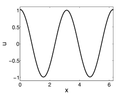
u0(x)=cos(2x)+1100ecos(x+110),x[0,2π].formulae-sequencesubscript𝑢0𝑥2𝑥1100superscript𝑒𝑥110𝑥02𝜋u_{0}(x)=\cos(2x)+\dfrac{1}{100}e^{\cos\left(x+\frac{1}{10}\right)},\qquad x\in[0,2\pi]. (32)

We integrate up to a final time Tfinalsubscript𝑇finalT_{\text{final}} using each second-order method. Since an exact solution is not available, we perform time refinement using successive approximations, and the approximate error with step size ΔtΔ𝑡\Delta t is uΔtuΔt/2subscriptnormsubscript𝑢Δ𝑡subscript𝑢Δ𝑡2\|u_{\Delta t}-u_{\Delta t/2}\|_{\infty}, measured in the maximum norm. Successive errors for each second-order method is presented in Table 1. The parameters used for all computations were:

ϵ=0.18,Δx=2π5120.0123,Tfinal=1,Ntol=1012,formulae-sequenceformulae-sequenceitalic-ϵ0.18Δ𝑥2𝜋5120.0123formulae-sequencesubscript𝑇final1subscript𝑁tolsuperscript1012\epsilon=0.18,\quad\Delta x=\dfrac{2\pi}{512}\approx 0.0123,\quad T_{\text{final}}=1,\quad N_{\text{tol}}=10^{-12}, (33)

where Ntolsubscript𝑁tolN_{\text{tol}} is a tolerance for fixed point iterations such that vn+1,k+1vn+1,k<Ntolsubscriptnormsuperscript𝑣𝑛1𝑘1superscript𝑣𝑛1𝑘subscript𝑁tol\|v^{n+1,k+1}-v^{n+1,k}\|_{\infty}<N_{\text{tol}}. We use 6thsuperscript6th6^{\text{th}}-order spatial quadrature, so that the dominant error was temporal.

Refer to caption
(a) Energy decay (2ndsuperscript2nd2^{\text{nd}} order methods)
Refer to caption
(b) Iteration count(2ndsuperscript2nd2^{\text{nd}} order methods)
Refer to caption
(c) Energy decay (3rdsuperscript3rd3^{\text{rd}} order methods)
Refer to caption
(d) Iteration count (3rdsuperscript3rd3^{\text{rd}} order methods)
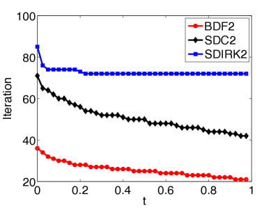
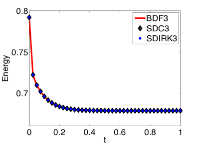
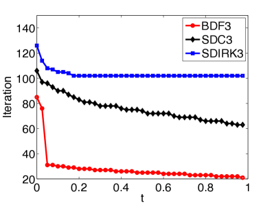
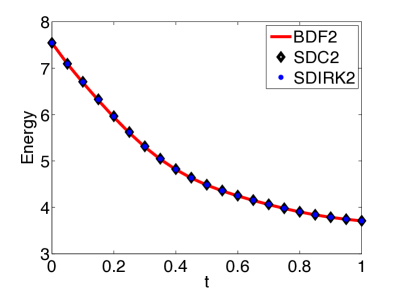
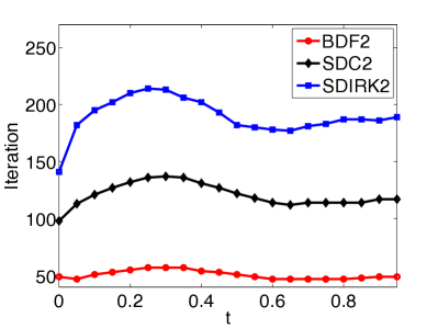
Figure 2. Energy descent and nonlinear iteration count history of all second- and third- order methods with fixed time step Δt=0.025Δ𝑡0.025\Delta t=0.025 and parameters (33).
Table 1. Refinement studies of second-order methods for 1D CH equation with periodic BC.
BDF2 SDIRK2 SDC2
ΔtΔ𝑡\Delta t Lsuperscript𝐿L^{\infty} error order Lsuperscript𝐿L^{\infty} error order Lsuperscript𝐿L^{\infty} error order
0.05000.05000.0500 0.000 029 4540.0000294540.000\,029\,454 - 0.000 004 778 70.00000477870.000\,004\,778\,7 - 0.000 063 7630.0000637630.000\,063\,763 -
0.02500.02500.0250 0.000 007 277 10.00000727710.000\,007\,277\,1 2.01702.01702.0170 0.000 001 205 00.00000120500.000\,001\,205\,0 1.98761.98761.9876 0.000 015 4120.0000154120.000\,015\,412 2.04872.04872.0487
0.01250.01250.0125 0.000 001 975 50.00000197550.000\,001\,975\,5 1.88121.88121.8812 0.000 000 300 810.000000300810.000\,000\,300\,81 2.00212.00212.0021 0.000 003 761 80.00000376180.000\,003\,761\,8 2.03452.03452.0345
0.00630.00630.0063 0.000 000 538 690.000000538690.000\,000\,538\,69 1.87471.87471.8747 0.000 000 075 0760.0000000750760.000\,000\,075\,076 2.00242.00242.0024 0.000 000 927 860.000000927860.000\,000\,927\,86 2.01942.01942.0194
0.00310.00310.0031 0.000 000 143 520.000000143520.000\,000\,143\,52 1.90821.90821.9082 0.000 000 018 7320.0000000187320.000\,000\,018\,732 2.00292.00292.0029 0.000 000 230 320.000000230320.000\,000\,230\,32 2.01032.01032.0103

.

The factorization of the Helmholtz operators is switched based on the time step size, and is different for each method:

BDF2: Δt=32ϵ2=0.0486,SDIRK2: Δt=ϵ21220.1106,SDC2: Δt=ϵ2=0.0324.formulae-sequenceBDF2: Δ𝑡32superscriptitalic-ϵ20.0486SDIRK2: Δ𝑡superscriptitalic-ϵ21220.1106SDC2: Δ𝑡superscriptitalic-ϵ20.0324\text{BDF2: }\Delta t=\frac{3}{2}\epsilon^{2}=0.0486,\quad\text{SDIRK2: }\Delta t=\frac{\epsilon^{2}}{1-\frac{\sqrt{2}}{2}}\approx 0.1106,\quad\text{SDC2: }\Delta t=\epsilon^{2}=0.0324.

Table 1 shows that all methods exhibit second order convergence. Moreover in Figure 2(a), we see that the total energy of each method decays during this time evolution.

In Figure 2(b), we plot the total iteration history of each scheme for the tolerance Ntol=1012subscript𝑁tolsuperscript1012N_{\text{tol}}=10^{-12}. The wall clock time (seconds) of BDF2, SDC2, SDIRK2 is 0.9725(s)0.9725𝑠0.9725(s), 1.9003(s)1.9003𝑠1.9003(s), and 2.6468(s)2.6468𝑠2.6468(s), respectively, for a final simulation time Tfinal=1subscript𝑇final1T_{\text{final}}=1; so the BDF2 method computationally the most efficient. We observe that SDIRK2 is the slowest, as a nonlinear solve is required for both stages K1subscript𝐾1K_{1} and K2subscript𝐾2K_{2}, at each time step.

Next, we compare the corresponding third-order schemes for the CH equation, with the same parameters in (33), and with the following considerations:

  • [BDF3] Need two initial steps: SDIRK2 used. (Switch criterion: Δtswitch=116ϵ2)Switch criterion: Δsubscript𝑡switch116superscriptitalic-ϵ2(\text{Switch criterion: }\Delta t_{\text{switch}}=\frac{11}{6}\epsilon^{2})

  • [SDIRK3] Need to compute K1,K2,K3subscript𝐾1subscript𝐾2subscript𝐾3K_{1},K_{2},K_{3} at each update. (Δtswitch=ϵ2η,η0.4359)formulae-sequenceΔsubscript𝑡switchsuperscriptitalic-ϵ2𝜂𝜂0.4359(\Delta t_{\text{switch}}=\frac{\epsilon^{2}}{\eta},\eta\approx 0.4359)

  • [SDC3] Compute from level [0] to level [2] with the quadrature order P𝑃P in (29): First, choose P=2𝑃2P=2 at level [2]delimited-[]2[2], then weights are q~0=512,q~1=812,q~2=112formulae-sequencesubscript~𝑞0512formulae-sequencesubscript~𝑞1812subscript~𝑞2112\tilde{q}_{0}=\dfrac{5}{12},\tilde{q}_{1}=\dfrac{8}{12},\tilde{q}_{2}=-\dfrac{1}{12}. (Δtswitch=ϵ2)Δsubscript𝑡switchsuperscriptitalic-ϵ2(\Delta t_{\text{switch}}=\epsilon^{2})

The energy and iteration history of third order schemes are shown in Figures 2(c) and 2(d). Again we see that the numerical energy decays. The beginning iteration number of BDF3 is larger than that of BDF2, since the initialization requires SDIRK2. But BDF3 is still the most efficient method of the third order schemes. The wall clock time (seconds) of BDF3, SDC3, SDIRK3 is 1.0355(s)1.0355𝑠1.0355(s), 2.8539(s)2.8539𝑠2.8539(s), and 3.6613(s)3.6613𝑠3.6613(s), respectively, for a final simulation time Tfinal=1subscript𝑇final1T_{\text{final}}=1.

The successive errors of third-order methods are shown in Table 2.

Table 2. Refinement studies of third-order methods for the 1D CH equation with periodic BC.
BDF3 SDIRK3 SDC3
ΔtΔ𝑡\Delta t Lsuperscript𝐿L^{\infty} error order Lsuperscript𝐿L^{\infty} error order Lsuperscript𝐿L^{\infty} error order
0.05000.05000.0500 0.000 016 0010.0000160010.000\,016\,001 - 0.000 001 725 90.00000172590.000\,001\,725\,9 - 0.000 012 6690.0000126690.000\,012\,669 -
0.02500.02500.0250 0.000 005 283 20.00000528320.000\,005\,283\,2 1.59871.59871.5987 0.000 000 361 180.000000361180.000\,000\,361\,18 2.25662.25662.2566 0.000 002 100 20.00000210020.000\,002\,100\,2 2.59272.59272.5927
0.01250.01250.0125 0.000 001 175 60.00000117560.000\,001\,175\,6 2.16802.16802.1680 0.000 000 062 8230.0000000628230.000\,000\,062\,823 2.52342.52342.5234 0.000 000 311 230.000000311230.000\,000\,311\,23 2.75452.75452.7545
0.00630.00630.0063 0.000 000 193 140.000000193140.000\,000\,193\,14 2.60572.60572.6057 0.000 000 009 616 30.00000000961630.000\,000\,009\,616\,3 2.70772.70772.7077 0.000 000 042 6150.0000000426150.000\,000\,042\,615 2.86862.86862.8686
0.00310.00310.0031 0.000 000 026 5060.0000000265060.000\,000\,026\,506 2.86522.86522.8652 0.000 000 001 301 10.00000000130110.000\,000\,001\,301\,1 2.88582.88582.8858 0.000 000 005 418 50.00000000541850.000\,000\,005\,418\,5 2.97542.97542.9754
0.00160.00160.0016 0.000 000 003 251 90.00000000325190.000\,000\,003\,251\,9 3.02703.02703.0270 0.000 000 000 174 470.000000000174470.000\,000\,000\,174\,47 2.89872.89872.8987 0.000 000 000 669 240.000000000669240.000\,000\,000\,669\,24 3.01733.01733.0173

Each method achieves third order convergence for small ΔtΔ𝑡\Delta t; but the order of convergence begins to plateau for larger time steps. To this end, SDC3 has a slight advantage. Indeed upon raising the polynomial order (29) from P=2𝑃2P=2 to P=3𝑃3P=3, which requires one more correction at each time step, we obtain third order accuracy even for large time steps, as shown in Table 3.

Table 3. Refinement study of SDC3 (P=3𝑃3P=3) for the 1D CH equation.
SDC3 (P=3𝑃3P=3)
ΔtΔ𝑡\Delta t Lsuperscript𝐿L^{\infty} error order
0.05000.05000.0500 0.000 009 946 20.00000994620.000\,009\,946\,2 -
0.02500.02500.0250 0.000 001 306 10.00000130610.000\,001\,306\,1 2.92892.92892.9289
0.01250.01250.0125 0.000 000 141 420.000000141420.000\,000\,141\,42 3.20723.20723.2072
0.00630.00630.0063 0.000 000 016 1550.0000000161550.000\,000\,016\,155 3.12993.12993.1299
0.00310.00310.0031 0.000 000 001 785 10.00000000178510.000\,000\,001\,785\,1 3.17793.17793.1779
0.00160.00160.0016 0.000 000 000 227 670.000000000227670.000\,000\,000\,227\,67 2.97102.97102.9710

5. Multiple spatial dimension

We now extend the 1D solver to multiple spatial dimensions via dimensional splitting [7, 5, 6]. We first write the 2D modified Helmholtz operator as

=IΔα2=(Ixxα2)(Iyyα2)xxyyα4xyxxyyα4,𝐼Δsuperscript𝛼2𝐼subscript𝑥𝑥superscript𝛼2𝐼subscript𝑦𝑦superscript𝛼2subscript𝑥𝑥subscript𝑦𝑦superscript𝛼4subscript𝑥subscript𝑦subscript𝑥𝑥subscript𝑦𝑦superscript𝛼4\mathcal{L}=I-\frac{\Delta}{\alpha^{2}}=\left(I-\frac{\partial_{xx}}{\alpha^{2}}\right)\left(I-\frac{\partial_{yy}}{\alpha^{2}}\right)-\frac{\partial_{xx}\partial_{yy}}{\alpha^{4}}\equiv\mathcal{L}_{x}\mathcal{L}_{y}-\frac{\partial_{xx}\partial_{yy}}{\alpha^{4}}, (34)

where xsubscript𝑥\mathcal{L}_{x} and ysubscript𝑦\mathcal{L}_{y} are univariate operators, and so the fourth order term represents a splitting error. Now x1superscriptsubscript𝑥1\mathcal{L}_{x}^{-1} is applied for fixed y𝑦y, and vice versa for y1superscriptsubscript𝑦1\mathcal{L}_{y}^{-1} in a line-by-line fashion, similar to alternating direction implicit (ADI) type method [12, 15]. Our key observation is that if we include the splitting error term from equation (34) in the fixed point iteration, then we can simultaneously solve the nonlinear problem, and correct the splitting error. More detailed analysis of the 2D CH equation (1) and 2D CH vector equations (4) will be presented below.

5.1. Semi-discrete solution to 2D CH equation

We now construct the semi-discrete scheme for the 2D CH equation, using the Backward Euler method. The analogous higher order schemes follow accordingly. Starting from the 1D scheme (17), we replace xxsubscript𝑥𝑥\partial_{xx} with the Laplacian operator Δ=xx+yyΔsubscript𝑥𝑥subscript𝑦𝑦\Delta=\partial_{xx}+\partial_{yy}. If Δt<ϵ2Δ𝑡superscriptitalic-ϵ2\Delta t<\epsilon^{2}, we complete the square of the operator, and have

(IΔα2)2[vn+1,k+1]=vn+ΔtΔ(fn+1,k2ϵ2Δtvn+1,k),superscript𝐼Δsuperscript𝛼22delimited-[]superscript𝑣𝑛1𝑘1superscript𝑣𝑛Δ𝑡Δsuperscript𝑓𝑛1𝑘2superscriptitalic-ϵ2Δ𝑡superscript𝑣𝑛1𝑘\left(I-\frac{\Delta}{\alpha^{2}}\right)^{2}[v^{n+1,k+1}]=v^{n}+\Delta t\Delta\left(f^{n+1,k}-2\sqrt{\frac{\epsilon^{2}}{\Delta t}}v^{n+1,k}\right), (35)

where 1α2=ϵ2Δt1superscript𝛼2superscriptitalic-ϵ2Δ𝑡\frac{1}{\alpha^{2}}=\sqrt{\epsilon^{2}\Delta t}. Plugging the identity in (34), by lagging the mixed derivative term along with the nonlinear term,

(xy)2[vn+1,k+1]=vn+ΔtΔ(fn+1,k2ϵ2Δtvn+1,k)+(2xxyyα4(xxyyα4)2)vn+1,ksuperscriptsubscript𝑥subscript𝑦2delimited-[]superscript𝑣𝑛1𝑘1superscript𝑣𝑛Δ𝑡Δsuperscript𝑓𝑛1𝑘2superscriptitalic-ϵ2Δ𝑡superscript𝑣𝑛1𝑘2subscript𝑥𝑥subscript𝑦𝑦superscript𝛼4superscriptsubscript𝑥𝑥subscript𝑦𝑦superscript𝛼42superscript𝑣𝑛1𝑘\left(\mathcal{L}_{x}\mathcal{L}_{y}\right)^{2}[v^{n+1,k+1}]=v^{n}+\Delta t\Delta\left(f^{n+1,k}-2\sqrt{\frac{\epsilon^{2}}{\Delta t}}v^{n+1,k}\right)+\left(2\frac{\partial_{xx}\partial_{yy}}{\alpha^{4}}-\left(\frac{\partial_{xx}\partial_{yy}}{\alpha^{4}}\right)^{2}\right)v^{n+1,k} (36)

Note that Laplacian operator and mixed derivative can be replaced as follows:

Δ=α2(Ixy+xxyyα4),xxyyα4=(xI)(yI).formulae-sequenceΔsuperscript𝛼2𝐼subscript𝑥subscript𝑦subscript𝑥𝑥subscript𝑦𝑦superscript𝛼4subscript𝑥𝑥subscript𝑦𝑦superscript𝛼4subscript𝑥𝐼subscript𝑦𝐼\Delta=\alpha^{2}\left(I-\mathcal{L}_{x}\mathcal{L}_{y}+\frac{\partial_{xx}\partial_{yy}}{\alpha^{4}}\right),\quad\frac{\partial_{xx}\partial_{yy}}{\alpha^{4}}=(\mathcal{L}_{x}-I)(\mathcal{L}_{y}-I).

Now we formally invert both operators to the right hand side of (36),

vn+1,k+1=(xy)2[vn]+(xy)1𝒞1[α2Δt(fn+1,k2ϵ2Δtvn+1,k)]+𝒞2[vn+1,k]superscript𝑣𝑛1𝑘1superscriptsubscript𝑥subscript𝑦2delimited-[]superscript𝑣𝑛superscriptsubscript𝑥subscript𝑦1subscript𝒞1delimited-[]superscript𝛼2Δ𝑡superscript𝑓𝑛1𝑘2superscriptitalic-ϵ2Δ𝑡superscript𝑣𝑛1𝑘subscript𝒞2delimited-[]superscript𝑣𝑛1𝑘v^{n+1,k+1}=\left(\mathcal{L}_{x}\mathcal{L}_{y}\right)^{-2}\left[v^{n}\right]+\left(\mathcal{L}_{x}\mathcal{L}_{y}\right)^{-1}\mathcal{C}_{1}[\alpha^{2}\Delta t(f^{n+1,k}-2\sqrt{\frac{\epsilon^{2}}{\Delta t}}v^{n+1,k})]+\mathcal{C}_{2}\left[v^{n+1,k}\right] (37)

where

𝒞1subscript𝒞1\displaystyle\mathcal{C}_{1} =(xy)1I+𝒟x𝒟y,𝒟γ=Iγ1,(γ={x,y})formulae-sequenceabsentsuperscriptsubscript𝑥subscript𝑦1𝐼subscript𝒟𝑥subscript𝒟𝑦subscript𝒟𝛾𝐼superscriptsubscript𝛾1𝛾𝑥𝑦\displaystyle=\left(\mathcal{L}_{x}\mathcal{L}_{y}\right)^{-1}-I+\mathcal{D}_{x}\mathcal{D}_{y},\quad\mathcal{D}_{\gamma}=I-\mathcal{L}_{\gamma}^{-1},(\gamma=\{x,y\}) (38)
𝒞2subscript𝒞2\displaystyle\mathcal{C}_{2} =2𝒟x𝒟y(𝒟x𝒟y)2.absent2subscript𝒟𝑥subscript𝒟𝑦superscriptsubscript𝒟𝑥subscript𝒟𝑦2\displaystyle=2\mathcal{D}_{x}\mathcal{D}_{y}-\left(\mathcal{D}_{x}\mathcal{D}_{y}\right)^{2}. (39)

As shown, every mixed-derivative splitting error term can be controlled by applying 𝒟γsubscript𝒟𝛾\mathcal{D}_{\gamma}, (γ={x,y}𝛾𝑥𝑦\gamma=\{x,y\}) operators, which can be constructed in a line-by-line fashion. We emphasize that this allows us to remove splitting error, which is O(1α4)=O(Δt)𝑂1superscript𝛼4𝑂Δ𝑡O(\frac{1}{\alpha^{4}})=O(\Delta t). Similar treatment of higher order BDF, SDIRK and SDC methods shows that the corresponding splitting errors can also be removed in this manner. Also, the fully discrete scheme follows from line-by-line spatial discretization, as outlined in Section 3.2.

We now consider the standard benchmark initial states in the 2D setting [9, 23], to confirm the temporal order of accuracy. The initial condition is

u0(x,y)=2e(sin(x)+sin(y)2)+2.2e(sin(x)sin(y)2)1,(x,y)[0,2π]2,formulae-sequencesubscript𝑢0𝑥𝑦2superscript𝑒𝑥𝑦22.2superscript𝑒𝑥𝑦21𝑥𝑦superscript02𝜋2u_{0}(x,y)=2e^{(\sin(x)+\sin(y)-2)}+2.2e^{(-\sin(x)-\sin(y)-2)}-1,\qquad(x,y)\in[0,2\pi]^{2}, (40)

with the periodic boundary conditions, and the following parameters

ϵ=0.18,Δx=2π1280.0491,Tfinal=1(0tTfinal),Ntol=106.formulae-sequenceformulae-sequenceitalic-ϵ0.18Δ𝑥2𝜋1280.0491formulae-sequencesubscript𝑇final10𝑡subscript𝑇finalsubscript𝑁tolsuperscript106\epsilon=0.18,\quad\Delta x=\dfrac{2\pi}{128}\approx 0.0491,\quad T_{\text{final}}=1\hskip 5.69054pt(0\leq t\leq T_{\text{final}}),\quad N_{\text{tol}}=10^{-6}. (41)

We use a 4thlimit-fromsuperscript4th4^{\text{th}}-order spatial quadrature to ensure that temporal error is dominant.

The temporal refinement study of each second-order scheme for the 2D CH equation is shown in Table 4. We observe the expected second-order of convergence for all three methods.

Table 4. Refinement studies of second-order methods for the 2D CH equation.
BDF2 SDIRK2 SDC2
ΔtΔ𝑡\Delta t Lsuperscript𝐿L^{\infty} error order Lsuperscript𝐿L^{\infty} error order Lsuperscript𝐿L^{\infty} error order
0.10000.10000.1000 0.003 789 10.00378910.003\,789\,1 - 0.001 025 00.00102500.001\,025\,0 - 0.002 333 40.00233340.002\,333\,4 -
0.05000.05000.0500 0.000 826 260.000826260.000\,826\,26 2.19722.19722.1972 0.000 269 500.000269500.000\,269\,50 1.92721.92721.9272 0.000 505 700.000505700.000\,505\,70 2.20612.20612.2061
0.02500.02500.0250 0.000 203 190.000203190.000\,203\,19 2.02382.02382.0238 0.000 069 7960.0000697960.000\,069\,796 1.94911.94911.9491 0.000 110 000.000110000.000\,110\,00 2.20072.20072.2007
0.01250.01250.0125 0.000 046 9090.0000469090.000\,046\,909 2.11492.11492.1149 0.000 017 8090.0000178090.000\,017\,809 1.97061.97061.9706 0.000 028 3120.0000283120.000\,028\,312 1.95811.95811.9581
Refer to caption
(a) Energy decay (2ndsuperscript2nd2^{\text{nd}} order methods)
Refer to caption
(b) Iteration count(2ndsuperscript2nd2^{\text{nd}} order methods)
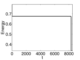
Figure 3. Energy descent and nonlinear iteration count history of all second-order 2D methods with fixed time step Δt=0.05Δ𝑡0.05\Delta t=0.05 and with parameters (41)

We also confirm the total energy, shown in Figure 3(a), is non-increasing during time evolution. Based on the iteration count, we see that BDF2 is the most efficient scheme, as was the case in 1D.

In principle, our method extends to even higher orders of accuracy in both time and space, as well as 3 spatial dimensions, since the splitting error technique in (38) can remove additional splitting errors.

5.2. Semi-discrete solution to 2D vector CH equation

We now extend our algorithm to vector CH (VCH) model (3). This model consists of two coupled variables u1subscript𝑢1u_{1} and u2subscript𝑢2u_{2} with local dynamic 𝐮Wsubscript𝐮𝑊\nabla_{\bf u}W, comprised of partial derivatives of 6thlimit-fromsuperscript6th6^{\text{th}}- order polynomials W(u1,u2)𝑊subscript𝑢1subscript𝑢2W(u_{1},u_{2}) defined in (4).

Before employing the MOLTT{}^{\text{T}} formulation to this system, we translate the vector (u1,u2)subscript𝑢1subscript𝑢2(u_{1},u_{2}) about its equilibrium state, which is based on the functional W(u1,u2)𝑊subscript𝑢1subscript𝑢2W(u_{1},u_{2}),

(u1,u2)={(cos(θi),sin(θi))|θ1=0,θ2=2π3,θ=2π3}{(1,0),(12,32),(12,32)}superscriptsubscript𝑢1superscriptsubscript𝑢2conditional-setsubscript𝜃𝑖subscript𝜃𝑖formulae-sequencesubscript𝜃10formulae-sequencesubscript𝜃22𝜋3𝜃2𝜋31012321232(u_{1}^{\ast},u_{2}^{\ast})=\left\{\left(\cos(\theta_{i}),\sin(\theta_{i})\right)\,\middle|\,\theta_{1}=0,\theta_{2}=\frac{2\pi}{3},\theta=-\frac{2\pi}{3}\right\}\equiv\left\{(1,0),(-\frac{1}{2},\frac{\sqrt{3}}{2}),(-\frac{1}{2},-\frac{\sqrt{3}}{2})\right\}

which are cube roots of unity in (u1,u2)subscript𝑢1subscript𝑢2(u_{1},u_{2}) plane. A straightforward calculation yields the Jacobian of the potential 𝐮Wsubscript𝐮𝑊\nabla_{\bf u}W evaluated at these points

𝒥𝐮W(u1,u2)[2Wu122Wu1u22Wu2u12Wu22](u1,u2)=[180018],subscript𝒥subscript𝐮𝑊superscriptsubscript𝑢1superscriptsubscript𝑢2subscriptmatrixsuperscript2𝑊superscriptsubscript𝑢12superscript2𝑊subscript𝑢1subscript𝑢2superscript2𝑊subscript𝑢2subscript𝑢1superscript2𝑊superscriptsubscript𝑢22superscriptsubscript𝑢1superscriptsubscript𝑢2matrix180018\mathcal{J}_{\nabla_{\bf u}W}(u_{1}^{\ast},u_{2}^{\ast})\equiv\begin{bmatrix}\frac{\partial^{2}W}{\partial u_{1}^{2}}&\frac{\partial^{2}W}{\partial u_{1}u_{2}}\\[3.00003pt] \frac{\partial^{2}W}{\partial u_{2}u_{1}}&\frac{\partial^{2}W}{\partial u_{2}^{2}}\end{bmatrix}_{(u_{1}^{\ast},u_{2}^{\ast})}=\begin{bmatrix}18&0\\[3.00003pt] 0&18\end{bmatrix}, (42)

hence all points are stable equilibrium solutions [23]. We subtract 𝐮=(u1,u2)𝐮subscript𝑢1subscript𝑢2{\bf{u}}=(u_{1},u_{2}) of the background state 𝐳3(12,32)subscript𝐳31232{\bf{z}}_{3}\equiv(-\frac{1}{2},-\frac{\sqrt{3}}{2}), and introduce the new transformed vector 𝐯=(v1,v2)=𝐮𝐳𝟑𝐯subscript𝑣1subscript𝑣2𝐮subscript𝐳3{\bf{v}}=(v_{1},v_{2})=\bf{u}-\bf{z}_{3} into the original system (3),

𝐯t=ϵ2Δ2𝐯+Δ𝐯W(𝐯+𝐳𝟑)ϵ2Δ2𝐯+Δ(𝐯W~(𝐯)+18𝐯)subscript𝐯𝑡superscriptitalic-ϵ2superscriptΔ2𝐯Δsubscript𝐯𝑊𝐯subscript𝐳3superscriptitalic-ϵ2superscriptΔ2𝐯Δsubscript𝐯~𝑊𝐯18𝐯{\bf{v}}_{t}=-\epsilon^{2}\Delta^{2}{\bf{v}}+\Delta\nabla_{\bf v}W\left(\bf{v}+\bf{z}_{3}\right)\equiv-\epsilon^{2}\Delta^{2}{\bf{v}}+\Delta\left(\nabla_{\bf v}\tilde{W}({\bf{v}})+18{\bf{v}}\right) (43)

where W~v1(𝐯):=Wv1(𝐯+𝐳𝟑)18v1assignsubscript~𝑊subscript𝑣1𝐯subscript𝑊subscript𝑣1𝐯subscript𝐳318subscript𝑣1\tilde{W}_{v_{1}}({\bf{v}}):=W_{v_{1}}({\bf{v}}+{\bf{z}_{3}})-18v_{1} and W~v2(𝐯):=Wv2(𝐯+𝐳𝟑)18v2assignsubscript~𝑊subscript𝑣2𝐯subscript𝑊subscript𝑣2𝐯subscript𝐳318subscript𝑣2\tilde{W}_{v_{2}}({\bf{v}}):=W_{v_{2}}({\bf{v}}+{\bf{z}_{3}})-18v_{2}.

The backward Euler scheme applied to the transformed system (43) results in

(I18ΔtΔ+ϵ2ΔtΔ2)𝐯n+1,k+1=𝐯n+Δ𝐯W~n+1,k𝐼18Δ𝑡Δsuperscriptitalic-ϵ2Δ𝑡superscriptΔ2superscript𝐯𝑛1𝑘1superscript𝐯𝑛Δsubscript𝐯superscript~𝑊𝑛1𝑘\displaystyle\left(I-18\Delta t\Delta+\epsilon^{2}\Delta t\Delta^{2}\right){\bf v}^{n+1,k+1}={\bf v}^{n}+\Delta\nabla_{\bf v}\tilde{W}^{n+1,k} (44)

where k𝑘k denotes the iteration index. We again introduce two factorizations of the left-hand side operator:

Δtϵ281::Δ𝑡superscriptitalic-ϵ281absent\displaystyle\Delta t\geq\frac{\epsilon^{2}}{81}:\quad I18ΔtΔ+ϵ2ΔtΔ2=(IΔα12)(IΔα22),𝐼18Δ𝑡Δsuperscriptitalic-ϵ2Δ𝑡superscriptΔ2𝐼Δsuperscriptsubscript𝛼12𝐼Δsuperscriptsubscript𝛼22\displaystyle I-18\Delta t\Delta+\epsilon^{2}\Delta t\Delta^{2}=\left(I-\frac{\Delta}{\alpha_{1}^{2}}\right)\left(I-\frac{\Delta}{\alpha_{2}^{2}}\right), (45)
Δt<ϵ281::Δ𝑡superscriptitalic-ϵ281absent\displaystyle\Delta t<\frac{\epsilon^{2}}{81}:\quad I2ϵ2ΔtΔ+ϵ2ΔtΔ2=(IΔα2)2,𝐼2superscriptitalic-ϵ2Δ𝑡Δsuperscriptitalic-ϵ2Δ𝑡superscriptΔ2superscript𝐼Δsuperscript𝛼22\displaystyle I-2\sqrt{\epsilon^{2}\Delta t}\Delta+\epsilon^{2}\Delta t\Delta^{2}=\left(I-\frac{\Delta}{\alpha^{2}}\right)^{2}, (46)

where

1αi2=9Δt±81Δt2ϵ2Δt,1α2=ϵ2Δt.formulae-sequence1superscriptsubscript𝛼𝑖2plus-or-minus9Δ𝑡81Δsuperscript𝑡2superscriptitalic-ϵ2Δ𝑡1superscript𝛼2superscriptitalic-ϵ2Δ𝑡\frac{1}{\alpha_{i}^{2}}=9\Delta t\pm\sqrt{81\Delta t^{2}-\epsilon^{2}\Delta t},\qquad\frac{1}{\alpha^{2}}=\sqrt{\epsilon^{2}\Delta t}.

Inversion of the above operators follows from the same strategy as in Section 5.1. As expected, the stabilized fixed point iteration (45) permits larger time steps without limiting the foregoing energy stability property (5).

6. Adaptive time stepping

For phase-field models, adaptive time stepping is a crucial feature for an efficient and accurate numerical solution. For instance, the solution of CH equation (1) evolves on various time scales. During spinodal evolution, transition layers are developed in O(1)𝑂1O(1) time. Subsequently, they slowly evolve and merge on a longer time scale, O(eC/ϵ)𝑂superscript𝑒𝐶italic-ϵO(e^{C/\epsilon}) for 1D, which is called ripening process. Simulating these phenomena with a fixed time stepping necessarily becomes inefficient, and so we must incorporate adaptive time into our above MOLTT{}^{\text{T}} schemes.

The adaptive time step size control is based on the Local Truncation Error(LTE) ηesubscript𝜂𝑒\eta_{e} at each time level t=tn𝑡superscript𝑡𝑛t=t^{n}. The LTE can be approximated by ηeη=uunsubscript𝜂𝑒𝜂subscriptnormsuperscript𝑢superscript𝑢𝑛\eta_{e}\approx\eta=||u^{\ast}-u^{n}||_{\infty}, where usuperscript𝑢u^{\ast} is an explicit predictor solution, typically using the Forward Euler (FE) or Adams Bashforth (AB) schemes [9]. On the other hand, Richardson extrapolation (known as step-doubling) or embedded Runge-Kutta pairs can also be used [10]. Below we will compare LTE estimates based on Richardson extrapolation, as well BDF2 and SDC2 predictors. The time step size selection criteria presented in [9] will be used, which is summarized in algorithm 1 below.

Algorithm 1 Adaptive time step-size control
  1. (1)

    Starting at t=tn𝑡superscript𝑡𝑛t=t^{n}, approximate the local truncation error. For Richardson extrapolation, the solution is estimated twice: once with a full step ΔtΔ𝑡\Delta t (denoted by uΔtn+1subscriptsuperscript𝑢𝑛1Δ𝑡u^{n+1}_{\Delta t}), and again with two half steps (uΔt/2n+1subscriptsuperscript𝑢𝑛1Δ𝑡2u^{n+1}_{\Delta t/2}). The difference between the two numerical approximations gives an estimate for the LTE of un+1superscript𝑢𝑛1u^{n+1}

    (Richardson extrapolation)ηeη:=12uΔtn+1uΔt/2n+1.(Richardson extrapolation)subscript𝜂𝑒𝜂assign12subscriptnormsubscriptsuperscript𝑢𝑛1Δ𝑡subscriptsuperscript𝑢𝑛1Δ𝑡2\text{(Richardson extrapolation)}\quad\eta_{e}\approx\eta:=\frac{1}{2}||u^{n+1}_{\Delta t}-u^{n+1}_{\Delta t/2}||_{\infty}.
  2. (2)

    Define a tolerance σtolsubscript𝜎tol\sigma_{\text{tol}} for the above LTE. If the accuracy criterion is not met (η>σtol𝜂subscript𝜎tol\eta>\sigma_{\text{tol}}), then the time step is reduced. If the desired accuracy is achieved, then we test for the following criteria,

    1. (I)

      ησtol::𝜂subscript𝜎tolabsent\eta\leq\sigma_{\text{tol}}:

      NitNmaxit<0.7::subscript𝑁itsubscript𝑁it0.7absent\displaystyle\frac{N_{\text{it}}}{N_{\max\text{it}}}<0.7: Δtn+1=Δtnmin(θσtolη,γ),θ=0.8,γ=1.3>1formulae-sequenceΔsuperscript𝑡𝑛1Δsuperscript𝑡𝑛𝜃subscript𝜎tol𝜂𝛾formulae-sequence𝜃0.8𝛾1.31\displaystyle\quad\Delta t^{n+1}=\Delta t^{n}\cdot\min\left(\theta\sqrt{\frac{\sigma_{\text{tol}}}{\eta}},\gamma\right),\quad\theta=0.8,\quad\gamma=1.3>1
      0.7NitNmaxit<1::0.7subscript𝑁itsubscript𝑁it1absent\displaystyle 0.7\leq\frac{N_{\text{it}}}{N_{\max\text{it}}}<1: Δtn+1=Δtnmin(θσtolη,1),Δsuperscript𝑡𝑛1Δsuperscript𝑡𝑛𝜃subscript𝜎tol𝜂1\displaystyle\quad\Delta t^{n+1}=\Delta t^{n}\cdot\min\left(\theta\sqrt{\frac{\sigma_{\text{tol}}}{\eta}},1\right),
      NitNmaxit1::subscript𝑁itsubscript𝑁it1absent\displaystyle\frac{N_{\text{it}}}{N_{\max\text{it}}}\geq 1: Step fails.Reduce time step Δtn=Δtn1γStep fails.Reduce time step Δsuperscript𝑡𝑛Δsuperscript𝑡𝑛1𝛾\displaystyle\quad\text{Step fails.}\quad\text{Reduce time step }\Delta t^{n}=\Delta t^{n}\cdot\frac{1}{\gamma}
    2. (II)

      η>σtol:Step fails.Reduce time step\eta>\sigma_{\text{tol}}:\quad\text{Step fails.}\quad\text{Reduce time step}

      ησtol>2::𝜂subscript𝜎tol2absent\displaystyle\frac{\eta}{\sigma_{\text{tol}}}>2: Δtn=Δtn1γ,Δsuperscript𝑡𝑛Δsuperscript𝑡𝑛1𝛾\displaystyle\quad\Delta t^{n}=\Delta t^{n}\cdot\frac{1}{\gamma},
      ησtol2::𝜂subscript𝜎tol2absent\displaystyle\frac{\eta}{\sigma_{\text{tol}}}\leq 2: Δtn=ΔtnθσtolηΔsuperscript𝑡𝑛Δsuperscript𝑡𝑛𝜃subscript𝜎tol𝜂\displaystyle\quad\Delta t^{n}=\Delta t^{n}\cdot\theta\sqrt{\frac{\sigma_{\text{tol}}}{\eta}}

      where γ𝛾\gamma and θ𝜃\theta are the same safety factors defined in [9].

In practice, this procedure leads to small time steps during spinodal evolution, or at the ripening event, to maintain a consistent LTE. On the other hand, during slow coarsening (metastable states), small time steps are unnecessary and so ΔtΔ𝑡\Delta t is increased within the upper bound for fixed-point iteration count.

7. Numerical Results

In this section we present adaptive time stepping results using the previously developed MOLTT{}^{\text{T}} schemes.

7.1. 1D CH model

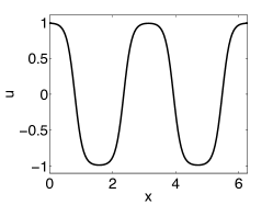
We first solve the 1D CH equation (1) with a stiff initial condition (32) (ϵ=0.18)italic-ϵ0.18(\epsilon=0.18). The second perturbation term of this initial state creates two intervals, u=1𝑢1u=-1 and u=+1𝑢1u=+1, which are asymmetric, so that a finite number of transition layers are formed during spinodal evolution. After a long ripening process, such layers are eventually absorbed into one region, at the so-called ripening time [9]. The aim of this simulation is to accurately capture all time scales using both fixed and adaptive time stepping strategies. (The spatial mesh size is fixed at Δx=2π1280.05Δ𝑥2𝜋1280.05\Delta x=\frac{2\pi}{128}\approx 0.05.)

In the first experiment, we implement our various time stepping schemes, with small fixed time step (Δt=0.01Δ𝑡0.01\Delta t=0.01). The ripening time Trsubscript𝑇rT_{\text{r}} is defined as that for which the midpoint value u(π,t)𝑢𝜋𝑡u(\pi,t) changes from positive to negative. The fixed point iteration has residual tolerance 1011superscript101110^{-11} at each step, and the ripening times are presented in Table 5. Our results agree well with the reference time Tr=8318.63subscript𝑇r8318.63T_{\text{r}}=8318.63 in [9].

Table 5. Ripening time of 1D CH equation with small fixed time (Δt=0.01)Δ𝑡0.01(\Delta t=0.01)
       Ripening time
BE        8317.818317.818317.81
BDF2        8318.708318.708318.70
BDF3        8318.748318.748318.74
SDC2        8318.998318.998318.99
SDC3        8318.848318.848318.84

We also compare the ripening time using several schemes, with larger fixed time steps in Table 6.

Table 6. Ripening time of 1D CH equation with larger fixed time step sizes.
    time step        Ripening time        Times(s)𝑠(s)
101010        8250.008250.008250.00        313.38313.38313.38
BE 111        8296.008296.008296.00        351.52351.52351.52
0.050.050.05        8311.858311.858311.85        1312.161312.161312.16
101010        9050.009050.009050.00        717.26717.26717.26
SDC2 111        8582.008582.008582.00        692.65692.65692.65
0.050.050.05        8319.808319.808319.80        2779.612779.612779.61
101010        8290.008290.008290.00        231.40231.40231.40
BDF2 111        8303.008303.008303.00        281.56281.56281.56
0.050.050.05        8315.758315.758315.75        1288.681288.681288.68

Among the three methods, BDF2 is the most efficient, and provides better estimates of the true ripening time, even for larger ΔtΔ𝑡\Delta t. In the most extreme instance of Δt=10Δ𝑡10\Delta t=10, we note that the first-order scheme (BE) predicts ripening too soon, and that SDC2 is too late; but BDF2 is still fairly accurate. However, to capture the ripening moment accurately, we still require small fixed time steps (Δt0.05Δ𝑡0.05\Delta t\leq 0.05), which is too expensive for long time simulations.

Table 7. Ripening time of 1D CH equation with adaptive time stpe size.
    δtolsubscript𝛿tol\delta_{\text{tol}}        Ripening time        Times(s)𝑠(s)
103superscript10310^{-3}        8292.548292.548292.54        224.03224.03224.03
BE 104superscript10410^{-4}        8276.088276.088276.08        226.06226.06226.06
(Richardson) 105superscript10510^{-5}        8308.238308.238308.23        235.44235.44235.44
103superscript10310^{-3}        8311.088311.088311.08        233.38233.38233.38
BE-SDC2 104superscript10410^{-4}        8311.478311.478311.47        239.58239.58239.58
105superscript10510^{-5}        8312.918312.918312.91        226.43226.43226.43
103superscript10310^{-3}        8320.038320.038320.03        184.71184.71184.71
BE-BDF2 104superscript10410^{-4}        8319.918319.918319.91        196.82196.82196.82
105superscript10510^{-5}        8317.878317.878317.87        208.18208.18208.18

Thus, we consider adaptive time stepping for the same problem. As indicated in Section 6, the local truncation error (LTE) can be approximated with Richardson extrapolation, or a higher order solver such as BDF2 or SDC2.

We implement three methods with the same fixed point residual tolerance 1011superscript101110^{-11}, Nmaxit=600subscript𝑁it600N_{\max\text{it}}=600 in Algorithm 1, but with various error tolerance δtolsubscript𝛿tol\delta_{\text{tol}}. The performance of the time-adaptive scheme is shown in Table 7. We see that time adaptivity is superior to fixed time stepping both in terms of accuracy and time to solution. Additionally, the BDF2 method is the most efficient predictor.
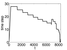
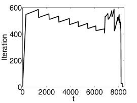
Refer to caption
(a) Time step size
Refer to caption
(b) Iteration count
Refer to caption
(c) Energy
Figure 4. Adaptive time stepping with the BE-BDF2 strategy.
Refer to caption
(a) u(x,0)𝑢𝑥0u(x,0)
Refer to caption
(b) u(x,0.51)𝑢𝑥0.51u(x,0.51)
Refer to caption
(c) u(x,3669.8)𝑢𝑥3669.8u(x,3669.8)
Refer to caption
(d) u(x,7005.7)𝑢𝑥7005.7u(x,7005.7)
Refer to caption
(e) u(x,8317.9)𝑢𝑥8317.9u(x,8317.9)
Refer to caption
(f) u(x,8319.2)𝑢𝑥8319.2u(x,8319.2)
Figure 5. Spinodal evolution for the 1D CH equation using adaptive time stepping (BE-BDF2).

In Figure 4 we plot the time step size, fixed-point iteration history and energy of numerical solutions obtained by the BE-BDF2 strategy (δtol=105subscript𝛿tolsuperscript105\delta_{\text{tol}}=10^{-5}). As shown in Figure 4(a), small time steps are used at early stage (spinodal evolution) but increase when the coarsening process starts, which speeds up the simulation without a loss of accuracy. If the iteration count is too large (NitNmaxitsubscript𝑁itsubscript𝑁itN_{\text{it}}\geq N_{\max\text{it}}), we reject the solution and compute u(x,t)𝑢𝑥𝑡u(x,t) again with reduced ΔtΔ𝑡\Delta t. We see this behavior in Figure 4(b), where time steps are decreased whenever NitNmaxitsubscript𝑁itsubscript𝑁itN_{\text{it}}\approx N_{\max\text{it}}. We also observe in Figure 4(c) that adaptive time stepping does not affect energy decay.

The phase function u(x,t)𝑢𝑥𝑡u(x,t) obtained by our numerical scheme is shown in Figure 5. The initial state 5(a) quickly moves to the metastable state 5(b), and then finally reaches the stable state 5(f) at which two layers are merged together after a long time. This simulation also shows that the ripening event happens over a very fast time scale in Figure 5(e).

7.2. 2D CH model

We next solve the CH equation (1) in two spatial dimensions. The parameters are

ϵ=0.18,Δx=Δy=2π1280.0491,Nmaxit=300,Ntol=106,formulae-sequenceformulae-sequenceitalic-ϵ0.18Δ𝑥Δ𝑦2𝜋1280.0491formulae-sequencesubscript𝑁it300subscript𝑁tolsuperscript106\epsilon=0.18,\quad\Delta x=\Delta y=\frac{2\pi}{128}\approx 0.0491,\quad N_{\max\text{it}}=300,\quad N_{\text{tol}}=10^{-6},

and the initial condition is (40). We first use BE, BDF2, and BDF3 with a small time step (Δt=0.05Δ𝑡0.05\Delta t=0.05) and check the ripening time, which is defined such that u(π2,π2)𝑢𝜋2𝜋2u(\frac{\pi}{2},\frac{\pi}{2}) changes from positive to negative. Based on the results summarized in Figure 6, we can define such ripening time as Tr=80.10subscript𝑇r80.10T_{\text{r}}=80.10. In addition, we note that raising the order of the scheme reduces the number of iterations per time step, and so the overall computational time is lower.
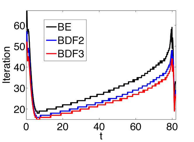
Refer to caption
       Ripening time        Run Time (s)𝑠(s)
BE        79.9579.9579.95        630.16630.16630.16
BDF2        80.1080.1080.10        526.19526.19526.19
BDF3        80.1080.1080.10        481.86481.86481.86
Figure 6. Ripening time of 2D CH equation with small fixed time (Δt=0.01)Δ𝑡0.01(\Delta t=0.01)
Refer to caption
(a) Time step size
Refer to caption
(b) Iteration count
Refer to caption
(c) Energy
Figure 7. Adaptive time stepping for 2D, with the BE-BDF2 strategy.

Next, we simulate the same problem with adaptive time step method (BE-BDF2). The time step history, number of nonlinear iterations, and energy history are presented in Figure 7. The 2D results are comparable to those from 1D in Section 7.1, in that larger time step sizes are used during coarsening, and smaller steps are required only to capture ripening (see Figure 7(a)). The energy in Figure 7(c) indicates that there are two sharp transitions in the energy \mathcal{E}; early on, and at ripening. Finally, we also observe the desired energy decay.
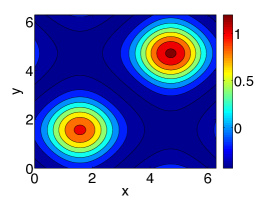
Refer to caption
(a) u(x,y,0)𝑢𝑥𝑦0u(x,y,0)
Refer to caption
(b) u(x,y,0.5083)𝑢𝑥𝑦0.5083u(x,y,0.5083)
Refer to caption
(c) u(x,y,15.807)𝑢𝑥𝑦15.807u(x,y,15.807)
Refer to caption
(d) u(x,y,70.015)𝑢𝑥𝑦70.015u(x,y,70.015)
Refer to caption
(e) u(x,y,80.536)𝑢𝑥𝑦80.536u(x,y,80.536)
Refer to caption
(f) u(x,y,90)𝑢𝑥𝑦90u(x,y,90)
Figure 8. Temporal evolution of the 2D CH solution with initial condition (40).

The contour plots of time evolution of the phase function u(x,y,t)𝑢𝑥𝑦𝑡u(x,y,t) are shown in Figure 8. The initial states 8(a) quickly reaches the metastable state, where we see two circular formations. Eventually the larger one absorbs the smaller, although over a very long time scale, shown in 8(c) - 8(e). The final state is shown in 8(f), where the larger region has fully consumed the smaller. In all plots, the total volume is preserved.

7.3. 2D CH vector model

We next apply our scheme from Section 5.2 to the 2D CH system (3), with our adaptive time stepping strategy. We use the same initial condition (40) for u1subscript𝑢1u_{1} and

u2(x,y,0)=sin(y),(x,y)[0,2π]2formulae-sequencesubscript𝑢2𝑥𝑦0𝑦𝑥𝑦superscript02𝜋2u_{2}(x,y,0)=\sin(y),\qquad(x,y)\in[0,2\pi]^{2} (47)

for u2subscript𝑢2u_{2} in the reference [9], and observe the long time behavior of the phase function 𝐮=(u1,u2)𝐮subscript𝑢1subscript𝑢2{\bf u}=(u_{1},u_{2}). With the parameters

ϵ=0.32,Δx=Δy=2π640.0982,Nmaxit=400,Ntol=106,δtol=1e4formulae-sequenceformulae-sequenceitalic-ϵ0.32Δ𝑥Δ𝑦2𝜋640.0982formulae-sequencesubscript𝑁it400formulae-sequencesubscript𝑁tolsuperscript106subscript𝛿tol1𝑒4\epsilon=0.32,\Delta x=\Delta y=\frac{2\pi}{64}\approx 0.0982,\quad N_{\max\text{it}}=400,\quad N_{\text{tol}}=10^{-6},\quad\delta_{\text{tol}}=1e-4

we implement BE-BDF2 adaptive scheme for VCH model.
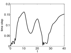
Refer to caption
(a) Time step size
Refer to caption
(b) Iteration count
Refer to caption
(c) Energy
Figure 9. The time step, iteration count, and energy history of VCH solution.

The contour plots of cos(arg(u1+iu2))subscript𝑢1𝑖subscript𝑢2\cos(\arg(u_{1}+iu_{2})) are shown in Figure 10. Instead of plotting u1subscript𝑢1u_{1} and u2subscript𝑢2u_{2} separately, [9] we define the angle θarg(u1+iu2)𝜃subscript𝑢1𝑖subscript𝑢2\theta\equiv\arg(u_{1}+iu_{2}) at a triple junction, and plot cos(θ)𝜃\cos(\theta) to avoid any discontinuities. We follow this benchmark plot using our numerical solution.
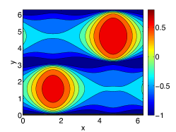
Refer to caption
(a) t=0𝑡0t=0
Refer to caption
(b) t=0.02503𝑡0.02503t=0.02503
Refer to caption
(c) t=0.5083𝑡0.5083t=0.5083
Refer to caption
(d) t=5.0848𝑡5.0848t=5.0848
Refer to caption
(e) t=20.128𝑡20.128t=20.128
Refer to caption
(f) t=24.286𝑡24.286t=24.286
Refer to caption
(g) t=25.005𝑡25.005t=25.005
Refer to caption
(h) t=30.021𝑡30.021t=30.021
Refer to caption
(i) t=40.015𝑡40.015t=40.015
Figure 10. Temporal evolution of the 2D CH vector solution with the initial (40) for u1subscript𝑢1u_{1} and (47) for u2subscript𝑢2u_{2}. Contours of cos(argu1+iu2)subscript𝑢1𝑖subscript𝑢2\cos(\arg u_{1}+iu_{2}) are plotted.

After some initial ripening in Figure 10(b), the interfaces dividing the three states 𝐮=𝐳𝐢𝐮subscript𝐳𝐢\bf{u}=\bf{z}_{i} (i=1,2,3)𝑖123(i=1,2,3) form around T=0.5𝑇0.5T=0.5. In Figure 10(c) - 10(i), two of the values have cos(2π/3)𝑐𝑜𝑠2𝜋3cos(2\pi/3) (light blue in the plots) but separated by dark blue lines. Then the ripening process begins, and occurs over a long time scale, ending around T=24.286𝑇24.286T=24.286 in Figure 10(f). Again, we remark that the volume is preserved over all time steps. For a more involved discussion of this simulation, we refer the interested reader to [9]. Our goal here is to demonstrate that our MOLTT{}^{\text{T}} scheme captures the correct ripening behavior.

7.4. 2D 6thsuperscript6th6^{\text{th}} order model

We also consider the 6thsuperscript6th6^{\text{th}} order problem:

ut=Δ[(ϵ2Δf(u)+ϵ2η)(ϵ2Δuf(u))],f(u)=u3u.formulae-sequencesubscript𝑢𝑡Δdelimited-[]superscriptitalic-ϵ2Δsuperscript𝑓𝑢superscriptitalic-ϵ2𝜂superscriptitalic-ϵ2Δ𝑢𝑓𝑢𝑓𝑢superscript𝑢3𝑢u_{t}=\Delta\left[(\epsilon^{2}\Delta-f^{\prime}(u)+\epsilon^{2}\eta)(\epsilon^{2}\Delta u-f(u))\right],\quad f(u)=u^{3}-u. (48)

where ϵitalic-ϵ\epsilon and η𝜂\eta are given positive constants. This problem is motivated by the functionalized Cahn-Hilliard (FCH) equation [18] which models interfacial energy in amphiphilic phase-separated mixtures. We follow a similar approach as before, and introduce the transformed variable v=u+1𝑣𝑢1v=u+1. Substitution into (48) results in

vt=Δ[(ϵ2Δf(v)+ϵ2η)(ϵ2Δvf(v))],f(v)=v33v2+2v.formulae-sequencesubscript𝑣𝑡Δdelimited-[]superscriptitalic-ϵ2Δsuperscript𝑓𝑣superscriptitalic-ϵ2𝜂superscriptitalic-ϵ2Δ𝑣𝑓𝑣𝑓𝑣superscript𝑣33superscript𝑣22𝑣v_{t}=\Delta\left[(\epsilon^{2}\Delta-f^{\prime}(v)+\epsilon^{2}\eta)(\epsilon^{2}\Delta v-f(v))\right],\quad f(v)=v^{3}-3v^{2}+2v. (49)

We again apply the backward Euler (BE) scheme for time discretization of (49), so that

(IΔtϵ4Δ3)vn+1=vnΔtΔ(ϵ2Δfn+1ϵ2(fΔv)n+1+(ff)n+1+ηϵ4Δvn+1ηϵ2fn+1)𝐼Δ𝑡superscriptitalic-ϵ4superscriptΔ3superscript𝑣𝑛1superscript𝑣𝑛Δ𝑡Δsuperscriptitalic-ϵ2Δsuperscript𝑓𝑛1superscriptitalic-ϵ2superscriptsuperscript𝑓Δ𝑣𝑛1superscript𝑓superscript𝑓𝑛1𝜂superscriptitalic-ϵ4Δsuperscript𝑣𝑛1𝜂superscriptitalic-ϵ2superscript𝑓𝑛1\displaystyle\left(I-\Delta t\epsilon^{4}\Delta^{3}\right)v^{n+1}=v^{n}-\Delta t\Delta\left(\epsilon^{2}\Delta f^{n+1}-\epsilon^{2}(f^{\prime}\Delta v)^{n+1}+(ff^{\prime})^{n+1}+\eta\epsilon^{4}\Delta{v}^{n+1}-\eta\epsilon^{2}{f}^{n+1}\right)

Hence, we invert the 6thsuperscript6th6^{\text{th}} order operator to solve vn+1superscript𝑣𝑛1v^{n+1}. One can invert this by completing the cube such that

(IΔtϵ43Δ)3vn+1=vnsuperscript𝐼3Δ𝑡superscriptitalic-ϵ4Δ3superscript𝑣𝑛1limit-fromsuperscript𝑣𝑛\displaystyle\left(I-\sqrt[3]{\Delta t\epsilon^{4}}\Delta\right)^{3}v^{n+1}=v^{n}- ΔtΔ(ϵ2Δfn+1ϵ2(fΔv)n+1+(ff)n+1+ηϵ4Δvn+1ηϵ2fn+1)Δ𝑡Δsuperscriptitalic-ϵ2Δsuperscript𝑓𝑛1superscriptitalic-ϵ2superscriptsuperscript𝑓Δ𝑣𝑛1superscript𝑓superscript𝑓𝑛1𝜂superscriptitalic-ϵ4Δsuperscript𝑣𝑛1𝜂superscriptitalic-ϵ2superscript𝑓𝑛1\displaystyle\Delta t\Delta\left(\epsilon^{2}\Delta f^{n+1}-\epsilon^{2}(f^{\prime}\Delta v)^{n+1}+(ff^{\prime})^{n+1}+\eta\epsilon^{4}\Delta{v}^{n+1}-\eta\epsilon^{2}{f}^{n+1}\right)
(3Δtϵ43Δ3(Δtϵ43)2Δ2)vn+1.33Δ𝑡superscriptitalic-ϵ4Δ3superscript3Δ𝑡superscriptitalic-ϵ42superscriptΔ2superscript𝑣𝑛1\displaystyle-\left(3\sqrt[3]{\Delta t\epsilon^{4}}\Delta-3(\sqrt[3]{\Delta t\epsilon^{4}})^{2}\Delta^{2}\right)v^{n+1}. (50)

We can now solve vn+1superscript𝑣𝑛1v^{n+1} by applying the triple inversion of our modified Helmholtz operator =IΔtϵ43Δ𝐼3Δ𝑡superscriptitalic-ϵ4Δ\mathcal{L}=I-\sqrt[3]{\Delta t\epsilon^{4}}\Delta by the same procedure in Section 5.1.
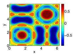
Refer to caption
(a) u(x,y,0)𝑢𝑥𝑦0u(x,y,0)
Refer to caption
(b) u(x,y,2)𝑢𝑥𝑦2u(x,y,2)
Refer to caption
(c) u(x,y,50)𝑢𝑥𝑦50u(x,y,50)
Refer to caption
(d) u(x,y,150)𝑢𝑥𝑦150u(x,y,150)
Refer to caption
(e) u(x,y,300)𝑢𝑥𝑦300u(x,y,300)
Refer to caption
(f) u(x,y,500)𝑢𝑥𝑦500u(x,y,500)
Figure 11. Temporal evolution of the 2D FCH equation with initial condition (40).

For simplicity, we apply the first-order BE scheme (50) with a fixed time step Δt=0.1Δ𝑡0.1\Delta t=0.1 to solve the 6thsuperscript6th6^{\text{th}} order problem (49) (η=1)𝜂1(\eta=1). By starting with the same initial condition (40) (ϵ=0.18)italic-ϵ0.18(\epsilon=0.18), and with the following parameters:

Δx=Δy=2π1280.05,Nmaxit=200,Ntol=106.formulae-sequenceΔ𝑥Δ𝑦2𝜋1280.05formulae-sequencesubscript𝑁it200subscript𝑁tolsuperscript106\Delta x=\Delta y=\frac{2\pi}{128}\approx 0.05,\quad N_{\max\text{it}}=200,\quad N_{\text{tol}}=10^{-6}.

The contour plots of our numerical solutions of (48) are shown in Figure 11. As expected [9], we can confirm that the final state becomes a regular array in Figure 11(f).

8. Conclusion

In this paper we have illustrated how the method of lines transpose (MOLT) can be used to solve nonlinear phase field models, particularly the Cahn Hilliard, vector Cahn-Hilliard, and functionalized Cahn-Hilliard equations. We utilize a novel factorization of the semi-discrete equation to ensure gradient stability, permitting large time steps. When combined with time adaptivity, we are able to resolve rapid events such as spinodal evolution, which occur after long meta stable states.

The spatial solver is matrix free, O(N)𝑂𝑁O(N), and logically Cartesian, and the splitting error is directly incorporated into the nonlinear fixed point iterations. We have considered higher order time stepping, such as backward difference formulas, implicit Runge-Kutta, and spectral deferred correction methods. Of all possible configurations, the time adaptive backward Euler-backward difference 2 (BE-BDF2) method is the most efficient in terms of accuracy and time to solution.

References

  • [1] R. Alexander. Diagonally implicit runge-kutta methods for stiff ode’s. SIAM Journal on Numerical Analysis, 14(6):1006–1021, 1977.
  • [2] L. Bronsard and F. Reitich. On three-phase boundary motion and the singular limit of a vector-valued ginzburg-landau equation. Archive for Rational Mechanics and Analysis, 124(4):355–379, 1993.
  • [3] J. W. Cahn and J. E. Hilliard. Free energy of a nonuniform system. i. interfacial free energy. The Journal of chemical physics, 28(2):258–267, 1958.
  • [4] M. Causley, A. Christlieb, B. Ong, and L. Van Groningen. Method of lines transpose: An implicit solution to the wave equation. Mathematics of Computation, 83(290):2763–2786, 2014.
  • [5] M. Causley, A. Christlieb, and E. Wolf. Method of lines transpose: an efficient a-stable solver for wave propagation. Journal of Scientific Computing, pages 1–26, 2016.
  • [6] M. F. Causley, H. Cho, A. J. Christlieb, and D. C. Seal. Method of lines transpose: High order l-stable o(n)𝑜𝑛o(n) schemes for parabolic equations using successive convolution. SIAM Journal on Numerical Analysis, 54(3):1635–1652, 2016.
  • [7] M. F. Causley and A. J. Christlieb. Higher order a-stable schemes for the wave equation using a successive convolution approach. SIAM Journal on Numerical Analysis, 52(1):220–235, 2014.
  • [8] L.-Q. Chen. Phase-field models for microstructure evolution. Annual review of materials research, 32(1):113–140, 2002.
  • [9] A. Christlieb, J. Jones, K. Promislow, B. Wetton, and M. Willoughby. High accuracy solutions to energy gradient flows from material science models. Journal of Computational Physics, 257:193–215, 2014.
  • [10] A. Christlieb, C. Macdonald, B. Ong, and R. Spiteri. Revisionist integral deferred correction with adaptive step-size control. Communications in Applied Mathematics and Computational Science, 10(1):1–25, 2015.
  • [11] A. Christlieb, K. Promislow, and Z. Xu. On the unconditionally gradient stable scheme for the cahn-hilliard equation and its implementation with fourier method. Commun. Math. Sci, 11:345–360, 2013.
  • [12] J. Douglas, Jr. On the numerical integration of 2ux2+2uy2=utsuperscript2𝑢superscript𝑥2superscript2𝑢superscript𝑦2𝑢𝑡\frac{\partial^{2}u}{\partial x^{2}}+\frac{\partial^{2}u}{\partial y^{2}}=\frac{\partial u}{\partial t} by implicit methods. Journal of the society for industrial and applied mathematics, 3(1):42–65, 1955.
  • [13] A. Dutt, L. Greengard, and V. Rokhlin. Spectral deferred correction methods for ordinary differential equations. BIT Numerical Mathematics, 40(2):241–266, 2000.
  • [14] D. J. Eyre. An unconditionally stable one-step scheme for gradient systems. Unpublished article, 1998.
  • [15] G. Fairweather and A. Mitchell. A new computational procedure for adi methods. SIAM Journal on Numerical Analysis, 4(2):163–170, 1967.
  • [16] A. Iserles. A first course in the numerical analysis of differential equations. Number 44. Cambridge university press, 2009.
  • [17] J. Jia and J. Huang. Krylov deferred correction accelerated method of lines transpose for parabolic problems. Journal of Computational Physics, 227(3):1739–1753, 2008.
  • [18] N. Kraitzman and K. Promislow. An overview of network bifurcations in the functionalized cahn-hilliard free energy. In Mathematics of Energy and Climate Change, pages 191–214. Springer, 2015.
  • [19] M. C. A. Kropinski and B. D. Quaife. Fast integral equation methods for the modified helmholtz equation. Journal of Computational Physics, 230(2):425–434, 2011.
  • [20] F. Liu and J. Shen. Stabilized semi-implicit spectral deferred correction methods for allen-cahn and cahn-hilliard equations. Math. Methods Appl. Sci, 2013.
  • [21] E. Rothe. Zweidimensionale parabolische randwertaufgaben als grenzfall eindimensionaler randwertaufgaben. Mathematische Annalen, 102(1):650–670, 1930.
  • [22] J. Shen and X. Yang. Numerical approximations of allen-cahn and cahn-hilliard equations. Discrete Contin. Dyn. Syst, 28(4):1669–1691, 2010.
  • [23] M. R. Willoughby. High-order time-adaptive numerical methods for the Allen-Cahn and Cahn-Hilliard equations. PhD thesis, University of British Columbia, 2011.