Energy-Based Adaptive Multiple Access in LPWAN IoT Systems with Energy Harvesting

Abstract

This paper develops a control framework for a network of energy harvesting nodes connected to a Base Station (BS) over a multiple access channel. The objective is to adapt their transmission strategy to the state of the network, including the energy available to the individual nodes. In order to reduce the complexity of control, an optimization framework is proposed where energy storage dynamics are replaced by dynamic average power constraints induced by the time correlated energy supply, thus enabling lightweight and flexible network control. Specifically, the BS adapts the packet transmission probability of the ”active” nodes (those currently under a favorable energy harvesting state) so as to maximize the average long-term throughput, under these dynamic average power constraints. The resulting policy takes the form of the packet transmission probability as a function of the energy harvesting state and number of active nodes. The structure of the throughput-optimal genie-aided policy, in which the number of active nodes is known non-causally at the BS, is proved. Inspired by the genie-aided policy, a Bayesian estimation approach is presented to address the case where the BS estimates the number of active nodes based on the observed network transmission pattern. It is shown that the proposed scheme outperforms by $20$% a scheme in which the nodes operate based on local state information only, and performs well even when energy storage dynamics are taken into account.

I Introduction

Important technological trends within the Internet of Things (IoT) domain, such as Smart City and Urban IoT systems [1], push for the development of network solutions providing long range communication capabilities to mobile devices distributed over large geographical areas. As a consequence, wireless cellular networks may play a key role toward the practical deployment of such systems.

However, recent cellular network standards are not designed to support machine-to-machine and computational services such as those that will characterize future large-scale IoT systems. On the one hand, in most cases IoT devices and services generate sporadic and low-intensity traffic. On the other hand, the potentially huge number of IoT devices interconnected through a single base station (BS) would raise new issues related to the signaling and control traffic, which may become the bottleneck of the system. Low-Power Wide Area Networks (LPWAN), and its LoRaWAN^TM specification [2], were proposed to meet these characteristics and requirements [3, 4], and provide connectivity between short range (e.g., Bluetooth) and long-range cellular communications. These networks exploit unlicensed frequency bands to create star topologies directly connected to a unique collector node, generally referred to as the gateway. The architecture of these networks is especially designed to provide wide area coverage and ensure connectivity to a large number of low-power devices.

Another key enabler of the IoT is energy harvesting [5], which enables long-term and self-sustaining sensing and communication operations [6]. Among the many energy harvesting technologies, e.g., vibration, light, and thermal energy extraction, wireless energy harvesting [7] is one of the most promising solutions due to its simplicity, ease of implementation, and wide availability. However, the limited energy input rate of these harvesting technologies especially in mobile environments is only suitable for simple applications with low on-device sensing, processing and communication requirements. LPWAN technologies are a perfect match to this class of applications. However, sensible design of channel access strategies with minimal coordination and control overhead is necessary to efficiently use the scarce energy resources.

In this paper, an optimization framework is proposed which makes the channel access strategy of the connected nodes aware of their harvesting state, that is, the input rate of energy to the batteries. Consistently with LPWAN technologies, a simple centralized architecture is considered, where the central coordinator, that is, the BS, sporadically controls the transmission probability of the wireless nodes. For this scenario, under the assumption of binary Markovian energy harvesting state, the structure of the throughput-optimal transmission policy is derived under energy constraints and full network state knowledge (genie-aided). Inspired by the optimal genie-aided policy, a Bayesian estimation framework is presented for the case where the coordinator needs to estimate the harvesting state of the nodes in order to make network control.

LPWAN are characterized by a potentially large number of devices accessing a unique BS. This requirement poses a severe challenge in network design and optimization, in that the state space of the network grows exponentially with the network size as $\mathcal{S}^{N}$, where $\mathcal{S}$ is the state space of a single node. This is especially cumbersome in LPWAN systems with energy harvesting. In fact, in these systems, the state of each node $s\in\mathcal{S}$ specifies the state of charge of the rechargeable battery, which may even be difficult to estimate [8, 9, 10], as well as the state of the ambient energy source (e.g., ”high” or ”low” as in [11]). Therefore, network adaptation should be based on the state and dynamics of the energy storage element of each node, which can become unmanageable even for small networks [12]. Thus, there is a need to develop complexity reduction techniques for the design, analysis and optimization of these networks. In this paper, we propose to reduce the network state space and enable lightweight and flexible network control by replacing energy storage dynamics with dynamic average power constraints induced by the time correlated energy supply. This approach removes the need to perform adaptation based on the current state of charge of each device. Instead, adaptation is done solely based on the state of the ambient energy harvesting process.

The design of energy harvesting networks has seen huge interest in the research community [13, 14, 15]. The problem of random access, similar to this paper, has been considered in [16], for the case with i.i.d. energy harvesting, and assuming the nodes operated based on local state information only. Energy management policies under time-correlated energy harvesting have been studied in [11] for a single node. In this paper, we extend these results to multiple access networks under time-correlated energy harvesting, and provide a form of network control (as opposed to local control).

Numerical results show that the energy harvesting states provide a natural mechanism of partial network coordination: the devices can tune their transmission parameters based on the estimated network state, and reduce the detrimental effect of collisions. The proposed strategy outperforms by 20% a fully decentralized scheme where nodes make decisions solely based on their local energy harvesting state. Our proposed approximation is shown to perform well even when battery dynamics are taken into account.

This paper is organized as follows. In Sec. II, we present the system model and, in Sec. III, the analysis; we provide numerical results in Sec. IV, and concluding remarks in Sec. V. The main proofs and algorithms are provided in the Appendix.

II System Model

Consider a network of $N$ energy harvesting (EH) nodes, indexed by $n=1,2,\dots,N$, communicating over a shared channel to a gateway. Time is slotted with slot duration $T$, and transmissions are synchronous.

Energy harvesting model: Each node harvests ambient energy. We model the harvested energy as i.i.d. across nodes. In each node, the harvested energy is characterized by a Markovian state with two states $\{L,H\}$, where $L$ denotes the ”low” EH state, and $H$ the ”high” EH state. We let $\lambda_{S},S\in\{L,H\}$ be the average power harvested in state $S\in\{L,H\}$, with $\lambda_{H}>\lambda_{L}\geq 0$. Thus, in state $S$, a node receives, on average, $\lambda_{S}T$ Joules of energy in one slot. We denote the state of the $n$th node in slot $k$ as $S_{n,k}\in\{L,H\}$. The transition probability from $L$ to $H$ is denoted as $p_{H}$, and that from $H$ to $L$ as $p_{L}$, where $1-p_{H}-p_{L}>0$ (positive memory). Hence, at steady state,

$$\pi_{S}\triangleq\mathbb{P}(S_{n,k}=S)=\frac{p_{S}}{p_{H}+p_{L}},\ \forall S\in\{H,L\}.$$ (1)

Battery dynamics: Each node has an internal energy storage element (either rechargeable battery or super-capacitor) of capacity $e_{\max}$ [Joules] to store the harvested ambient energy. Denote the internal state of node $n$ at the beginning of slot $k$ as $E_{n,k}$. This state evolves according to the dynamics

$$E_{n,k+1}=\min\left\{E_{n,k}-C_{n,k}+A_{n,k},e_{\max}\right\},$$ (2)

where $0\leq C_{n,k}\leq E_{n,k}$ is the energy consumed by the node in slot $k$, and $A_{n,k}\geq 0$ is the energy harvested in slot $k$. The dynamics of $\{E_{n,k},k\geq 0\}$ over the network $n\in\{1,2,\dots,N\}$ introduce a severe design challenge, since $(E_{1,k},E_{2,k},\dots,E_{N,k})\in[0,e_{\max}]^{N}$ becomes part of the network state. The exponential growth of the state space with $N$ challenges the practical optimization and analysis of communication and networking protocols.

In order to reduce the state space of the system and thus enable lightweight and flexible network control, we note that the time correlation in the harvested ambient energy, coupled with battery dynamics, approximately induce a state dependent average power constraint

$$\mathbb{E}[P_{n,k}|S_{n,k}=S]\leq\lambda_{S},\ \forall S\in\{H,L\},$$ (3)

where $P_{n,k}=C_{n,k}/T$ is the average power consumed. In fact, if this power constraint is exceeded, the battery discharges leading to energy outage.

Motivated by this observation, in this paper we neglect the battery dynamics (2), and we replace them with the average power constraints (3) in the ”high” and ”low” EH states. This approach significantly reduces the complexity of network control, since the network state $(E_{1,k},E_{2,k},\dots,E_{N,k})\in[0,e_{\max}]^{N}$ and its dynamics given by (2) need not be taken into account. The difficulty with this approach is that the average power constraint varies dynamically and randomly with the energy harvesting state, as opposed to battery-powered networks, where the power constraint is fixed. This limitation is overcome by network control, developed in Sec. III.

Communication model: Each node is backlogged with data to transmit. Transmissions occur probabilistically for each node according to a random access scheme, with transmission power $P_{tx}>0$. We let $q_{n,k}$ be the transmission probability of node $n$ in slot $k$, as specified in Sec. III.

Each node randomly chooses one of $B{>}0$ orthogonal channels for transmission. We assume a collision model, i.e., the transmission succeeds if and only if one node transmits on a given channel. For instance, in a CDMA based system [17], $B$ corresponds to the number of orthogonal spreading sequences, chosen randomly from each transmitting device. If two devices select the same spreading sequence, then a collision occurs and the transmission fails. In contrast, if they select mutually orthogonal spreading sequences, then they can suppress their mutual interference and the transmission succeeds.

Based on this model, the instantaneous expected throughput, function of the vector of transmission probabilities across the network, $\mathbf{q}_{k}=(q_{1,k},q_{2,k},\dots,q_{N,k})$, is given by

$$r(\mathbf{q}_{k})\triangleq\sum_{n=1}^{N}q_{n,k}\prod_{n\neq m}\left(1-\frac{q_{m,k}}{B}\right).$$ (4)

In fact, node $n$ transmits in channel $i\in\{1,2,\dots,B\}$ with probability $q_{n,k}/B$. The transmission succeeds if none of the other nodes transmit on the same channel, with probability $\prod_{n\neq m}\left(1-\frac{q_{m,k}}{B}\right)$. The expression (4) is finally obtained by adding together the individual throughputs in each channel, and for each node.

Performance metric and optimization problem: For this transmission model, the power constraints in (3) induce a constraint on the transmission probabilities given by

$$\bar{Q}_{S}(\mu)\triangleq\mathbb{E}_{\mu}[q_{n,k}|S_{n,k}=S]\leq\frac{\lambda_{S}}{P_{tx}},\ \forall S\in\{H,L\}.$$ (5)

Since $q_{n,k}{\leq}1$, the constraint becomes inactive when $\lambda_{S}{\geq}P_{tx}$. We define the average long-term network throughput as

$$\bar{R}(\mu)=\lim_{T\to\infty}\mathbb{E}\left[\frac{1}{T}\sum_{k=0}^{T-1}r(\mathbf{q}_{k})\right].$$ (6)

Both (5) and (6) are functions of some policy $\mu$, which governs the selection of transmission probabilities by each device, depending on the information available at the central or local controller. The goal is to determine $\mu^{*}$ so as to maximize the network throughput, i.e.,

$$\mu^{*}{=}\arg\max\bar{R}(\mu),\text{ s.t. }\bar{Q}_{S}(\mu)\leq\frac{\lambda_{S}}{P_{tx}},\ \forall S\in\{H,L\}.$$ (7)

In the next section, we address the optimization problem (7) by considering three scenarios differing in the amount of state information available at the local or central controller. In this paper, we focus on the special case $\lambda_{L}{=}0$ (no energy harvested in the ”low” EH state, so that $q_{n,k}{=}0$ when $S_{n,k}{=}L$) and one channel $B{=}1$. We leave the more general case $\lambda_{L}{\geq}0$ and $B{\geq}1$ for future investigations.

III Analysis of adaptive multiple-access policies

In this section, we design transmission policies for three different scenarios:

• Local EH state, where each node has only local knowledge of its EH state $S_{n,k}$ (Sec. III-A);

• Genie-aided, where each node knows the number of ”active” nodes (those in the ”high” EH state) (Sec. III-B);

• Bayesian, where the gateway infers the number of active nodes based on the observed network operation; for this case, we will leverage the ”genie-aided” policy to design a low-complexity policy applicable to this scenario of more practical interest (Sec. III-C).

III-A Local EH state

In this case, $q_{n,k}$ is a function of $S_{n,k}$ only. We thus define the policy $q_{n,k}=\mu_{S_{n,k}}$, where $\mu_{H}$ and $\mu_{L}$ are the transmission probabilities in the ”high” and ”low” EH states, respectively. Thus, (5) becomes

$$\mu_{H}\leq\min\left\{1,\frac{\lambda_{H}}{P_{tx}}\right\},\leavevmode\nobreak\ \leavevmode\nobreak\ \leavevmode\nobreak\ \leavevmode\nobreak\ \mu_{L}=0,$$ (8)

since $q_{n,k}=0$ for nodes in the ”low” EH state. At steady state, the EH states are independent across the network, yielding

$$\bar{R}_{\mu}=\mathbb{E}_{\mu}[r(\mathbf{q}_{k})]=N\bar{q}\left(1-\bar{q}\right)^{N-1},$$ (9)

where we have defined the average long-term transmission probability for each node,

$$\bar{q}\triangleq\pi_{H}\mu_{H}+\pi_{L}\mu_{L}=\pi_{H}\mu_{H}.$$ (10)

Note from (8) that

$$\bar{q}\leq\pi_{H}\min\left\{1,\frac{\lambda_{H}}{P_{tx}}\right\}\triangleq q_{\max}.$$ (11)

By maximizing $\bar{R}_{\mu}$ in (9) over $0\leq\bar{q}\leq q_{\max}$, we obtain

$$\bar{q}^{*}=\min\left\{q_{\max},\frac{1}{N}\right\},$$ (12)

yielding, from (10) and (11),

$$\mu_{H}^{*}=\frac{\bar{q}^{*}}{\pi_{H}}=\min\left\{1,\frac{\lambda_{H}}{P_{tx}},\frac{1}{N\pi_{H}}\right\}.$$ (13)

III-B Genie-aided

In the genie-aided case, node $n$ knows $S_{n,k}$ and the number of active nodes, denoted as $N_{H,k}\triangleq\sum_{m=1}^{N}\chi(S_{m,k}=H)$ at time $k$, where $\chi(\cdot)$ is the indicator function. Thus, $q_{n,k}$ is adapted based on $(S_{n,k},N_{H,k})$, according to the policy

$$q_{n,k}=\mu_{S_{n,k}}(N_{H,k}).$$ (14)

Since $q_{n,k}{=}0$ in the ”low” EH state, we have $\mu_{L}(m){=}0,\forall m\in\{0,1,\dots,N\}$. At steady state, the number of active nodes, node $n$ excluded, $N_{H,k}{-}\chi(S_{n,k}{=}H)$, is a binomial random variable with parameter $\pi_{H}$ and $N-1$ trials. Thus, the average transmission probability in the ”high” EH state is given by

$$\bar{Q}_{H}(\mu)=\sum_{m=0}^{N-1}\mathbb{P}_{\mu}(N_{H,k}=m+1|S_{n,k}=H)\mu_{H}(m+1)$$

$$=\sum_{m=0}^{N-1}\left(\!\!\!\begin{array}[]{c}N-1\\ m\end{array}\!\!\!\right)\pi_{H}^{m}\pi_{L}^{N-1-m}\mu_{H}(m+1).$$ (17)

Similarly, the network throughput is given by

$$\!\!\bar{R}(\mu){=}\!\!\sum_{m=1}^{N}\left(\!\!\begin{array}[]{c}N\\ m\end{array}\!\!\right)\pi_{H}^{m}\pi_{L}^{N-m}m\mu_{H}(m)\left(1{-}\mu_{H}(m)\right)^{m-1}\!,\!\!$$ (20)

since $N_{H,k}$ is binomial with $N$ trials and parameter $\pi_{H}$, and each of the active nodes transmit with probability $\mu_{H}(N_{H,k})$. The optimization problem thus becomes

$$\mu_{H}^{*}(\cdot)= \arg\max_{\mu}\bar{R}(\mu),\text{ s.t. }\bar{Q}_{H}(\mu)\leq\frac{\lambda_{H}}{P_{tx}}.$$

Theorem 1 provides the structure of $\mu_{H}^{*}(\cdot)$. We let $\lambda_{H,\max}\triangleq\frac{P_{tx}}{N\pi_{H}}\left(1-\pi_{L}^{N}\right)$.

Theorem 1.

If $\lambda_{H}\leq P_{tx}\pi_{L}^{N-1}$, then

$$\mu_{H}^{*}(1)=\frac{\lambda_{H}}{P_{tx}\pi_{L}^{N-1}},\leavevmode\nobreak\ \leavevmode\nobreak\ \leavevmode\nobreak\ \mu_{H}^{*}(m)=0,\ \forall m>1.$$ (21)

Otherwise, if $P_{tx}\pi_{L}^{N-1}{<}\lambda_{H}{<}\lambda_{H,\max}$, then

$$\mu_{H}^{*}(1)=1,\ \mu_{H}^{*}(m),\ \forall m>1,$$ (22)

where $\mu_{H}^{*}(m),m{>}1$ is the unique $\mu_{H}(m){\in}(0,m^{-1})$ such that

$$\left(1-\mu_{H}(m)\right)^{m-2}\left(1-m\mu_{H}(m)\right)=\phi,\ \forall m>1,$$ (23)

and $\phi\in(0,1)$ is the unique value such that (III-B) is satisfied with equality. Finally, if $\lambda_{H}\geq\lambda_{H,\max}$, then

$$\mu_{H}^{*}(m)=\frac{1}{m},\ \forall m\geq 1.$$ (24)

Proof.

See Appendix A. ∎

According to Theorem 1, when $\lambda_{H}$ is small ($\leq P_{tx}\pi_{L}^{N-1}$), transmissions are allowed only when a unique node is active ($N_{H,k}=1$). In fact, allowing multiple nodes to transmit (when $N_{H,k}>1$) would incur performance degradation due to collisions. On the other hand, for larger $\lambda_{H}$, there is an energy surplus that can be used to allocate transmissions to multiple nodes also when $N_{H,k}>1$. If, further, $\lambda_{H}<\lambda_{H,\max}$, the transmission probability constraint (III-B) is satisfied with equality. However, when $\lambda_{H}\geq\lambda_{H,\max}$, the constraint (III-B) becomes loose. This is because, with $N_{H,k}=m$ active nodes, the instantaneous expected throughput $m\mu_{H}(m)(1{-}\mu_{H}(m))^{m-1}$ is maximized by $\mu_{H}^{*}(m)=\frac{1}{m}$. Transmitting with probability larger than $1/m$ would incur throughput degradation and higher energy cost. Thus, there is no benefit in using the surplus of energy available.

In the previous theorem, when $P_{tx}\pi_{L}^{N-1}{<}\lambda_{H}{<}\lambda_{H,\max}$, $\phi$ should be determined so that (III-B) is satisfied with equality, with $\mu_{H}(m)$ given by the solution of (23). In order to solve this numerically, note that the left hand side of (23) is a strictly decreasing function of $\mu_{H}(m)\in(0,1/m)$. Hence, the solution of (23) can be determined via the bisection method [18], and is a decreasing function of $\phi$. From this it also follows that $\bar{Q}_{H}(\mu)$ is a decreasing function of $\phi$. Thus, $\phi$ can be found numerically using the bisection method [18]. We refer the interested reader to the proof of Theorem 1 in Appendix A. Additionally, the bisection algorithms are provided in Appendix C.

III-C Bayesian scheme

In this case, the gateway observes the sequence $\{t_{k},k\geq 0\}$ of the number of nodes that attempted transmission in slot $k$. This information becomes available at the gateway at the end of slot $k$, and, in practice, can be inferred by monitoring the interference level over the channel. We assume that the identity of these nodes is not known. Based on $\mathbf{t}_{k}{=}(t_{0},t_{1},\dots,t_{k-1})$ available at the beginning of slot $k$, the gateway computes a posterior probability distribution (belief) over the number of active nodes $N_{H,k}$. Denote such belief as $\beta_{k}$ i.e.,

$$\beta_{k}(m)\triangleq\mathbb{P}(N_{H,k}=m|\mathbf{t}_{k},\mu^{(k)}),m=0,1,\dots,N,$$ (25)

where $\mu^{(k)}=(\mu_{H,0},\mu_{H,1},\dots,\mu_{H,k-1})$ is the vector of access probabilities used by the active nodes up to slot $k$. Given $\beta_{k}$, the gateway selects the transmission probability $\mu_{k}$ for the active nodes in slot $k$ and broadcasts this control information to the whole network.

Then, $t_{k}$ is observed and the new belief becomes

$$\beta_{k+1}(m)=\mathbb{P}(N_{H,k+1}=m|\mathbf{t}_{k},\mu^{(k)},t_{k},\mu_{k})$$

$$=\frac{\sum_{m^{\prime}=t_{k}}^{N}\beta_{k}(m^{\prime})\mathbb{P}(t_{k}|\mu_{k},N_{H,k}=m^{\prime})\mathbb{P}_{N}(m|m^{\prime})}{\sum_{m^{\prime}=t_{k}}^{N}\beta_{k}(m^{\prime})\mathbb{P}(t_{k}|\mu_{k},N_{H,k}=m^{\prime})},$$ (26)

where we have defined $\mathbb{P}_{N}(m|m^{\prime}){\triangleq}\mathbb{P}(N_{H,k+1}{=}m|N_{H,k}{=}m^{\prime})$. Above, $t_{k}$ is a binomial random variable with parameter $\mu_{k}$ and $N_{H,k}$ trials, and thus $\mathbb{P}(t_{k}|\mu_{k},N_{H,k}{=}m^{\prime})$ is given by

$$\mathbb{P}(t_{k}|\mu_{k},N_{H,k}=m^{\prime})=\left(\begin{array}[]{c}m^{\prime}\\ t_{k}\end{array}\right)\mu_{k}^{t_{k}}(1-\mu_{k})^{m^{\prime}-t_{k}}.$$ (29)

Additionally, $N_{H,k+1}{=}N_{H,k}{-}x{+}y$, where $x{\leq}N_{H,k}$ is the number of nodes (out of $N_{H,k}$ nodes) that switch from the ”high” to the ”low” EH state, and $y{=}x{+}N_{H,k+1}{-}N_{H,k}$ is the number of nodes (out of $N{-}N_{H,k}$ nodes) that become active, so that $\mathbb{P}_{N}(m|m^{\prime})$ is given by

$$\mathbb{P}_{N}(m|m^{\prime})=\sum_{x=(m^{\prime}-m)^{+}}^{\min\{m^{\prime},N-m\}}\left(\begin{array}[]{c}m^{\prime}\\ x\end{array}\right)\left(\begin{array}[]{c}N-m^{\prime}\\ x+m-m^{\prime}\end{array}\right)$$ (34)

$$\times p_{L}^{x}(1-p_{L})^{m^{\prime}-x}p_{H}^{x+m-m^{\prime}}(1-p_{H})^{N-m-x}.$$ (35)

Note that $\mathbb{P}_{N}(m|m^{\prime})$ is independent of $\mu_{k}$. Therefore, it can be computed only once at initialization of the system, and updated when the EH conditions change.

Since in this scenario information on $N_{H,k}$ is only partially available, the optimization of the transmission probability $\mu_{k}$ as a function of the belief $\beta_{k}$ can be expressed as a Partially Observable Markov Decision Process [19]. This optimization has high complexity due to the high-dimensional belief space. In this paper, in order to reduce the complexity, we choose $\mu_{k}$ so that, given $\beta_{k}$, the expected network power consumption is the same as in the genie-aided case, i.e.,

$$P_{tx}\mu_{k}\sum_{m=1}^{N}\beta_{k}(m)m=P_{tx}\sum_{m=1}^{N}\beta_{k}(m)m\mu_{H}^{*}(m),$$ (36)

yielding

$$\mu_{k}=\frac{\sum_{m=1}^{N}\beta_{k}(m)m\mu_{H}^{*}(m)}{\sum_{m=1}^{N}\beta_{k}(m)m}.$$ (37)

Under such $\mu_{k}$, the instantaneous expected throughput for a given belief $\beta_{k}$ is given by

$$\tilde{r}(\beta_{k})=\sum_{m=1}^{N}\beta_{k}(m)m\mu_{k}\left(1-\mu_{k}\right)^{m-1}.$$ (38)

Note that any feasible scheme with partial network state information should satisfy the power constraints (5). With $\mu_{k}$ given by (37), this is guaranteed by the following theorem.

Theorem 2.

Under the policy $\mu_{k}$ in (37), the average power consumption in the ”high” EH state is the same as that under the genie-aided scheme.

Proof.

See Appendix B. ∎

IV Numerical Results

We provide simulation results for a system with parameters: $N{=}20$ nodes; transition probabilities $p_{H}{=}4\times 10^{-3}$ and $p_{L}{=}20\times 10^{-3}$; normalized transmission power $P_{tx}=1$. The harvesting power in the ”high” EH state, $\lambda_{H}$, is varied in $[0,\lambda_{H,\max}]$.

In Fig. 1, we plot the curve of the network throughput $\bar{R}_{\mu}$ versus the average harvested power per node $\pi_{H}\lambda_{H}$, obtained by varying $\lambda_{H}\in[0,\lambda_{H,\max}]$. As expected, Local EH state performs the worst, due to the lack of coordination among nodes. In contrast, Genie-aided performs the best: the ”high” and ”low” EH states provide a natural mechanism of partial coordination for the nodes, which can tune their transmission parameters based on the number of active nodes. Finally, Bayesian exhibits intermediate performance, due to the imperfect knowledge on the number of active nodes.

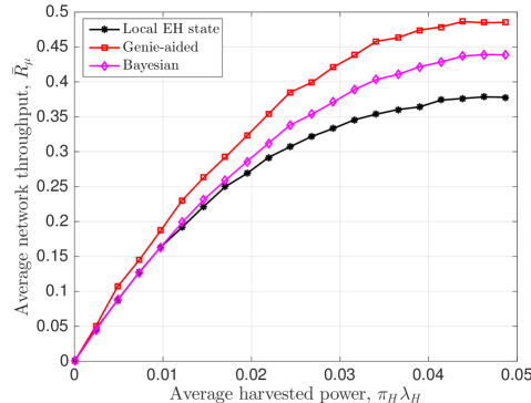
Figure 1: Network throughput vs average harvested energy per node.

In Fig. 2, we evaluate via simulation the quality of the approximations introduced by replacing the battery dynamics (2) with dynamic power constraints (3). We define an energy quantum as the quantity $P_{tx}T$, corresponding to the energy required to transmit over one slot. We assume that the EH process in the ”high” EH state is Bernoulli distributed, i.e., one energy quantum is received with probability $\lambda_{H}/P_{tx}$, otherwise no energy is received. Each transmission consumes one energy quantum. For this evaluation, we let $\lambda_{H}=\lambda_{H,\max}$. Note that the performance under ”battery dynamics” incurs a performance degradation with respect to their corresponding ”approximation”. This is a result of the fact that, when the battery dynamics are taken into account, energy outage (empty battery) and energy overflow (full battery) may occur. The degradation decreases for larger $e_{\max}$, since energy overflow becomes less significant. Nevertheless, Bayesian outperforms Local EH state by up to $20\%$, even when battery dynamics are accounted for. Thus, the approximation developed in this paper reduces significantly the optimization complexity, while preserving the goodness of the solutions. Interestingly, for large battery capacity, Local EH state evaluated under ”battery dynamics” approaches its ”approximation”, whereas a gap remains in Bayesian. This gap is due to the fact that, in Bayesian, transmissions depend on the number of active nodes $N_{H,k}$, which exhibit temporal correlation. As a result, the transmission sequence of a node also exhibits temporal correlation. This may cause larger fluctuations in the state of charge of the battery, and thus, more frequent energy outages and overflows. This effect is less relevant in Local EH state, since transmissions are independent of $N_{H,k}$.

V Conclusions

In this paper, we have considered the design of adaptive multiple access policies for LPWAN energy harvesting IoT systems. In order to reduce the complexity of network control, we have proposed an optimization framework which replaces energy storage dynamics with dynamic average power constraints induced by the time correlated energy supply. We have derived the structure of the throughput-optimal genie-aided transmission policy and, based on it, we have proposed a Bayesian estimation approach to address the more practical scenario where the number of ”active” nodes needs to be estimated based on the observed network transmission pattern. We have shown by simulation that the proposed scheme outperforms by 20% a scheme in which the nodes operate based on local state information only, and performs well even when energy storage dynamics are taken into account.

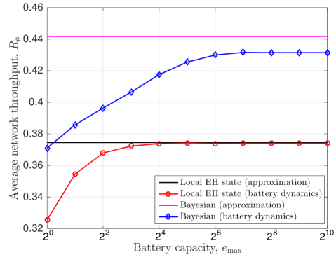
Figure 2: Network throughput vs battery capacity. ”Approximation” refers to our proposed solution which neglects battery dynamics; ”battery dynamics” is an evaluation which takes into account these dynamics.

Appendix A Proof of Theorem 1

Proof.

In order to prove this theorem, we present a general methodology. Let $\mu$ be a policy such that there exist two distinct indices $m_{1}\neq m_{2}$, $m_{1},m_{2}\in\{1,2,\dots,N\}$, such that $\mu_{H}(m_{1})<1$ and $\mu_{H}(m_{2})>0$.

Let $\mu^{(\delta)}$ be a new policy, parameterized by $\delta>0$, defined as

$$\left\{\begin{array}[]{ll}\mu^{(\delta)}_{H}(m)=\mu_{H}(m),&\forall m\notin\{m_{1},m_{2}\},\\ \mu^{(\delta)}_{H}(m_{1})=\mu_{H}(m_{1})+\delta,\\ \mu^{(\delta)}_{H}(m_{2})=\mu_{H}(m_{2})-g(\delta),\end{array}\right.$$ (42)

where $\delta>0$ is small enough to guarantee a feasible policy $\mu^{(\delta)}_{H}(m_{1})\in[0,1]$, $\mu^{(\delta)}_{H}(m_{2})\in[0,1]$, and $g(\delta)$ is a function such that the average transmission probability under $\mu$ and $\mu^{(\delta)}$ is the same, i.e.,

$$\bar{Q}_{H}(\mu)=\bar{Q}_{H}(\mu^{(\delta)}).$$ (43)

Using (42) in (III-B) and in (43), we obtain

$$g(\delta)=\frac{(m_{2}-1)!(N-m_{2})!}{(m_{1}-1)!(N-m_{1})!}\left(\frac{p_{L}}{p_{H}}\right)^{m_{2}-m_{1}}\delta.$$ (44)

Note that $g(\delta)>0$, hence $\mu^{(\delta)}$ is obtained from $\mu$ by decreasing the transmission probability in state $(H,m_{2})$, and augmenting it in state $(H,m_{1})$, in such a way as to preserve the average power consumption in the high EH state (see (43)). This is doable, since $\mu_{H}(m_{1})<1$ and $\mu_{H}(m_{2})>0$ by assumption.

Note that, if there exists $\delta>0$ (arbitrarily small) such that $\bar{R}(\mu^{(\delta)})>\bar{R}(\mu)$, then $\mu$ is strictly suboptimal and is outperformed by policy $\mu^{(\delta)}$, which thus achieves the same average power consumption as $\mu$, but strictly larger network reward. Equivalently, in the limit $\delta\to 0$, we need to verify

$$\bar{R}^{\prime}(\mu)\triangleq\lim_{\delta\to 0}\frac{\bar{R}(\mu_{\delta})-\bar{R}(\mu)}{\delta}\lessgtr 0,$$ (45)

where $\bar{R}^{\prime}(\mu)$ is the derivative of $\bar{R}(\mu_{\delta})$ with respect to $\delta$ at $0$. If $\bar{R}^{\prime}(\mu)>0$, then there exists a sufficiently small $\delta>0$ such that $\bar{R}(\mu_{\delta})>\bar{R}(\mu)$, hence $\mu$ is strictly suboptimal. On the other hand, if $\mu_{H}(m_{1})\in(0,1)$ and $\mu_{H}(m_{2})\in(0,1)$, in order for $\mu$ to be optimal, it must necessarily satisfy $\bar{R}^{\prime}(\mu)=0$; in fact, if $\bar{R}^{\prime}(\mu)>0$, then there exists a sufficiently small $\delta>0$ such that $\bar{R}(\mu_{\delta})>\bar{R}(\mu)$; in contrast, if $\bar{R}^{\prime}(\mu)<0$, then there exists a sufficiently small and negative $\delta<0$ such that $\bar{R}(\mu_{\delta})>\bar{R}(\mu)$.

Using (20), we can show that $\bar{R}^{\prime}(\mu)$ is given by

$$\bar{R}^{\prime}(\mu)$$

$${=}\!\left(\!\!\!\begin{array}[]{c}N\\ m_{1}\end{array}\!\!\!\right)\!\pi_{H}^{m_{1}}\pi_{L}^{N-m_{1}}m_{1}\!\left(1{-}\mu_{H}(m_{1})\right)^{m_{1}-2}\!\left(1{-}m_{1}\mu_{H}(m_{1})\right)$$ (48)

$${-}\!\left(\!\!\!\begin{array}[]{c}N\\ m_{2}\end{array}\!\!\!\right)\!\pi_{H}^{m_{2}}\pi_{L}^{N-m_{2}}m_{2}\!\left(1{-}\mu_{H}(m_{2})\right)^{m_{2}-2}$$ (51)

$$\qquad\qquad\times\left(1{-}m_{2}\mu_{H}(m_{2})\right)\!g^{\prime}(0)$$

$$\propto\left(1-\mu_{H}(m_{1})\right)^{m_{1}-2}\left(1-m_{1}\mu_{H}(m_{1})\right)$$

$$\quad-\left(1-\mu_{H}(m_{2})\right)^{m_{2}-2}\left(1-m_{2}\mu_{H}(m_{2})\right)$$

$$\triangleq f_{m_{1},m_{2}}(\mu_{H}(m_{1}),\mu_{H}(m_{2})),$$ (52)

where $\propto$ denotes proportionality up to a positive multiplicative factor, and $g^{\prime}(\delta)=\frac{\mathrm{d}g(\delta)}{\mathrm{d}\delta}$. Therefore, $\bar{R}^{\prime}(\mu)>0$ if and only if $f_{m_{1},m_{2}}(\mu_{H}(m_{1}),\mu_{H}(m_{2}))>0$. We use this framework to prove the structure of the optimal policy.

Case $\lambda_{H}\leq P_{tx}\pi_{L}^{N-1}$

First, we prove by contradiction that $\mu^{*}_{H}(m)=0,\forall m>1$ as in (21). Thus, let $\mu$ be a policy that does not obey this requirement, i.e., there exists $m_{2}>1$ such that $\mu_{H}(m_{2})>0$.

If $\mu_{H}(1)=1$, then $\bar{Q}_{H}(\mu)$ in (III-B) satisfies

$$\bar{Q}_{H}(\mu)=\sum_{m=0}^{N-1}\left(\!\!\!\begin{array}[]{c}N-1\\ m\end{array}\!\!\!\right)\pi_{H}^{m}\pi_{L}^{N-1-m}\mu_{H}(m+1)$$ (55)

$$=\pi_{L}^{N-1}+\left(\!\!\!\begin{array}[]{c}N-1\\ m_{2}-1\end{array}\!\!\!\right)\pi_{H}^{m_{2}-1}\pi_{L}^{N-m_{2}}\mu_{H}(m_{2})$$ (58)

$$+\sum_{m=1,m\neq m_{2}-1}^{N-1}\left(\!\!\!\begin{array}[]{c}N-1\\ m\end{array}\!\!\!\right)\pi_{H}^{m}\pi_{L}^{N-1-m}\mu_{H}(m+1)>\pi_{L}^{N-1},$$ (61)

since $\mu_{H}(m_{2})>0$. Since $\pi_{L}^{N-1}\geq\lambda_{H}/P_{tx}$ by assumption, we finally obtain

$$\bar{Q}_{H}(\mu)>\pi_{L}^{N-1}\geq\frac{\lambda_{H}}{P_{tx}},$$ (62)

and thus the constraint (5) is violated. Thus, necessarily $\mu_{H}(1)<1$ if $\mu_{H}(m_{2})>0$.

Then, let $\mu$ be such that $\mu_{H}(1)<1$ and $\mu_{H}(m_{2})>0$, for some $m_{2}>1$. Note that, letting $m_{1}=1$, we have that $\mu_{H}(m_{1})<1$ and $\mu_{H}(m_{2})>0$. Therefore, we can apply the framework developed in the preliminary part of the proof. We achieve a contradiction in the optimality of $\mu$ if $f_{m_{1},m_{2}}(\mu_{H}(m_{1}),\mu_{H}(m_{2}))>0$. Indeed, from (A) we obtain

$$f_{1,m_{2}}(\mu_{H}(1),\mu_{H}(m_{2}))$$

$$=1-(1-\mu_{H}(m_{2}))^{m_{2}-2}[1-m_{2}\mu_{H}(m_{2})],$$ (63)

which is strictly positive for $\mu_{H}(m_{2})>0$.

We thus obtain a contradiction in the optimality of $\mu_{H}$. Necessarily the optimal policy is such that $\mu_{H}^{*}(m)=0,\forall m>1$. We now optimize over $\mu_{H}^{*}(1)\in[0,1]$ to show (21). From (III-B) and (20), we have that

$$\bar{Q}_{H}(\mu^{*})=\pi_{L}^{N-1}\mu_{H}^{*}(1)\leq\frac{\lambda_{H}}{P_{tx}},$$ (64)

$$\bar{R}(\mu^{*})=N\pi_{H}\pi_{L}^{N-1}\mu_{H}^{*}(1).$$ (65)

$\bar{R}(\mu^{*})$ is an increasing function of $\mu_{H}^{*}(1)$, and thus the maximum network reward is achieved when $\bar{Q}_{H}(\mu^{*})$ is attained with equality, i.e., $\mu_{H}^{*}(1)=\frac{\lambda_{H}}{P_{tx}\pi_{L}^{N-1}}$, thus proving the optimality of (21).

Case $\lambda_{H}>P_{tx}\pi_{L}^{N-1}$

In this case, we first prove that $\mu_{H}^{*}(1)=1$. Let $\mu$ be a policy such that $\mu_{H}(1)<1$. We have two cases:

• $\mu_{H}(m)=0,\forall m>1$: in this case, we can improve the network throughput and still satisfy the (5) by setting $\mu_{H}(1)=1$, see (64)-(65).

• $\exists m_{2}>1:\mu_{H}(m_{2})>0$; as in (A), letting $m_{1}=1$, we obtain $f_{1,m_{2}}(\mu_{H}(1),\mu_{H}(m_{2}))>0$.

Thus, in both cases, such $\mu$ is strictly suboptimal. Hence, we must have $\mu_{H}^{*}(1)=1$.

We now show by contradiction that the optimal policy is such that $\mu_{H}^{*}(m)>0,\forall m>1$. Thus, let $\mu$ be a policy such that $\mu_{H}(1)=1$ and assume by contradiction that $\exists m_{1}>1:\mu_{H}(m_{1})=0$. Let $m_{2}=1$. Clearly, $m_{1}\neq m_{2}$, $0=\mu_{H}(m_{1})<1$ and $1=\mu_{H}(m_{2})>0$. Therefore, we can apply the framework developed in the preliminary part of the proof. Indeed, we have

$$f_{m_{1},m_{2}}(0,\mu_{H}(m_{2}))=f_{m_{1},1}(0,1)=1>0.$$

Therefore, $\mu$ is strictly suboptimal, hence $\mu_{H}^{*}(m){>}0,\forall m{>}1$.

We now show that $\mu_{H}^{*}(m)\leq 1/m,\forall m>1$. In fact, from (20) and (III-B) we obtain

$$\frac{\mathrm{d}\bar{R}(\mu)}{\mathrm{d}\mu_{H}(m)}=\left(\begin{array}[]{c}N\\ m\end{array}\right)\pi_{H}^{m}\pi_{L}^{N-m}m\left(1{-}\mu_{H}(m)\right)^{m-2}$$ (68)

$$\qquad\qquad\qquad\times\left(1-m\mu_{H}(m)\right),$$ (69)

$$\frac{\mathrm{d}\bar{Q}_{H}(\mu)}{\mathrm{d}\mu_{H}(m)}=\left(\begin{array}[]{c}N-1\\ m-1\end{array}\right)\pi_{H}^{m-1}\pi_{L}^{N-m}>0.$$ (72)

Note that $\bar{Q}_{H}(\mu)$ is an increasing function of $\mu_{H}(m)$, whereas $\bar{R}(\mu)$ is increasing for $\mu_{H}(m)<m^{-1}$, decreasing for $\mu_{H}(m)<m^{-1}$, and achieves the maximum at $\mu_{H}(m)=m^{-1}$. Therefore, any $\mu_{H}(m)>m^{-1}$ is suboptimal: by decreasing $\mu_{H}(m)$, one obtains a strictly larger network reward and strictly smaller average power consumption (which, thus, still satisfies the constraint (5)). Necessarily, $0<\mu_{H}^{*}(m)\leq 1/m,\forall m>1$.

Thus, let $\mu$ be a policy such that $\mu_{H}(1)=1$ and $0<\mu_{H}(m)\leq m^{-1},\forall m>1$, and let $m_{1}>m_{2}>1$. Since $\mu_{H}(m_{1})\in(0,1)$ and $\mu_{H}(m_{2})\in(0,1)$, in order to be optimal, $\mu$ needs to satisfy $f_{m_{1},m_{2}}(\mu_{H}(m_{1}),\mu_{H}(m_{2}))=0$, yielding

$$(1-\mu_{H}(m_{1}))^{m_{1}-2}[1-m_{1}\mu_{H}(m_{1})]$$

$$=(1-\mu_{H}(m_{2}))^{m_{2}-2}[1-m_{2}\mu_{H}(m_{2})],$$

for all pairs $m_{1}>m_{2}>1$, and therefore we obtain (23), repeated here for convenience,

$$\left(1-\mu_{H}(m)\right)^{m-2}\left(1-m\mu_{H}(m)\right)=\phi,\ \forall m>1,$$ (73)

where $\phi\in[0,1)$ is a constant (note that, since $\mu_{H}(m)>0$, necessarily $\phi<1$). The left hand side of (73) is a strictly decreasing function of $\mu_{H}(m)\in(0,m^{-1})$, which equals $1$ for $\mu_{H}(m)=0$ and $0$ for $\mu_{H}(m)=1/m$. Therefore, there exists a unique $\mu_{H}(m)\in(0,1/m]$, denoted as $\mu_{H}^{(\phi)}(m)$, which satisfies (73) with equality.

Thus, it remains to prove that the optimal policy is given by $\mu_{H}^{*}(1)=1$, $\mu_{H}^{*}(m)=\mu_{H}^{(\phi)}(m),\forall m>1$, for some $\phi\in[0,1)$. To conclude, we need to determine such $\phi$.

Since the left hand side of (73) is a strictly decreasing function of $\mu_{H}(m)\in(0,m^{-1})$, it follows that $\mu_{H}^{(\phi)}(m)$ is a strictly decreasing function of $\phi$, with $\mu_{H}^{(0)}(m)=m^{-1}$ and $\lim_{\phi\to 1}\mu_{H}^{(\phi)}(m)=0$. Therefore, for $1>\phi_{1}>\phi_{2}\geq 0$, we get $\mu_{H}^{(\phi_{1})}(m)<\mu_{H}^{(\phi_{2})}(m),\forall m>1$, hence, by inspection of (III-B), we obtain

$$\bar{Q}(\mu^{(\phi_{1})})<\bar{Q}(\mu^{(\phi_{2})}).$$ (74)

Similarly, since $\bar{R}(\mu)$ is an increasing function of $\mu_{H}(m)\in(0,m^{-1}),\forall m>1$, by inspection of (20) we obtain

$$\bar{R}(\mu^{(\phi_{1})})<\bar{R}(\mu^{(\phi_{2})}).$$ (75)

Hence, $\bar{R}(\mu^{(\phi)})$ and $\bar{Q}(\mu^{(\phi)})$ are strictly decreasing functions of $\phi\in[0,1)$. When $\phi=0$, we obtain $\mu_{H}^{(0)}(m)=m^{-1}$, hence

$$\bar{Q}_{H}(\mu^{(0)})=\sum_{m=0}^{N-1}\left(\begin{array}[]{c}N-1\\ m\end{array}\right)\pi_{H}^{m}\pi_{L}^{N-1-m}\frac{1}{m+1}$$ (78)

$$=\frac{1}{N\pi_{H}}\sum_{m=1}^{N}\left(\begin{array}[]{c}N\\ m\end{array}\right)\pi_{H}^{m}\pi_{L}^{N-m}$$ (81)

$$=\frac{(\pi_{H}+\pi_{L})^{N}-\pi_{L}^{N}}{N\pi_{H}}=\frac{\lambda_{H,\max}}{P_{tx}},$$ (82)

where we have used the fact that $\pi_{H}+\pi_{L}=1$, and the definition of $\lambda_{H,\max}$.

Therefore, when $\lambda_{H}\geq\lambda_{H,\max}$, from (74) and (75), for all $\phi\in[0,1)$ we obtain

$$\bar{R}(\mu^{(\phi)})\leq\bar{R}(\mu^{(0)}),$$ (83)

$$\bar{Q}(\mu^{(\phi)})\leq\bar{Q}(\mu^{(0)})=\frac{\lambda_{H,\max}}{P_{tx}}\leq\frac{\lambda_{H}}{P_{tx}}.$$ (84)

Clearly, $\mu^{(0)}$ satisfies the constraint (5) and achieves the maximum network reward over $\phi\in[0,1)$. Hence, the policy $\mu_{H}^{(0)}(m)=m^{-1}$ is optimal when $\lambda_{H}\geq\lambda_{H,\max}$, thus proving (24).

On the other hand, when $\lambda_{H}<\lambda_{H,\max}$, policy $\mu_{H}^{(0)}(m)$ violates the constraint (5). Necessarily, in this case $0<\phi<1$. Note that, in the limit $\phi\to 1$, we obtain $\mu_{H}^{(1)}(m)=0,\forall m>1$, hence $\lim_{\phi\to 1}\bar{Q}(\mu^{(\phi)})=\pi_{L}^{N-1}$. Thus, $\forall\phi\in(0,1)$ we obtain

$$\pi_{L}^{N-1}=\lim_{\phi\to 1}\bar{Q}(\mu^{(\phi)})<\bar{Q}(\mu^{(\phi)})<\bar{Q}(\mu^{(0)})=\frac{\lambda_{H,\max}}{P_{tx}},$$

and, by assumption,

$$\pi_{L}^{N-1}<\frac{\lambda_{H}}{P_{tx}}<\frac{\lambda_{H,\max}}{P_{tx}}.$$ (85)

Therefore, there exists a unique $\hat{\phi}\in(0,1)$ such that $\bar{Q}(\mu^{(\hat{\phi})})=\frac{\lambda_{H}}{P_{tx}}$. Under such $\hat{\phi}$, we obtain

$$\left\{\begin{array}[]{l}\bar{R}(\mu^{(\phi)})<\bar{R}(\mu^{(\hat{\phi})}),\\ \bar{Q}(\mu^{(\phi)})<\bar{Q}(\mu^{(\hat{\phi})})=\frac{\lambda_{H}}{P_{tx}},\end{array}\right.\ \forall 0<\phi<\hat{\phi},$$ (88)

and

$$\bar{Q}(\mu^{(\phi)})>\bar{Q}(\mu^{(\hat{\phi})})=\frac{\lambda_{H}}{P_{tx}},\ \forall\hat{\phi}<\phi<1.$$ (89)

We conclude that any $\phi>\hat{\phi}$ violates the constraint, whereas any $\phi<\hat{\phi}$ is strictly suboptimal. Thus, $\hat{\phi}$ is the optimal value among $\phi\in(0,1)$ which maximizes the network reward under the constraint (5).

The theorem is thus proved. ∎

Appendix B Proof of Theorem 2

Proof.

Assume node $n$ is in the ”high” EH state in slot $k$. Then, the expected transmission probability satisfies

$$\mathbb{E}\left[q_{n,k}|S_{n,k}=H\right]=\mathbb{P}\left(q_{n,k}=1|S_{n,k}=H\right)$$

$$=\sum_{\mathbf{t}}\mathbb{P}\left(q_{n,k}=1,\mathbf{t}_{k}=\mathbf{t}|S_{n,k}=H\right),$$ (90)

where $\mathbf{t}_{k}{=}(t_{0},t_{1},\dots,t_{k-1})\in\{0,1,\dots,N\}^{k}$ is the vector of nodes that transmit from slot $0$ to slot $k-1$. Then, using Bayes’ rule,

$$\mathbb{P}\left(q_{n,k}{=}1,\mathbf{t}_{k}{=}\mathbf{t}|S_{n,k}{=}H\right)=\mathbb{P}\left(q_{n,k}{=}1|\mathbf{t}_{k}{=}\mathbf{t},S_{n,k}{=}H\right)$$

$$\qquad\times\frac{\mathbb{P}\left(S_{n,k}=H|\mathbf{t}_{k}=\mathbf{t}\right)\mathbb{P}\left(\mathbf{t}_{k}=\mathbf{t}\right)}{\mathbb{P}(S_{n,k}=H)}.$$ (91)

Note that the belief in slot $k$ available at the gateway is a function of $\mathbf{t}_{k}$, as can be seen from (25). This can be proved by induction. In fact, $\beta_{0}(m)=\mathbb{P}(N_{H,0}=m)$ (prior at time $0$), $\mu_{0}$ is a function of $\beta_{0}$ via (37), and $\beta_{1}$ is a function of $(\beta_{0},\mu_{0},t_{0})$ via (III-C); thus, $\beta_{1}$ is a function of $t_{0}$. Then, assuming that $\beta_{k-1}$ is a function of $\mathbf{t}_{k-1}$, we have the following: $\mu_{k-1}$ is a function of $\beta_{k-1}$ via (37), and $\beta_{k}$ is a function of $(\beta_{k-1},\mu_{k-1},t_{k-1})$ via (III-C); thus, $\beta_{k}$ is a function of $\mathbf{t}_{k}=(\mathbf{t}_{k-1},t_{k-1})$, and by induction $\beta_{k}$ is a function of $\mathbf{t}_{k}$, for all $k\geq 0$. We denote this function as $\beta_{k}(m)=\psi_{k}(m|\mathbf{t}_{k})$, and we denote (37) computed under such $\mathbf{t}_{k}$ as $\mu_{k}(\mathbf{t}_{k})$. It follows that

$$\mathbb{P}\left(q_{n,k}=1|\mathbf{t}_{k}=\mathbf{t},S_{n,k}=H\right)=\mu_{k}(\mathbf{t})$$

$$=\frac{\sum_{m=1}^{N}\psi_{k}(m|\mathbf{t})m\mu_{H}^{*}(m)}{\sum_{m=1}^{N}\psi_{k}(m|\mathbf{t})m}.$$ (92)

Additionally,

$$\mathbb{P}\left(S_{n,k}=H|\mathbf{t}_{k}=\mathbf{t}\right)=\sum_{m=1}^{N}\mathbb{P}\left(S_{n,k}{=}H,N_{H,k}{=}m|\mathbf{t}_{k}{=}\mathbf{t}\right)$$

$$\!\!\!\!=\!\!\sum_{m=1}^{N}\mathbb{P}\left(S_{n,k}{=}H|N_{H,k}{=}m,\mathbf{t}_{k}{=}\mathbf{t}\right)\mathbb{P}\left(N_{H,k}{=}m|\mathbf{t}_{k}{=}\mathbf{t}\right),$$ (93)

where we have marginalized with respect to the number of active nodes $N_{H,k}$ (clearly, $N_{H,k}>0$ since $S_{n,k}=H$). Note that, independently of $\mathbf{t}_{k}$, when $N_{H,k}=m$ nodes are active, the probability that $S_{n,k}=H$ is $m/N$. In fact, nodes are identical to each other. We thus obtain

$$\mathbb{P}\left(S_{n,k}=H|\mathbf{t}_{k}=\mathbf{t}\right)=\frac{1}{N}\sum_{m=1}^{N}m\mathbb{P}\left(N_{H,k}{=}m|\mathbf{t}_{k}{=}\mathbf{t}\right)$$

$$=\frac{1}{N}\sum_{m=1}^{N}m\psi_{k}(m|\mathbf{t}),$$ (94)

where the second step follows from the definition of $\psi_{k}(m|\mathbf{t})$. By replacing (B) and (B) into (B), we thus obtain

$$\mathbb{P}\left(q_{n,k}{=}1,\mathbf{t}_{k}{=}\mathbf{t}|S_{n,k}{=}H\right)$$

$$=\frac{1}{N\mathbb{P}(S_{n,k}=H)}\sum_{m=1}^{N}\psi_{k}(m|\mathbf{t})\mathbb{P}\left(\mathbf{t}_{k}{=}\mathbf{t}\right)m\mu_{H}^{*}(m)$$

$$=\frac{1}{N\mathbb{P}(S_{n,k}=H)}\sum_{m=1}^{N}\mathbb{P}\left(N_{H,k}{=}m,\mathbf{t}_{k}{=}\mathbf{t}\right)m\mu_{H}^{*}(m),$$ (95)

where in the last step we have used the definition of $\psi_{k}(m|\mathbf{t})$. Finally, by replacing (B) into (B), we obtain

$$\mathbb{E}\left[q_{n,k}|S_{n,k}=H\right]$$

$$=\frac{1}{N\mathbb{P}(S_{n,k}=H)}\sum_{m=1}^{N}\mathbb{P}\left(N_{H,k}{=}m\right)m\mu_{H}^{*}(m),$$ (96)

where we have marginalized with respect to $\mathbf{t}_{k}$.

On the other hand, with the genie-aided scheme, we obtain

$$\mathbb{E}\left[q_{n,k}|S_{n,k}=H\right]=\mathbb{P}\left(q_{n,k}=1|S_{n,k}=H\right)$$

$$=\sum_{m=1}^{N}\mathbb{P}\left(q_{n,k}=1|N_{H,k}=m,S_{n,k}=H\right)$$

$$\quad\times\frac{\mathbb{P}\left(S_{n,k}=H|N_{H,k}=m\right)\mathbb{P}\left(N_{H,k}=m\right)}{\mathbb{P}(S_{n,k}=H)},$$ (97)

where we have marginalized with respect to $N_{H,k}$ and used Bayes’ rule. Note that, in the genie-aided scheme, $\mathbb{P}\left(q_{n,k}=1|N_{H,k}=m,S_{n,k}=H\right)=\mu_{H}^{*}(m)$. Additionally, $\mathbb{P}\left(S_{n,k}=H|N_{H,k}=m\right)=m/N$, since nodes are identical. Thus, we finally obtain

$$\mathbb{E}\left[q_{n,k}|S_{n,k}=H\right]$$

$$=\frac{1}{N\mathbb{P}(S_{n,k}=H)}\sum_{m=1}^{N}\mathbb{P}\left(N_{H,k}{=}m\right)m\mu_{H}^{*}(m),$$ (98)

which is the same expression as (B) for the Bayesian case.

We conclude that, in every slot, the expected transmission probability (hence the expected power consumption) is the same under the genie-aided and Bayesian schemes. The theorem is proved. ∎

Appendix C Bisection algorithms

We now present two bisection algorithms, to compute the value of $\phi\in(0,1)$ in Theorem 1, and to compute the $\mu_{H}(m)$ for a given $\phi$ in (23), respectively. To this end, note from the proof of Theorem 1 in Appendix A that $\bar{Q}(\mu^{(\phi)})$ and $\bar{R}(\mu^{(\phi)})$ are strictly decreasing functions of $\phi$, see (74) and (75). It follows that, if $\bar{Q}_{H}(\mu^{(\tilde{\phi})})<\min\left\{1,\frac{\lambda_{H}}{P_{tx}}\right\}$, then $\phi>\tilde{\phi}$ and $\tilde{\phi}$ is a lower bound to $\phi$; vice versa, if $\bar{Q}_{H}(\mu^{(\tilde{\phi})})>\min\left\{1,\frac{\lambda_{H}}{P_{tx}}\right\}$, then $\phi<\tilde{\phi}$ and $\tilde{\phi}$ is an upper bound to $\phi$. This observation leads to the following bisection algorithm.

Algorithm 1.

[To determine $\phi$ in Theorem 1]

• Init: $\phi_{\min}=0$, $\phi_{\max}=1$; accuracy $\epsilon_{\phi}\ll 1$;

• Main: $\tilde{\phi}:=\frac{\phi_{\min}+\phi_{\max}}{2}$. Determine $\tilde{\mu}_{H}$ via Algorithm 2; if $\bar{Q}_{H}(\tilde{\mu}_{H}){<}\min\left\{1,\frac{\lambda_{H}}{P_{tx}}\right\}$, set $\phi_{\min}{:=}\tilde{\phi}$; otherwise, set $\phi_{\max}{:=}\tilde{\phi}$;

• Test: repeat Main until $\phi_{\max}-\phi_{\min}<\epsilon_{\phi}$; finally, return $\phi=\frac{\phi_{\min}+\phi_{\max}}{2}$.

For a given $\tilde{\phi}$ in Algorithm 1, we leverage the fact that the right hand expression of (23) is a decreasing function of $\mu_{H}(m)\in(0,1/m)$. This observation leads to the following bisection algorithm.

Algorithm 2.

[To find $\tilde{\mu}_{H}$ given $\tilde{\phi}$] $\forall m\in\{2,3,\dots,N\}$:

• Init: $\tilde{\phi}$ given; $u_{\min}{=}0$, $u_{\max}{=}1/m$; accuracy $\epsilon_{\mu}{\ll}1$;

• Main: $\tilde{u}{:=}\frac{u_{\min}+u_{\max}}{2}$. If $(1{-}\tilde{u})^{m-2}(1{-}m\tilde{u}){>}\tilde{\phi}$, set $u_{\min}:=\tilde{u}$; otherwise, set $u_{\max}:=\tilde{u}s$;

• Test: repeat Main until $u_{\max}-u_{\min}<\epsilon_{\mu}$; finally, return $\tilde{\mu}_{H}(m)=\frac{u_{\min}+u_{\max}}{2}$.

References

• [1] A. Zanella, N. Bui, A. Castellani, L. Vangelista, and M. Zorzi, “Internet of things for smart cities,” IEEE Internet of Things Journal, vol. 1, no. 1, pp. 22–32, 2014.
• [2] “LoRaWANTM Specification,” Tech. Rep., July 2016, version V1.0.2. [Online]. Available: https://www.lora-alliance.org
• [3] L. Vangelista, A. Zanella, and M. Zorzi, “Long-Range IoT Technologies: The Dawn of LoRa?” in Future Access Enablers of Ubiquitous and Intelligent Infrastructures.   Springer, 2015, pp. 51–58.
• [4] M. Centenaro, L. Vangelista, A. Zanella, and M. Zorzi, “Long-range communications in unlicensed bands: the rising stars in the IoT and smart city scenarios,” IEEE Wireless Communications, vol. 23, no. 5, pp. 60–67, October 2016.
• [5] J. A. Paradiso and T. Starner, “Energy scavenging for mobile and wireless electronics,” IEEE Pervasive Computing, vol. 4, no. 1, pp. 18–27, Jan 2005.
• [6] D. Gunduz, K. Stamatiou, N. Michelusi, and M. Zorzi, “Designing intelligent energy harvesting communication systems,” IEEE Communications Magazine, vol. 52, no. 1, pp. 210–216, January 2014.
• [7] P. Kamalinejad, C. Mahapatra, Z. Sheng, S. Mirabbasi, V. C. Leung, and Y. L. Guan, “Wireless energy harvesting for the internet of things,” IEEE Communications Magazine, vol. 53, no. 6, pp. 102–108, 2015.
• [8] N. Michelusi, L. Badia, and M. Zorzi, “Optimal Transmission Policies for Energy Harvesting Devices With Limited State-of-Charge Knowledge,” IEEE Transactions on Communications, vol. 62, no. 11, pp. 3969–3982, Nov 2014.
• [9] R. Valentini and M. Levorato, “Optimal aging-aware channel access control for wireless networks with energy harvesting,” in 2016 IEEE International Symposium on Information Theory (ISIT).   IEEE, 2016, pp. 2754–2758.
• [10] R. Valentini, M. Levorato, and F. Santucci, “Aging aware random channel access for battery-powered wireless networks,” IEEE Wireless Communications Letters, vol. 5, no. 2, pp. 176–179, 2016.
• [11] N. Michelusi, K. Stamatiou, and M. Zorzi, “Transmission Policies for Energy Harvesting Sensors with Time-Correlated Energy Supply,” IEEE Transactions on Communications, vol. 61, no. 7, pp. 2988–3001, July 2013.
• [12] D. D. Testa, N. Michelusi, and M. Zorzi, “Optimal transmission policies for two-user energy harvesting device networks with limited state-of-charge knowledge,” IEEE Transactions on Wireless Communications, vol. 15, no. 2, pp. 1393–1405, Feb 2016.
• [13] M. Gatzianas, L. Georgiadis, and L. Tassiulas, “Control of wireless networks with rechargeable batteries,” IEEE Transactions on Wireless Communications, vol. 9, no. 2, pp. 581–593, February 2010.
• [14] B. Varan and A. Yener, “Delay constrained energy harvesting networks with limited energy and data storage,” IEEE Journal on Selected Areas in Communications, vol. 34, no. 5, pp. 1550–1564, May 2016.
• [15] S. Ulukus, A. Yener, E. Erkip, O. Simeone, M. Zorzi, P. Grover, and K. Huang, “Energy Harvesting Wireless Communications: A Review of Recent Advances,” IEEE Journal on Selected Areas in Communications, vol. 33, no. 3, pp. 360–381, March 2015.
• [16] N. Michelusi and M. Zorzi, “Optimal Adaptive Random Multiaccess in Energy Harvesting Wireless Sensor Networks,” IEEE Transactions on Communications, vol. 63, no. 4, pp. 1355–1372, April 2015.
• [17] K. S. Gilhousen, I. M. Jacobs, R. Padovani, A. J. Viterbi, L. A. Weaver, and C. E. Wheatley, “On the capacity of a cellular cdma system,” IEEE Transactions on Vehicular Technology, vol. 40, no. 2, pp. 303–312, May 1991.
• [18] R. L. Burden and J. D. Faires, Numerical Analysis, 9th Edition.   Cengage Learning, 2011.
• [19] E. J. Sondik, “The Optimal Control of Partially Observable Markov Processes over the Infinite Horizon: Discounted Costs,” Oper. Res., vol. 26, no. 2, pp. 282–304, Apr. 1978.