Wobbling motion in ¹³⁵Pr within a collective Hamiltonian

Abstract

The recently reported wobbling bands in ¹³⁵Pr are investigated by the collective Hamiltonian, in which the collective parameters, including the collective potential and the mass parameter, are respectively determined from the tilted axis cranking (TAC) model and the harmonic frozen alignment (HFA) formula. It is shown that the experimental energy spectra of both yrast and wobbling bands are well reproduced by the collective Hamiltonian. It is confirmed that the wobbling mode in ¹³⁵Pr changes from transverse to longitudinal with the rotational frequency. The mechanism of this transition is revealed by analyzing the effective moments of inertia of the three principal axes, and the corresponding variation trend of the wobbling frequency is determined by the softness and shapes of the collective potential.

I Introduction

The triaxial shape has been a long-standing subject in nuclear physics. The appearance of the wobbling bands Bohr and Mottelson (1975); Odegaard et al. (2001) and the chiral doublet bands Frauendorf and Meng (1997); Starosta et al. (2001) has provided unambiguous experimental evidence of triaxiality. The wobbling mode was first proposed by Bohr and Mottelson in the 1970s Bohr and Mottelson (1975). It exists in a triaxial nucleus when the total spin of the nucleus does not align along any of the principal axes, but precesses and wobbles around one of the axes, in analogy to an asymmetric deformed top Landau and Lifshitz (1960).

The wobbling bands were first observed in ¹⁶³Lu Odegaard et al. (2001); Jensen et al. (2002). Since then, seven more wobbling nuclei have been reported, including ¹⁶¹Lu Bringel et al. (2005), ¹⁶⁵Lu Schönwaßer et al. (2003), ¹⁶⁷Lu Amro et al. (2003), and ¹⁶⁷Ta Hartley et al. (2009) in $A\sim 160$, ¹³⁵Pr Matta et al. (2015) in $A\sim 130$, and even-even ¹¹²Ru Zhu et al. (2009) and ¹¹⁴Pd Luo et al. (2013) in the $A\sim 110$ mass regions. Among the odd-$A$ wobblers, ¹³⁵Pr is the only one out of the $A\sim 160$ mass region, which is built on a proton $h_{11/2}$ configuration with a moderate deformation ($\beta\sim 0.17$), while the others in $A\sim 160$ involve a proton $i_{13/2}$ configuration with significantly large deformation ($\beta\sim 0.40$).

The excitation energy of a wobbling motion is characterized by wobbling frequency. In the originally predicted wobbler for a pure triaxial rotor (simple wobbler) Bohr and Mottelson (1975), the wobbling frequency increases with spin. However, decreasing wobbling frequencies with spin were observed in the Lu and Ta isotopes as shown in Ref. Hartley et al. (2011). To clarify this contradiction, Frauendorf and Dönau Frauendorf and Dönau (2014) distinguished two types of wobbling motions, longitudinal and transverse wobblers, for a triaxial rotor coupled with a high-$j$ quasiparticle. For the longitudinal wobbler, the quasiparticle angular momentum and the principal axis with the largest moment of inertia (MOI) are parallel; for the transverse one, they are perpendicular. They demonstrated that the wobbling frequency of a longitudinal wobbler increases with spin, while that of a transverse one decreases with spin Frauendorf and Dönau (2014). Therefore, the wobbling bands in the Lu and Ta isotopes are interpreted as transverse wobbling bands.

Theoretically, the triaxial particle rotor model (PRM) Bohr and Mottelson (1975); Hamamoto (2002); Hamamoto and Mottelson (2003); Tanabe and Sugawara-Tanabe (2006, 2008); Sugawara-Tanabe and Tanabe (2010); Sugawara-Tanabe et al. (2014); Frauendorf and Dönau (2014); Shi and Chen (2015) and the cranking model plus random phase approximation (RPA) Marshalek (1979); Shimizu and Matsuzaki (1995); Matsuzaki et al. (2002); Matsuzaki et al. (2004a, b); Matsuzaki and Ohtsubo (2004); Shimizu et al. (2005, 2008); Shoji and Shimizu (2009); Frauendorf and Dönau (2015) have been widely used to describe the wobbling motion. Recently, based on the cranking mean field and treating the nuclear orientation as collective degree of freedom, a collective Hamiltonian was constructed and applied for the chiral Chen et al. (2013) and wobbling modes Chen et al. (2014). Usually, the orientation of a nucleus in the rotating mean field is described by the polar angle $\theta$ and azimuth angle $\varphi$ in spherical coordinates. In the collective Hamiltonian for wobbling modes, the azimuth angle $\varphi$ is taken as the collective coordinate since the motion along the $\varphi$ direction is much easier than in the $\theta$ direction Chen et al. (2014). The quantum fluctuations along $\varphi$ are taken into account to go beyond the mean-field approximation. Using this model, the simple, longitudinal, and transverse wobblers were systematically studied and the variation trends of their wobbling frequencies were confirmed Chen et al. (2014).

With the successes of the collective Hamiltonian, it is interesting to extend its applications. In ¹³⁵Pr Matta et al. (2015), not only the transverse wobbling mode, but also its transition to the longitudinal wobbling were observed. The experimental observations have already been investigated by tilted axis cranking (TAC) with the Strutinsky micro-macro method and the PRM in Ref. Matta et al. (2015). Here the collective Hamiltonian will be applied to investigate the wobbling motions in ¹³⁵Pr.

II Theoretical framework

The adopted collective Hamiltonian was introduced in detail in Refs. Chen et al. (2013, 2014). Choosing the azimuth angle $\varphi$ as the collective coordinate, the collective Hamiltonian reads

$$\hat{H}_{\rm coll}=-\displaystyle\frac{\hbar^{2}}{2\sqrt{B(\varphi)}}\frac{\partial}{\partial\varphi}\frac{1}{\sqrt{B(\varphi)}}\frac{\partial}{\partial\varphi}+V(\varphi),$$ (1)

where the collective potential $V(\varphi)$ is extracted by minimizing the total Routhian $E^{\prime}(\theta,\varphi)$ of TAC calculations with respect to the polar angle $\theta$ for given $\varphi$ Chen et al. (2013, 2014). For a high-$j$, the TAC Hamiltonian reads Frauendorf and Meng (1997)

$$\hat{h}^{\prime} =\hat{h}_{\rm def}-\bm{\omega}\cdot\hat{\bm{j}},$$

$$\bm{\omega} =(\omega\sin\theta\cos\varphi,\omega\sin\theta\sin\varphi,\omega\cos\theta),$$ (2)

where $\hat{\bm{j}}$ is the single particle angular momentum and $\hat{h}_{\rm def}$ is the single-$j$ shell Hamiltonian,

$$\hat{h}_{\rm def}=\frac{1}{2}C\Big{\{}(\hat{j}_{3}^{2}-\frac{j(j+1)}{3})\cos\gamma+\frac{1}{2\sqrt{3}}(\hat{j}_{+}^{2}+\hat{j}_{-}^{2})\sin\gamma\Big{\}}.$$ (3)

In Eq. (3), the parameter $C$ is proportional to the quadrupole deformation parameter $\beta$, and $\gamma$ is triaxial deformation parameter. Diagonalizing the cranking Hamiltonian, one ends up with the total Routhian

$$E^{\prime}(\theta,\varphi)=\langle h^{\prime}\rangle-\frac{1}{2}\sum_{k=1}^{3}\mathcal{J}_{k}\omega_{k}^{2},\quad\mathcal{J}_{k}:\textrm{moments of inertia},$$ (4)

and then the collective potential $V(\varphi)$.

To obtain the mass parameter, one can expand the collective potential $V(\varphi)$ with respect to $\varphi$ at $\varphi=0^{\circ}$ up to $\sim\varphi^{2}$ terms to extract the stiffness parameter (labeled $K$) of $V(\varphi)$ Chen et al. (2014), and then

$$B=\frac{K}{\Omega^{2}}$$ (5)

with $\Omega$ the wobbling frequency. For example, for a simple wobbler, its stiffness parameter is $K=\omega^{2}(\mathcal{J}_{1}-\mathcal{J}_{2})$ Chen et al. (2014), and its wobbling frequency can be calculated by the triaxial rotor model: Bohr and Mottelson (1975)

$$\hbar\Omega=\hbar\omega\sqrt{\frac{(\mathcal{J}_{1}-\mathcal{J}_{2})(\mathcal{J}_{1}-\mathcal{J}_{3})}{\mathcal{J}_{3}\mathcal{J}_{2}}},$$ (6)

with $\omega$ the rotational frequency. Thus, according to Eq. (5), the mass parameter is Chen et al. (2014)

$$B=\frac{\mathcal{J}_{2}\mathcal{J}_{3}}{\mathcal{J}_{1}-\mathcal{J}_{3}}.$$ (7)

For an odd-$A$ wobbler, one further introduces the harmonic frozen alignment (HFA) approximation Frauendorf and Dönau (2014, 2015); i.e., the odd particle is assumed to be firmly aligned with axis 1 (see left panel of Fig. 1), and its angular momentum is considered as a constant number $j$. Such an assumption leads to an $\omega$-dependent effective MOI for axis 1 with $j/\omega$. Therefore, the Eq. (7) is replaced by Chen et al. (2014)

$$B(\omega)=\frac{\mathcal{J}_{2}\mathcal{J}_{3}}{\mathcal{J}_{1}^{*}(\omega)-\mathcal{J}_{3}},\quad\mathcal{J}_{1}^{*}(\omega)=\mathcal{J}_{1}+\frac{j}{\omega}.$$ (8)

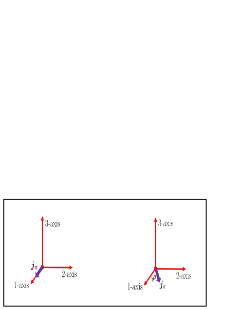
Figure 1: (Color online) Sketch of the angular momentum vector of the proton particle with respect to the principal axis frame.

If the angular momentum of the odd particle tilts from axis 1 toward axis 2, as illustrated in the right panel of Fig. 1, the effective MOI induced should be modified accordingly. If the tilted angle is $\varphi$, the effective MOIs for axes 1 and 2 are

$$\mathcal{J}_{1}^{*}(\omega) =\mathcal{J}_{1}+\frac{j\cos\varphi}{\omega},$$ (9)

$$\mathcal{J}_{2}^{*}(\omega) =\mathcal{J}_{2}+\frac{j\sin\varphi}{\omega}.$$ (10)

Correspondingly, the mass parameter (8) should be rewritten as

$$B(\omega)=\frac{\mathcal{J}_{2}^{*}(\omega)\mathcal{J}_{3}}{\mathcal{J}_{1}^{*}(\omega)-\mathcal{J}_{3}}.$$ (11)

With the collective potential from the TAC model Chen et al. (2013, 2014) and the mass parameter from the HFA formula (11), the collective Hamiltonian (1) is constructed. Similar to Refs. Chen et al. (2013, 2014), the collective Hamiltonian is solved by diagonalization. Since the collective Hamiltonian is invariant with respect to the $\varphi\to-\varphi$ transformation, one chooses the following bases

$$\psi_{n}^{(1)}(\varphi) =\sqrt{\frac{2}{\pi(1+\delta_{n0})}}\frac{\cos 2n\varphi}{B^{1/4}(\omega)},\quad n\geq 0,$$ (12)

$$\psi_{n}^{(2)}(\varphi) =\sqrt{\frac{2}{\pi}}\frac{\sin 2n\varphi}{B^{1/4}(\omega)},\quad n\geq 1,$$ (13)

which satisfy

$$\psi_{n}^{(1)}(-\varphi)=\psi_{n}^{(1)}(\varphi),\quad\psi_{n}^{(2)}(-\varphi)=-\psi_{n}^{(2)}(\varphi),$$ (14)

and the periodic boundary condition as

$$\psi_{n}^{(1)}(\varphi)=\psi_{n}^{(1)}(\varphi+\pi),\quad\psi_{n}^{(2)}(\varphi)=\psi_{n}^{(2)}(\varphi+\pi).$$ (15)

III Numerical details

In the following calculations, the configuration of the wobbling bands in ¹³⁵Pr is adopted as $\pi(1h_{11/2})^{1}$. The quadrupole deformation parameters follow Refs. Frauendorf and Dönau (2014); Matta et al. (2015) as $\beta=0.17$ and $\gamma=-26.0^{\circ}$. Accordingly, the axes 1, 2, and 3 are respectively the short, intermediate, and long axes. The MOIs for the three principal axes are taken as $\mathcal{J}_{1}$, $\mathcal{J}_{2}$, $\mathcal{J}_{3}$=13.0, 21.0, 4.0 $\hbar^{2}/\rm{MeV}$ Frauendorf and Dönau (2014). It is seen that all the parameters are the same as in previous works Frauendorf and Dönau (2014); Matta et al. (2015), and no adjustable parameters are introduced in the present calculations.

IV Results and discussion

In a recent reported transverse wobbling partners in the $A\sim 130$ mass region, ¹³⁵Pr, the wobbling frequency decreases with spin, and the $\Delta I=1$ interband transitions between the partner bands display primarily $E2$ character Matta et al. (2015). In Refs. Matta et al. (2015); Frauendorf and Dönau (2014), the TAC Strutinsky micro-macro calculations adopt the deformation parameters $\beta=0.17$ and $\gamma=-26.0^{\circ}$ and the PRM (or so-called quasiparticle triaxial rotor model) adopts the MOIs as $\mathcal{J}_{1}$, $\mathcal{J}_{2}$, $\mathcal{J}_{3}$=13.0, 21.0, 4.0 $\hbar^{2}/\rm{MeV}$, respectively. In the present collective Hamiltonian calculations, we also use the same parameters Matta et al. (2015); Frauendorf and Dönau (2014), and no additional parameters.

The total Routhian surfaces $E^{\prime}(\theta,\varphi)$ calculated by the TAC model for ¹³⁵Pr at the rotational frequencies $\hbar\omega=0.10$, $0.30$, $0.50$, and $0.70~{}\rm MeV$ are shown in Fig. 2, where the minima are labeled with red stars. It can be seen that all the total Routhian surfaces are symmetric with respect to the $\varphi=0^{\circ}$ and $\theta=90^{\circ}$ lines, as a result of the invariance of the intrinsic quadrupole moments with respect to the $D_{2}$ symmetry.

It is shown that the $\theta$ values of the minima always locate at $\theta=90^{\circ}$. This is because axis 3 is of the smallest MOI and, as a consequence, the angular momentum prefers to align in the 1-2 plane. With the increase of rotational frequency, the $\varphi$ values of the minima gradually deviate from a vanishing value to finite angles. As a result, the number of the minima changes from one to two. This implies the rotational mode changes from a principal axis rotation at low frequencies (e.g., $\hbar\omega=0.10$ and $0.30$ MeV) to a planar rotation at high frequencies (e.g., $\hbar\omega=0.70$ and $0.90$ MeV). These features provide a hint of the existence of the transverse wobbling mode Chen et al. (2014).

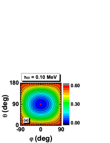
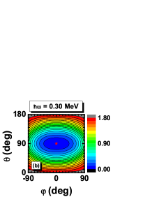
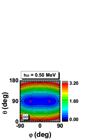
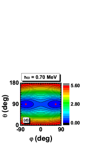
Figure 2: (Color online) Contour plots of the total Routhian surface calculation $E^{\prime}(\theta,\varphi)$ for ¹³⁵Pr at the frequencies $\hbar\omega=0.10$, $0.30$, $0.50$, and $0.70~{}\rm MeV$. All energies at each rotational frequency are normalized with respect to the absolute minimum.

To see more clearly, $\varphi_{\min}$, i.e., the $\varphi$ which minimizes the total Routhian surface, is shown in Fig. 3 as a function of rotational frequency. $\varphi_{\min}$ is zero below $\hbar\omega=0.40~{}\mathrm{MeV}$, and is bifurcate above this rotational frequency. Thus $\hbar\omega=0.40~{}\mathrm{MeV}$ is the critical rotational frequency at which the rotational mode changes. For $\hbar\omega>0.40~{}\mathrm{MeV}$, $\varphi_{\min}$ gradually deviates from zero and, at $\hbar\omega=0.70~{}\rm{MeV}$, reaches $\sim\pm 65^{\circ}$. It is expected that it would approach to $\pm 90^{\circ}$ with the increasing rotational frequency. In that case, the rotational mode changes from a planar rotation to a principal axis rotation around axis 2.

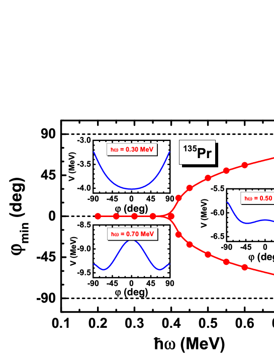
Figure 3: (Color online) $\varphi_{\min}$, i.e., the $\varphi$ which minimizes the total Routhian surface, as a function of rotational frequency and the extracted collective potential $V(\varphi)$ at $\hbar\omega=0.30$, $0.50$, and $0.70~{}\rm{MeV}$.

In Fig. 3, we also show the collective potential $V(\varphi)$ obtained by minimizing the total Routhian $E^{\prime}(\theta,\varphi)$ with respect to $\theta$ for a given $\varphi$ at $\hbar\omega=0.30$, $0.50$, and $0.70~{}\rm{MeV}$. As the rotational frequency increases, $V(\varphi)$ changes from potential shaped like a harmonic oscillator, with one minimum at $\varphi_{\min}=0^{\circ}$ for $\hbar\omega=0.30$ MeV, to one shaped like a sombrero, with two identical minima at $\varphi_{\min}\neq 0^{\circ}$ for $\hbar\omega=0.50$ and 0.70 MeV. The two symmetric minima are separated by a potential barrier. The height of the barrier can be defined as $\Delta V=V(0)-V(\varphi_{\min})$. It is found that $\Delta V$ increases with rotational frequency, e.g., from 0.09 MeV at $\hbar\omega=0.50$ MeV to 0.65 MeV at $\hbar\omega=0.70$ MeV. It is expected that, if the rotational frequency continuously increases, $\Delta V$ would become larger and drive the minima to approach $\pm 90^{\circ}$, which then changes the rotational mode from a planar rotation to a principal axis rotation around axis 2.

The obtained energy spectra and the $\hbar\omega$-$I$ relation from the TAC are given in Fig. 4, in comparison with the experimental values of yrast band as well as the wobbling band Matta et al. (2015). In TAC, the spin $I$ is calculated with the quantal correction $1/2$, $I=J-1/2$ Frauendorf and Meng (1996), where $J$ is $J=\sqrt{J_{1}^{2}+J_{2}^{2}+J_{3}^{2}}$ with $J_{k}$ the sum of the angular momenta of the particle $j_{\pi k}=\langle\hat{j}_{\pi k}\rangle$ and the rotor $R_{k}=\mathcal{J}_{k}\omega_{k}$ as $J_{k}=j_{\pi k}+R_{k}$. The energy spectra are calculated by $E=E^{\prime}+\omega J$. It is shown that both the $\hbar\omega$-$I$ relation and energy spectra of the yrast band are well reproduced by the TAC calculations. There is a kink in the $I$-$\hbar\omega$ relation at $\hbar\omega=0.4$ MeV ($\sim 10\hbar$). This is attributed to the reorientation of the core angular momentum from axis 1 toward axis 2, as shown in Fig. 3. As the wobbling band cannot be given by the TAC calculations, the collective Hamiltonian method will be applied.

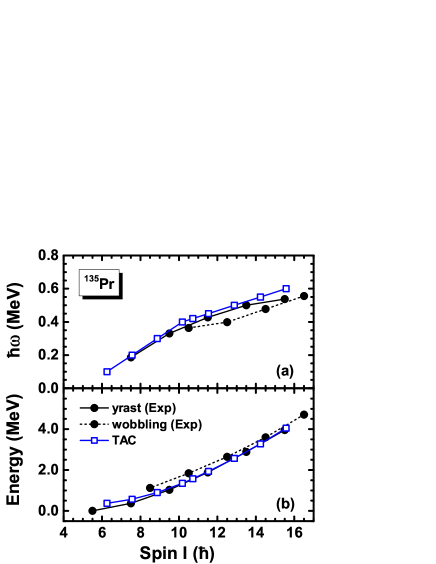
Figure 4: (Color online) Rotational frequency (upper panel) and rotational energy spectra (lower panel) of the yrast band in ${}^{135}\rm{Pr}$ as functions of the angular momentum calculated by TAC (open squares) in comparison with the data (solid dots) of Ref. Matta et al. (2015). In the TAC calculations, the quantal correction $1/2$ has been extracted for the angular momenta Frauendorf and Meng (1996).

The mass parameter in the collective Hamiltonian is calculated by the HFA approximation formula (11), where the effective MOIs induced by the proton particle are taken into account. The obtained mass parameter as well as the effective MOIs of the three principal axes are shown in Fig. 5 as functions of rotational frequency. It is seen that the MOI of axis 3, $\mathcal{J}_{3}$, remains constant, as the proton particle angular momentum has no component along the axis 3 in the HFA approximation. The effective MOI of axis 2, $\mathcal{J}_{2}^{*}$, is a constant at $\hbar\omega\leq 0.40~{}\rm{MeV}$, and increases after $\hbar\omega=0.40~{}\rm{MeV}$. The reason is that the proton particle angular momentum deviates from axis 1, moving toward axis 2 at $\hbar\omega>0.40$ MeV. The effective MOI of axis 1, $\mathcal{J}_{1}^{*}$, decreases with rotational frequency due to the factor $1/\omega$ in Eq. (9). As a consequence, the mass parameter increases with the rotational frequency as shown in Fig. 5(a). At $\hbar\omega=0.40$ MeV there is a kink, corresponding to the transition from principal axis rotation to planar rotation.

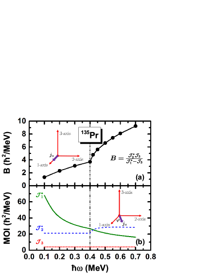
Figure 5: (Color online) The calculated mass parameter (upper panel) as well as the effective MOIs of the three principal axes $\mathcal{J}_{1}^{*}$, $\mathcal{J}_{2}^{*}$, and $\mathcal{J}_{3}$ (lower panel) as a function of rotational frequency $\hbar\omega$. A diagrammatic sketch of the angular momentum vector of the proton particle with respect to the principal axis frame is also shown.

After obtaining the collective potential and the mass parameter, the collective Hamiltonian (1) is constructed. The diagonalization of the collective Hamiltonian yields the collective energy levels and the corresponding collective wave functions. The lowest collective level at each cranking frequency corresponds to the yrast mode, and the second lowest one corresponds to the one-phonon wobbling excitation Chen et al. (2014). They are compared with the data Matta et al. (2015) in Fig. 6(a), and good agreement can be seen.

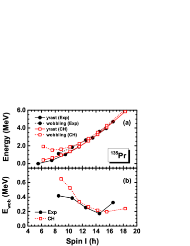
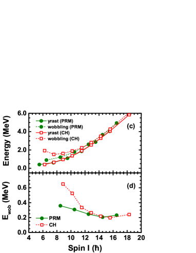
Figure 6: (Color online) Energy spectra of the yrast and wobbling bands (a) and the corresponding wobbling frequency (b) in ${}^{135}\rm{Pr}$ as functions of the angular momentum calculated by the collective Hamiltonian in comparison with the data of Ref. Matta et al. (2015). In the collective Hamiltonian results, the angular momenta are calculated from the TAC model. Similar comparisons with PRM are shown in (c) and (d).

From the energy spectra, the wobbling frequency $E_{\rm wob}$ is extracted by calculating the energy difference between the yrast and wobbling bands. The obtained $E_{\rm wob}$ as a function of spin is shown in Fig. 6(b), in comparison with the data Matta et al. (2015). At $I\leq 14.5\hbar$, both the theoretical and experimental wobbling frequencies decrease with spin, which provides the evidence of transverse wobbling motion. The theoretical calculations overestimate the data at $I<10.5\hbar$. The reason might be attributed to the fact that the HFA approximation used to derive the mass parameter is not a good approximation at low spins Chen et al. (2014). At the high spin region ($I\geq 14.5\hbar$), the experimental wobbling frequency shows an increasing trend, indicating the wobbling mode transition from transverse to longitudinal type Matta et al. (2015). The collective Hamiltonian calculations well reproduce this transition.

As mentioned in the Introduction, the PRM solutions for ¹³⁵Pr have been given in Refs. Frauendorf and Dönau (2014); Matta et al. (2015). In Figs. 6(c) and 6(d), the energy spectra and wobbling frequency obtained by the collective Hamiltonian are compared with those by the PRM. It is seen that the collective Hamiltonian can well reproduce the PRM energy spectra, except the first two states in the wobbling band. Also, for the wobbling frequency, the collective Hamiltonian has good agreement with the PRM in the high spin region ($I\geq 12.5\hbar$), but overestimates in the low spin region ($I\leq 10.5\hbar$). This implies that the approximation used in the present collective Hamiltonian in the high spin region works better than that in the low spin region.

The transition of the wobbling mode can be understood from the effective MOIs, $\mathcal{J}_{k}^{*}$. As shown in Fig. 5(b), $\mathcal{J}_{1}^{*}$ is much larger than $\mathcal{J}_{2}^{*}$ and $\mathcal{J}_{3}$ at $\hbar\omega\leq 0.40~{}\rm{MeV}$. As a result, the total angular momentum favors axis 1. This corresponds to rotation about the short axis (axis 1) and forms the transverse wobbling mode. In the large rotational frequency region, however, $\mathcal{J}_{2}^{*}$ becomes larger than $\mathcal{J}_{1}^{*}$ and $\mathcal{J}_{3}$. This leads to the tilt of the total angular momentum toward axis 2, and the transverse wobbling mode changes to the longitudinal wobbling mode.

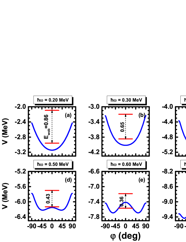
Figure 7: (Color online) Collective potential calculated by TAC model and two lowest collective energy levels obtained from the collective Hamiltonian at rotational frequencies $\hbar\omega=0.20$-$0.70~{}\rm{MeV}$. The wobbling frequency $E_{\rm wob}$ for each rotational frequency is also shown.

It is interesting to understand the variation of the wobbling frequency from the calculations of the collective Hamiltonian. In Fig. 7, the collective potentials as well as the obtained yrast and wobbling energy levels at rotational frequencies $\hbar\omega=0.20$, 0.30, 0.40, 0.50, 0.60, and $0.70~{}\rm{MeV}$ are shown. The wobbling frequency $E_{\rm wob}$ for each rotational frequency is also presented. For $\hbar\omega\leq 0.40~{}\rm{MeV}$, the collective potential is of a harmonic oscillator shape with its bottom part becoming flatter with the increase of rotational frequency. This, in combination with the increase of the mass parameter [see Fig. 5(a)], makes the wobbling excitation easier, and thus the wobbling frequency decreases, e.g., from $E_{\rm wob}=0.86$ MeV at $\hbar\omega=0.20$ MeV to $E_{\rm wob}=0.53$ MeV at $\hbar\omega=0.40$ MeV. At $\hbar\omega=0.50$ and 0.60 MeV, there appear two symmetric minima and a potential barrier between them. The continuous decrease of wobbling frequency is attributed to the appearance and increase of the barrier, which will suppress the tunneling probability between the two minima Chen et al. (2014). When $\hbar\omega\geq 0.70$ MeV, the minima of the collective potential gradually approach $\varphi=\pm 90^{\circ}$. The potential barriers at $\pm 90^{\circ}$ become much lower than that at $0^{\circ}$, and will eventually disappear at a large enough rotational frequency. As a result, the potential at $\pm 90^{\circ}$ becomes stiffer, and the wobbling excitations become harder. Thus, the wobbling frequency here shows an increasing trend.

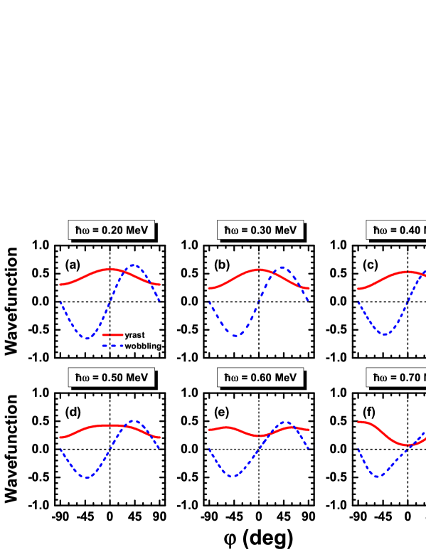
Figure 8: (Color online) Collective wave functions obtained from the collective Hamiltonian at rotational frequency $\hbar\omega=0.20$-$0.70~{}\rm{MeV}$.

The obtained wave functions of the yrast and wobbling bands at different rotational frequencies are shown in Fig. 8. It is seen that the wave functions are symmetric for the yrast band and antisymmetric for the wobbling band with respect to $\varphi\to-\varphi$ transformation. Thus the broken signature symmetry in the TAC model is restored in the collective Hamiltonian by the quantization of wobbling angle $\varphi$ and the consideration of quantum fluctuation along the $\varphi$ motion. The peak of the wave function of yrast state is located at $\varphi=0^{\circ}$ at $\hbar\omega\leq 0.40~{}\rm{MeV}$, and deviates from $\varphi=0^{\circ}$ at $\hbar\omega>0.40~{}\rm{MeV}$. This reflects the transition from the principal axis rotation to planar rotation. For the wave functions of wobbling states, which correspond to one-phonon excitations, they are odd functions and the values at $\varphi=0^{\circ}$ and $\pm 90^{\circ}$ are all zero.

V Summary and perspective

In summary, the collective Hamiltonian based on the TAC model is applied to describe the recently observed wobbling bands in ¹³⁵Pr. The collective parameters in the collective Hamiltonian, including the collective potential and the mass parameter, are calculated by the TAC model and the HFA formula, respectively.

For the yrast band, the energy spectra together with the relations between the spin and the rotational frequency can be reproduced by the TAC model with the configuration $\pi(1h_{11/2})^{1}$. Beyond the TAC mean field approximation, the collective Hamiltonian reproduces the energy spectra of both the yrast and wobbling bands well. It is confirmed that the wobbling mode in ¹³⁵Pr changes from the transverse to longitudinal one with the increase of rotational frequency. This transition is understandable by analyzing the effective MOIs of the three principal axes. It is pointed out that the effective MOI caused by the valence particle is of importance for forming different type of wobbling mode, and the softness and shapes of the collective potential determine the variation trends of the wobbling frequency.

Here, the collective Hamiltonian is constructed based on a simple single-$j$ shell model. The success of the collective Hamiltonian here guarantees its application for more realistic TAC calculations, e.g., the TAC covariant density functional theory Meng et al. (2013); Meng and Zhao (2016); Meng (2016). After such a TAC model is implemented, the collective potential and the mass parameters in the collective Hamiltonian can be obtained in a fully microscopic manner. Works along this direction are in progress.

References

- Bohr and Mottelson (1975) A. Bohr and B. R. Mottelson, Nuclear structure, Vol. II (Benjamin, New York, 1975).
- Odegaard et al. (2001) S. W. Odegaard, G. B. Hagemann, D. R. Jensen, M. Bergström, B. Herskind, G. Sletten, S. Törmänen, J. N. Wilson, P. O. Tjøm, I. Hamamoto, et al., Phys. Rev. Lett. 86, 5866 (2001).
- Frauendorf and Meng (1997) S. Frauendorf and J. Meng, Nucl. Phys. A 617, 131 (1997).
- Starosta et al. (2001) K. Starosta, T. Koike, C. J. Chiara, D. B. Fossan, D. R. LaFosse, A. A. Hecht, C. W. Beausang, M. A. Caprio, J. R. Cooper, R. Krücken, et al., Phys. Rev. Lett. 86, 971 (2001).
- Landau and Lifshitz (1960) L. D. Landau and E. M. Lifshitz, Course of Theoretical Physics: Mechanics (Pergamon, London, 1960).
- Jensen et al. (2002) D. R. Jensen, G. B. Hagemann, I. Hamamoto, S. W. Odegaard, B. Herskind, G. Sletten, J. N. Wilson, K. Spohr, H. Hübel, P. Bringel, et al., Phys. Rev. Lett. 89, 142503 (2002).
- Bringel et al. (2005) P. Bringel, G. B. Hagemann, H. Hübel, A. Al-khatib, P. Bednarczyk, A. Bürger, D. Curien, G. Gangopadhyay, B. Herskind, D. R. Jensen, et al., Eur. Phys. J. A 24, 167 (2005).
- Schönwaßer et al. (2003) G. Schönwaßer, H. Hübel, G. B. Hagemann, P. Bednarczyk, G. Benzoni, A. Bracco, P. Bringel, R. Chapman, D. Curien, J. Domscheit, et al., Phys. Lett. B 552, 9 (2003).
- Amro et al. (2003) H. Amro, W. C. Ma, G. B. Hagemann, R. M. Diamond, J. Domscheit, P. Fallon, A. Gorgen, B. Herskind, H. Hubel, D. R. Jensen, et al., Phys. Lett. B 553, 197 (2003).
- Hartley et al. (2009) D. J. Hartley, R. V. F. Janssens, L. L. Riedinger, M. A. Riley, A. Aguilar, M. P. Carpenter, C. J. Chiara, P. Chowdhury, I. G. Darby, U. Garg, et al., Phys. Rev. C 80, 041304 (2009).
- Matta et al. (2015) J. T. Matta, U. Garg, W. Li, S. Frauendorf, A. D. Ayangeakaa, D. Patel, K. W. Schlax, R. Palit, S. Saha, J. Sethi, et al., Phys. Rev. Lett. 114, 082501 (2015).
- Zhu et al. (2009) S. J. Zhu, Y. X. Luo, J. H. Hamilton, A. V. Ramayya, X. L. Che, Z. Jiang, J. K. Hwang, J. L. Wood, M. A. Stoyer, R. Donangelo, et al., Int. J. Mod. Phys. E 18, 1717 (2009).
- Luo et al. (2013) Y. X. Luo, J. H. Hamilton, A. V. Ramayya, J. K. Hwang, S. H. Liu, J. O. Rasmussen, S. Frauendorf, G. M. Ter-Akopian, A. V. Daniel, and Y. T. Oganessian, in Proceedings of the International SymposiumVladivostok, Russia, edited by Yu E. Penionzhkevich and Yu G. Sobolev (World Scientific, Singapore, 2012).
- Hartley et al. (2011) D. J. Hartley, R. V. F. Janssens, L. L. Riedinger, M. A. Riley, X. Wang, A. Aguilar, M. P. Carpenter, C. J. Chiara, P. Chowdhury, I. G. Darby, et al., Phys. Rev. C 83, 064307 (2011).
- Frauendorf and Dönau (2014) S. Frauendorf and F. Dönau, Phys. Rev. C 89, 014322 (2014).
- Hamamoto (2002) I. Hamamoto, Phys. Rev. C 65, 044305 (2002).
- Hamamoto and Mottelson (2003) I. Hamamoto and B. R. Mottelson, Phys. Rev. C 68, 034312 (2003).
- Tanabe and Sugawara-Tanabe (2006) K. Tanabe and K. Sugawara-Tanabe, Phys. Rev. C 73, 034305 (2006).
- Tanabe and Sugawara-Tanabe (2008) K. Tanabe and K. Sugawara-Tanabe, Phys. Rev. C 77, 064318 (2008).
- Sugawara-Tanabe and Tanabe (2010) K. Sugawara-Tanabe and K. Tanabe, Phys. Rev. C 82, 051303 (2010).
- Sugawara-Tanabe et al. (2014) K. Sugawara-Tanabe, K. Tanabe, and N. Yoshinaga, Prog. Theor. Exp. Phys. 2014, 063D01 (2014).
- Shi and Chen (2015) W. X. Shi and Q. B. Chen, Chin. Phys. C 39, 054105 (2015).
- Marshalek (1979) E. R. Marshalek, Nucl. Phys. A 331, 429 (1979).
- Shimizu and Matsuzaki (1995) Y. R. Shimizu and M. Matsuzaki, Nucl. Phys. A 588, 559 (1995).
- Matsuzaki et al. (2002) M. Matsuzaki, Y. R. Shimizu, and K. Matsuyanagi, Phys. Rev. C 65, 041303 (2002).
- Matsuzaki et al. (2004a) M. Matsuzaki, Y. R. Shimizu, and K. Matsuyanagi, Eur. Phys. J. A 20, 189 (2004a).
- Matsuzaki et al. (2004b) M. Matsuzaki, Y. R. Shimizu, and K. Matsuyanagi, Phys. Rev. C 69, 034325 (2004b).
- Matsuzaki and Ohtsubo (2004) M. Matsuzaki and S. I. Ohtsubo, Phys. Rev. C 69, 064317 (2004).
- Shimizu et al. (2005) Y. R. Shimizu, M. Matsuzaki, and K. Matsuyanagi, Phys. Rev. C 72, 014306 (2005).
- Shimizu et al. (2008) Y. R. Shimizu, T. Shoji, and M. Matsuzaki, Phys. Rev. C 77, 024319 (2008).
- Shoji and Shimizu (2009) T. Shoji and Y. R. Shimizu, Progr. Theor. Phys. 121, 319 (2009).
- Frauendorf and Dönau (2015) S. Frauendorf and F. Dönau, Phys. Rev. C 92, 064306 (2015).
- Chen et al. (2013) Q. B. Chen, S. Q. Zhang, P. W. Zhao, R. V. Jolos, and J. Meng, Phys. Rev. C 87, 024314 (2013).
- Chen et al. (2014) Q. B. Chen, S. Q. Zhang, P. W. Zhao, and J. Meng, Phys. Rev. C 90, 044306 (2014).
- Frauendorf and Meng (1996) S. Frauendorf and J. Meng, Z. Phys. A 356, 263 (1996).
- Meng et al. (2013) J. Meng, J. Peng, S. Q. Zhang, and P. W. Zhao, Front. Phys. 8, 55 (2013).
- Meng and Zhao (2016) J. Meng and P. W. Zhao, Phys. Scr. 91, 053008 (2016).
- Meng (2016) Relativistic density functional for nuclear structure, edited by J. Meng (World Scientific, Singapore, 2016).