ABSTRACT: A generalized attracting horseshoe is introduced as a new paradigm for describing chaotic strange attractors (of arbitrary finite rank) for smooth and piecewise smooth maps $f:Q\rightarrow Q$, where $Q$ is a homeomorph of the unit interval in $\mathbb{R}^{m}$ for any integer $m\geq 2$. The main theorems for generalized attracting horseshoes are shown to apply to Hénon and Lozi maps, thereby leading to rather simple new chaotic strange attractor existence proofs that apply to a range of parameter values that includes those of earlier proofs. In particular, it is shown that the Hénon map has a chaotic strange attractor for the popular parameter values $a=1.4$, $b=0.3$, which apparently resolves an open problem.

Keywords: Generalized attracting horseshoes, Chaotic strange attractors, Birkhoff–Moser–Smale theory, Hénon attractor, Lozi attractor

AMS Subject Classification 2010: 37D45; 37E99; 92D25; 92D40

1 Introduction

Ever since Lorenz [26] reported on what were then surprising results of the numerical simulations of his simplified, mildly nonlinear, 3-dimensional ODE model of atmospheric flows, chaotic strange attractors have been the subject of intense investigation by theoretical and applied dynamical systems researchers. Later 3-dimensional ODE models such as Rössler’s [36] analytic system and Chua’s [8] piecewise linear system further intensified the interest in these intriguing and important types of dynamical phenomena.

Over fifty years of dedicated mathematical, scientific, engineering and economic research using analytical, computational and experimental methods has firmly established that the identification and characterization of chaotic strange attractors is important for both theory and applications (see [1, 5, 7, 10, 18, 21, 22, 24, 25, 27, 30, 31, 34, 35, 37, 39, 40, 44]). However, this tends to be very difficult to achieve rigorously, especially for continuous dynamical systems, as evidenced by the fact that many properties of the Lorenz, Rössler and Chua attractors that seem clear from very precise and extensive simulations, have yet to be proven.

As discrete dynamical systems are generally easier to analyze than their continuous (ODE or PDE) counterparts, their chaotic strange attractors should be considerably easier to describe rigorously, which likely was part of the motivation for the development of an approximate Poincaré map for the Lorenz system by Hénon [19, 20]. The Hénon map is a (quadratic) polynomial diffeomorphism of the plane with iterates that converge to what appears to be a boomerang-shaped attractor, as shown in Fig.1, having the look of a fractal set with a Hausdorff dimension slightly greater than one (see [15]), and it actually rather closely resembles the simulated Poincaré map iterates of the Lorenz system for the right choice of a transversal.

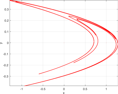
Figure 1: The Hénon attractor for $H(x,y)=(1-ax^{2}+y,bx)$ for $a=1.4$, $b=0.3$

Even though the Hénon map dynamics is considerably more amenable to analysis than the Lorenz equations, proving the existence of a chaotic strange attractor still turned out to be formidable. Possibly motivated by an interest in finding an even simpler approximation than Hénon’s, Lozi [28, 29] devised his almost everywhere analytic piecewise linear map that appeared to have a chaotic strange attractor, illustrated in Fig.2, resembling a piecewise linear analog of the one generated by $H$. But a rigorous verification of the existence of the putative chaotic strange attractor for the Lozi map proved to be quite difficult. Finally, in a pioneering investigation involving a rather lengthy proof, Misiurewicz [32] proved that the Lozi map has a chaotic strange attractor for a range of the nonnegative parameters $a$ and $b$, which to our knowledge is the first such rigorous verification for any dynamical system. The Hénon system proved to be a much tougher nut to crack, and it was not until eleven years later that Benedicks & Carleson [3] proved in an almost herculean effort involving long, detailed and subtle analysis, that the Henon map has a chaotic strange attractor for parameters near $a=2$ and $b=0$, respectively.

The fascinating record of dedicated research offers compelling evidence of the difficulty in proving the existence of strange attractors, even for relatively simple nonlinear maps. This also includes attractors that simply that display unusually high orders of complexity such as in [6, 45] and many of the books cited in our reference list, and this includes strange (fractal) attractors that are not chaotic such as in [17]. At any rate, the almost overwhelming number and diversity of chaotic strange attractors points to a real need to develop a theory or theories that subsume significant subclasses of these elusive and consequential dynamical entities; and in this progress is being made. In recent years, the basic ideas behind the proofs of the landmark Lozi and Hénon map results in strange attractor theory have been extended and generalized in terms of a theory of rank one maps in an extraordinary series of papers by Wang & Young [41, 42, 43], the content of which gives striking confirmation of the exceptional complexity underlying characterizations of strange attractors for broad classes of discrete dynamical systems. However, the foundational results of rank one theory are generally hard to prove, and they tend to be rather difficult to apply, as for example in Ott & Stenlund [34], which is closely related to results of Zaslavsky [45] and Wang & Young [42]. In light of this rather daunting rigorous chaotic strange attractor landscape, it is clear that there is a need for simpler theories and methods for reasonably ample classes of discrete dynamical systems of significant theoretical and applied interest. Our hope is that the work in this paper is a useful step in that direction.

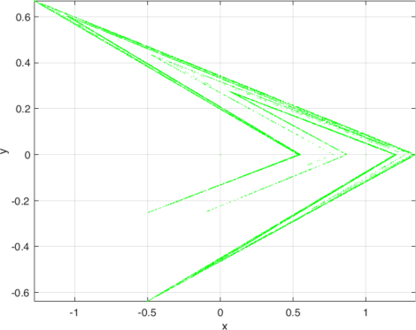
Figure 2: The Lozi attractor for $L(x,y)=(1-a\left|x\right|+y,bx)$ for $a=1.7$, $b=0.5$

The organization of the remainder of this paper is as follows. In Section 2 we describe some notation and definitions to be used throughout the exposition. This might seem unnecessary to experts, but since there are a number of competing definitions that are widely accepted, it is prudent to be very specific in certain cases. Then, in Section 3, we describe our generalized attracting horseshoe paradigm and prove the main theorem about its strange chaotic attractor. In addition, we show how related maps are subsumed by the paradigm, which leads to analogous chaotic strange attractor theorems. Moreover, we extend these results to higher dimensions, thereby obtaining rank $k$ attractors for any integer $k\geq 2$. After this, in Section 4, we apply the results in Section 3 to the Hénon and Lozi maps to obtain surprisingly short and efficient chaotic strange attractor existence theorems for each of these discrete dynamical systems. This includes analyses of natural extensions of the Hénon and Lozi maps to $\mathbb{R}^{3}$, focusing on their rank-2 attractors. The exposition concludes in Section 5 with a summary of our results and their impacts, as well as a brief description envisaged related future work.

2 Notation and Definitions

We shall be concerned here primarily with discrete (semi) dynamical systems generated by the nonnegative iterates of continuous maps

$$f:U\rightarrow\mathbb{R}^{m},$$ (1)

where $m\geq 2$, $U$ is a connected open subset of $\mathbb{R}^{m}$, $f$ is $C^{1}$ except possibly on finitely many submanifolds of positive codimension having a union that does not contain any of the fixed points of the map. Our focus shall be on planar maps ($m=2$), but we are going to consider higher dimensions in the sequel. More specifically, we are going to concentrate on maps of the form (1) having the additional property that the is a homeomorph of the unit disk $B_{1}(0):=\{\boldsymbol{x}\in$ $\mathbb{R}^{m}:\left\|\boldsymbol{x}\right\|\leq 1\}$ contained in $U$, which we denote as $Q$, such that

$$f\left(Q\right)\subset Q.$$ (2)

Employing the usual abuse of notation, we identify the restriction of $f$ to $Q$ with $f$ itself, so that our primary concern is with the dynamics of the maps

$$f:Q\rightarrow Q$$ (3)

subject to the above assumptions. We denote this set of maps as $\mathfrak{F}^{1}(Q)$ and remark that we have included the possibility of maps that may not be differentiable on sets of (Lebesgue) measure zero because we are going to analyze Lozi attractors.

Our aim is to identify and characterize attractors for maps of the form (3); in particular attractors that are fractal sets on which the restricted dynamics exhibit chaotic orbits. For our definition of chaos, we take the description ascribed to Devaney, which requires sensitive dependence on initial conditions, density of the set of periodic points and topological transitivity, keeping in mind that Banks et al. [2] proved that sensitive dependence is implied by periodic density and transitivity. For more standard definitions, we refer the reader to [1, 12, 18, 22, 25, 35, 39, 44].

We are now ready to give a precise definition of a chaotic strange attractor (CSA) - our principal object of interest.

Definition Let $f\in$$\mathfrak{F}^{1}(Q)$ and $\mathfrak{A}\subset Q$. Then $\mathfrak{A}$ is a chaotic strange attractor for $(3)$ if it satisfies the following properties:

• • it is a compact, connected,$f$-invariant subset of $Q.$

  • $\mathfrak{A}$ is an attractor in the sense that there is an open set $V$ of $\mathbb{R}^{m}$ such that $A\subset V\cap Q$ and $d\left(f^{n}(\boldsymbol{x}),\mathfrak{A}\right)\rightarrow 0$ as $n\rightarrow\infty$ for every $x\in V\cap Q$.

  • it is the minimal set satisfying CAS1 and CAS2.

3 Attracting Horseshoes and Their Generalizations

Attracting horseshoes (AH) were introduced in Joshi & Blackmore [24] as a CSA model that can be extended to any finite rank. The CSA for the AH can be readily shown to be given by

$$\mathfrak{A}:=\overline{W^{u}(p)}.$$

As one can plainly see in Fig.3, these AHs are basically the standard Smale horseshoes described in such treatments as [1, 13, 18, 25, 39, 40, 44], which were also employed by Easton [14] in his work on trellises. Attracting horseshoes have precisely three fixed points comprising two saddles points $p$ and $q$ and one sink $r$, such that $f(A)\subset B$, with $B$ contained in the basin of attraction of the sink. It should be noted that since $f(Q)$ is contained in the interior of $Q$, which is diffeomorphic to a disk in the plane, it is a simple matter to extend $f$ to a diffeomorphism $F:\mathbb{R}^{2}\rightarrow\mathbb{R}^{2}$ having $\overline{W^{u}(p)}$ as a global attractor. The main novelty in [24] was the focus on attractors, and especially multihorseshoe chaotic strange attractors produced by AHs for iterated maps, which are apt to display extraordinary complexity. Inasmuch as AHs have three fixed points - two saddles and one sink - these models are not suitable for the analysis of maps such as those of Hénon and Lozi, which have only two fixed points, both of which are saddle points. It was precisely this observation that led to our development of the generalized attracting horseshoe (GAH).

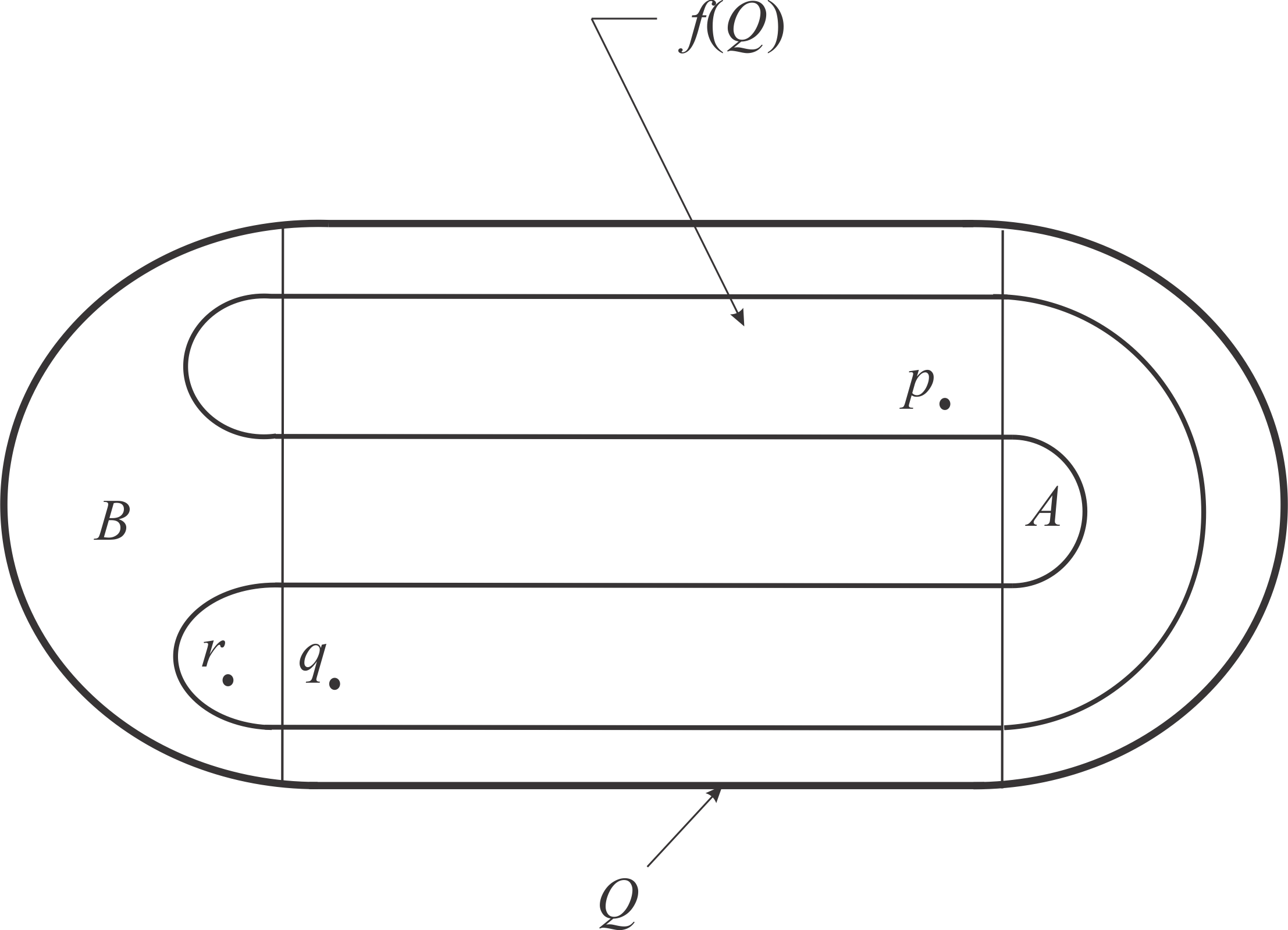
Figure 3: AH model

3.1 The generalized attracting horseshoe (GAH)

The GAH is a modification of the AH that can be represented as a geometric paradigm with either just one or two fixed points, both of which are saddles. As a result, we shall show that it includes both the Hénon and Lozi maps, which leads to simple proofs of the existence of CSAs for these maps that are essentially simple applications of the main theorems that we shall attend to in this subsection.

Figure 4 shows a rendering of a $C^{1}$ GAH with two saddle points, which can be constructed as follows: The rectangle is first contracted vertically by a factor $0<\lambda_{v}<1/2$, then expanded horizontally by a factor $1<\lambda_{h}<2$ and then folded back into the usual horseshoe shape in such a manner that the total height and width of the horseshoe do not exceed the height and width, respectively of the rectangle $Q$. Then the horseshoe is translated horizontally so that it is completely contained in $Q$. Obviously, the map $f$ defined by this construction is a member of $\mathfrak{F}^{1}(Q)$ defined in Section 2. Clearly, there are also many other ways to obtain this geometrical configuration. For example, the map $f$ as described above is orientation-preserving, and an preserving variant can be obtained by composing it with a reflection in the horizontal axis of symmetry of the rectangle, or by composing it with a reflection in the vertical axis of symmetry followed by a composition with a half-turn. Another construction method is to use the standard Smale horseshoe that starts with a rectangle, followed a horizontal composition with just the right scale factor or factors to move the image of $Q$ into $Q$, while preserving the expansion and contraction of the horseshoe along its length and width, respectively. Note that the subrectangle $S$ with its left vertical edge through $p$, which contains the arch of the horseshoe and the keystone region $K$, is to play a key role in our main theorems, which follow.

Theorem 1.

Let $f:Q\rightarrow Q$ be the member of $\mathfrak{F}^{1}(Q)$ representing the GAH paradigm with a horseshoe-like image as shown in Fig. 4. Then if $f$ satisfies the additional property

$(T)$ f maps the keystone region $K$ $($containing a portion of the arch of the horseshoe$)$ to the left of the fixed point $p$, i.e. $f(K)\subset Q\smallsetminus S=\{(x,y)\in Q:x<x(p)\}$,

$$\mathfrak{A}:=\overline{W^{u}(p)}$$

is a CSA.

Proof.

It follows from the construction that $\overline{W^{u}(p)}$ is a compact attractor, so it remains to prove that it is strange (fractal) and has chaotic orbits. But this is precisely where the property $(T)$ comes into play. For it guarantees that a strip (tubular neighborhood) around the unstable manifold of $f^{2}$ at $p$ completely crosses a strip around the stable manifold of $f^{2}$ at $p$ as shown in Fig. 5, which presents a magnified picture of the image $f^{2}\left(Q\right)$ in a neighborhood of $p$. Hence, we conclude from the well-known results of Birkhoff–Moser–Smale (cf. [33, 40, 44]), and a slight generalization for the crossing of stable and unstable manifolds is not necessarily transverse (see, eg. [24]), that the attractor locally has the structure of the Cartesian product of a Cantor middle-third set and an interval, and exhibits (symbolic) shift map chaotic dynamics. ∎

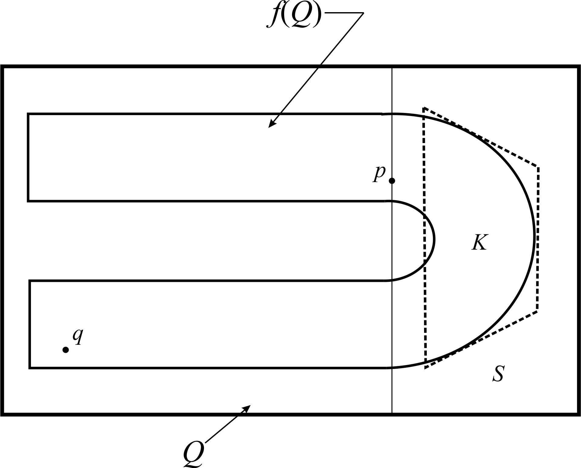
Figure 4: A planar GAH with two saddle points

Theorem 1 can readily be adapted to cover even more general horseshoe-like maps in $\mathfrak{F}^{1}(Q)$, with virtually the same proof.

Theorem 2.

Let $f:Q\rightarrow Q$ be any member of $\mathfrak{F}^{1}(Q)$ with a horseshoe-like image with a keystone region $K$ containing a portion of the arch of $f(Q)$ analogous to that shown in Fig.4. Suppose that the map is expanding by a scale factor uniformly greater than one along the length of the horseshoe and contracting transverse to it by a scale factor uniformly less than one-half in the complement of a subset of Q containing K. Then if $f$ satisfies the additional property

$(\tilde{T})$ f maps K into an open subset of Q to the left of the saddle point p,

$$\mathfrak{A}:=\overline{W^{u}(p)}$$

is a CSA.

Proof.

This follows mutatis mutandis from the proof of Theorem 1. ∎

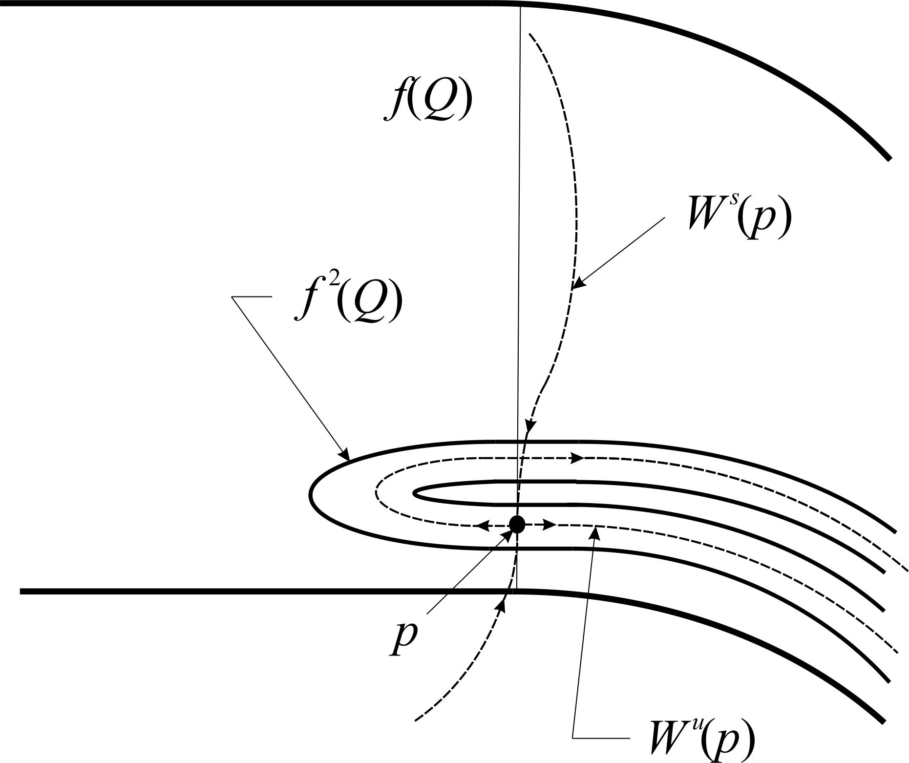
Figure 5: Local (transverse) horseshoe structure of $f^{2}$ near $p$

3.2 Higher dimensional GAH paradigms

The planar GAH model can be extended to any finite dimension to produce CSAs of any rank. For example, this can be accomplished inductively by composing the paradigm with the model map in successive coordinate planes formed by the contracting coordinate and each new (expanding) coordinate direction that is added. For demonstration purposes, it suffices to show how to go from a 1-dimensional unstable manifold to a 2-dimensional unstable manifold in $\mathbb{R}^{3}$.

We may write the planar GAH in the form

$$f(x,y):=\left(u(x,y),v(x,y)\right),$$ (4)

which we extend to Euclidian 3-space as

$$f_{1}(x,y,z):=\left(f(x,y),z\right)=\left(u(x,y),v(x,y),z\right).$$ (5)

Then, holding $x$ fixed and applying the planar model map in the $z$-$y$ coordinate plane corresponds to the mapping

$$f_{2}(x,y,z):=\left(x,v(z,y),u(z,y)\right).$$ (6)

Therefore, the desired extension is

$$f_{3}(x,y,z):=f_{2}\circ f_{1}(x,y,z)=f_{2}\left(u(x,y),v(x,y),z\right)=\left(u(x,y),v\left(z,v(x,y)\right),u\left(z,v(x,y)\right)\right).$$ (7)

Higher dimensional GAH paradigms and, more generally, GAH models of the type covered in Theorem 2 of any finite dimension can be created by successive applications of the inductive step described above, which allows to construct GAHs of any rank. To visualize the nature of the image of $f_{3}$, picture a thickened plane perpendicular to the $z$-axis that is first folded quite sharply along the $x$-axis and then folded rather more gently along the $z$-axis.

4 Applications to the Hénon and Lozi Maps

The existence of CSAs for the Hénon and Lozi maps now turn out to be direct corollaries of Theorem 2. We consider the Hénon map

$$H(x,y):=\left(1-ax^{2}+y,bx\right)$$ (8)

for a small parameter neighborhood of $(a,b)=(1.4,0.3)$ and the Lozi map

$$L(x,y):=\left(1-\alpha\left|x\right|+y,\beta x\right)$$ (9)

in a parameter neighborhood of $(\alpha,\beta)=(1.7,0.5)$ that their (apparent) respective CSAs at $(a,b)=(1.4,0.3)$ and $(\alpha,\beta)=(1.7,0.5)$ are illustrated in Fig. 1 and Fig. 2, respectively.

Our first result is for the Hénon map (8), which has a quadrilateral trapping region $Q$, first observed in [20], with vertices at $A$: (-1.33,0.42), $B$: (1.32,0.133), $C$: (1.245,-0.14) and $D$: (-1.06,-0.5). The map has just two fixed points, $p$ and $q$, both of which are saddles. The fixed points are (approximately):

$$p=(0.631354477,0.189406)\ \text{and}\ q=(-1.131354477,-0.339406343),$$

and we note that only $p\in Q$.

Theorem 3.

The Hénon map $(\ref{eq8})$ has a CSA given by

$$\mathfrak{A}:=\overline{W^{u}(p)}$$

in a sufficiently small parameter neighborhood of $(a,b)=(1.4,0.3)$.

Proof.

It is straightforward to prove that the trapping quadrilateral $Q$, with vertices $A$, $B$, $C$ and $D$ given above, is such that (8) is a member of $\mathfrak{F}^{1}(Q)$ and it satisfies the hypotheses of Theorem 2 for a sufficiently small neighborhood of $(a,b)=(1.4,0.3)$. We shall now verify this, leaving some of the routine details to the reader. To begin, we show that the map satisfies property $(\tilde{T})$, which entails proving that a properly chosen keystone set is mapped to the left of the fixed point $p$. First we find the extremes of the intersection of $H(Q)$ with the $x$-axis. Owing to the nature of the map, this can be done by computing the images of the endpoints of the vertical line corresponding to $x=0$ in $Q$. It is convenient to denote the upper and lower endpoints by $a_{+}$ and $a_{-}$, respectively. The endpoint $a_{+}$ is the intersection point of the $y$-axis and the edge $AB=(1-t)A+tB$ $(0\leq t\leq 1)$, which we compute by solving the following equations for $t_{+}$ and then $y:=y(a_{+})$:

$$(1-t_{+})(-1.33)+t_{+}(1.32) =0\Longrightarrow t_{+}=\frac{1.33}{2.65},\;(1-t_{+})(0.42)+t_{+}(0.133)=$$

$$0.42-0.287t_{+} =\frac{0.73129}{2.65}=y\approx 0.276\Longrightarrow a_{+}\approx(0,0.276).$$

Similarly, $a_{-}$ is the point of intersection of the $y$-axis and the edge $DC=(1-t)D+tC$ $(0\leq t\leq 1)$, which we determine by solving

$$(1-t_{-})(-1.06)+t_{-}(1.245) =0\Longrightarrow t_{-}=\frac{1.06}{2.305},\;(1-t_{-})(-0.5)+t_{-}(-0.14)=$$

$$-0.5+0.36t_{-} =-\frac{0.7709}{2.305}=y(a_{-})\approx-0.3344\Longrightarrow a_{-}\approx(0,-0.3344).$$

Whence, we compute that $H(a_{+})\approx(1.276,0)$ and $H(a_{-})\approx(0.6655,0)$, and more precisely that the intersection of $H(Q)$ with the $x$-axis, comprising the ‘centerline’ of the arch of the horseshoe, is a closed interval contained in $(0.6655,1.276)\times\{0\}$. Consequently, we may choose the keystone $K$ so that it is completely contained in the subset $Q_{K}$ of $Q$ consisting of points $(x,y)$ with $x\geq x_{K}:=0.65$. It is easy to see that from (8) and the definition of the trapping quadrilateral $Q$, that in order to show that $H(Q_{K})$ lies to the left of the saddle point $p$, it suffices to show that he intersection point of the vertical line $x=x_{K}$ with the edge $AB$, which we denote by $z$, is mapped to the left of $p$ by $H$. To compute $z$, we solve the equations

$$(1-t_{z})(-1.33)+t_{z}(1.32) =0.65\Longrightarrow t_{z}=\frac{1.98}{2.65},\;(1-t_{z})(0.42)+t_{z}(0.133)=$$

$$0.42-0.287t_{z} =\frac{0.54474}{2.65}=y(z)\approx 0.2056\Longrightarrow z\approx(0.65,0.2056).$$

Hence, $H(z)\approx\left(1-1.4(0.65)^{2}+0.2056,0.3(0.65)\right)=(0.6141,0.195)$. More precisely, the $x$-coordinate of $H(z)$ is strictly less than $0.62<0.63<x(p)$, which verifies property $(\tilde{T}).$ Next, we shall show that $H$ is expanding along the length of the horseshoe by focusing on the foliation of $Q$ along its width by the family of line segments for $0\leq s\leq 1$ defined as

$$l_{s}:=\left(-1.33+0.27s+2.65t-0.345st,0.42-0.92s-0.287t+0.647st\right)\;(0\leq t\leq 1).$$

Note that $l_{0}$ and $l_{1}$ correspond to the edges $AB$ and $DC$, respectively. Moreover, as the left and right endpoints of $l_{s}$ are, respectively, $(-1.33+0.27s,0.42-0.92s)$ and $(1.32-0.075s,0.133-0.273s)$, it follows that the length of $l_{s}$ is

$$\mathcal{L}\left(l_{s}\right)=\left(7.104869-2.199878s+0.537634s^{2}\right)^{1/2},$$

which is a strictly decreasing function of $s$ for $0\leq s\leq 1$ such that $2.3<\mathcal{L}\left(l_{s}\right)<2.7$. The images $H\left(l_{s}\right)$ are parabolas that foliate $H(Q)$, and we shall prove the expansiveness along the length by showing that

$$\mathcal{L}H\left(l_{s}\right)>3.2$$

for all $s\in[0,1]$. The Euclidean equation of each of the lines can be readily shown to have the form

$$l_{s}:y=\alpha(s)+m(s)x,$$

where the slope is

$$m(s):=\frac{0.647s-0.287}{2.65-0.345s}$$

and

$$\alpha(s):=0.42+0.92s+m(s)(1.33-0.27s).$$

It is useful to note that

$$\left|m(s)\right|<0.1562$$

and $\alpha$ is a strictly decreasing function of $s$ satisfying

$$0.275<\alpha(s)<1.51$$

for all $0\leq s\leq 1$. Whence, it is straightforward to show using

$$\xi=1-1.4x^{2}+y,\;\eta=0.3x,$$

that the image $H\left(l_{s}\right)$ has, for each $s\in[0,1]$, the following representation in the $\xi,\eta$-plane:

$$\xi-\left(1+\alpha(s)+\frac{35m^{2}}{196}\right)=-\frac{140}{9}\left(\eta-\frac{3m}{28}\right)^{2},$$

which is a parabola with axis of symmetry $\eta=3m/28$ - a horizontal line within a distance of $0.017$ of the $\xi$-axis for all $0\leq s\leq 1.$ Furthermore, since it is easy to show that

$$H\left(AD\right),H\left(BC\right)\subset Q_{(-1)}:=\{(x,y)\in Q:x<-1\},$$

which implies that each of the above parabolic arcs have endpoints in $Q_{(-1)}$. Moreover, all of the parabolas lie between the extremes

$$H\left(l_{0}\right):\xi-1.278052=-\frac{140}{9}\left(\eta+0.011604\right)^{2}$$

and

$$H\left(l_{1}\right):\xi-0.669909018=-\frac{140}{9}\left(\eta-0.016733808\right)^{2}$$

so their maximal $\xi$ values are all greater than $0.6.$ Hence, the positions of their endpoints implies that $\mathcal{L}H\left(l_{s}\right)>3.2$ for all $s\in[0,1]$, which proves that the map is expanding along the horseshoe. One nice feature of the geometric argument above is that it can also be used to verify the necessary transverse contraction property. Indeed, it is easy to show that $H$ is contracting by a factor of absolute value less than $0.5$ along the vertical in $\xi,\eta$-plane in the complement of the ‘keystone’ set described in the first part of our proof. Thus, the existence of the CSA for the map (8) with $(a,b)=(1.4,0.3)$ of the specified type is guaranteed by Theorem 2. Finally, noting that all of the elements used in the above argument, including the vertices of the trapping set, the position and type of the fixed points and the vertices of the keystone set are all continuous functions of the parameters in a sufficiently small neighborhood of $(a,b)=(1.4,0.3)$, we obtain the desired result and the proof is complete. ∎

We note here that the above result appears to solve an open problem concerning the existence of a chaotic strange attractor for the specified parameter values. Regarding the fractal nature of the CSA, numerical simulation methods have been used in [38] to show that the Hausdorff dimension of the Hénon attractor for $(a,b)=(1.4,0.3)$ is approximately equal to $1.26$.

The existence proof for the Lozi map (9) also follows with ease. It can be readily shown to have a triangular trapping region $Q$ with vertices at $A$: (-1.28392467,0.671742549), $B$: (1.3434851,0) and $C$: (-0.51092939,-0.641962335), and just two fixed points, both saddles; namely,

$$p=(0.4545454,0.2272727)\ \text{and}\ q=(-0.8333333,-0.4166666),$$

with only $p\in Q$.

Theorem 4.

The Lozi map $(\ref{eq9})$ has a CSA given by

$$\mathfrak{A}:=\overline{W^{u}(p)}$$

in a sufficiently small parameter neighborhood of $(\alpha,\beta)=(1.7,0.5)$.

Proof.

It can readily be proved that (9) is for the triangle (a degenerate quadrilateral) $Q$, with vertices $A$, $B$, and $C$ defined above, a member of $\mathfrak{F}^{1}(Q)$ (failing to be differentiable only along the $y$-axis) that satisfies the hypotheses of Theorem 2 for a sufficiently small neighborhood of $(\alpha,\beta)=(1.7,0.5)$. We show this, omitting some routine detail,s in a manner analogous that used to prove Theorem 3. We begin by showing that the map satisfies property $(\tilde{T})$, which requires demonstrating that a properly chosen keystone set is mapped to the left of the fixed point $p$. The first step is to compute the extremes of the intersection of $L(Q)$ with the $x$-axis. It follows from the definition of the map $L$ that this can be done by computing the images of the endpoints of the vertical line corresponding to $x=0$ in $Q$. As in the proof of Theorem 3, we denote the upper and lower endpoints by $a_{+}$ and $a_{-}$, respectively. Since the endpoint $a_{+}$ is the intersection point of the $y$-axis and the edge $AB=(1-t)A+tB$ $(0\leq t\leq 1)$, we need to solve the following equations for $t_{+}$ and then $y:=y(a_{+})$:

$$(1-t_{+})(-1.28392467)+t_{+}(1.3434581) =0\Longrightarrow t_{+}=\frac{1.28392467}{2.62740977},\;(1-t_{+})(0.671742549)+t_{+}(0)=$$

$$\frac{0.902405167}{2.62740977} =y\approx 0.3434581\Longrightarrow a_{+}\approx(0,1.3434581).$$

Analogously, $a_{-}$ is the point of intersection of the $y$-axis and the edge $CB=(1-t)C+tB$ $(0\leq t\leq 1)$, which can be determined by solving

$$(1-t_{-})(-0.51092939)+t_{-}(1.3434851) =0\Longrightarrow t_{-}=\frac{0.51092939}{1.85441449},\;(1-t_{-})(-0.641962335)+t_{-}(0)=$$

$$-\frac{0.862466831}{1.85441449} =y(a_{-})\approx-0.46509\Longrightarrow a_{-}\approx(0,-0.46509).$$

Consequently, we compute that $L(a_{+})\approx(1.34349,0)$ and $L(a_{-})\approx(0.53491,0)$, and a closer examination of the computations shows that the intersection of $L(Q)$ with the $x$-axis, comprising the ‘centerline’ of the pointed arch of the horseshoe, is a closed interval contained in $(0.53491,1.34349)\times\{0\}$. Accordingly we may choose the keystone $K$ so that it is completely contained in the subset $Q_{K}$ of $Q$ consisting of points $(x,y)$ with $x\geq x_{K}:=0.5$. It is readily deduced from (9) and the definition of the trapping triangle $Q$, that in order to show that $L(Q_{K})$ lies to the left of the saddle point $p$, it suffices to show that he intersection point of the vertical line $x=x_{K}$ with the edge $AB$, which we denote by $z$, is mapped to the left of $p$ by $L$. The value of $z$ can be obtained by solving the following equations:

$$(1-t_{z})(-1.28392467)+t_{z}(1.3434851) =0.5\Longrightarrow t_{z}=\frac{1.78392467}{2.62740977},\;(1-t_{z})(0.671742549)+t_{z}(0)=$$

$$\frac{0.566604831}{2.62740977} =y(z)\approx 0.2157\Longrightarrow z\approx(0.5,0.2157).$$

Hence, $L(z)\approx\left(1-1.7\left|0.5\right|+0.2157,0.5(0.5)\right)=(0.3657,0.195)$. And a more careful examination of the calculations shows that the $x$-coordinate of $L(z)$ is strictly less than $0.37<0.45<x(p)$, which proves that property $(\tilde{T})$ is satisfied. We shall next verify that $L$ is expanding along the length of the horseshoe and that it is contracting in a transverse direction. Rather than taking a geometric approach analogous to that used in the proof of Theorem 3, we shall use a method that takes advantage of the fact that the derivative of $L$, where it exists, is piecewise constant. Note that, in terms of the standard matrix representation, we have

$$L^{\prime}(x,y)=\left\{\begin{array}[c]{cc}\mathcal{D}_{-},&x<0\\ \mathcal{D}_{+},&x>0\end{array}\right.,$$

where

$$\mathfrak{D}_{-}:=\left(\begin{array}[c]{cc}1.7&1\\ 0.5&0\end{array}\right)\text{ and }\mathfrak{D}_{+}:=\left(\begin{array}[c]{cc}-1.7&1\\ 0.5&0\end{array}\right).$$

Consequently, the scale factor of the map $L$ along any direction specified by the unit vector $\boldsymbol{\hat{u}}(\theta):=(\cos\theta,\sin\theta)$ is given either by

$$\sigma_{-}(\theta):=\left|\left\langle\mathfrak{D}_{-}\boldsymbol{\hat{u}}(\theta),\boldsymbol{\hat{u}}(\theta)\right\rangle\right|=1.7\cos^{2}\theta+0.75\sin 2\theta\text{ or }\sigma_{-}(\theta):=\left|\left\langle\mathfrak{D}_{-}\boldsymbol{\hat{u}}(\theta),\boldsymbol{\hat{u}}(\theta)\right\rangle\right|=-1.7\cos^{2}\theta+0.75\sin 2\theta.$$

To verify the expanding nature of the map along the horseshoe, we consider the (singular) foliation of $Q$ by the rays emanating for $B$ that are contained in the triangle between the two extremes, $AB$ and $CB$, with the slopes linearly increasing from the upper to the lower edge. The corresponding range of angles (in degrees) is from

$$\tan\theta_{AB}=\frac{\Delta y}{\Delta x}=\frac{-0.671742549}{2.62740977}\approx-0.255667219\Longrightarrow\theta_{AB}\approx-14.34144088^{o}$$

to

$$\tan\theta_{CB}=\frac{\Delta y}{\Delta x}=\frac{0.641962335}{1.85441449}\approx 0.346180607\Longrightarrow\theta_{CB}\approx 19.09486124^{o}.$$

Whence, we find for the interval $\left[-14.34144088^{o},19.09486124^{o}\right]$ that

$$\min\sigma_{-}(\theta)\geq 1.231\text{ and }\min\sigma_{-}(\theta)\geq 1.054.$$

As both of these minima exceed one, and we can ignore the behavior along $x=0$ owing to the fact that it has Lebesgue measure zero, the map is expanding along the horseshoe. It remains to prove that the map is contracting transverse to the horseshoe. The vertical direction should be avoided because $L$ maps small vertical line segments to the left and right of the $y$-axis into horizontal line segments. However, any near vertical (singular) foliation can be used. In this regards, a simple calculation along the lines of those above shows that

$$\max\sigma_{-}(\theta),\max\sigma_{-}(\theta)\leq 1/2$$

whenever $75^{o}\leq\theta\leq 105^{0}$, which verifies the transverse contraction of the map $L.$ Thus, it follows from Theorem 2 that the theorem is proved for $(\alpha,\beta)=(1.7,0.5)$. Therefore, owing to the local continuous dependence on of all the key features used in the proof such as the position and type of the fixed point $p$ and the vertices of the trapping triangle $Q$, the desired result follows, which completes the proof. ∎

The above theorems provide a great deal of information about the long-term dynamics of the Hénon and Lozi maps, which when combined with Cvitanović’s pruning techniques and kneading theory such as in [10, 11, 23] ought to reveal a great deal about the nature of the iterates of the mappings. In this regard, see also [13]. We note that it appears that the above theorems for the Hénon and Lozi maps can also be proved using rank one theory, possibly with minor modifications. However, the rather obvious extensions to higher dimensional maps of these results, which can be proved using an analogous combination of geometric and analytic tools,  are not directly amenable to rank one theory verification.

4.1 Higher dimensional Hénon and Lozi maps

Three-dimensional extensions of the Hénon and Lozi maps can be easily obtained by the inductive process developed in Section 3. In particular, the extensions to $\mathbb{R}^{3}$ are

$$H_{3}(x,y,z):=\left(1-ax^{2}+y,\bar{b}z,1-az^{2}+bx\right),$$ (10)

and

$$L_{3}(x,y,z):=\left(1-\alpha\left|x\right|+y,\bar{\beta}z,1-\alpha\left|z\right|+\beta x\right),$$ (11)

where typically we have to choose $0<b/a,\bar{b}/a$ and $0<\beta/\alpha,\bar{\beta}/\alpha$ considerably smaller than the corresponding ratio in Theorem 3 and Theorem 4, respectively, to compensate for the lack of symmetry in the trapping regions, which would be unnecessary for the GAH paradigm shown in Fig. 4. We note that it is interesting to compare (11) with the results in [16]. Examples of attractors for three-dimensional Hénon and Lozi maps are shown in Fig.6 and Fig.7, respectively. These attractors in $\mathbb{R}^{3}$ are automatically CSAs, and one can infer from the figures that each has a Hausdorff dimension somewhat greater than two.

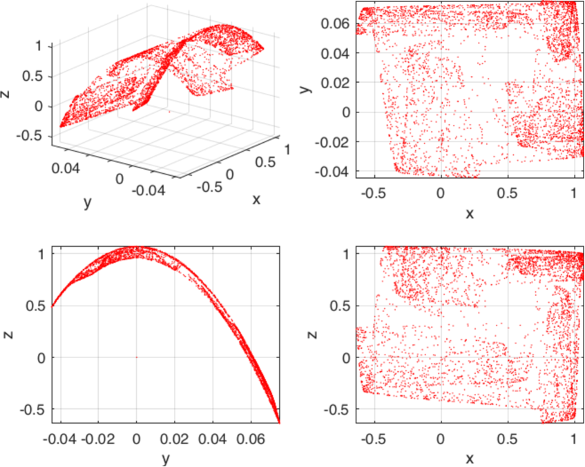
Figure 6: Local Attractor for the map (10) for $a=1.4$, $b=\bar{b}=0.09$. Clockwise: full 3D; projections in $x,y$; $x,z$ and $y,z$ planes.

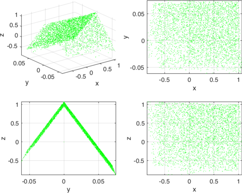
Figure 7: Local Attractor for the map (11) for $\alpha=1.7$, $\beta=\bar{\beta}=0.08$. Clockwise: full 3D; projections in $x,y$; $x,z$ and $y,z$ planes.

5 Concluding Remarks

We have introduced GAH dynamical models proved that they have CSAs that are closures of unstable manifolds of any finite dimension. Moreover, by showing that they include the Hénon and Lozi maps of the plane, we were able to give comparatively simple proofs that they possess CSAs for certain parameter values, and in the process resolved an apparently open question of rather long standing about the existence of a CSA for the Hénon map with parameters $a=1.4$ and $b=0.3$. The models presented are those having 1-dimensional stable manifolds for their key saddle points, so it is natural to also consider models having higher dimensional stable manifolds for these points, which we plan to do in the near future. In addition, along the lines in [4, 9], we intend to construct SRB measures for the GAH paradigms, thereby enabling a deeper statistical study of their CSAs. Finally, we have observed that our CSA constructions appear to have some important applications in granular flow problems, and we intend to seek out additional areas of science and engineering in which GAHs may be useful.

References

- [1] D. K. Arrowsmith and C. M. Place, Dynamical Systems: Differential Equations, Maps and Chaotic Behaviour, Chapman and Hall, London, 1992.
- [2] J. Banks, J. Brooks, G. Cairns, G. Davis and P. Stacey, On Devaney’s definition of chaos, Amer. Math. Monthly 99 (1992), 332-334.
- [3] M. Benedicks and L. Carleson, The dynamics of the Hénon map, Ann. of Math. (2) 133 (1991), 73-169.
- [4] M. Benedicks and L.-S. Young, SBR measures for certain Hénon maps, Invent. Math. 112 (1993), 541-576.
- [5] D. Blackmore, A. Rosato, X. Tricoche, K. Urban and L. Zuo, Analysis, simulation and visualization of 1D tapping dynamics via reduced dynamical models, Physica D 273-274 (2014), 14-27.
- [6] H. Bruin, G. Keller, T. Nowicki and S. van Strien, Wild Cantor attractors exist, Ann. of Math. 143 (1996), 97-130.
- [7] L. Chen and K. Aihara, Strange attractors in chaotic neural networks, IEEE Trans. Circ. Syst. 47 (2000), 1455-1468.
- [8] L. Chua, M. Komuro and T. Matsumoto, The double scroll family, IEEE Trans. Circuits and Systems 33 (1986), 1072-1118.
- [9] P. Collet and Y. Levy, Ergodic properties of the Lozi mappings, Comm. Math. Phys. 93 (1984), 461-481. (SRB measure for Lozi)
- [10] P. Cvitanović, 1991 Periodic orbits as the skeleton of classical and quantum chaos, Physica D 51 (1991), 138-151.
- [11] P. Cvitanović, G. Gunaratne G and I. Procaccia, Topological and metric properties of Hénon-type strange attractors, Phys. Rev. A 38 (1991) 1503-1520.
- [12] R. Devaney, An Introduction to Chaotic Dynamics, Addison-Wesley, Boston, 1989.
- [13] R. Devaney and Z. Nitecki, Shift automorphisms in the Hénon mapping, Comm. Math. Phys. 67 (1979), 137-146.
- [14] R. Easton, Trellises formed by stable and unstable manifolds in the plane, Trans. Amer. Math. Soc. 294 (1986), 719-732.
- [15] K. Falconer, Techniques in Fractal Geometry, Wiley, Chichester, U.K., 1997.
- [16] S. Gonchenko, J. Meiss and I. Ovsyannikov, Chaotic dynamics of three-dimensional Hénon maps that originate from a homoclinic bifurcation, Regular Chaotic Dyn. 11, 191-212.
- [17] C. Grebogi, E. Ott, S. Pelikan and J. Yorke, Strange attractors that are not chaotic, Physica D 13 (1984), 261-268.
- [18] J. Guckenheimer and P. Holmes, Nonlinear Oscillations, Dynamical Systems and Bifurcations of Vector Fields, Springer-Verlag, New York, 1983.
- [19] M. Hénon, Numerical study of quadratic area preserving mappings, Q. Appl. Math. 27 (1969), 291-312.
- [20] M. Hénon, A two-dimensional mapping with a strange attractor, Comm. Math. Phys. 50 (1976), 69-77.
- [21] P. Holmes and F. Moon, Strange attractors and chaos in nonlinear mechanics, J. Appl. Mech. 50 (1983), 1021-1032.
- [22] B. Hunt, J. Kennedy, T.-Y. Li and H. Nusse (eds), The Theory of Chaotic Attractors, Springer-Verlag, New York, 2004.
- [23] Y. Ishii, Towards a kneading theory for Lozi mappings, II: A solution of the pruning front conjecture and the first tangency problem, Nonlinearity 10 (1997), 731-747.
- [24] Y. Joshi and D. Blackmore, D., Strange attractors for asymptotically zero maps, Chaos, Solitons & Fractals 68 (2014), 123-138.
- [25] A. Katok and B. Hasselblatt, Introduction to the Modern Theory of Dynamical Systems, Cambridge University Press, Cambridge, 1995.
- [26] E. Lorenz, Deterministic nonperiodic flow, J. Atmosph. Sci. 20 (1963), 130 - 141.
- [27] H. Lorenz, Strange attractors in a multisector business cycle model, J. Econ. Behavior & Organization 8 (1987), 397-411.
- [28] R. Lozi, Un attracteur étrange (?) du type attracteur de Hénon, Journal de Physique 39 (1978), C5–9.
- [29] R. Lozi, Strange attractors: a class of mappings of R2 which leaves some Cantor sets invariant, Intrinsic Stochasticity in Plasmas (Internat. Workshop, Inst. Études Sci. Cargeşe, Cargeşe, 1979) (Palaiseau: ÉcolePolytech) pp. 373–81.
- [30] J. Milnor, On the concept of attractor, Comm. Math. Phys. 99 (1985), 177-195.
- [31] J. Milnor, Correction and remarks: “On the concept of attractor”, Comm. Math. Phys. 102 (1985), 517-519.
- [32] M. Misiurewicz, Strange attractors for the Lozi mappings, N.Y. Acad. Sci. 357 (1980), 348-358.
- [33] J. Moser, Stable and Random Motions in Dynamical Systems, Princeton University Press, 2001.
- [34] W. Ott and M. Stenlund, From limit cycles to strange attactors, Comm. Math. Phys. 296 (2010), 215-249.
- [35] C. Robinson, Dynamical Systems: Stability, Symbolic Dynamics, and Chaos, CRC Press Inc., Boca Raton, 1995.
- [36] O. Rössler, An equation for continuous chaos, Phys. Lett. A 57 (1976), 397-398.
- [37] D. Ruelle, Chaotic Evolution and Strange Attractors, Lezioni Lincee, Cambridge Univ. Press, Cambridge, 1989.
- [38] D. Russell, J. Hanson and E. Ott, Dimension of strange attractors, Phys. Rev. Lett. 45 (1980), 1175-1178.
- [39] M. Shub, Global Stability of Dynamical Systems, Springer-Verlag, New York, 1987.
- [40] S. Smale, The Mathematics of Time, Springer-Verlag, New York, 1980.
- [41] Q. Wang and L.-S. Young, Strange attractors with one dimension of instability, Comm. Math. Phys. 218 (2001), 1-97.
- [42] Q. Wang and L.-S. Young, From invariant curves to strange attractors, Comm. Math. Phys. 225 (2002), 275-304.
- [43] Q. Wang and L.-S. Young, Toward a theory of rank one attractors, Ann. of Math. (2) 167 (2008), 349-480.
- [44] S. Wiggins, Introduction to Applied Nonlinear Dynamical Systems and Chaos, Springer, New York, 2003.
- [45] G. Zaslavsky, The simplest case of a strange attractor, Phys. Lett. A 69 (1978/79), 145-147.