Meson masses and decay constants at large $N$

Abstract:

Meson masses and decay constants in the large $N$ limit of SU($N$) gauge theory are determined using the twisted Eguchi-Kawai reduced model. To this end, we make use of a recently defined smearing method valid on the one-point lattice. This procedure, in combination with a variational analysis, allows to obtain reliable values for these quantities.

1 Introduction

The Twisted Eguchi-Kawai model (TEK-model) is a $SU(N)$ lattice gauge theory having only one site with twisted boundary conditions [1, 2]. It has been shown that this model is equivalent to the usual lattice gauge theory in the large $N$ limit [3, 4]. In fact, we have succeeded in calculating the large $N$ string tension and running coupling constant in the continuum limit starting from the TEK model [5, 6]. We have also shown that it is straightforward to introduce adjoint fermions within our framework [7, 8]. Last year, two of us proposed a new method to calculate meson correlators in this set up  [9, 10]. This problem was actually quite challenging for two main reasons:

• Quarks in the fundamental representation are not consistent with the twist.

• Meson propagators are space-time extended objects not easily defined within the one-site lattice model.

Both caveats can be solved by allowing quarks to propagate in a bigger lattice than the one seen by the periodic (up to the twist) gauge fields. This has allowed to compute the large $N$ ground state meson spectrum, using for simplicity point-point meson correlators [9, 10]. However, it was not possible to reliably estimate decay constants due to the contamination from excited states. The purpose of the present talk is to make use of the smearing method introduced in [10], which combined with a variational analysis makes it possible to calculate both meson masses and decay constants.

2 Formulation

In this section we will briefly review the construction of the meson correlators in the TEK model, further details can be consulted in refs. [9, 10]. We formulate the $SU(N)$ gauge theory, with $N=L^{2}$, on a 4-dimensional one-point lattice with twisted boundary conditions given by the antisymmetric twist tensor: $n_{\nu\mu}=kL$, for $\mu>\nu$. The integers $L$ and $k$ should be coprime and obey certain constraints to prevent center symmetry breaking [3]. In the large $N$ limit, this theory is equivalent to the usual $SU(N)$ lattice gauge theory defined on a $L^{4}$ lattice.

We will consider that quark fields live on a finite box $\ell_{0}L\times L^{3}$, with positive integer $\ell_{0}$. In ref. [9], we have shown that the correlation function at time separation $n_{0}$ of two local, zero-momentum meson operators in channels $\gamma_{A}$ and $\gamma_{B}$ is given by:

$$C_{AB}(n_{0})={1\over\ell_{0}N^{3/2}}\sum_{q_{0}}{\rm e}^{-iq_{0}n_{0}}{\rm Tr}\left[\gamma_{A}D^{-1}(0)\gamma_{B}D^{-1}(q_{0})\right],$$ (1)

with momentum $q_{0}$ quantized in units of $\ell_{0}L$. The Wilson-Dirac operator acts on colour ($U_{\mu}$), spatial ($\Gamma_{\mu}$), and Dirac ($\gamma_{\mu}$) indexes, and is given by:

$$D(q_{0})=1-\kappa\sum_{\mu=0}^{d-1}\left[(1-\gamma_{\mu}){\tilde{U}_{\mu}}\Gamma_{\mu}^{*}+(1+\gamma_{\mu}){\tilde{U}_{\mu}^{\dagger}}\Gamma_{\mu}^{t}\right],$$ (2)

with ${\tilde{U}_{\mu}}=\exp(iq_{\mu}\delta_{\mu,0})\,U_{\mu}$, and with $\Gamma_{\mu}$ the $SU(N)$ matrices satisfying

$$\Gamma_{\mu}\Gamma_{\nu}=\exp(2\pi in_{\nu\mu}/N)\Gamma_{\nu}\Gamma_{\mu}.$$ (3)

An explicit form for these matrices, usually called twist eaters, is shown, for example, in eq.(2.13) of ref. [4].

Although one can compute meson masses from these local correlators, the effective mass plots show a clear contamination from excited states [10]. To obtain improved results, we have proposed to use the smearing method originally introduced in [11] adapted to the one-point lattice [10]. Smearing can be easily implemented by replacing $\gamma_{A}$ in eq. (1) by the operator:

$$\gamma_{A}\rightarrow D_{s}^{l}\gamma_{A},\ \ \ D_{s}\equiv{1\over 1+6c}\left[1+c\sum_{i=1}^{d-1}\left({\bar{U}_{i}}\Gamma_{i}^{*}+{\bar{U}_{i}^{\dagger}}\Gamma_{i}^{t}\right)\right].$$ (4)

Here, $l$ is the smearing level and ${\bar{U}_{i}}$ is the APE-smeared spatial link variable obtained after iterating several times the following transformation

$$U^{\prime}_{i}={\rm Proj_{SU(N)}}\left[(1-f)U_{i}+{f\over 4}\sum_{j\neq i}(U_{j}U_{i}U_{j}^{\dagger}+U_{j}^{\dagger}U_{i}U_{j})\right]\ ,$$ (5)

with $c$ and $f$ free smearing parameters.

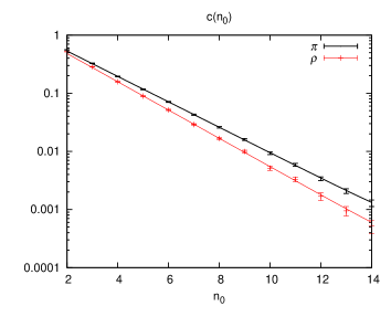
Figure 1: $SS$ correlators for $\pi$ and $\rho$.

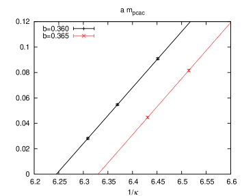
Figure 2: $1/\kappa$ dependence of $am_{\rm PCAC}$.

To improve the ground state signal we have used in addition a variational method. We start by selecting a basis of operators in each quantum channel. This is done for fixed APE-smearing of the gauge fields by changing the smearing level $l$ of the fermionic operator. We have selected ten smearing steps $\ell=$ 0, 1, 2, 3, 4, 5, 10, 20, 50, 100, and computed the $10\times 10$ correlation matrices $C_{AB}(n_{0})$ with matrix components:

$$C_{AB}^{ll^{\prime}}(n_{0})={1\over\ell_{0}N^{3/2}}\sum_{q_{0}}{\rm e}^{-iq_{0}n_{0}}{\rm Tr}\left[D_{s}^{l}\gamma_{A}D^{-1}(0)D_{s}^{l^{\prime}}\gamma_{B}D^{-1}(q_{0})\right].$$ (6)

We then solve the generalized eigenvalue problem (no summation over $A$ implied):

$$C_{AA}(n_{0}=t_{2})v_{A}=\lambda_{A}C_{AA}(n_{0}=t_{1})v_{A},$$ (7)

with $t_{1}=1$ and $t_{2}=2$. After this, we select the eigenvector corresponding to the largest eigenvalue in each channel, denoted by $v_{A}^{1}$. Smeared-smeared and local-smeared correlators are then constructed for arbitrary $n_{0}$ as

$$C_{AB}^{SS}(n_{0}) = \sum_{\ell,\ell^{\prime}}\ \ (v_{A}^{1})^{*}_{\ell}\ \ C_{AB}^{\ell\ell^{\prime}}(n_{0})\ (v_{B}^{1})_{\ell^{\prime}},$$ (8)

$$C_{AB}^{LS}(n_{0}) = \sum_{\ell^{\prime}}\ \ C_{AB}^{0\ell^{\prime}}(n_{0})\ (v_{B}^{1})_{\ell^{\prime}}.$$ (9)

In the following, $SS$ correlators will be used to determine meson masses, while $LS$ correlators will allow for the determination of decay constants in a way to be described below.

We show in fig. 2 the $SS$ pion and rho correlators for $N=289$ and $l_{0}=2$, at $b=0.36$ and $\kappa=0.155$, from which a precise determination of the masses can be obtained. For this plot, the smearing parameters have been set to $c=0.4$, $f=0.15$ and we performed 10 Ape-iterations of the gauge fields. We are currently working on a systematic analysis of the effects associated to the choice of operators in the correlation matrix. In the range of $\kappa$ and $\beta$ values of our simulations a basis of 8 to 10 smearing operators seems to be optimal for reducing the excited state contamination without loosing precission in the effective masses. A next step involves solving the generalized eigenvalue problem at all values of $t_{2}$ in eq. (7), as discussed in [12].

3 Simulations and results

To test our method, we have simulated the TEK model for $N$=289, with $\ell_{0}=2$. We took two values of inverse ’t Hooft coupling ($b=1/g_{0}^{2}N$) and two or three values of $\kappa$,

$$b = 0.360,\ \ \ \kappa=0.1555,0.157,0.1585,$$ (10)

$$b = 0.365,\ \ \ \kappa=0.1535,0.1555.$$ (11)

For each parameter set, we have calculated meson propagators with 800 configurations, each configuration being separated by 1000 MC sweeps [13]. In the following, all meson masses are obtained from a single hyperbolic cosine fit to the $SS$ correlator in each channel, with the fitting range $6\leq n_{0}\leq 12$.

The first quantity we study is the PCAC-quark mass. Following ref. [11], we compute it from a constant fit to:

$$am_{\rm PCAC}(n_{0})={C^{LS}_{\gamma_{0}\gamma_{5},\gamma_{5}}(n_{0}+1)-C^{LS}_{\gamma_{0}\gamma_{5},\gamma_{5}}(n_{0}-1)\over 4C^{LS}_{\gamma_{5},\gamma_{5}}(n_{0})}.$$ (12)

In fig. 2, we show the $1/\kappa$ dependence of $am_{\rm PCAC}$. In the case were we have three values of $\kappa$ a linear fit provides a very good fit to the data. Fig. 4 displays $(m_{\pi}/\sqrt{\sigma})^{2}$ as a function of $m_{\rm PCAC}/\sqrt{\sigma}$. The value of string tension is extracted from ref. [5], and is given by $a^{2}\sigma=0.04234(103)$ and $a^{2}\sigma=0.03181(60)$ for $b=0.36$ and $b=0.365$ respectively. The straight line is a linear fit to the data at $b$=0.360 setting the pion residual mass to zero. It is important to note that in the large $N$ limit, there should be no quenched chiral log [14, 15]. Therefore the verification of the linear dependence of $(m_{\pi}/\sqrt{\sigma})^{2}$ on $m_{\rm PCAC}/\sqrt{\sigma}$ is a non-trivial consistency check that we are really studying the dynamics of large $N$ QCD.

In fig. 4, we show the dependence of $m_{\rho}/\sqrt{\sigma}$ on $m_{\rm PCAC}/\sqrt{\sigma}$. Again, the straight line is a linear fit of the data at $b$=0.360. The results at $b$ =0.36 and 0.365 exhibit a very good scaling behavior. The horizontal line in fig. 4 is the value of $m_{\rho}/\sqrt{\sigma}$ given in [11] which is obtained by extrapolating $m_{\rho}$ at finite $N$ to $N\to\infty$, and comes out very consistent with our determination. Scaling violations seem to be really small, taking into account that no continuum extrapolation has been performed in either case.

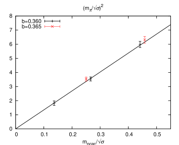
Figure 3: $m_{\rm PCAC}/\sqrt{\sigma}$ dependence of $(m_{\pi}/\sqrt{\sigma})^{2}$.

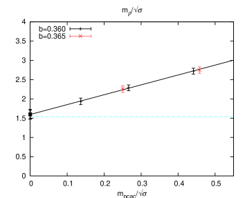
Figure 4: $m_{\rm PCAC}/\sqrt{\sigma}$ dependence of $m_{\rho}/\sqrt{\sigma}$.

Finally, we calculate the pion decay constant $f_{\pi}^{\rm lat}$. For that we first compute the correlator between the local axial-vector operator and the smeared pion operator:

$$C^{LS}_{\gamma_{0}\gamma_{5},\gamma_{5}}(n_{0})=C_{A_{0}}{\rm e}^{-n_{0}m_{\pi}}.$$ (13)

This decays exponentially in time with the pion mass. The coefficient $C_{A_{0}}$ is related to the decay constant through:

$$C_{A_{0}}=f_{\pi}^{\rm lat}\sqrt{{N\over 3}m_{\pi}C_{\pi}}$$ (14)

where $C_{\pi}$ can be extracted from the $SS$ pion correlator:

$$C^{SS}_{\gamma_{5},\gamma_{5}}(n_{0})=C_{\pi}{\rm e}^{-n_{0}m_{\pi}}.$$ (15)

We fit simultaneously these two correlators to hyperbolic sine and cosine functions respectively in the fitting range $6\leq n_{0}\leq 12$, keeping as free parameters: $m_{\pi}$, $C_{\pi}$ and $f_{\pi}$. An example of the quality of our fits is shown on fig. 6, for the same set of configurations as in fig. 2. The results for the pion mass come out compatible with the previous determination based only on the $SS$ correlator.

This gives the unrenormalized pion decay constant. To connect with the continuum decay constant, we follow [11] and use the one-loop improved $Z_{A}$ renormalization factor [16]

$$Z_{A}=1-0.4694{\lambda_{E}\over 4\pi},\ \ \ \lambda_{E}=-8{\rm ln}U_{P},$$ (16)

$$Z_{A}(b=0.36)=0.8256,\ \ \ Z_{A}(b=0.365)=0.8314.$$ (17)

The final result for the pion decay constant as a function of the PCAC quark mass is displayed in fig. 6. Both quantities are given in units of the square root of the string tension. The results show a very good scaling behaviour and nicely extrapolate in the chiral limit to the result obtained by standard large $N$ techniques in [11], indicated by the blue horizontal line in the plot.

4 Conclusions

We have shown that our smearing method, when combined with a variational analysis, works quite well and allows to determine the pion and rho masses, as well as the pion decay constant for the TEK model. Our results are consistent with those obtained using standard large $N$ techniques as in [11].

In the future we plan to extend our results making full use of the generalized eigenvalue method to give a precise estimate of the masses and decay constants in the continuum limit. These results will include the evaluation of other channels such as scalar, tensor and axial-vector. Other interesting extensions are possible and included in the future plans. The study of large $N$ 2-dimensional QCD seems an interesting testing ground, since the meson mass spectra is known in that case as the solution of an integral equation in the continuum limit [17]. Preliminary results are presented in these proceedings [18]. An interesting case is that of $SU(N)$ field theories with adjoint fermions with varying number of flavors, which has received much attention in connection with possible extensions of the Standard Model. The configurations needed for the determination of the meson spectrum are already available as a by-product of our computation of the mass anomalous dimension for these theories [7, 8].

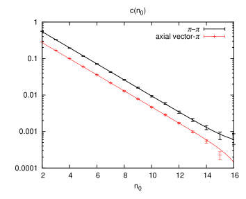
Figure 5: $\gamma_{5}$-$\gamma_{5}$, and $\gamma_{0}\gamma_{5}$-$\gamma_{5}$ correlators.

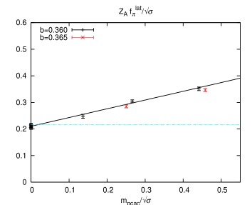
Figure 6: $m_{\rm PCAC}/\sqrt{\sigma}$ dependence of $Z_{A}f_{\pi}^{\rm lat}/\sqrt{\sigma}$.

- [1] A. Gonzalez-Arroyo and M. Okawa, Phys. Lett. B 120 (1983) 174.
- [2] A. Gonzalez-Arroyo and M. Okawa, Phys. Rev. D 27 (1983) 2397.
- [3] A. Gonzalez-Arroyo and M. Okawa, JHEP 07 (2010) 043 [arXiv:1005.1981 [hep-th]].
- [4] A. Gonzalez-Arroyo and M. Okawa, JHEP 12 (2014) 106 [arXiv:1410.6405 [hep-lat]].
- [5] A. Gonzalez-Arroyo and M. Okawa, Phys. Lett. B 718 (2013) 1524 [arXiv:1206.0049 [hep-th]].
- [6] M. Garcia Perez, A. Gonzalez-Arroyo, L. Keegan and M. Okawa, JHEP 01 (2015) 038 [arXiv:1412.0941 [hep-lat]].
- [7] A. Gonzalez-Arroyo and M. Okawa, Phys. Rev. D 88 (2013) 014514 [arXiv:1305.6253 [hep-lat]].
- [8] M. Garcia Perez, A. Gonzalez-Arroyo, L. Keegan and M. Okawa, JHEP 08 (2015) 034 [arXiv:1506.06536 [hep-lat]].
- [9] A. Gonzalez-Arroyo and M. Okawa, Phys.Lett. B 755 (2016) 132 [arXiv:1510.05428 [hep-lat]].
- [10] A. Gonzalez-Arroyo and M. Okawa, PoS LATTICE2015 (2016) 291 [arXiv:1511.00477 [hep-lat]].
- [11] G. Bali, F. Bursa, L. Castagnini, S. Collins, L. Del Debbio, B. Lucini and M. Panero, JHEP 06 (2013) 071 [arXiv:1304.4437 [hep-lat]].
- [12] B. Blossier, M. Della Morte, G. von Hippel, T. Mendes and R. Sommer, JHEP 04 (2009) 094 [arXiv:0902.1265 [hep-lat]].
- [13] M. Garcia Perez, A. Gonzalez-Arroyo, L. Keegan, M. Okawa and A. Ramos, JHEP 06 (2015) 093 [arXiv:1505.05784 [hep-lat]].
- [14] C. W. Bernard and M. Golterman, Phys. Rev. D 46 (1992) 853 [arXiv:hep-lat/9204007].
- [15] S. R. Sharpe, Phys. Rev. D 46 (1992) 3146 [arXiv:hep-lat/9205020].
- [16] A. Skouroupathis and H. Panagopoulos, Phys. Rev. D 76 (2007) 094514 Erratum: [Phys. Rev. D 78 (2008) 119901] [arXiv:0707.2906 [hep-lat]].
- [17] G. ’t Hooft, Nucl. Phys. B 75 (1974) 461.
- [18] M. Garcia Perez, A. Gonzalez-Arroyo, L. Keegan and M. Okawa, PoS LATTICE2016 (2016) 337.