Extended and localized Hopf-Turing mixed-mode in non-instantaneous Kerr cavities

Abstract

We investigate the spatio-temporal dynamics of a ring cavity filled with a non-instantaneous Kerr medium and driven by a coherent injected beam. We show the existence of a stable mixed-mode solution that can be either extended or localized in space. The mixed-mode solutions are obtained in a regime where Turing instability (often called modulational instability) interacts with self-pulsing phenomenon (Andronov-Hopf bifurcation). We numerically describe the transition from stationary inhomogeneous solutions to a branch of mixed-mode solutions. We characterize this transition by constructing the bifurcation diagram associated with these solutions. Finally, we show stable localized mixed-mode solutions, which consist of time-periodic oscillations that are localized in space.

I Introduction

Transition from spatially uniform state to a self-organized or ordered structures is a universal feature in far from equilibrium systems and has been observed in many natural systems (see overviews on this issue Rev12 ; Rev13 ; Leblond-Mihalache ; Tlidi-PTRA ; Tlidi_Clerc_sringer ). This transition is triggered by a few number of modes often called Turing modes that leads to the formation of spatially stationary structures that can be either periodic or localized in space. On the order hand, a transition to a time oscillation or a self-pulsing state through the Andronov-Hopf (termed Hopf in the following) bifurcation has also been observed. These transitions are responsible for the symmetry breaking in space (Turing) and in time (Hopf). The interaction between Turing and Hopf bifurcations concerns almost all fields of nonlinear science such as biology, chemistry, physics, fluid mechanics, and optics. When both instabilities are close one to another, the space-time dynamics of various spatially extended systems may be significantly impacted. In particular, it has been shown that in this regime either a bistable behavior between Turing patterns and self-pulsing states or front waves between Hopf and Turing-type domains may occur Bistab_HOpf_TURING2 ; Bistab_HOpf_TURING3 ; Bistab_HOpf_TURING4 ; Bistab_HOpf_TURING5 ; Barcella ; Martine_JOPB_2004 . Moreover, mixed-mode solutions resulting from the interplay between Andronov-Hopf and Turing modes may dominate the spatio-temporal dynamics in optical frequency conversion systems Tlidi_haelterman97 ; Tlidi_haelterman98 . This interaction can also lead to a spatio-temporal chaos Dewel2 .

In this paper, we consider a ring cavity filled with a non instantaneous and a nonlocal Kerr medium, and driven by a coherent injected beam. We show that the threshold associated with Turing and Hopf bifurcations can occur arbitrarily close one to another leading to codimension-two point where both bifurcations coincide. In the monostable regime, we show that the Turing pattern becomes unstable and leads to the formation of a Turing-Hopf mixed-mode. More importantly, we show that localized mixed-mode solutions can be stabilized when the system exhibits a coexistence between an homogeneous steady state and an extended mixed-mode solution.

II Model equations and a linear stability analysis

The slowly varying envelope of the electric field $E=E(x,t)$ circulating inside the cavity is described by $\partial E/\partial z=inE+i\partial^{2}E/\partial x^{2}$ coupled with an additional equation for the material photoexcitation $n=n(x,t)$: $\gamma^{-1}\partial n/\partial z=|E|^{2}+d\partial^{2}n/\partial x^{2}$ with $z$ is the longitudinal coordinate, and the parameter $d$ is proportional to the ratio between the diffusion length and diffraction coefficients. This parameter describes the degree of nonlocality. Indeed, if $d=0$, the above propagation equations have a local nonlinear response. The strong nonlocal response is characterized by a large $d$. The parameter $\gamma$ is proportional to the ratio between the characteristics decay times associated with the electric field and the refractive index $n$, respectively. At each round trip, the light inside the Kerr media is coherently superimposed with the input beam. This can be described by the cavity boundary conditions $E(z=0,x)=rS+\tau E(L,x)\exp{(i\phi_{e})}$ and $E(z=0,x)=rn(L,x)\exp{(i\phi_{n})}$, with $\phi_{e,n}$ are linear phase shifts, $S$ is the ampliude of the injected field, and $L$ denotes the cavity length. The letters ”$r$” and ”$\tau$” indicate the transmission and the reflexion coefficients. We adopt the well know mean field approach proposed by Lugiato and Lefever LL . A detailled calculations of the derivation of the mean field model can be found in the appendix of the paper Kockaert_2006 . This approach is valid under the following approximations: the cavity possesses a high Fresnel number and we assume that the cavity length is much shorter than the diffraction, diffusion and the nonlinearity spatial scales. A single longitudinal mode operation is also assumed. The mean field approach applied to our system leads to the adimensional coupled partial differential equations

$$\frac{\partial E}{\partial t} = S-(1+i\delta)E+inE+i\frac{\partial^{2}E}{\partial x^{2}},$$ (1)

$$\gamma\frac{\partial n}{\partial t} = -n+|E|^{2}+d\frac{\partial^{2}n}{\partial x^{2}},$$ (2)

where $\delta$ is the frequency detuning between the injected light and the cavity resonance. $S$ is the injected field amplitude considered as being real without loss of generality. Diffraction of the electric field in the transverse $x$ coordinate is modeled by $i\partial^{2}E/\partial x^{2}$. The density of material photoexcitation is denoted by $n$ that diffuses according to $\partial^{2}n/\partial x^{2}$. In the limit of $\delta=0$, the model has been derived for a Kerr medium but in a single feedback mirror configuration Firth90 . For a ring cavities, and in the particular limit where $d=0$ and $\gamma=0$, one obtains from Eq. (2) $n=|E|^{2}$. By replacing $n$ by $|E|^{2}$ in Eqs. (1), we recover the well known Lugiato-Lefever (LL) equation LL . The model Eqs. (1) and 2) may be viewed as an extension of LL equation to include the non instantaneous response of the medium and the nonlocal effects.

Homogeneous steady state (HSS) solutions of Eqs. (1) and (2) are found by setting the time and space derivatives equal to zero: $n_{s}=I_{s}$ and $S^{2}=I_{s}[1+(\delta-I_{s})^{2}]$ with $I_{s}=|E_{s}|^{2}$. The characteristic $I_{s}$ as a function of the input intensity $S^{2}$ is monstable when $\delta<\sqrt{3}$. The HSS’s undergo a bistable behavior when $\delta>\sqrt{3}$. The linear stability analysis of the HSS with respect to a finite wavelength perturbation of the form $\exp{(\lambda t+ikx)}$ leads to the third-order polynomial characteristic equation: $a_{0}+a_{1}\lambda+a_{2}\lambda^{2}+a_{3}\lambda^{3}=0$, with $a_{0}=1-I_{s}^{2}+(I_{s}-Q)^{2}+dk^{2}(1+Q^{2})$, $a_{1}=2(1+dk^{2})+\gamma(1+Q^{2})$, $a_{2}=1+2\gamma+dk^{2}$ and $a_{3}=\gamma$, with $Q=\delta-I_{s}+k^{2}$. The Turing type of bifurcation occurs when $\lambda=0$ and $\partial\lambda/\partial k^{2}=0$. The threshold associated with this instability and the critical wavelength at the Turing bifurcation are obtained from the expression $a_{0}=0$. This instability is characterized by an intrinsic wavelength which is determined by the dynamical parameters and not by the external geometrical constraints such as boundary conditions.

A Hopf bifurcation occurs if a pair of complex-conjugate roots has a vanishing real part and a nonzero imaginary part. In the limit $\gamma=1$ and $\delta<2$, only one Hopf bifurcation point is possible. The associated critical intensity is explicitly given by $I_{H}=2(2-\delta d)(d+\sqrt{d^{2}+1})$. At this bifurcation point the real part vanishes at nonzero wavenumber $k_{H}^{2}=-\delta+(2-\delta d)/\sqrt{d^{2}+1}$. Note that the HSS’s may undergo a homogeneous Hopf bifurcation where the real part of the eigenvalues vanishes for $k=0$.

We are interested in the regime where Turing and Hopf instabilities are close one to another. For this purpose, we fix $\gamma=1$ and $\delta=1$, and we vary the coefficient $d$ and the input field intensity. An important and interesting feature is that the parameter $d$ controls the relative position of the thresholds associated with both Turing and Hopf instabilities. Typical marginal stability curves are shown in Fig. 1. By increasing the value of the parameter $d$, the first bifurcation is of Turing type, and the Hopf bifurcation appears as secondary instability as shown in Fig. 1(a). There exists a critical value of the parameter $d$ for which both bifurcations coincide, i.e., $I_{H}=I_{T}=I_{c}$ as shown in Fig. 1(b). At this co-dimensional two point, one of the real roots of the characteristic equation vanishes $\lambda=0$ with a non zero finite intrinsic wave length $2\pi/k_{c}$ and two other roots are purely imaginary $\lambda=\pm i\omega$. Note that the critical mode $k_{c}$ is also$d$-dependent. When further increasing $d$, the first instability is the Hopf bifurcation followed by the Turing instability as shown in Fig. 1(c).

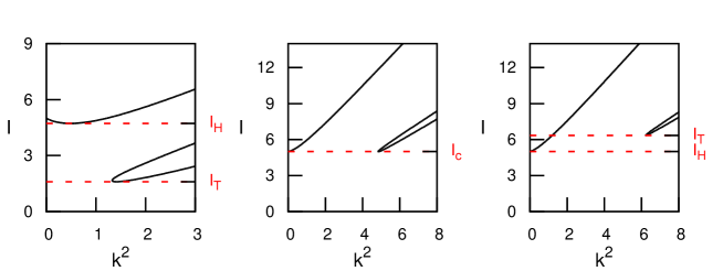
Figure 1: Marginal stability curves. The parameters are $\gamma=1$, $\delta=1$ with $I_{H}$ and $I_{T}$ are Hopf and Turing instability thresholds, respectively. (a) $d=0.4$, above the upper curve HSS is Hopf unstable. Inside the lower curve, HSS is Turing unstable. (b) $d=0.81$, note the co-dimension two instability where Turing and Hopf thresholds coincide. (c) $d=0.85$, the situation is inverted with respect to (a).

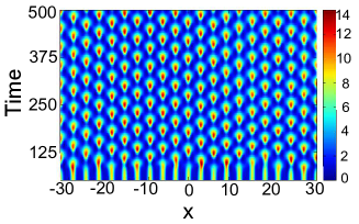
Figure 2: Space-time map showing the formation of a Turing-Hopf mixed-mode solution. The parameters are $\gamma=1$, $\delta=1$, $S=5.28$ and $d=0.4$.

Figure 3: Bifurcation diagram showing the evolution of the intracavity field intensity as a function of the input field amplitude. Stable (unstable) homogeneous steady states are indicated by solid (dotted) line. Filled squares denote the maximum intensity of the stationary periodic structures. Empty squares indicate the maximum intensity associated with mixed-mode solutions. Parameters are $\gamma=1$, $\delta=1$, and $d=0.4$.

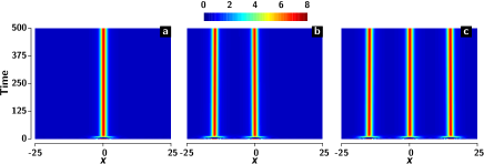
Figure 4: Space-time maps displaying the formation of multi-peaks stationary localized structures. (a) one, (b) two and (c) three peaks obtained by numerical simulations of Eqs. (1) and (2) for the parameters $\gamma=1.3$, $\delta=3$, $S=1.9$, and $d=1.45$.

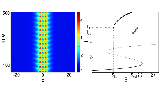
Figure 5: (a) Space-time map showing the generation of a localized mixed-mode solution. Parameters are $\gamma=1.3$, $\delta=3$, $S=2.11$, and $d=1.45$. (b) Bifurcation diagram showing the evolution of the intracavity field intensity as a function of the input field amplitude. Stable (unstable) homogeneous steady states are indicated by solid (dotted) line. Filled squares denote the maximum intensity of the stationary localized structures. Empty squares indicate the maximum intensity associated with localized mixed-mode solutions. Same parameters as in (a) with varying $S$.

III Extended and localized mixed-mode

In what follows we focus on numerical investigations of the model Eqs. (1) and (2) by using an adaptive step-size Bulirsch-Stoer method Hairer_1993 . We choose parameters values such that the homogeneous steady state is destabilized first by Turing instability. From this bifurcation point, a branch of stationary spatially periodic solutions appears supercitically with a well defined wavelength. However, when increasing further the injected field intensity a stable mixed-mode solution is spontaneously generated in the system. These solutions correspond to oscillations both in time and in space. A typical example of such a behavior is plotted in Fig. 2. To characterize the transition from stationary periodic patterns to a branch of mixed-mode Turing-Hopf structures, we plot in Fig. 3 the maxima of both Turing structures and mixed-mode solutions together with the homogeneous steady state. As we increase the amplitude of the injected field, the HSS becomes unstable, and a spatially periodic structure emerges from the Turing bifurcation point $S=S_{T}$. These structures are stable in the parameter range $S_{T}<S<S_{MM}$. For $S>S_{MM}$, the Turing structure becomes unstable and bifurcates to a stable mixed-mode solution.

The extended solutions either Turing structures or mixed-mode solutions are obtained in the supercritical regime. Besides these extended structures there exists another type of solutions which are aperiodic but localized in space (LS’s). The latter are found in the subcritical regime associated with the Turing instability. It is well known that the emergence of these solutions does not necessarily requires a bistable regime Tlidi_94 . The prerequisite condition for the generation of LS’s is the coexistence between a single HSS and the spatially periodic solutions. This solutions have been predicted theoretically Scorggie_csf94 and experimentally evidenced in an instantaneous and local optical Kerr medium Majid_NJP . Notice that temporal localized solutions known also as temporal solitons have also been experimentally observed in a dispersive Kerr cavity in Leo . Here we show that in the case of a non-instantaneous and a nonlocal Kerr medium, modeled by the Eqs. (1) and (2), support localized structures. An example of such a behavior is shown in Fig. 4. We show in this figure only localized structures with one, two and three peaks. The number of localized peaks and their spatial distributions are determined by the initial conditions Scorggie_csf94 . There exists an infinite number of spatially localized solutions if the size of the system is infinite. When increasing the injected field intensity, localized structures exhibit a pulsing phenomenon, i.e., time oscillations in a wide range of parameters leading to the formation of Hopf-Turing mixed-mode solutions. A typical example of such a behavior is shown in Fig. 5(a). The maxima of intensity associated with localized structures and localized mixed-mode solutions are plotted together with the homogeneous steady states in Fig. 5(b). When increasing the input intensity, a single peak stationary localized structure is formed in the range $S_{SL}<S<S_{MM}$. For $S>S_{MM}$, stable localized mixed-mode solutions are generated. Their maximum intensity are shown in Fig. 5(b). The width of these time dependent structures varies in the course of time.

IV Conclusions

We have shown that extended mixed-mode solutions can be generated in the output of a driven ring cavity filled with a non-instantaneous and a nonlocal Kerr medium. Our investigations are focused on the regime where Turing and Hopf instabilities interact strongly. In the monostable regime, the mixed-mode solutions appear as a transition from spatially periodic structures. We have drawn the bifurcation diagram showing their stability domain. In the bistable regime, we have shown occurrence of stationary localized structures that exhibit multistability in a finite range of parameters. Finally, we have established evidence of localized mixed-mode solutions that emerge from the branch of a single peak localized structures. We have constructed a bifurcation diagram associated with these localized structures.

References

- (1) M. Tlidi, M. Taki, and T. Kolokolnikov, ”Introduction: dissipative localized structures in extended systems,” Chaos, 17, 037101 (2007).
- (2) N. Akhmediev and A. Ankiewicz (eds.), Dissipative Solitons: from Optics to Biology and Medicine (Lecture Notes in Physics, volume 751, 2008).
- (3) H. Leblond and D. Mihalache, ”Models of few optical cycle solitons beyond the slowly varying envelope approximatio,” Phy. Rep. 523, 61 (2013).
- (4) M. Tlidi, K. Staliunas, K. Panajotov, A.G. Vladimiorv, and M. Clerc, ”Localized structures in dissipative media: from optics to plant ecology,” Phil. Trans. R. Soc. A 372, 20140101 (2014).
- (5) M. Tlidi and M.G. Clerc (eds.), Nonlinear Dynamics: Materials, Theory and Experiments (Springer Proceedings in Physics, 173, 2016).
- (6) H. Kidachi, ”On mode interactions in reaction diffusion equation with nearly degenerate bifurcations,” Prog. Theor. Phys. 63, 1152 (1980).
- (7) A.B. Rovinsky and M. Menzinger, ”Interaction of Turing and Hopf bifurcations in chemical systems,” Phys. Rev. A 46, 6315 (1992).
- (8) J.-J. Perraud, A. De Wit, E. Dulos, P. De Kepper, G. Dewel, and P. Borckmans, ”One-dimensional spirals: Novel asynchronous chemical wave sources,” Phys. Rev. Lett. 71, 1272 (1993).
- (9) G. Heidemann, M. Bode, and H.-G. Purwins, ”Fronts between Hopf- and Turing-type domains in a two-component reaction-diffusion system,” Phys. Lett. A 177, 225 (1993).
- (10) A. Barsella, C. Lepers, M. Taki, and M. Tlidi, ”Moving localized structures in quadratic media with a saturable absorber,” Opt. commun. 232, 381 (2004).
- (11) M. Tlidi, M. Taki, M. Le Berre, E. Reyssayre, A. Tallet, and L. Di Menza, ”Moving localized structures and spatial patterns in quadratic media with a saturable absorber,” J. Opt. B: Quantum and Semiclassical Optics 6, S421 (2004).
- (12) M. Tlidi and M. Haelterman, ”Robust Hopf-Turing mixed-mode in optical frequency conversion systems,” Phy. Lett. A 239, 59 (1998).
- (13) M. Tlidi, P. Mandel, and M. Haelterman, ”Spatiotemporal patterns and localized structures in nonlinear optics,” Phys. Rev. E 56, 6524 (1997).
- (14) A. De Wit, D. Lima, G. Dewel, and P. Borckmans, ”Spatiotemporal dynamics near a codimension-two point,” Phys. Rev. E 54, 261 (1996).
- (15) W.J. Firth, ”Spatial instabilities in a Kerr medium with single feedback mirror,” J. Mod. Opt. 37, 151 (1990).
- (16) L. A. Lugiato and R. Lefever, ”Spatial dissipative structures in passive optical systems,” Phys. Rev. Lett. 58, 2209 (1987).
- (17) P. Kockaert, P. Tassin, G. Van der Sande, I. Veretennicoff, and M. Tlidi, ”Negative diffraction pattern dynamics in nonlinear cavities with left-handed materials,” Phy. Rev. A 48, 4605 (2006).
- (18) E. Hairer, S.P. NÞrsett, and G. Wanner, Solving ordinary differential equations I: Nonstiff problem (Springer-Verlag, 1993).
- (19) M. Tlidi, P. Mandel, and R. Lefever, ”Localized structures and localized patterns in optical bistability,” Phys. Rev. Lett. 73, 640 (1994).
- (20) A.J. Scorggie, W.J. Firth, G.S. McDonald, M. Tlidi, R. Lefever, and L.A. Lugiato, ”Pattern formation in a passive Kerr cavity,” Chaos, Solitons & Fractals, 4, 1323 (1994).
- (21) V. Odent, M. Taki, and E. Louvergneaux, ”Experimental evidence of dissipative spatial solitons in an optical passive Kerr cavity,” New J. Phys. 13, 113026 (2011).
- (22) F. Léo, L. Gelens, Ph. Emplit, M. Haelterman, and S. Coen, ”Dynamics of one-dimensional Kerr cavity solitons,” Opt. Express 21, 9180 (2013).