Cosmological model from the holographic equipartition law
with a modified Rényi entropy

Abstract

Cosmological equations were recently derived by Padmanabhan from the expansion of cosmic space due to the difference between the degrees of freedom on the surface and in the bulk in a region of space. In this study, a modified Rényi entropy is applied to Padmanabhan’s ‘holographic equipartition law’, by regarding the Bekenstein–Hawking entropy as a nonextensive Tsallis entropy and using a logarithmic formula of the original Rényi entropy. Consequently, the acceleration equation including an extra driving term (such as a time-varying cosmological term) can be derived in a homogeneous, isotropic, and spatially flat universe. When a specific condition is mathematically satisfied, the extra driving term is found to be constant-like as if it is a cosmological constant. Interestingly, the order of the constant-like term is naturally consistent with the order of the cosmological constant measured by observations, because the specific condition constrains the value of the constant-like term.

I Introduction

To explain the accelerated expansion of the late universe, $\Lambda$CDM (lambda cold dark matter) models assume a cosmological constant $\Lambda$ related to an additional energy component called dark energy PERL1998_Riess1998 ; Riess2007SN1 ; Planck2015 . However, $\Lambda$ measured by observations is many orders of magnitude smaller than the theoretical value estimated by quantum field theory Weinberg1989 . This discrepancy is the so-called cosmological constant problem. To resolve this theoretical difficulty, numerous cosmological models have been proposed Weinberg1 ; Bamba1 , such as CCDM (creation of CDM) models Prigogine_1988-1989 ; Lima-Others1996-2016 ; Lima_1992-2016 and $\Lambda(t)$CDM models, which assume a time-varying cosmological term $\Lambda(t)$ Freese-Mimoso_2015 ; Sola_2009-2015 ; Sola_2013_Review ; Sola_2015_2 ; Sola_2015L14 ; Sola_2016_1 ; Valent2015 ; LimaSola_2013a ; LimaSola_2015-2016 ; EPJC . In CCDM models, a constant term is obtained from a dissipation process based on gravitationally induced particle creation Prigogine_1988-1989 ; Lima-Others1996-2016 ; Lima_1992-2016 , while in $\Lambda(t)$CDM models, a constant term is obtained from an integral constant of the renormalization group equation for the vacuum energy density Sola_2013_Review .

For these models, thermodynamic scenarios have attracted attention, in which the Bekenstein–Hawking entropy (which is proportional to the surface area of the event horizon) Bekenstein1 ; Hawking1 and the holographic principle (which refers to the information of the bulk stored on the horizon) Hooft-Bousso play important roles. For example, using the holographic principle it has been proposed that gravity is itself an entropic force derived from changes in the Bekenstein–Hawking entropy Jacob1995 ; Padma1 ; Verlinde1 ; Padma2010 . Based on this concept, the cosmological equations have been extensively examined in a homogeneous and isotropic universe Sheykhi1 ; Sadjadi1 , although the cosmological constant has not been discussed. In an alternative treatment, Easson et al. Easson12 proposed an entropic cosmology that assumes the usually neglected surface terms on the horizon of the universe Koivisto-Costa1 ; Lepe1 ; Basilakos1-Sola_2014a ; Koma4 ; Koma5 ; Koma6 ; Koma7 ; Koma8 ; Koma9 ; Gohar_2015ab . In entropic cosmology, an extra driving term to explain the accelerated expansion is derived from entropic forces on the horizon of the universe. An area entropy (the Bekenstein–Hawking entropy), a volume entropy (the Tsallis–Cirto entropy) Tsallis2012 , a quartic entropy Koma5 ; Koma6 , and a general form of entropy Koma9 ; Gohar_2015ab have been applied to entropic cosmology. However, the entropic-force term (related to dark energy and $\Lambda$) is generally considered to be a tuning parameter, which makes it difficult to include in discussion of the cosmological constant problem.

Padmanabhan recently provided a new insight into the origin of spacetime dynamics using another thermodynamic scenario called the ‘holographic equipartition law’ Padma2012A . Based on the holographic equipartition law with Bekenstein–Hawking entropy, cosmological equations in a flat universe can be derived from the expansion of cosmic space due to the difference between the degrees of freedom on the surface and in the bulk Padma2012A . The emergence of the cosmological equations (i.e., the Friedmann and acceleration equations) has been examined from various viewpoints, such as a non-flat universe and quantum-corrected entropy Padma2012 ; Cai2012-Tu2013 ; Padma2014-2015 ; ZLWang2015 ; Tu2015 . However, dark energy and $\Lambda$ have not yet been discussed fundamentally, though they have been considered in several studies Padma2014-2015 ; ZLWang2015 ; Tu2015 . This is likely because dark energy and $\Lambda$ (which are related to an extra driving term) have been assumed to explain the accelerating universe. If the extra driving term is naturally derived from the holographic equipartition law, it is possible to study various cosmological models based on holographic equipartition law. However, such a driving term should not be derived using Bekenstein–Hawking entropy.

Self-gravitating systems exhibit peculiar features due to long-range interacting potentials. Therefore, the Rényi entropy Ren1 and the Tsallis entropy Tsa0 can also be used for astrophysical problems Tsallis2012 ; Tsa1 ; Czinner1 ; Czinner2 ; Plas1-Tsallis2001 ; Chava21-Liu ; NonExtensive ; Koma2-3 ; Nunes_2015b ; Czinner2016 . Biró and Czinner Czinner1 have recently suggested a novel type of Rényi entropy on a black-hole horizon, in which the Bekenstein–Hawking entropy is considered to be a nonextensive Tsallis entropy Czinner1 ; Czinner2 .

In this paper, the modified Rényi entropy is applied to the holographic equipartition law in a homogeneous, isotropic, and spatially flat universe. It is expected that an extra driving term can be derived from the holographic equipartition law with the modified Rényi entropy. Therefore, the present study should help in developing cosmological models based on the holographic equipartition law. In addition, the extra driving term is expected to be constant-like under specific conditions. The specific condition and constant-like term may provide new insights into the cosmological constant problem. (The present study focuses on the derivation of the extra driving term and the specific condition for the constant-like term. Accordingly, the inflation of the early universe and density perturbations related to structure formations are not examined.)

The remainder of the article is organized as follows. In Sec. II, $\Lambda(t)$CDM models are briefly reviewed for a typical formulation of the cosmological equations. In Sec. III, entropies on the horizon are discussed. The Bekenstein–Hawking entropy is reviewed in Sec. III.1, while a modified Rényi is introduced in Sec. III.2. The holographic equipartition law is discussed in Sec. IV. In Sec. V, the modified Rényi entropy is applied to the holographic equipartition law, to derive the acceleration equation that includes an extra driving term. The extra driving term is then discussed in Sec. VI, focusing on the specific condition required for obtaining a constant-like term. Finally, in Sec. VII, the conclusions of the study are presented.

II $\Lambda(t)$CDM models

Cosmological equations derived from the holographic equipartition law are expected to be similar to those for $\Lambda(t)$CDM models Freese-Mimoso_2015 ; Sola_2009-2015 ; Sola_2013_Review ; Sola_2015_2 ; Sola_2015L14 ; Sola_2016_1 ; Valent2015 ; LimaSola_2013a ; LimaSola_2015-2016 ; EPJC in a nondissipative universe. Therefore, in this section, the $\Lambda(t)$CDM model is reviewed, to discuss a typical formulation of the cosmological equations.

A homogeneous, isotropic, and spatially flat universe is considered, and the scale factor $a(t)$ is examined at time $t$ in the Friedmann–Lemaître–Robertson–Walker metric Koma6 ; Koma9 . In the $\Lambda(t)$CDM model, the Friedmann equation is given as

$$\left(\frac{\dot{a}(t)}{a(t)}\right)^{2}=H(t)^{2}=\frac{8\pi G}{3}\rho(t)+\frac{\Lambda(t)}{3},$$ (1)

and the acceleration equation is

$$\frac{\ddot{a}(t)}{a(t)}=\dot{H}(t)+H(t)^{2}=-\frac{4\pi G}{3}\left(\rho(t)+\frac{3p(t)}{c^{2}}\right)+\frac{\Lambda(t)}{3},$$ (2)

where the Hubble parameter $H(t)$ is defined by

$$H(t)\equiv\frac{da/dt}{a(t)}=\frac{\dot{a}(t)}{a(t)}.$$ (3)

$G$, $c$, $\rho(t)$, and $p(t)$ are the gravitational constant, the speed of light, the mass density of cosmological fluids, and the pressure of cosmological fluids, respectively Koma6 ; Koma9 , and $\Lambda(t)$ is a time-varying cosmological term. Based on Eqs. (1) and (2), the continuity equation Koma6 is given by

$$\dot{\rho}(t)+3\frac{\dot{a}(t)}{a(t)}\left(\rho(t)+\frac{p(t)}{c^{2}}\right)=-\frac{\dot{\Lambda}(t)}{8\pi G}.$$ (4)

The right-hand side of this continuity equation is usually non-zero, except for the case $\Lambda(t)$=$\Lambda$. Accordingly, the $\Lambda(t)$CDM model can be interpreted as a kind of energy exchange cosmology in which the transfer of energy between two fluids is assumed Barrow22-2015 . When $\Lambda(t)$=$\Lambda$, the Friedmann, acceleration, and continuity equations are identical to those for the standard $\Lambda$CDM model. In this paper, cosmological models based on the holographic equipartition law are assumed to be a particular case of $\Lambda(t)$CDM models, although the theoretical backgrounds are different.

III Entropy on the horizon

In the holographic equipartition law, the horizon of the universe is assumed to have an associated entropy Padma2012A . The Bekenstein–Hawking entropy is generally used, replacing the horizon of a black hole by the horizon of the universe. In Sec. III.1, the Bekenstein–Hawking entropy is briefly reviewed. In Sec. III.2, a novel type of Rényi entropy proposed by Biró and Czinner Czinner1 is introduced for the entropy on the horizon of the universe.

III.1 The Bekenstein–Hawking entropy

The Bekenstein–Hawking entropy $S_{\rm{BH}}$ Bekenstein1 is given as

$$S_{\rm{BH}}=\frac{k_{B}c^{3}}{\hbar G}\frac{A_{H}}{4},$$ (5)

where $k_{B}$ and $\hbar$ are the Boltzmann constant and the reduced Planck constant, respectively Koma4 ; Koma5 . The reduced Planck constant is defined by $\hbar\equiv h/(2\pi)$, where $h$ is the Planck constant. $A_{H}$ is the surface area of the sphere with the Hubble horizon (radius) $r_{H}$, given by

$$r_{H}=\frac{c}{H}.$$ (6)

Substituting $A_{H}=4\pi r_{H}^{2}$ into Eq. (5) and using Eq. (6), we obtain Koma4 ; Koma5

$$S_{\rm{BH}}=\frac{k_{B}c^{3}}{\hbar G}\frac{A_{H}}{4}=\left(\frac{\pi k_{B}c^{5}}{\hbar G}\right)\frac{1}{H^{2}}=\frac{K}{H^{2}},$$ (7)

or equivalently

$$S_{\rm{BH}}=\frac{K}{H^{2}}=\frac{\pi k_{B}c^{2}}{L_{p}^{2}H^{2}},$$ (8)

where $K$ is a positive constant given by

$$K=\frac{\pi k_{B}c^{5}}{\hbar G}=\frac{\pi k_{B}c^{2}}{L_{p}^{2}},$$ (9)

and $L_{p}$ is the Planck length, written as

$$L_{p}=\sqrt{\frac{\hbar G}{c^{3}}}.$$ (10)

As shown in Eqs. (5) and (8), the Bekenstein–Hawking entropy $S_{\rm{BH}}$ on the Hubble horizon is proportional to $H^{-2}$ (and $A_{H}$) and is related to the Planck length.

In this paper, a spatially flat universe, $k=0$, is considered, where $k$ is a curvature constant. For a spatially non-flat universe ($k\neq 0$), the apparent horizon given by $r_{A}=c/\sqrt{H^{2}+(k/a^{2})}$ is used instead of the Hubble horizon, see, e.g., Ref. Cai2012-Tu2013 .

III.2 Modified Rényi entropy

Nonextensive entropies for black hole thermodynamics have been extensively investigated Tsallis2012 ; Czinner1 ; Czinner2 ; NonExtensive . Recently, Biró and Czinner Czinner1 suggested a novel type of Rényi entropy on black-hole horizons, by regarding the Bekenstein–Hawking entropy as a nonextensive Tsallis entropy and using a logarithmic formula. In the present study, the modified Rényi entropy is used for the entropy on the Hubble horizon. Therefore, the modified Rényi entropy Czinner1 ; Czinner2 is briefly reviewed here.

In nonextensive thermodynamics, the Tsallis entropy $S_{T}$ for a set of $W$ discrete states is defined as

$$S_{T}=k_{B}\frac{1-\sum_{i=1}^{W}p_{i}^{q}}{q-1},$$ (11)

where $p_{i}$ is a probability distribution and $q$ is the so-called nonextensive parameter Tsallis2012 ; Tsa1 . In addition, the original Rényi entropy Tsallis2012 ; Ren1 is defined as

$$S_{R}^{\rm{org}}=k_{B}\frac{\ln\sum_{i=1}^{W}p_{i}^{q}}{1-q}=\frac{1}{1-q}\ln[1+(1-q)S_{T}].$$ (12)

When $q=1$, both $S_{T}$ and $S_{R}^{\rm{org}}$ recover the Boltzmann–Gibbs entropy given by

$$S_{\textrm{BG}}=-k_{B}\sum_{i=1}^{W}p_{i}\ln p_{i}.$$ (13)

The original Rényi entropy Tsallis2012 ; Ren1 can be written as

$$S_{R}^{\rm{org}}=\frac{1}{1-q}\ln[1+(1-q)S_{T}]=\frac{1}{\lambda}\ln[1+\lambda S_{T}],$$ (14)

where, for simplicity, $1-q$ has been replaced by $\lambda$:

$$\lambda=1-q.$$ (15)

In this paper, $\lambda$ is considered to be non-negative, as discussed later.

A novel type of Rényi entropy has been proposed and examined in Refs. Czinner1 ; Czinner2 , in which not only is the logarithmic formula of the original Rényi entropy used but the Bekenstein–Hawking entropy $S_{\rm{BH}}$ is considered to be a nonextensive Tsallis entropy $S_{T}$. Using Eq. (14) and replacing $S_{T}$ by $S_{\rm{BH}}$, we obtain a modified Rényi entropy $S_{R}$ Czinner2 given by

$$S_{R}=\frac{1}{\lambda}\ln[1+\lambda S_{\rm{BH}}].$$ (16)

When $\lambda=0$ (i.e., $q=1$), $S_{R}$ becomes $S_{\rm{BH}}$. We call $S_{R}$ the modified Rényi entropy. In the present study, the modified Rényi entropy is applied to the holographic equipartition law. To this end, the holographic equipartition law is reviewed in the next section.

Note that the physical origin of the modified Rényi entropy is likely unclear at the present time. However, it is worthwhile to examine cosmological models based on the holographic equipartition law from various viewpoints. Therefore, in this paper, the modified Rényi entropy is applied to the holographic equipartition law.

IV Holographic equipartition law

Padmanabhan Padma2012A derived the Friedmann and acceleration equations in a flat universe from the expansion of cosmic space due to the difference between the degrees of freedom on the surface and in the bulk in a region of space. In this section, the Padmanabhan idea called the ‘holographic equipartition law’ is reviewed, based on his work Padma2012A and other related works Padma2012 ; Cai2012-Tu2013 ; Padma2014-2015 ; ZLWang2015 ; Tu2015 . (The surface terms assumed in entropic cosmology Easson12 are not considered in the holographic equipartition law. In Ref. Tu2015 , the holographic equipartition law is examined, including the surface terms.)

In an infinitesimal interval $dt$ of cosmic time, the increase $dV$ of the cosmic volume can be expressed as

$$\frac{dV}{dt}=L_{p}^{2}(N_{\rm{sur}}-\epsilon N_{\rm{bulk}})\times c,$$ (17)

where $N_{\rm{sur}}$ is the number of degrees of freedom on the spherical surface of Hubble radius $r_{H}$ and $N_{\rm{bulk}}$ is the number of degrees of freedom in the bulk Padma2012A . $L_{p}$ is the Planck length given by Eq. (10) and $\epsilon$ is a parameter discussed later. Equation (17) represents the so-called holographic equipartition law. Note that the right-hand side of Eq. (17) includes $c$, because $c$ is not set to be $1$ in the present paper. Using $r_{H}=c/H$ given by Eq. (6), the Hubble volume $V$ can be written as

$$V=\frac{4\pi}{3}r_{H}^{3}=\frac{4\pi}{3}\left(\frac{c}{H}\right)^{3}.$$ (18)

The number of degrees of freedom in the bulk is assumed to obey the equipartition law of energy Padma2012A :

$$N_{\rm{bulk}}=\frac{|E|}{\frac{1}{2}k_{B}T},$$ (19)

where the Komar energy $|E|$ contained inside the Hubble volume $V$ is given by

$$|E|=|(\rho c^{2}+3p)|V=-\epsilon(\rho c^{2}+3p)V,$$ (20)

and $\epsilon$ is a parameter defined as Padma2012A ; Padma2012

$$\epsilon\equiv\begin{cases}+1&(\rho c^{2}+3p<0),\\ -1&(\rho c^{2}+3p>0).\\ \end{cases}$$ (21)

From this definition, $|E|$ is confirmed to be nonnegative. Note that $\rho c^{2}+3p<0$ corresponds to an accelerating universe (e.g., dark energy dominated universe), while $\rho c^{2}+3p>0$ corresponds to a decelerating universe (e.g., matter and radiation dominated universe). The temperature $T$ on the horizon is written as

$$T=\frac{\hbar H}{2\pi k_{B}}.$$ (22)

This temperature is used for calculating $N_{\rm{bulk}}$ from Eq. (19) C1 . In contrast, the number of degrees of freedom on the spherical surface is given by

$$N_{\rm{sur}}=\frac{4S_{H}}{k_{B}},$$ (23)

where $S_{H}$ is the entropy on the Hubble horizon. When $S_{H}=S_{\rm{BH}}$, Eq. (23) is equivalent to that in Ref. Padma2012A . In the next section, $S_{H}$ is replaced by the modified Rényi entropy $S_{R}$ given by Eq. (16).

We now derive the cosmological equations from the holographic equipartition law. To this end, we first calculate the left-hand side of Eq. (17). Substituting Eq. (18) into Eq. (17), the left-hand side of Eq. (17) is given by

$$\frac{dV}{dt}=\frac{d}{dt}\left(\frac{4\pi}{3}\left(\frac{c}{H}\right)^{3}\right)=-4\pi c^{3}\left(\frac{\dot{H}}{H^{4}}\right).$$ (24)

In this calculation, $r$ has been set to be $r_{H}$ before the time derivative is calculated Padma2012A . Next, we calculate $N_{\rm{bulk}}$ included in the right-hand side of Eq. (17). According to Ref. Padma2012A , $\rho c^{2}+3p<0$ is selected and, therefore, $\epsilon=+1$ from Eq. (21). Note that the following discussion is not affected even if $\rho c^{2}+3p>0$ is selected Padma2012 . Substituting Eqs. (20) and (22) into Eq. (19), using Eq. (18), and rearranging, we obtain

$$N_{\rm{bulk}} =\frac{|E|}{\frac{1}{2}k_{B}T}=\frac{-(\rho c^{2}+3p)V}{\frac{1}{2}k_{B}\left(\frac{\hbar H}{2\pi k_{B}}\right)}=\frac{-(\rho c^{2}+3p)\frac{4\pi}{3}\left(\frac{c}{H}\right)^{3}}{\frac{1}{2}k_{B}\left(\frac{\hbar H}{2\pi k_{B}}\right)}$$

$$=-\frac{(4\pi)^{2}c^{5}}{3\hbar}\left(\rho+\frac{3p}{c^{2}}\right)\frac{1}{H^{4}}.$$ (25)

In addition, substituting $\epsilon=+1$ and Eqs. (10), (23), (24), and (25) into Eq. (17) gives

$$\frac{-4\pi c^{3}\dot{H}}{H^{4}}=\frac{\hbar G}{c^{3}}\left[\frac{4S_{H}}{k_{B}}+\frac{(4\pi)^{2}c^{5}}{3\hbar}\left(\rho+\frac{3p}{c^{2}}\right)\frac{1}{H^{4}}\right]\times c,$$ (26)

and solving this with regard to $\dot{H}$, we have

$$\dot{H} =-\frac{H^{4}}{4\pi c^{3}}\frac{\hbar G}{c^{3}}\left[\frac{4S_{H}}{k_{B}}+\frac{(4\pi)^{2}c^{5}}{3\hbar}\left(\rho+\frac{3p}{c^{2}}\right)\frac{1}{H^{4}}\right]\times c$$

$$=-\frac{4\pi G}{3}\left(\rho+\frac{3p}{c^{2}}\right)-\left(\frac{\hbar G}{\pi k_{B}c^{5}}\right)S_{H}H^{4}$$

$$=-\frac{4\pi G}{3}\left(\rho+\frac{3p}{c^{2}}\right)-\frac{S_{H}H^{4}}{K},$$ (27)

where $K$ is given by Eq. (9). As shown in Eq. (2), $\ddot{a}/a$ is written as $\ddot{a}/a=\dot{H}+H^{2}$. Substituting Eq. (27) into this equation, we obtain

$$\frac{\ddot{a}}{a} =\dot{H}+H^{2}$$

$$=-\frac{4\pi G}{3}\left(\rho+\frac{3p}{c^{2}}\right)-\frac{S_{H}H^{4}}{K}+H^{2}$$

$$=-\frac{4\pi G}{3}\left(\rho+\frac{3p}{c^{2}}\right)+H^{2}\left(1-\frac{S_{H}H^{2}}{K}\right).$$ (28)

The above equation is the acceleration equation derived from the holographic equipartition law, where $S_{H}$ is the entropy on the Hubble horizon. Interestingly, the second term on the right-hand side, i.e., $H^{2}(1-S_{H}H^{2}/K)$, appears to be an extra driving term.

When the Bekenstein–Hawking entropy is used, i.e., $S_{H}=S_{\rm{BH}}$, the second term $H^{2}(1-S_{H}H^{2}/K)$ is zero because $S_{\rm{BH}}=K/H^{2}$ given by Eq. (7). Consequently, the acceleration equation can be written as

$$\frac{\ddot{a}}{a}=-\frac{4\pi G}{3}\left(\rho+\frac{3p}{c^{2}}\right).$$ (29)

The obtained cosmological equation is considered to be a particular case of $\Lambda(t)$CDM models, as mentioned in Sec. II. Accordingly, Eq. (29) indicates that $\Lambda(t)$ in Eq. (2) is zero. Substituting $\Lambda(t)=0$ into Eqs. (1) and (4), we have the Friedmann and continuity equations given by

$$H^{2}=\frac{8\pi G}{3}\rho,$$ (30)

$$\dot{\rho}+3\frac{\dot{a}}{a}\left(\rho+\frac{p}{c^{2}}\right)=0.$$ (31)

The three equations (i.e., the Friedmann, acceleration, and continuity equations) agree with those in Ref. Padma2012A .

In the above, the second term on the right-hand side of Eq. (28) is zero because the Bekenstein–Hawking entropy $S_{\rm{BH}}$ is used for the entropy $S_{H}$ on the horizon. However, if a different $S_{H}$ is assumed, the second term (corresponding to an extra driving term) is expected to be non-zero. In the next section, we examine this expectation, applying the modified Rényi entropy $S_{R}$ to the holographic equipartition law. Note that a similar driving term has been studied, e.g., in Ref. Tu2015 , using quantum corrected entropy.

V Acceleration equation from the holographic equipartition law with a modified Rényi entropy

In this section, the modified Rényi entropy $S_{R}$ is applied to the holographic equipartition law, instead of the Bekenstein–Hawking entropy. The modified Rényi entropy given by Eq. (16) can be written as

$$S_{R}=\frac{1}{\lambda}\ln[1+\lambda S_{\rm{BH}}],$$ (32)

where $S_{R}$ becomes $S_{\rm{BH}}$ when $\lambda=0$. The acceleration equation derived from the holographic equipartition law given by Eq. (28) is

$$\frac{\ddot{a}}{a}=-\frac{4\pi G}{3}\left(\rho+\frac{3p}{c^{2}}\right)+H^{2}\left(1-\frac{S_{H}H^{2}}{K}\right),$$ (33)

where $S_{H}$ is the entropy on the Hubble horizon and $K$ given by Eq. (9) is written as

$$K=\frac{\pi k_{B}c^{5}}{\hbar G}=\frac{\pi k_{B}c^{2}}{L_{p}^{2}}.$$ (34)

Regarding $S_{R}$ as $S_{H}$ and substituting Eq. (32) into Eq. (33), we have

$$\frac{\ddot{a}}{a} =-\frac{4\pi G}{3}\left(\rho+\frac{3p}{c^{2}}\right)+H^{2}\left(1-\frac{\frac{1}{\lambda}\ln[1+\lambda S_{\rm{BH}}]H^{2}}{K}\right)$$

$$=-\frac{4\pi G}{3}\left(\rho+\frac{3p}{c^{2}}\right)+f(H),$$ (35)

where, using $S_{\rm{BH}}=K/H^{2}$ given by Eq. (7), the extra driving term $f(H)$ is written as

$$f(H)=H^{2}\left(1-\frac{\ln[1+(\lambda K/H^{2})]}{\lambda K/H^{2}}\right),$$ (36)

and $\lambda$ is a non-negative constant, i.e., $\lambda\geq 0$. The acceleration equation given by Eq. (35) can be derived from the holographic equipartition law with the modified Rényi entropy. When $\lambda=0$ (i.e., $S_{R}=S_{\rm{BH}}$), $f(H)$ is zero, as discussed in the previous section. However, $f(H)$ is expected to be non-zero when $\lambda>0$. Consequently, $f(H)$ given by Eq. (36) is not a simple power series of $H$ but a logarithmic formula.

Figure 1: (Color online). Properties of the normalized extra-driving term $f(H)/(\lambda K)$. The horizontal axis is $X\equiv\lambda K/H^{2}$. The logarithmic formula given by Eq. (39) is plotted. The two approximation curves for $1/2$ and $1/X$ given by Eq. (42) are also shown.

From Eq. (36), $f(H)$ can be written as

$$f(H) =H^{2}\left(1-\frac{\ln[1+(\lambda K/H^{2})]}{\lambda K/H^{2}}\right)$$

$$=\frac{\lambda K}{\lambda K/H^{2}}\left(1-\frac{\ln[1+(\lambda K/H^{2})]}{\lambda K/H^{2}}\right).$$ (37)

The positive dimensionless parameter $X$ is defined as

$$X\equiv\frac{\lambda K}{H^{2}}\quad(>0),$$ (38)

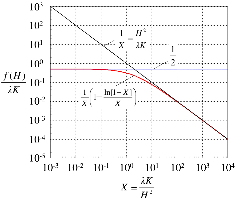
where $\lambda$ is considered to be positive, i.e., $\lambda>0$. Dividing Eq. (37) by $\lambda K$, and applying Eq. (38), we have the normalized extra-driving term given by

$$\frac{f(H)}{\lambda K}=\frac{1}{X}\left(1-\frac{\ln[1+X]}{X}\right).$$ (39)

To observe the properties of $f(H)$, the normalized term is plotted in Fig. 1. Consequently, $f(H)/(\lambda K)$ gradually approaches $1/2$ with decreasing $X$, while it approaches a common curve with increasing $X$. Therefore, we focus on two specific conditions, $X\leq 1$ and $X\gg 1$. Under the two conditions, the approximate formulas are given mathematically by

$$\ln[1+X]\approx X-\frac{X^{2}}{2}+\cdots\quad(X\leq 1),$$ (40)

$$\frac{\ln[1+X]}{X}\approx 0\quad(X\gg 1).$$ (41)

High-order terms have been neglected in Eq. (40). Substituting Eqs. (40) and (41), respectively, into Eq. (39), we have

$$\frac{f(H)}{\lambda K}\approx\begin{cases}\frac{1}{2}&(X\leq 1),\\ \frac{1}{X}&(X\gg 1).\\ \end{cases}$$ (42)

From Eqs. (38) and (42), $f(H)$ can be written as

$$f(H)\approx\begin{cases}\frac{\lambda K}{2}&(\frac{\lambda K}{H^{2}}\leq 1),\\ H^{2}&(\frac{\lambda K}{H^{2}}\gg 1).\\ \end{cases}$$ (43)

The constant-like and $H^{2}$-like terms are respectively obtained from each condition, as shown in Eq. (43). The constant-like term, $\lambda K/2$, can be interpreted as a kind of cosmological constant, although the specific condition $\lambda K/H^{2}\leq 1$ is required. In the next section, we discuss the constant-like term and the specific condition.

As a matter of fact, the extra driving term (which behaves like effective dark energy) can be derived even if dark energy is not assumed, i.e., even when $p=0$. Alternatively, the modified Rényi entropy is assumed in the present paper. In this sense, the original holographic equipartition law is modified. This modification is expected to provide new insights into cosmological models based on the holographic equipartition law.

As shown in Eq. (43), $H^{2}$-like terms are derived under a specific condition. However, the driving term is not likely to be related to the inflation of the early universe, because higher exponents terms such as $H^{4}$ terms should be required for the inflation Koma9 . In $\Lambda(t)$CDM models, the higher exponents terms have been closely examined in Ref. Sola_2015_2 . In entropic cosmology, quantum corrected entropy is introduced for the higher exponents terms, see, e.g., Ref. Tu2015 and the second paper of Ref. Easson12 .

VI Constant-like term under a specific condition

The acceleration equation can be derived from the holographic equipartition law with the modified Rényi entropy, as examined in the previous section. Interestingly, an extra driving term included in the equation is found to be constant-like under a specific condition. In this section, we discuss the constant-like term under the specific condition. To this end, the present cosmological model is reviewed, assuming that it is a particular case of $\Lambda(t)$CDM models. Substituting $\Lambda(t)/3=f(H)$ into Eqs. (1), (2), and (4), we obtain the Friedmann, acceleration, and continuity equations written as

$$H^{2}=\frac{8\pi G}{3}\rho+f(H),$$ (44)

$$\frac{\ddot{a}}{a}=-\frac{4\pi G}{3}\left(\rho+\frac{3p}{c^{2}}\right)+f(H),$$ (45)

$$\dot{\rho}+3\frac{\dot{a}}{a}\left(\rho+\frac{p}{c^{2}}\right)=-\frac{3\dot{f}(H)}{8\pi G},$$ (46)

where the extra driving term $f(H)$ is given by

$$f(H)=H^{2}\left(1-\frac{\ln[1+(\lambda K/H^{2})]}{\lambda K/H^{2}}\right),$$ (47)

and $K$ is

$$K=\frac{\pi k_{B}c^{5}}{\hbar G}=\frac{\pi k_{B}c^{2}}{L_{p}^{2}}.$$ (48)

As shown in Eq. (46), the right-hand side of the continuity equation is not zero generally. This non-zero right-hand side may be interpreted as the interchange of energy between the bulk (the universe) and the surface (the horizon of the universe) Lepe1 ; Koma9 . (The previous works of Solà et al. Sola_2015L14 ; Sola_2016_1 imply that the value of the non-zero right-hand side of the continuity equation should be small in $\Lambda(t)$CDM models Koma9 .) In the following, the right-hand side of the continuity equation is zero, because $f(H)$ is considered to be constant under a specific condition. General solutions for the present model, which includes a logarithmic term, are separately discussed in Appendix A.

This paper focuses on the constant-like term under a specific condition. From Eq. (43), the constant-like term and the specific condition can be written as

$$f(H)\approx\frac{\lambda K}{2}=\left(\frac{\lambda K}{2H_{0}^{2}}\right)H_{0}^{2}\quad\quad\left(\frac{\lambda K}{H^{2}}\leq 1\right),$$ (49)

where $H_{0}$ is the Hubble parameter at the present time and $\lambda K/(2H_{0}^{2})$ is a dimensionless constant (corresponding to $\alpha_{4}$ in Ref. Koma6 ). Hereafter, we call the constant-like term the constant term. Under the specific condition given by Eq. (49), the Friedmann, acceleration, and continuity equations are written as

$$H^{2}=\frac{8\pi G}{3}\rho+\left(\frac{\lambda K}{2H_{0}^{2}}\right)H_{0}^{2},$$ (50)

$$\frac{\ddot{a}}{a}=-\frac{4\pi G}{3}\left(\rho+\frac{3p}{c^{2}}\right)+\left(\frac{\lambda K}{2H_{0}^{2}}\right)H_{0}^{2},$$ (51)

$$\dot{\rho}+3\frac{\dot{a}}{a}\left(\rho+\frac{p}{c^{2}}\right)=0.$$ (52)

The three equations are essentially the same as those in the standard $\Lambda$CDM model. Setting $p=0$ for non-relativistic matter, the background evolution of the universe is analytically given by

$$\left(\frac{H}{H_{0}}\right)^{2} =\left(1-\frac{\lambda K}{2H_{0}^{2}}\right)\left(\frac{a}{a_{0}}\right)^{-3}+\frac{\lambda K}{2H_{0}^{2}}$$

$$=\left(1-\Omega_{h}\right)\left(\frac{a}{a_{0}}\right)^{-3}+\Omega_{h},$$ (53)

where $a_{0}$ represents the scale factor at the present time and $\Omega_{h}$ is a holographic parameter defined by

$$\Omega_{h}\equiv\frac{\lambda K}{2H_{0}^{2}}.$$ (54)

Using Eq. (54) and $\tilde{H}\equiv H/H_{0}$, Eq. (38) can be written as

$$X\equiv\frac{\lambda K}{H^{2}}=\frac{\frac{2\lambda K}{2H_{0}^{2}}}{H^{2}/H_{0}^{2}}=\frac{2\Omega_{h}}{\tilde{H}^{2}}\quad\quad(>0).$$ (55)

In the present model, the constant term $\lambda K/2$ and the holographic parameter $\Omega_{h}$ have been restricted by the inequality given in Eq. (49). Accordingly, the constraint on both $\lambda K/2$ and $\Omega_{h}$ can be discussed, without tuning.

In the history of an expanding universe, $H_{0}$ is expected to be the minimum value of $H$, because $r_{H}$ increases with time and $H$ is given by $H=c/r_{H}$ from Eq. (6). Therefore, when $H=H_{0}$, the most severe constraint on $\lambda K$ can be obtained from the inequality of Eq. (49). The constraint is written as

$$\lambda K\lessapprox H_{0}^{2}.$$ (56)

In the present model, Eq. (56) is mathematically required to obtain the constant term. From Eq. (56), the order of the constant term, $\lambda K/2$, is approximately given by

$$O\left(\frac{\lambda K}{2}\right)\lessapprox O\left(H_{0}^{2}\right),$$ (57)

or equivalently, from Eqs. (54) and (56), the order of $\Omega_{h}$ can be approximately written as

$$O\left(\Omega_{h}\right)=O\left(\frac{\lambda K}{2H_{0}^{2}}\right)\lessapprox O\left(1\right).$$ (58)

We now compare the constant term $\lambda K/2$ in the present model and the cosmological constant term $\Lambda/3$ in the standard $\Lambda$CDM model. In the $\Lambda$CDM model, the density parameter $\Omega_{\Lambda}$ for the cosmological constant $\Lambda$ is given by

$$\Omega_{\Lambda}\equiv\frac{\Lambda}{3H_{0}^{2}}.$$ (59)

Numerous cosmological observations indicate that the order of $\Omega_{\Lambda}$ is expected to be $1$, e.g., $\Omega_{\Lambda}=0.692$ from the Planck 2015 results Planck2015 . Accordingly, the order of $\Omega_{\Lambda}$ can be approximately written as

$$O\left(\Omega_{\Lambda}\right)\approx O\left(1\right).$$ (60)

Using Eqs. (59) and (60), we have

$$O\left(\frac{\Lambda}{3}\right)=O\left(\Omega_{\Lambda}H_{0}^{2}\right)\approx O\left(H_{0}^{2}\right).$$ (61)

Equations (57) and (61) imply that the order of the constant term $\lambda K/2$ is consistent with the order of $\Lambda/3$. That is, interestingly, the constant term in the present model is naturally consistent with the order of $\Lambda$ measured by cosmological observations as if it is $\Lambda$. Similarly, from Eqs. (58) and (60), the order of $\Omega_{h}$ is likely consistent with the order of $\Omega_{\Lambda}$. Of course, in the present model, $\lambda K\lessapprox H_{0}^{2}$ is required to obtain the constant term, assuming the modified Rényi entropy instead of the Bekenstein–Hawking entropy. This extension may be beyond the original holographic equipartition law. However, the constant term and the specific condition considered here may provide new insights into the cosmological constant problem.

Equation (56) can be written as $\lambda\lessapprox L_{p}^{2}/(\pi k_{B}r_{H0}^{2})$ using Eq. (48) and $H_{0}=c/r_{H0}$, where $r_{H0}$ is the Hubble horizon at the present time. This constraint indicates that $\lambda$ is an extremely small positive value. In other words, the modified Rényi entropy is approximately equivalent to the Bekenstein–Hawking entropy although it slightly deviates from the Bekenstein–Hawking entropy. Accordingly, the present model may imply that the cosmological constant is related to a small deviation from the Bekenstein–Hawking entropy. As time passes, the constraint is expected to be more severe because $r_{H0}$ increases with time. Consequently, the extra driving term in the present model should gradually deviate from the constant value, even if the severe condition is satisfied at the present time. That is, the present model can be distinguished from the $\Lambda$CDM model, as discussed in Appendix A.

In this paper, we have focused on the derivation of an extra driving term from the holographic equipartition law with the modified Rényi entropy. The obtained term $f(H)$ given by Eq. (47) is a logarithmic formula. However, under two specific conditions, it can be systematically written as $f(H)=C_{0}H_{0}^{2}+C_{1}H^{2}$, where $C_{0}$ and $C_{1}$ are dimensionless constants. In the $\Lambda(t)$CDM model, the above formula has been examined in detail Sola_2016_1 ; Valent2015 ; LimaSola_2013a ; Basilakos1-Sola_2014a . For example, Gómez-Valent et al. Valent2015 and Basilakos et al. Basilakos1-Sola_2014a have shown that it is not the $H^{2}$, $\dot{H}$, and $H$ terms but rather the constant term that plays an important role in cosmological fluctuations related to structure formations Koma9 . In addition, recently, $\Lambda(t)$CDM models, which include power series of $H$, have been found to be more suitable than the standard $\Lambda$CDM model Sola_2015L14 . In particular, the simple combination of the constant and $H^{2}$ terms, $f(H)=C_{0}H_{0}^{2}+C_{1}H^{2}$, is likely favored; see e.g., the works of Solà et al. Sola_2016_1 , Gómez-Valent et al. Valent2015 , and Lima et al. LimaSola_2013a , which indicate that $C_{0}$ is dominant and $C_{1}$ is expected to be small Sola_2015L14 ; Sola_2016_1 . The smallness of $C_{1}$ has not yet been explained by the holographic approach Koma9 , though it may be explained by a deeper understanding of the present model. For example, the logarithmic formula discussed in the present model slightly deviates from the constant value when $\lambda K/H^{2}\approx 1$, as shown in Fig. 1. Of course, this small deviation is not proportional to $H^{2}$. However, the small deviation may be related to the smallness of $C_{1}$, if the smallness can be interpreted as a deviation from a constant term. This task is left for future research.

Keep in mind that the present result depends on the choice of entropy. In this paper, the modified Rényi entropy Czinner1 ; Czinner2 is employed, in which the Bekenstein-Hawking entropy is considered to be a nonextensive Tsallis entropy. That is, the Bekenstein-Hawking entropy is assumed to satisfy the Tsallis composition rule. In addition, a logarithmic formula of the original Rényi entropy is used for the modified Rényi entropy Czinner1 ; Czinner2 , where the logarithmic formula is obtained from the Tsallis composition rule. For details of the modified Rényi entropy, see Refs. Czinner1 ; Czinner2 . The physical origin of the modified Rényi entropy is likely unclear at the present time. However, it is worthwhile to examine cosmological models based on the holographic equipartition law from various viewpoints. Note that the choice of temperature does not affect main results in the present study, because the extra driving term discussed here is related to $N_{\rm{sur}}=4S_{H}/k_{B}$ from Eq. (23) and is independent of the temperature C1 .

VII Conclusions

Recently, a novel type of Rényi entropy on a black-hole horizon was proposed by Biró and Czinner Czinner1 , in which a logarithmic formula of the original Rényi entropy was used and the Bekenstein–Hawking entropy was regarded as a nonextensive Tsallis entropy. In this study, the modified Rényi entropy has been applied to the holographic equipartition law proposed by Padmanabhan Padma2012A , to investigate cosmological models based on the holographic equipartition law. Consequently, the acceleration equation, which includes an extra driving term, can be derived in a homogeneous, isotropic, and spatially flat universe. The extra driving term is a logarithmic formula which can explain the accelerated expansion of the late universe, as for effective dark energy.

Under two specific conditions, the extra driving term is found to be the constant-like and $H^{2}$-like terms, respectively. In particular, when a specific condition is satisfied, the extra driving term is found to be constant-like, i.e., $\lambda K/2$, as if it is a cosmological constant $\Lambda$. In the present model, $\lambda K\lessapprox H_{0}^{2}$ is required to obtain the constant-like term from the most severe constraint. In other words, the constant-like term must be extremely small when the extra driving term behaves as if it is constant. The present model may imply that the cosmological constant is related to a small deviation from the Bekenstein–Hawking entropy. In addition, interestingly, the order of the constant-like term is naturally consistent with the order of the cosmological constant measured by observations, because the specific condition constrains the value of the constant-like term. The present model may provide new insights into the cosmological constant problem.

This paper focuses on the derivation of the extra driving term and the specific condition for the constant-like term. Accordingly, general solutions for the present model that includes a logarithmic driving term have been separately studied in Appendix A. To solve the cosmological equations, the present model is assumed to be a particular case of $\Lambda(t)$CDM models. From the obtained solution, the background evolutions of the universe in the present model are found to agree well with those in the standard $\Lambda$CDM model when both $2\Omega_{h}/\tilde{H}^{2}$ and $2\Omega_{h}$ are small. For lower redshift, the present model gradually deviates from the $\Lambda$CDM model, due to the logarithmic term. Therefore, the present model can be distinguished from the standard $\Lambda$CDM model.

Appendix A General Solutions for the present model and background evolutions of the late universe

So far, a constant term under a specific condition in the present model has been focused on, without tuning $\Omega_{h}$ given by Eq. (54). However, in general, the present model has a logarithmic driving term. Accordingly, in this Appendix, general solutions for the present model are examined, assuming that it is a particular case of $\Lambda(t)$CDM models. Using the solution, background evolutions of the late universe are briefly observed. In the following, $p$ is set to be zero for non-relativistic matter. In addition, $\Omega_{h}$ is considered to be a free constant parameter (i.e., a kind of density parameter for effective dark energy), as for $\Omega_{\Lambda}$ in the standard $\Lambda$CDM model.

A.1 General solutions for the present model

In this subsection, the general solution for the present model is examined. To this end, the present model is assumed to be a particular case of $\Lambda(t)$CDM models, as shown in Eqs. (44)–(46). From Eq. (47), the extra driving term $f(H)$ is written as

$$f(H)=H^{2}\left(1-\frac{\ln[1+(\lambda K/H^{2})]}{\lambda K/H^{2}}\right).$$ (62)

When $f(H)=\lambda K/2$, the solution is given by Eq. (53). The solution method for the present model is partially based on Refs. Koma4 ; Koma5 ; Koma6 . (When $f(H)$ is a power series of $H$ and $\dot{H}$, see e.g., the recent works of Gómez-Valent et al. Valent2015 and Basilakos et al. Basilakos1-Sola_2014a . )

Using $\ddot{a}/{a}=\dot{H}+H^{2}$, coupling Eq. (44) with Eq. (45) $\times 2$, and setting $p=0$, we obtain

$$\dot{H}+\frac{3}{2}H^{2}-\frac{3}{2}f(H)=0,$$ (63)

or, equivalently,

$$\dot{H}=-\frac{3}{2}H^{2}\left(1-\frac{f(H)}{H^{2}}\right).$$ (64)

From Eq. (64), we have $(dH/da)a$ given by

$$\left(\frac{dH}{da}\right)a =\left(\frac{dH}{dt}\right)\frac{dt}{da}a=-\frac{3}{2}H^{2}\left(1-\frac{f(H)}{H^{2}}\right)\frac{a}{\dot{a}}$$

$$=-\frac{3}{2}H^{2}\left(1-\frac{f(H)}{H^{2}}\right)\frac{1}{H}$$

$$=-\frac{3}{2}H\left(1-\frac{f(H)}{H^{2}}\right).$$ (65)

Substituting Eq. (62) into Eq. (65) gives

$$\left(\frac{dH}{da}\right)a =-\frac{3}{2}H\left(1-\frac{H^{2}\left(1-\frac{\ln[1+(\lambda K/H^{2})]}{\lambda K/H^{2}}\right)}{H^{2}}\right)$$

$$=-\frac{3}{2}H\left(\frac{\ln[1+(\lambda K/H^{2})]}{\lambda K/H^{2}}\right)$$

$$=-\frac{3}{2}H\left(\frac{\ln[1+(2\Omega_{h}/\tilde{H}^{2})]}{2\Omega_{h}/\tilde{H}^{2}}\right),$$ (66)

where the following equation given by Eq. (55) has been also used:

$$\frac{\lambda K}{H^{2}}=\frac{2\Omega_{h}}{\tilde{H}^{2}}.$$ (67)

Note that, from Eq. (54), $\Omega_{h}$ is defined by

$$\Omega_{h}\equiv\frac{\lambda K}{2H_{0}^{2}},$$ (68)

and the normalized Hubble parameter $\tilde{H}$ is defined as

$$\tilde{H}\equiv\frac{H}{H_{0}}.$$ (69)

Similarly, the normalized scale factor $\tilde{a}$ is defined as

$$\tilde{a}\equiv\frac{a}{a_{0}}.$$ (70)

Substituting $H=\tilde{H}H_{0}$ and $a=\tilde{a}a_{0}$ into Eq. (66), and arranging the resultant equation, we have

$$\left(\frac{d\tilde{H}}{d\tilde{a}}\right)\tilde{a}=-\frac{3}{2}\tilde{H}\left(\frac{\ln[1+(2\Omega_{h}/\tilde{H}^{2})]}{2\Omega_{h}/\tilde{H}^{2}}\right).$$ (71)

In addition, a parameter $N$ is defined by

$$N\equiv\ln\tilde{a},\quad\textrm{and therefore}\quad dN=\frac{d\tilde{a}}{\tilde{a}}.$$ (72)

Using Eq. (72), Eq. (71) can be written as

$$\left(\frac{d\tilde{H}}{dN}\right)=-\frac{3}{2}\tilde{H}\left(\frac{\ln[1+(2\Omega_{h}/\tilde{H}^{2})]}{2\Omega_{h}/\tilde{H}^{2}}\right).$$ (73)

When $\Omega_{h}$ is constant, Eq. (73) can be integrated as

$$\int\frac{d\tilde{H}}{\frac{3}{2}\tilde{H}\left(\frac{\ln[1+(2\Omega_{h}/\tilde{H}^{2})]}{2\Omega_{h}/\tilde{H}^{2}}\right)}=-\int dN.$$ (74)

This solution is given by

$$-\frac{1}{3}\textrm{li}\left(1+\frac{2\Omega_{h}}{\tilde{H}^{2}}\right)=-N+C=-\ln\tilde{a}+C,$$ (75)

where $C$ is an integral constant and ‘li’ represents the logarithmic integral LogInt defined as

$$\textrm{li}(x)\equiv\int^{x}_{0}\frac{dt}{\ln t}.$$ (76)

From Eqs. (69) and (70), the present values of $\tilde{H}$ and $\tilde{a}$ are $1$. Substituting $\tilde{H}=1$ and $\tilde{a}=1$ into Eq. (75), the integral constant $C$ can be written as

$$C=-\frac{1}{3}\textrm{li}\left(1+2\Omega_{h}\right).$$ (77)

Substituting Eq. (77) into Eq. (75), and solving the resultant equation with respect to $\tilde{a}$, we obtain

$$\tilde{a}=\left\{\exp\left[\textrm{li}\left(1+\frac{2\Omega_{h}}{\tilde{H}^{2}}\right)-\textrm{li}\left(1+2\Omega_{h}\right)\right]\right\}^{\frac{1}{3}}.$$ (78)

This equation is the general solution for the present model. The relationship between $\tilde{a}$ and $\tilde{H}$ for each $\Omega_{h}$ can be calculated from Eq. (78). Equations (78) and (53) approach the same approximate equation, respectively, when both $2\Omega_{h}/\tilde{H}^{2}\ll 1$ and $2\Omega_{h}\ll 1$ and when both $\Omega_{\Lambda}/\tilde{H}^{2}\ll 1$ and $\Omega_{\Lambda}\ll 1$. The two conditions, $2\Omega_{h}\ll 1$ and $\Omega_{\Lambda}\ll 1$, are related to the integral constants.

A.2 Background evolutions of the late universe

In this subsection, the background evolutions of the late universe in the present model are briefly examined. For this purpose, $\Omega_{h}$ is considered to be a free parameter. Note that, when Eq. (78) for $\Omega_{h}=0$ is calculated numerically, $\Omega_{h}$ is set to be $10^{-4}$.

To observe the properties of the present model, the luminosity distance is examined. The luminosity distance Sato1 is generally given by

$$\left(\frac{H_{0}}{c}\right)d_{L}=(1+z)\int_{1}^{1+z}\frac{dy}{F(y)},$$ (79)

where the integrating variable $y$, the function $F(y)$, and the redshift $z$ are given by

$$y=\tilde{a}^{-1},\hskip 5.69054ptF(y)=\tilde{H},\hskip 5.69054ptz\equiv\tilde{a}^{-1}-1.$$ (80)

The relationship between $\tilde{a}$ and $\tilde{H}$ for each $\Omega_{h}$ is obtained from Eq. (78). Using this relationship, the luminosity distance is calculated from Eqs. (79) and (80).

Figure 2: (Color online). Dependence of the luminosity distance $d_{L}$ on redshift $z$. The solid lines represent $d_{L}$ for the present model. The open diamonds with error bars are supernova data points taken from Ref. Riess2007SN1 . For the supernova data points, $H_{0}$ is set to $67.8$ km/s/Mpc from the Planck 2015 results Planck2015 .

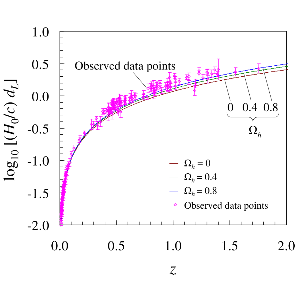
For typical results, the luminosity distances for $\Omega_{h}=0$, $0.4$, and $0.8$ are plotted in Fig. 2. The luminosity distance for the present model tends to be more consistent with supernova data points with increasing $\Omega_{h}$. This result indicates that the present model can describe an accelerated expansion of the late universe. However, the influence of the increase in $\Omega_{h}$ on $d_{L}$ is likely to be smaller than the influence of the increase in $\Omega_{\Lambda}$ in the $\Lambda$CDM model on $d_{L}$ (the result for the $\Lambda$CDM model is not shown). To compare the two models, a temporal deceleration parameter is examined.

The temporal deceleration parameter $q$ is defined by

$$q\equiv-\left(\frac{\ddot{a}}{aH^{2}}\right),$$ (81)

where positive $q$ represents deceleration and negative $q$ represents acceleration. It should be noted that the $q$ examined here is not the nonextensive parameter discussed in previous sections. Substituting Eq. (64) into $\ddot{a}/a=\dot{H}+H^{2}$, dividing the resultant equation by $-H^{2}$, and applying Eq. (81), we have

$$q=\frac{1}{2}-\frac{3}{2}\frac{f(H)}{H^{2}}.$$ (82)

In addition, substituting Eq. (62) into Eq. (82), and applying Eq. (67), we obtain

$$q =\frac{1}{2}-\frac{3}{2}\frac{f(H)}{H^{2}}=\frac{1}{2}-\frac{3}{2}\frac{H^{2}\left(1-\frac{\ln[1+(\lambda K/H^{2})]}{\lambda K/H^{2}}\right)}{H^{2}}$$

$$=\frac{1}{2}-\frac{3}{2}\left(1-\frac{\ln[1+(\lambda K/H^{2})]}{\lambda K/H^{2}}\right)$$

$$=-1+\frac{3}{2}\left(\frac{\ln[1+(2\Omega_{h}/\tilde{H}^{2})]}{2\Omega_{h}/\tilde{H}^{2}}\right).$$ (83)

The temporal deceleration parameter $q$ for the present model can be calculated from Eq. (83). Note that the relationship between $\tilde{a}$ and $\tilde{H}$ is obtained from Eq. (78).

For the $\Lambda$CDM model, substituting $f(H)=\Lambda/3$ into Eq. (82), and using $\Omega_{\Lambda}=\Lambda/(3H_{0}^{2})$ and $\tilde{H}=H/H_{0}$, we have

$$q=\frac{1}{2}-\frac{3}{2}\frac{\Omega_{\Lambda}}{\tilde{H}^{2}},$$ (84)

where $\tilde{H}^{2}$ is given by $\tilde{H}^{2}=(1-\Omega_{\Lambda})\tilde{a}^{-3}+\Omega_{\Lambda}$. In a flat universe, the density parameter $\Omega_{m}$ for matter is given by $\Omega_{m}=1-\Omega_{\Lambda}$, neglecting the density parameter for the radiation.

Figure 3: (Color online). Dependence of the temporal deceleration parameter $q$ on redshift $z$. The solid lines represent $q$ for the present model, while the symbols represent $q$ for the $\Lambda$CDM model. Note that positive $q$ represents deceleration and negative $q$ represents acceleration.

Figure 4: (Color online). Dependence of the parameter $2\Omega_{h}/\tilde{H}^{2}$ on redshift $z$. Note that $2\Omega_{h}/\tilde{H}^{2}$ is equivalent to $X\equiv\lambda K/H^{2}$ shown in Fig. 1.

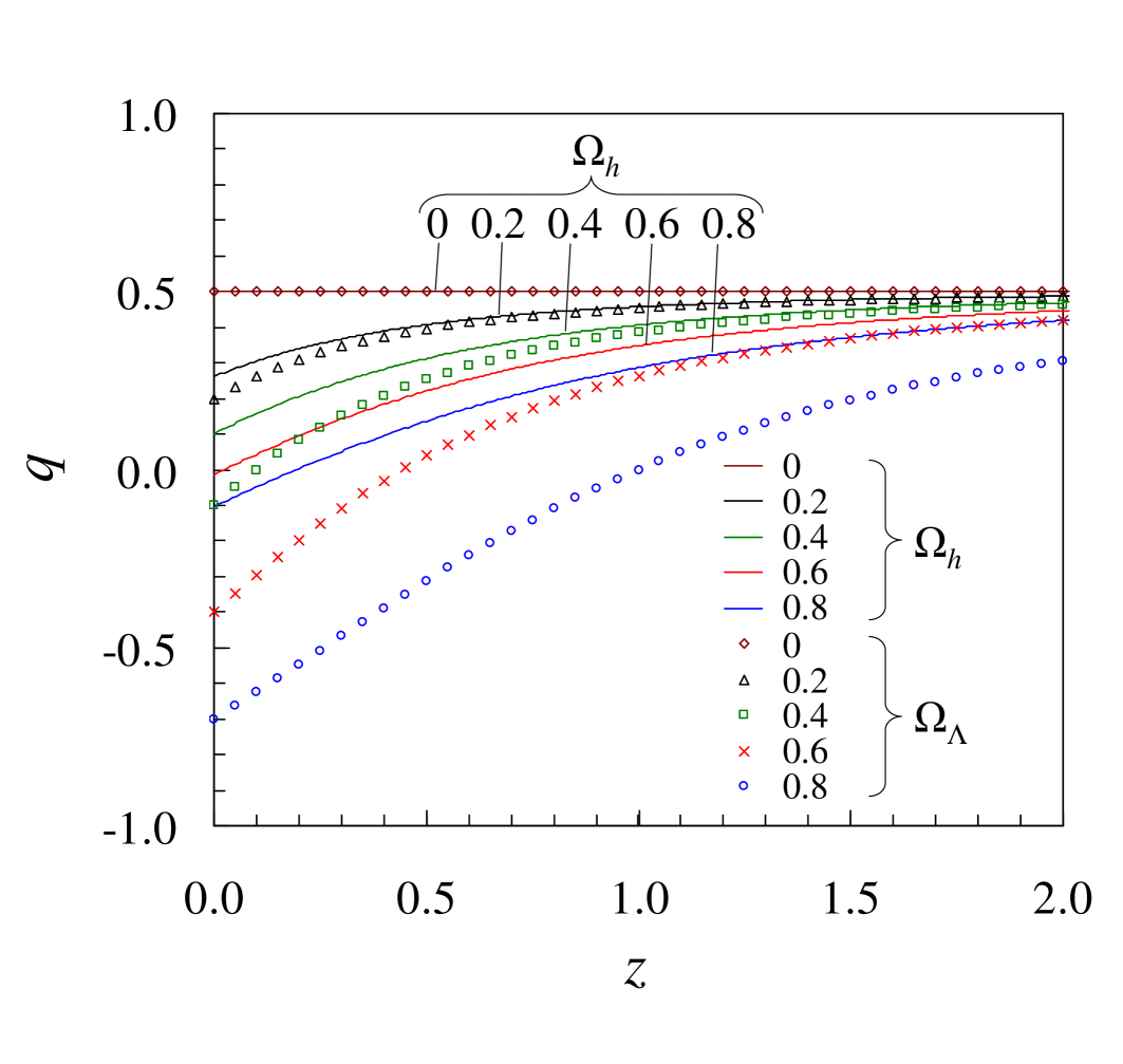
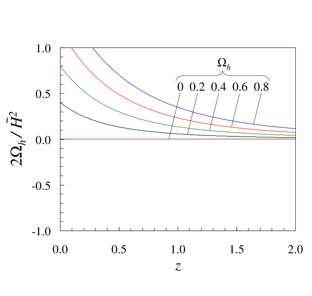
Figure 3 shows the dependence of the temporal deceleration parameter $q$ on the redshift $z$. As expected, $q$ for $\Omega_{h}=0$ and $0.2$ is consistent with that for $\Omega_{\Lambda}=0$ and $0.2$, respectively. However, $q$ for the present model gradually deviates from that for the $\Lambda$CDM model, with increasing $\Omega_{h}$, especially for low redshift. In fact, even for $\Omega_{h}=0.2$, $q$ gradually deviates from that for $\Omega_{\Lambda}=0.2$ with decreasing $z$, although the two results agree well for high redshift. As shown in Fig. 4, $2\Omega_{h}/\tilde{H}^{2}$ increases with decreasing $z$, because $\tilde{H}$ decreases with decreasing $z$. That is, the deviation from the $\Lambda$CDM model for low redshift (shown in Fig. 3) is related to the increase in $2\Omega_{h}/\tilde{H}^{2}$. In addition, for $\Omega_{h}=0.6$ and $0.8$, $q$ varies from positive to negative with decreasing $z$, as shown in Fig. 3. Therefore, the present model can describe a decelerated and accelerated expansion of the late universe.

In this Appendix, the general solution for the present model has been examined, assuming that the present model is a particular case of $\Lambda(t)$CDM models. In addition, background evolutions of the late universe in the present model have been discussed. Consequently, the present model is found to agree well with the standard $\Lambda$CDM model, when both $2\Omega_{h}/\tilde{H}^{2}$ and $2\Omega_{h}$ are small. For lower redshift, the present model gradually deviates from the $\Lambda$CDM model, due to the properties of the logarithmic driving term. Accordingly, the present model examined here can be distinguished from the $\Lambda$CDM model.