Pseudo-time regularization for PDE with solution-dependent diffusion

Abstract.

This work unifies pseudo-time and inexact regularization techniques for nonmonotone classes of partial differential equations, into a regularized pseudo-time framework. Convergence of the residual at the predicted rate is investigated through the idea of controlling the linearization error, and regularization parameters are defined following this analysis, then assembled in an adaptive algorithm. The main innovations of this paper include the introduction of a Picard-like regularization term scaled by its cancellation effect on the linearization error to stabilize the Newton-like iteration; an updated analysis of the regularization parameters in terms of minimizing an appropriate quantity; and, strategies to accelerate the algorithm into the asymptotic regime. Numerical experiments demonstrate the method on an anisotropic diffusion problem where the Jacobian is not continuously differentiable, and a model problem with steep gradients and a thin diffusion layer.

1. Introduction

This paper is concerned with the finite element approximation to second order quasilinear elliptic equations in divergence form,

$$-{\operatorname{div}}(\kappa(u)\nabla u) =f,\text{ in }\Omega$$ (1.1)

$$u =0,\text{ on }\partial\Omega,$$ (1.2)

for polygonal doman $\Omega\subset{\mathbb{R}}^{2}$. Nonlinear diffusion problems are ubiquitous throughout science and engineering applications, appearing in applications such as heat conduction, groundwater flow, diffusion of contaminants and flow in porous media [5, 8, 15, 19]. Here, the nonlinear diffusion coefficient $\kappa(u)$ may be thought of as a scalar quantity, or in the more general anisotropic case as a matrix coefficient with entries $\kappa_{ij}(u),~{}j=1,2$, where (1.1) has the expansion

$$-\sum_{i,j=1}^{n}\frac{\partial}{\partial x_{j}}\left(\kappa_{ij}(u)\frac{\partial}{\partial x_{j}}u\right)=f,\text{ in }\Omega,$$ (1.3)

with the ellipticity condition: For some $\eta>0$

$$\sum_{i,j=1}^{2}\kappa_{ij}(s)\xi_{i}\xi_{j}\geq\eta\sum_{i=1}^{2}\xi_{i}^{2},$$ (1.4)

for any $s\in{\mathbb{R}}$, and all $\xi=(\xi_{1},\xi_{2})\in{\mathbb{R}}^{2}$.

As remarked in [19], while (1.1) for scalar-valued $\kappa(u)$ may be solved by the Kirchhoff transform (see, e.g., [8]), this technique does not carry over to the anisotropic case, or to lower order solution-dependent terms. The nonlinear diffusion problem (1.1) is generally in the class of nonmonotone problems; that is $\int_{\Omega}\left\{\left(\kappa(v)\nabla v-\kappa(w)\nabla w\right)\cdot\nabla(v-w)\right\}>0$, is not guaranteed to hold for each $u,v$ is the solution space, e.g., $u,v\in H_{0}^{1}(\Omega)$. While convergence and optimality of finite element methods for monotone classes of quasilinear problems have been recently investigated in [3, 17], and the references therein, nonmonotone classes of problems are less understood. In particular, convergence results rely on sufficiently fine global mesh conditions, and sufficiently close initial guesses to assume convergence of Newton-iterations to solve the discrete nonlinear problem [4, 11, 18, 21]. Other recent work [14] includes this problem class in an adaptive framework of incomplete linear and nonlinear solves, but with the implicit assumption that the sequence of solution iterates is convergent to the solution. As described in previous work by the author in [25, 26, 27], the Newton iterations cannot realistically be assumed to converge, and are often observed to diverge, especially for problems of the form (1.1) which may contain steep gradients and thin internal layers in the solution-dependent diffusion coefficient $\kappa(u)$. The interest in the current investigation is to develop a regularized adaptive method and understand the residual convergence of the discrete nonlinear problem without these assumptions. It is of particular interest to allow a solution process to start on a coarse mesh which is refined adaptively, to uncover an efficient and accurate discretization. Future work will directly address convergence of the discrete solution to the weak solution of (1.1).

The weak form of (1.1)-(1.2) is given by: Find $u\in{\mathcal{U}}$ such that

$$B(u;u,v)=\int_{\Omega}fv,~{}\text{ for all }v\in{\mathcal{V}},$$ (1.5)

for solution space ${\mathcal{U}}$ and test space ${\mathcal{V}}$, with

$$B(u;u,v)=\int_{\Omega}\kappa(u)\nabla u\cdot\nabla v.$$ (1.6)

Based on the analysis of [12, 19, 29], the following set of conditions in addition to the uniform ellipticity (1.4) is sufficient to assure existence and uniqueness of the weak solution $u\in H_{0}^{1}(\Omega)$ of  (1.5).

Assumption 1.1.

Assume the data satisfy the following boundedness and Lipschitz conditions.

1. Boundedness of the diffusion coefficient

   $$\text{ess sup\,}_{s\in{\mathbb{R}}}\kappa_{ij}(s)\leq C_{\kappa},~{}i,j=1,2.$$ (1.7)

2. Boundedness of the source: $f\in L_{2}(\Omega)$ satisfies

   $$\text{ess sup\,}_{x\in\Omega}f(x)\leq C_{f}.$$ (1.8)

3. Lipschitz continuity of the diffusion coefficient

   $$|\kappa_{ij}(s)-\kappa_{ij}(t)|\leq\omega_{\kappa}|s-t|,~{}j=1,2,~{}\text{ for all }s,t\in{\mathbb{R}}.$$ (1.9)

For scalar-valued $\kappa$, the above should be interpreted with $\kappa_{11}=\kappa_{22}=\kappa$, and $\kappa_{12}=\kappa_{21}=0$.

A finite dimensional, or discrete problem corresponding to  (1.6), is given by: Find $u\in{\mathcal{U}}_{k}$ such that

$$B(u;u,v)=\int_{\Omega}fv,~{}\text{ for all }v\in{\mathcal{V}}_{k}\subset{\mathcal{V}},$$ (1.10)

where ${\mathcal{U}}_{k}\subset{\mathcal{U}}$ and ${\mathcal{V}}_{k}\subset{\mathcal{V}}$ are finite dimensional subspaces of the solution and test spaces. For the remainder of this paper, ${\mathcal{U}}$ and ${\mathcal{V}}$ are assumed subsets of $H_{0}^{1}(\Omega)$. The trial and test spaces ${\mathcal{U}}_{k}={\mathcal{V}}_{k}$, now referred to as ${\mathcal{V}}_{k}$, are taken as the $C^{0}$ continuous ${\mathcal{P}}^{p}$ finite element spaces of polynomials of degree $p$ over each mesh element, corresponding to nested mesh partitions, ${\mathcal{T}}_{k}$, which are conforming in the sense of  [6].

In the current discussion, a Newton-like method is applied so solve the discrete nonlinear equations induced by (1.10). The advantages of a Newton-like approach include fast convergence in the asymptotic regime, and the mesh-independence principle, as in for instance  [10]. To understand the convergence of sequence of linear equations used to approximate the solution of the discrete nonlinear problem, we require some control of the Jacobian. For this reason, the following conditions on the problem data are considered, in addition to those for well-posedness of the PDE, namely, the ellipticity condition (1.4) and Assumption 1.1.

Assumption 1.2 (Assumptions on the problem data).

The following assumptions are made on the diffusion coefficient $\kappa^{\prime}(u)$, componentwise, $\kappa_{ij}^{\prime}(u),~{}j=1,2$.

1. $\kappa^{\prime}$ is bounded. In particular

   $$\lVert{\kappa^{\prime}(s)\xi}\rVert\leq C_{B}\lVert{\xi}\rVert~{}\text{ for all }s\in{\mathbb{R}}~{}\text{ and }~{}\xi\in{\mathbb{R}}^{2}.$$ (1.11)

2. $\kappa^{\prime}$ satisfies the Lipschitz condition

   $$|\kappa_{ij}^{\prime}(s)-\kappa_{ij}^{\prime}(t)|\leq\omega_{B}|s-t|,~{}j=1,2,~{}\text{ for all }s,t\in{\mathbb{R}}.$$ (1.12)

Remark 1.3 (Standard problem classes).

The two existing convergence results for adaptive methods for nonmonotone problems of the form (1.1) are developed in  [21] using continuous Galerkin, in particular linear elements; and, [4] using discontinuous Galerkin methods.

The results of [21] are adapted from the analysis of uniform methods in [5]. Their approach assumes $W^{1,p}$, $p>2$ regularity of the solution $u$, and bounded $\kappa(s),\kappa^{\prime}(s)$ and $\kappa^{\prime\prime}(s)$ for all $s\in{\mathbb{R}}$. The results of  [4] are adapted from the analysis of uniform methods in [18], based on the results of [11]. For these results, it is assumed that the solution $u\in H^{2}(\Omega)\cap W^{1,\infty}(\Omega)$, and $\kappa(s)$ is twice continuously differentiable with bounded $\kappa(s),\kappa^{\prime}(s)$ and $\kappa^{\prime\prime}(s)$ for all $s\in{\mathbb{R}}$.

Both frameworks explicitly assume a uniformly small initial meshsize and either implicitly or explicitly assume the convergence of the iterative method used to solve the discrete nonlinear system on each refinement.

The following notation is used throughout the paper. Where not otherwise specified, the norm $\lVert{\cdot}\rVert$ denotes the $L_{2}$ norm. The integral $\int_{\Omega}uv$ is sometimes denoted $(u\,,v)$; and, $\langle z,w\rangle$ denotes a Euclidean product between vectors $z$ and $w$.

The remainder of the paper is structured as follows. Section 2 describes a framework for pseudo-time regularization, exploiting the quasi-linear structure of (1.5), and specifies the regularized system under inexact assembly. Section 3 derives the expansion of the latest residual in terms of the previous residual, exposing the regularization and linearization error terms. Section 4 suggests a set of regularization parameter updates based on the representation of Section 3, together with an adaptive algorithm. Finally, Section 5 demonstrates the ideas with some numerical experiments.

2. Regularized formulation

The regularization framework is next described. First, an error decomposition is discussed to separate out the contributions to the error in each iterate; that is, each solution to a linearized problem used to approximate the solution to (1.5). The contributions to the error include those induced from added regularization, linearization, early termination of the iterations, inexact assembly, and discretization.

Then, in Section 2.2, a pseudo-time regularized iteration is described and fit into this framework. First, the pseudo-time regularization is introduced in a general sense, then the regularized iteration is derived from a linearization of the abstract formulation of the discrete problem (1.10). Section 2.3, then introduces notation for the inexact assembly of the discrete problem, leading to the regularized iteration in matrix form. The steps are separated out in this presentation to emphasize the relation between the practical inexactly assembled equation that is actually solved computationally, and the abstract formulation of the problem that is thought of on the PDE level.

2.1. Error decomposition

The goal of the numerical method, finite element or otherwise, is to approximate the PDE solution; in this case, the solution to (1.5). The error may be understood by breaking it into components describing the discretization error, quadrature error, and so-called linearization or nonlinear iteration error. In the following notation, $u$ represents the (or a) solution to (1.5); and $u_{k}^{{\mathcal{E}},\ast}$ denotes the solution to the discrete nonlinear problem on the $k^{th}$ refinement of the initial mesh partition, under exact assembly. Neither $u$ nor $u_{k}^{{\mathcal{E}},\ast}$ are generally computable quantities. The iterate $u_{k}^{\ast}$ is the solution up to some set tolerance of the discrete problem using a numerical and potentially inexact assembly procedure; $u_{k}^{\ast}$ may or may not be computable. In terms of the inexactly assembled problem, $u_{k}$ is the terminal iterate, potentially before convergence to tolerance, and $u_{k}^{n}$ is the $n^{th}$ iterate on the $k^{th}$ refinement.

$$u-u_{k}^{n}=(u-u_{k}^{{\mathcal{E}},\ast})+(u_{k}^{{\mathcal{E}},\ast}-u_{k}^{\ast})+(u_{k}^{\ast}-u_{k})+(u_{k}-u_{k}^{n}).$$ (2.1)

The frameworks developed in [4, 21] show convergence to zero of the first term of (2.1), for a restricted class of problems of the type (1.1) (see Remark 1.3), under the assumptions of a sufficiently small meshsize. These asymptotic results motivate the current work, by demonstrating the approximation properties of a finite element solution to the PDE solution; however, the goal now is to develop a computational framework for which $u_{k}^{{\mathcal{E}},\ast}\rightarrow u$ still holds, and by which $u_{k}^{{\mathcal{E}},\ast}$ can be approximated by a computable sequence.

To that end, a regularized iteration is introduced starting on the initial, presumably coarse, mesh. The expansion of the error incorporating the introduced regularization breaks the last term of (2.1) into two new terms. Let $u_{k}^{S}$ be the terminal iterate of the regularized problem on refinement $k$. For ease of notation, the indices on $S$ are suppressed, however it should be understood that $u_{k}^{S}$ is subject to regularization $S_{k}$; and likewise, on iteration $n$ of refinement $k$, the iterate $u_{k}^{S,n}$ is subject to regularization $S_{k}^{n}$.

$$u-u_{k}^{S,n}=(u-u_{k}^{{\mathcal{E}},\ast})+(u_{k}^{{\mathcal{E}},\ast}-u_{k}^{\ast})+(u_{k}^{\ast}-u_{k})+(u_{k}-u_{k}^{S})+(u_{k}^{S}-u_{k}^{S,n}).$$ (2.2)

The regularization addressed in this paper can be broken into two parts: a Jacobian regularization and a residual regularization term. Then the regularized Newton-like iteration described in the following sections can be written in terms of a standard Newton iteration for this problem with Jacobian $J=J(u)$ and residual $r=r(u)$, $Jw=r,~{}u\leftarrow u+w$, by

$$(J+S^{J})w=r+S^{res},\quad u\leftarrow u+w.$$ (2.3)

Denoting $S=S^{J}+S^{res}$, eliminating the regularization from the iteration can be described as sending $S\rightarrow 0$.

Control of the last term of (2.2), $(u_{k}^{S}-u_{k}^{S,n})$ requires assumptions on the PDE, for instance Assumption 1.2, as well as assumptions on the regularization; essentially, the sequence of regularized linear problems must be sufficiently stable.

Due to the regularization structure (2.3), control of the fourth term $(u_{k}-u_{k}^{S})$ is established by $S\rightarrow 0$ for all $k\geq K_{0}$, for some iteration $K_{0}$. If the problem (1.5) is sufficiently well-posed, then the regularized iteration should limit and indeed revert to a standard Newton-iteration on each refinement after some level $K_{0}$. This type of result is detailed for a similar regularized Newton-like method in [27]. It is noted however that sending $S^{res}\rightarrow 0$ restores consistency of the iteration. If a problem features a potentially indefinite or badly conditioned Jacobian in the vicinity of a solution, it may be beneficial not to send $S^{J}$ to zero, rather to keep some background level of Jacobian regularization that does not interfere with the convergence of the iteration.

The third term of (2.2) is the difference between the terminal iterate and one converged to tolerance. This term is zero for $k$ larger than some $K_{1}$, where $K_{1}$ may be close and potentially equal to $K_{0}$, under a suitable residual-reduction condition for terminating the nonlinear iterations on each refinement level $k$. In the early stages of the solution process however, the nonlinear iteration may be stopped far from convergence, and the difference $(u_{k}^{\ast}-u_{k})$ may be non-negligible.

The second term of (2.2) describes the error induced by inexact integration. With the potential of a highly oscillatory diffusion coefficient in (1.1), this error term is not automatically assumed to be small as it is in [4, 21] and the references therein, where the assumption of a sufficiently small global meshsize can control the level of accuracy. Generally, information can be lost both by the averaging of integration against basis functions, and by the secondary averaging of approximate integration by quadrature. Finally, the first term $u-u_{k}^{{\mathcal{E}},\ast}$ constitutes the discretization error, the difference between a solution to (1.5) and the solution of the exactly assembled discrete nonlinear problem on refinement $k$. The analysis of these first two terms, determining convergence of the error, is beyond the scope of this paper, which analyzes efficient convergence of the residual. The conditions under which $u_{k}^{\ast}$ converges to $u$ for $k$ greater than some $K_{2}$ will be discussed elsewhere.

Remark 2.1 (Inexact linear solves).

Solving the linear equations by an iterative method yields yet another term in the expansion. For linear iteration $l$, the error between the PDE solution $u$ and iteration $l$, of regularized linear solve $n$, on mesh refinement $k$, may be decomposed into

$$u-(u_{k}^{n})^{l} =(u-u_{k}^{{\mathcal{E}},\ast})+(u_{k}^{{\mathcal{E}},\ast}-u_{k}^{\ast})+(u_{k}^{\ast}-u_{k})+(u_{k}-u_{k}^{S})+(u_{k}^{S}-u_{k}^{S,n})$$

$$+(u_{k}^{S,n}-(u_{k}^{S,n})^{l}).$$ (2.4)

The last error term is not addressed in the current paper, and the linear systems are assumed solved exactly. It is noted however that incomplete linear solves can be exploited for both their regularization properties and efficiency, and this topic is worth investigation.

2.2. Regularized abstract formulation

The regularized linear equations compatible with error decomposition (2.2) are now derived through a pseudo-time discretization framework with respect to the abstract discrete problem (1.10). The pseudo-time framework developed in for instance [2, 7, 22], the book [9], and the references therein, suggests to stabilize the solution of the elliptic equation $F(u)=0$, introduce the pseudo-time dependence to $u$, and solve $\partial u/\partial t+F(u)=0$. To allow a preconditioned or more general regularized framework, the discrete nonlinear pseudo-time regularized problem is: Find $u\in{\mathcal{V}}_{k}\subset{\mathcal{V}}$ such that

$$\phi(\dot{u},v)+B(u;u,v)=\int_{\Omega}fv,\text{ for all }v\in{\mathcal{V}}_{k},$$ (2.5)

where $\dot{u}=\partial u/\partial t$. Here, it is assumed that the bilinear form $\phi(\cdot\,,\cdot\,)$ is continuous with respect to the native norm ${\mathcal{V}}$, in this case taken to be the $H^{1}$ norm.

$$\phi(w,v)\leq C_{\phi}\lVert{w}\rVert_{1}\lVert{v}\rVert_{1}.$$ (2.6)

The continuity assures $\phi(\dot{u},\cdot)$ decays to zero as $\dot{u}\rightarrow 0$ indicating a steady state solution. Rather that coercive, $\phi$ is assumed semi-definite

$$\phi(w,w)\geq 0.$$ (2.7)

This allows for a more general regularization, as used in [25, 26], in which a cutoff function is used to only allow the regularization to act on select degrees of freedom. Upon matrix assembly, the role of $\phi$ can be viewed as improving the condition of the approximate Jacobian, and it should be chosen with this in mind. In the numerical experiments of Section 5, two different choices of $\phi$ are illustrated. The first sets $\phi(w,v)=((1+|\kappa^{\prime}(z)|)\nabla w,\nabla v)$, for $z$ the initial solution iterate on each refinement, thus adding more regularization locally to control steeper gradients in the diffusion. The second uses $\phi(w,v)=(\nabla w,\nabla v)$, the standard Laplacian preconditioner, adding a uniform level of diffusion to stabilize the Jacobian. The regularization functional is left in general form for the remainder of the analysis to emphasize that these are two of many choices.

A generalization of the Newmark time integration strategy  [24], exploiting the structure of the quasilinear equation (1.1) is now introduced to discretize (2.5) in pseudo-time

$$\phi({(\Delta t^{n}})^{-1}w^{n},v)=-\widetilde{\gamma}_{00}B(u^{n};u^{n},v)-\widetilde{\gamma}_{10}B(u^{n+1},u^{n},v)-\widetilde{\gamma}_{01}B(u^{n},u^{n+1},v)+(f,v),$$ (2.8)

where $(f,v)=\int_{\Omega}fv,$ and $w^{n}=u^{n+1}-u^{n}$. Linearizing the second term on the right, and rewriting the third to isolate the dependence on $w^{n}$ yields

$$\phi({(\Delta t^{n}})^{-1}w^{n},v) =-\widetilde{\gamma}_{00}B(u^{n};u^{n},v)-\widetilde{\gamma}_{10}\left(B(u^{n},u^{n},v)+B_{1}^{\prime}(u^{n};u^{n},v)(w^{n})\right)$$

$$\quad-\widetilde{\gamma}_{01}\left(B(u^{n},u^{n},v)+B(u^{n},w^{n},v)\right)+(f,v),$$ (2.9)

where $B_{1}^{\prime}(u;z,v)(w)\coloneqq\frac{d}{ds}B(u+sw;z,v)\big{|}_{s=0}$, the Gateaux derivative in the first argument of $B$, in the direction $w$. Rearranging (2.2) so that all terms involving the update step $w^{n}$ appear on the left, and rescaling by $\widetilde{\gamma}\coloneqq\widetilde{\gamma}_{00}+\widetilde{\gamma}_{10}+\widetilde{\gamma}_{01},$ yields

$$\alpha^{n}\phi(w^{n},v)+\gamma_{10}B_{1}^{\prime}(u^{n};u^{n},v)(w)+\gamma_{01}B(u^{n};w^{n},v)=-B(u^{n};u^{n},v)+\delta(f,v),$$ (2.10)

with the four regularization coefficients given by

$$\alpha^{n}=1/({\Delta t^{n}}\cdot{\widetilde{\gamma}}),\quad\gamma_{10}={\widetilde{\gamma}_{10}}/{\widetilde{\gamma}},\quad\gamma_{01}={\widetilde{\gamma}_{01}}/{\widetilde{\gamma}},\quad\text{ and }\quad\delta=1/{\widetilde{\gamma}}.$$ (2.11)

The coefficient $\alpha^{n}$ is then the rescaled reciprocal of the pseudo-time step, and $\alpha^{n}\rightarrow 0$, corresponds to $\Delta t^{n}\rightarrow\infty$. It is remarked that $\gamma_{10}=\gamma_{01}$ corresponds to the method discussed in [26], where this parameter is taken greater than one to introduce an increase in numerical dissipation, or controlled damping, into the iteration. Further, $\gamma_{01}=1=\gamma_{10}$ corresponds to an implicit, or backward Euler discretization of (2.5); while $\gamma_{01}=0=\gamma_{10}$, corresponds to an explicit, or forward Euler discretization of (2.5). And finally, $\gamma_{01}=1$ and $\gamma_{10}=0$ leads to a Picard iteration. It is also recognized that $\delta=1$ yields a consistent pseudo-time discretization.

2.3. Inexact assembly

Both the finite dimensional equation (1.10), and the pseudo-time regularized (2.5), are abstract equations rather than computable systems. To clarify which quantities are assumed computationally available, the following notation is introduced to describe the discrete system induced inexact assembly, e.g by quadrature, which may be assumed inexact for nonpolynomial integrands. Let ${\mathcal{V}}$ be a discrete space, here a finite element space, with $n_{dof}$ degrees of freedom, spanned by the basis functions $\{\varphi^{j}\}_{j=1}^{n_{dof}}$. Supposing $u,v,w,z\in{\mathcal{V}}$, each function has an exact expansion as a linear combination of basis functions; in particular $w=\sum_{j=1}^{n_{dof}}\tt w_{j}\varphi^{j},$ with $\tt w$ the vector of coefficients ${\tt w}_{j},~{}j=1,\ldots,n_{dof}$. Let $A(u;z)$ be an inexact assembly of $B(u;z,\varphi^{j}),~{}j=1,\ldots,n_{dof}$, with an error introduced by inexact integration, e.g., quadrature error. The source vector $f_{Q}$ is formed by the inexact integral of source function $f$ against each basis function $\varphi^{j}$. The matrix assembly of the regularization $\phi(w,\varphi^{j})$ is denoted $R$. Let ${\mathcal{A}}_{Q}$ represent the inexact assembly operator. The assembled systems under ${\mathcal{A}}_{Q}$ are denoted as follows.

$$A(u;z) \coloneqq{\mathcal{A}}_{Q}\left\{(B(u;z,\varphi^{j})\right\}_{j=1}^{n_{dof}},$$ (2.12)

$$A_{1}^{\prime}(u;z)\tt w \coloneqq{\mathcal{A}}_{Q}\left\{\frac{d}{dt}B(u+tw;z,\varphi^{j})\big{|}_{t=0}\right\}_{j=1}^{n_{dof}},$$ (2.13)

$$A_{2}^{\prime}(u)\tt w \coloneqq{\mathcal{A}}_{Q}\left\{\frac{d}{dt}B(u;z+tw,\varphi^{j})\big{|}_{t=0}\right\}_{j=1}^{n_{dof}}=A(u,w),$$ (2.14)

$$R{\tt w} \coloneqq{\mathcal{A}}_{\mathcal{E}}\left\{\phi(w,\varphi^{j})\right\}_{j=1}^{n_{dof}},$$ (2.15)

$$f_{Q} \coloneqq{\mathcal{A}}_{Q}\left\{\int f\varphi^{j}\right\}_{j=1}^{n_{dof}}.$$ (2.16)

The following commuting diagram holds for the discrete assembly procedure given by (2.12)-(2.13), with $u,v,w,z\in{\mathcal{V}}$. That is, the inexact assembly operator ${\mathcal{A}}_{Q}$ commutes with the Gateaux derivative of the first argument of $B(\cdot\,,\cdot\,,\cdot\,)$.

$$B(u;z,v) \underrightarrow{\qquad{\mathcal{A}}_{Q}\qquad} A(u;z)$$

$${\small\partial_{u}}\Bigg{\downarrow} {\small\partial_{u}}\Bigg{\downarrow}$$

$$B_{1}^{\prime}(u;z,v)(w) \underrightarrow{\qquad{\mathcal{A}}_{Q}\qquad} A_{1}^{\prime}(u;z)\tt w,$$ (2.17)

This justifies the use of Taylor’s theorem in the error representation of the residual in Section 3. In general, the Gateaux derivative commutes with projection-type discretizations; see for example [20]. This includes assembly under inexact integration, assuming the integral approximation over each element $T$ falls in the general form $\int_{T}\phi\approx\sum_{i=1}^{n_{Q_{T}}}\phi(x_{i})\rho_{i}$, for $n_{Q_{T}}$ points $x_{i}$ in the interior of element $T$, and weights $\rho_{i}$.

2.4. Regularized matrix equations

Processing the linear pseudo-time regularized equation (2.10) with the inexact assembly given by (2.12)-(2.16), yields the coefficients of the update step $w$ as the solution to a linear system of equations.

$$\left\{\alpha^{n}R+\gamma_{10}A_{1}^{\prime}(u^{n};u^{n})+\gamma_{01}A_{2}^{\prime}(u^{n})\right\}{\tt w}^{n}=\delta f_{Q}-A(u^{n};u^{n}),$$ (2.18)

which may be written as

$$M^{n}{\tt w}^{n} =\frac{1}{\gamma_{10}}r^{n},~{}\text{ with}~{}$$ (2.19)

$$M^{n} =\frac{1}{\gamma_{10}}\alpha^{n}R+A_{1}^{\prime}(u^{n};u^{n})+(1+\sigma_{01}^{n})A_{2}^{\prime}(u^{n}),\quad\sigma_{01}=\frac{\gamma_{01}}{\gamma_{10}}-1,$$ (2.20)

$$r^{n} =\delta f_{Q}-A(u^{n};u^{n}),$$ (2.21)

with the update $u^{n+1}=u^{n}+w^{n}$.

With respect to (2.3), the formal representation of the regularization structure, the Jacobian part $S^{J}$, and the residual part $S^{res}$, of the regularization are given by

$$S^{J} =\alpha R+(\gamma_{10}-1)A_{1}^{\prime}(u^{n};u^{n})+(\gamma_{01}-1)A_{2}^{\prime}(u^{n}),~{}\text{ and }$$ (2.22)

$$S^{res} =(\delta-1)f_{Q}.$$ (2.23)

Consistency is restored by sending regularization parameter $\delta\rightarrow 1$. Asymptotic efficiency is restored by sending $\alpha\rightarrow 0$, $\gamma_{10}\rightarrow 1$ and $\gamma_{01}\rightarrow 1$, although this asymptotic efficiency may be at least partially sacrificed for stability, even into the asymptotic regime, where the iterations converge to tolerance. This balance is understood in the next section where the residual representation exposes the error contributions from regularization and linearization. So long as the regularization effectively controls the linearization error without increasing the norm of the residual, it is viewed as beneficial.

3. Residual representation of the matrix equation

The residual representation follows the standard method of applying Taylor’s theorem to expand the $(n+1)^{th}$ residual about the $n^{th}$ residual, justified by the commuting diagram (2.3). This exposes the separate terms from the introduced regularization error and the intrinsic linearization error. The linearization error is bounded by a Lipschitz assumption on the problem data (1.12), although approaches with more general assumptions such as a majorant condition have also been developed for Newton iterations [16], and would be interesting to investigate in the present context. Unlike previous presentations by the author [25, 26, 27], here the structure of the quasilinear problem is exploited to separate the linear and nonlinear dependencies on the latest iterate $u^{n}$. A choice of regularization parameters in then introduced in the context of minimizing an appropriate quantity to control the linearization error.

3.1. Residual representation under inexact integration

Expanding the residual $r^{n+1}$ about $r^{n}$ yields

$$r^{n+1} =\delta f_{Q}-A(u^{n+1};u^{n+1})$$

$$=\delta f_{Q}-A(u^{n+1};u^{n})-A(u^{n+1};w^{n})$$

$$=r^{n}-A_{1}^{\prime}(u^{n};u^{n})w^{n}-A(u^{n};w^{n})-K_{1}-K_{2},$$ (3.1)

with

$$K_{1} \coloneqq\int_{0}^{1}\left\{A_{1}^{\prime}(u^{n}+tw^{n};u^{n})-A_{1}^{\prime}(u^{n};u^{n})\right\}{\tt w}^{n}\,dt$$

$$=A(u^{n+1};u^{n})-A(u^{n};u^{n})-A_{1}^{\prime}(u^{n};u^{n}){\tt w}^{n},$$ (3.2)

$$K_{2} \coloneqq\int_{0}^{1}A_{1}^{\prime}(u^{n}+tw^{n};w^{n}){\tt w}^{n}\,dt=A(u^{n+1};w^{n})-A(u^{n};w^{n}).$$ (3.3)

Solving (2.19) for $A_{1}^{\prime}(u^{n};u^{n}){\tt w}^{n}$ yields

$$-A_{1}^{\prime}(u^{n};u^{n}){\tt w}^{n} =\frac{1}{\gamma_{10}}\alpha^{n}R{\tt w}^{n}+\frac{\gamma_{01}}{\gamma_{10}}A(u^{n};w^{n})-\frac{1}{\gamma_{10}}r^{n}+{{\mathcal{F}}^{e}},$$ (3.4)

where the floating-point arithmetic error ${{\mathcal{F}}^{e}}$ is introduced from the solution of the linear system for coefficients ${\tt w}^{n}$. Applying (3.4) to (3.1) yields

$$r^{n+1} =\left(1-\frac{1}{\gamma_{10}}\right)r^{n}+\frac{1}{\gamma_{10}}\alpha^{n}R{\tt w}^{n}+\sigma_{01}A(u^{n};w^{n})+{{\mathcal{L}}^{e}}(u^{n})+{{\mathcal{F}}^{e}}.$$ (3.5)

Here $K_{1}$ describes the dominant term in the linearization error, and $K_{2}$ the secondary term, whose linear component is $w^{n}$. The total linearization error is defined as

$${{\mathcal{L}}^{e}}(u^{n})\coloneqq-(A(u^{n+1};u^{n+1})-A(u^{n};u^{n+1})-A_{1}^{\prime}(u^{n};u^{n+1}){\tt w}^{n})=-K_{1}-K_{2},$$ (3.6)

which agrees with the definition of the one-step linearization error given in [27]. The convergence of the residual then follows from control over the linearization error, assuming the floating point error is sufficiently negligible. A remark about this terms follows.

Remark 3.1 (Floating-point error).

The last term in (3.5), ${{\mathcal{F}}^{e}}$, denotes the floating point error, which cannot be controlled by the linearization, but neither can it be entirely ignored. It can be estimated, for instance by the difference between two evaluations of the linearization error ${{\mathcal{L}}^{e}}(u^{n})$, one by (3.6), and the other by isolating ${{\mathcal{L}}^{e}}(u^{n})+{{\mathcal{F}}^{e}}$ in (3.5). In the preasymptotic and coarse mesh regimes, where the iterate $u^{n}$ is sufficiently far from the solution, the floating point error, observed in the numerical experiments in Section 5 remains on the order of $10^{-10}$ to $10^{-12}$. However approaching the asymptotic regime as $\lVert{w^{n}}\rVert$ approaches $10^{-5}$ or $10^{-6}$, the linearization error is no longer observed to be ${\mathcal{O}}(\lVert{w}\rVert^{2})$, even where analytically it should be. In this regime the linearization error is $\lVert{{{\mathcal{L}}^{e}}(u^{n})}\rVert={\mathcal{O}}(\lVert{w^{n}}\rVert)$, due to the pollution from the floating-point error. In terms of practical impact on a computational method such as the one described here, ${{\mathcal{F}}^{e}}$ limits the regime where the convergence rate can be accurately detected. This is immaterial, so long as detecting that convergence rate is no longer necessary once, for instance, $\varepsilon_{T}\lVert{r^{n}}\rVert={\mathcal{O}}({{\mathcal{F}}^{e}})$, where $\varepsilon_{T}$ is a set tolerance.

The control of the right-hand side linearization error ${{\mathcal{L}}^{e}}(u^{n})$ is left to the choice of regularization terms $\alpha,\gamma_{10},\sigma_{01}$ and $\delta$. It is remarked that ${{\mathcal{L}}^{e}}(u^{n})$ does not necessarily need to be second order with respect to $w^{n}$ for convergence of the method: it only needs to be small enough not to interfere with the convergence rate.

Local convergence theory for Newton-like methods describes the convergence of the iterates in a neighborhood near the solution, and is addressed for regularized pseudo-time algorithms by the author in previous work  [25, 26, 27], based in part on the analysis of [2, 7, 22] and [9]. In practice, however, the predicted convergence of rate of iteration (2.19)-(2.21) is often oberved from the first few iterations without a particularly good initial guess. Here the goal is to characterize the convergence rate when the iterate $u^{n}$ is not sufficiently close to the solution $u^{\ast}$ of $A(u;u)=f_{Q}$.

Lemma 3.2 (Convergence rate far from the solution).

Consider iteration (2.18) applied to the problem $A(u;u)=f_{Q}$. Assume the regularization parameters, $\alpha^{n}$ and $\sigma_{01}^{n}$, satisfy the following properties.

$$\alpha^{n}\cdot\frac{1}{\gamma_{10}}\lVert{R{\tt w}^{n}}\rVert \leq\frac{\varepsilon_{T}}{2}\lVert{r^{n}}\rVert,$$ (3.7)

$$\lVert{\sigma_{01}^{n}A(u^{n};w^{n})+{{\mathcal{L}}^{e}}(u^{n})+{{\mathcal{F}}^{e}}}\rVert \leq\lVert{{{\mathcal{L}}^{e}}(u^{n})+{{\mathcal{F}}^{e}}}\rVert.$$ (3.8)

Then

$$\lVert{r^{n+1}}\rVert\leq\left(1-\frac{1}{\gamma_{10}}\right)\lVert{r^{n}}\rVert+\frac{\varepsilon_{T}}{2}+\lVert{{{\mathcal{L}}^{e}}(u^{n})+{{\mathcal{F}}^{e}}}\rVert.$$ (3.9)

Moreover, if it holds that

$$\frac{\lVert{{{\mathcal{L}}^{e}}(u^{n})+{{\mathcal{F}}^{e}}}\rVert}{\lVert{r^{n}}\rVert}<\frac{\varepsilon_{T}}{2},$$ (3.10)

then the iteration (2.18) converges within tolerance $\varepsilon_{T}$ of the predicted rate $(1-1/\gamma_{10})$.

Proof.

The bound (3.9) follows directly from applying hypotheses (3.7) and (3.8) to the residual representation (3.5). ∎

Ultimately, residual convergence at the predicted rate comes down to whether the linearization error ${{\mathcal{L}}^{e}}(u^{n})$ can be controlled. The following discussion investigates when this is computationally reasonable. Based on Assumption 1.2 on the problem data $\kappa^{\prime}$, there exist positive constants $\omega_{A}$ and $C_{A}$ with

$$\lVert{(A_{1}^{\prime}(u^{n}+tw^{n};u^{n})-A_{1}^{\prime}(u^{n};u^{n}))w^{n}}\rVert \leq t\,\omega_{A}\lVert{{\tt w}^{n}}\rVert\lVert{w^{n}}\rVert,~{}t>0$$ (3.11)

$$\lVert{A_{1}^{\prime}(u^{n};w^{n};w^{n})}\rVert \leq C_{A}\lVert{{\tt w}^{n}}\rVert\lVert{w^{n}}\rVert.$$ (3.12)

Applying (3.11)-(3.12) to the linearization error given by (3.6), one obtains

$$\lVert{{{\mathcal{L}}^{e}}(u^{n})}\rVert \leq\left\|\int_{0}^{1}(A_{1}^{\prime}(u^{n}+tw^{n};u^{n})-A_{1}^{\prime}(u^{n};u^{n})){\tt w}^{n}\,dt\right\|+\left\|\int_{0}^{1}A_{1}^{\prime}(u^{n}+tw^{n};w^{n}){\tt w}^{n}\,dt\right\|$$

$$\leq\left(\frac{\omega_{A}}{2}\lVert{w^{n}}\rVert+C_{A}\lVert{w^{n}}\rVert\right)\lVert{{\tt w}^{n}}\rVert.$$ (3.13)

Then from iteration (2.19)

$$\frac{\lVert{{{\mathcal{L}}^{e}}(u^{n})}\rVert}{\lVert{r^{n}}\rVert}\leq\frac{1}{\gamma_{10}}\left(\frac{\omega_{A}}{2}+C_{A}\right)\lVert{w^{n}}\rVert\frac{\lVert{{\tt w}^{n}}\rVert}{\lVert{M^{n}{\tt w}^{n}}\rVert}.$$ (3.14)

While estimate (3.14) is true, and it illustrates the role of $\gamma_{10}$ as a damping parameter, it may greatly overestimate the linearization error and is not useful as a predictor of when (3.10) will hold.

The source of the overestimate in this context is allowing for the maximum Lipschitz constant and bound on $\kappa^{\prime}$ to be achieved uniformly over the domain. Standard adaptive finite element methods are known to perform well with relatively few local high contrast heterogeneities or singularities, but are not necessarily appropriate for globally high contrast domains or coefficients, so it makes sense to understand how local high contrast can effect the convergence. Writing ${{\mathcal{L}}^{e}}(u^{n})$ in terms of the inexact assembly operator ${\mathcal{A}}_{Q}$

$${{\mathcal{L}}^{e}}(u^{n}) =-\int_{t=0}^{1}{\mathcal{A}}_{Q}\left\{\int_{\Omega}(\kappa^{\prime}(u^{n}+tw^{n})-\kappa^{\prime}(u^{n}))w^{n}\nabla u^{n}\cdot\nabla\varphi^{j}\right\}_{j=1}^{n_{dof}}dt$$

$$-\int_{t=0}^{1}{\mathcal{A}}_{Q}\left\{\int_{\Omega}\kappa^{\prime}(u^{n}+tw^{n})w^{n}\nabla w^{n}\cdot\nabla\varphi^{j}\right\}_{j=1}^{n_{dof}}dt.$$ (3.15)

Freezing the analysis about the iterate $u^{n}$, expression (3.1) suggests partitioning $\Omega$ into $\Omega_{n}$, where milder bounds than $\omega_{A}$ and $C_{A}$ are realized, and $\Omega_{n}^{C}=\Omega\setminus\{\Omega_{n}\}$, where these bounds are locally attained. Rewriting (3.1) in terms of a partition $\Omega=\Omega_{n}\cup\Omega_{n}^{C}$

$$\lVert{{{\mathcal{L}}^{e}}(u^{n})}\rVert\leq\lVert{{{\mathcal{L}}^{e}}_{1}(u^{n})}\rVert+\lVert{{{\mathcal{L}}^{e}}_{2}(u^{n})}\rVert,$$ (3.16)

with

$${{\mathcal{L}}^{e}}_{1}(u^{n}) =-\int_{t=0}^{1}{\mathcal{A}}_{Q}\left\{\int_{\Omega_{n}}(\kappa^{\prime}(u^{n}+tw^{n})-\kappa^{\prime}(u^{n}))w^{n}\nabla u^{n}\cdot\nabla\varphi^{j}\right\}_{j=1}^{n_{dof}}dt$$

$$-\int_{t=0}^{1}{\mathcal{A}}_{Q}\left\{\int_{\Omega_{n}}\kappa^{\prime}(u^{n}+tw^{n})w^{n}\nabla w^{n}\cdot\nabla\varphi^{j}\right\}_{j=1}^{n_{dof}}dt,\text{ and }$$ (3.17)

$${{\mathcal{L}}^{e}}_{2}(u^{n}) =-\int_{t=0}^{1}{\mathcal{A}}_{Q}\left\{\int_{\Omega_{n}^{C}}(\kappa^{\prime}(u^{n}+tw^{n})-\kappa^{\prime}(u^{n}))w^{n}\nabla u^{n}\cdot\nabla\varphi^{j}\right\}_{j=1}^{n_{dof}}dt$$

$$-\int_{t=0}^{1}{\mathcal{A}}_{Q}\left\{\int_{\Omega_{n}^{C}}\kappa^{\prime}(u^{n}+tw^{n})w^{n}\nabla w^{n}\cdot\nabla\varphi^{j}\right\}_{j=1}^{n_{dof}}dt.$$ (3.18)

From the data Assumption 1.2 and the decomposition (3.16)-(3.1), for each partition of the domain into $\Omega_{n}$ and $\Omega_{n}^{C}$ there is a smallest constant $K_{n}(\Omega_{n})\leq(\omega_{A}/2+C_{A})$ with

$$\lVert{{{\mathcal{L}}^{e}}_{1}(u^{n})}\rVert \leq\operatorname{meas}(\Omega_{n})\cdot{K_{n}}\lVert{w^{n}}\rVert{\lVert{{\tt w}^{n}}\rVert},\text{ and }$$ (3.19)

$$\lVert{{{\mathcal{L}}^{e}}_{2}(u^{n})}\rVert \leq\operatorname{meas}(\Omega_{n}^{C})\cdot{K_{A}}\lVert{w^{n}}\rVert{\lVert{{\tt w}^{n}}\rVert},$$ (3.20)

where $K_{A}\leq\omega_{A}/2+C_{A}$. With this structure in place, it follows that the condition (3.10) holds if there is a partition $\Omega_{n}$ for which

$$\frac{1}{\gamma_{10}}\left(\operatorname{meas}(\Omega_{n})\cdot K_{n}+\operatorname{meas}(\Omega_{n}^{C})\cdot K_{A}\right)\lVert{w^{n}}\rVert\frac{\lVert{{\tt w}^{n}}\rVert}{\lVert{M^{n}{\tt w}^{n}}\rVert}\leq\frac{\varepsilon}{2},$$ (3.21)

for a given $\varepsilon$.

The ratio $\lVert{{\tt w}^{n}}\rVert/\lVert{M^{n}{\tt w}^{n}}\rVert=\lVert{(M^{n})^{-1}r^{n}}\rVert/\lVert{r^{n}}\rVert$ is related to the condition of the approximate Jacobian $M^{n}$ given by (2.20), and is explicitly dependent on the parameters $\gamma_{10},\sigma_{01}$ and $\alpha$, as well as implicitly dependent upon $\delta$. A large parameter $\gamma_{10}$ can clearly control the scale of the linearization error at the start of the adaptive algorithm, and if the steep gradients are bounded away from zero, a small scaling parameter $\delta$ can control $(\operatorname{meas}(\Omega_{n})\cdot K_{n}+\operatorname{meas}(\Omega_{n}^{C})\cdot K_{A})$. However, to attain convergence of the residual with $\gamma_{10}=1$, in some computationally available neighborhood of the solution $u^{\ast}$ to $A(u,u)=f_{Q}$, the measure of the set on which a large Lipschitz constant and bound on the first derivative of $\kappa$ is realized must be relatively small. Otherwise, ${\lVert{w}\rVert}$ may need to be small enough that it is computationally infeasible to find the basin of attraction.

A choice of regularization parameters is next described with respect to the numerically assembled iteration (2.19). In particular, the parameter $\sigma_{01}$ guiding the Picard-like regularization is based on the condition (3.8); and, the Tikhonov-like regularization scaled by $\alpha$ is based on the condition (3.7), from Lemma (3.2).

4. Regularization parameter updates

A set of regularization parameters $\alpha,~{}\gamma_{10},\gamma_{01}$, and $\delta$ is now presented, along with a discussion of their properties. The definition of $\gamma_{10}$ is consistent with $\gamma$ given in [27], as is the definition of $\delta$. A different definition of the parameter $\alpha$ is given here, than in [25, 26, 27], and the parameter $\gamma_{01}$ has not been previously introduced. It is noted, however, that $\gamma_{01}$ effectively adds diffusion to the linearized system by adding a Picard-like term to the Newton-like iteration. In [26], the parameter $\sigma$ adds a frozen Newton-like iteration to stabilize the approximate Jacobian, essentially preventing small eigennvalues from changing sign at each step. The new parameter $\gamma_{01}$ performs a similar role, but is more amenable to analysis, and appears to perform better in numerical experiments.

4.1. Update of numerical dissipation, $\gamma_{10}$

The first order regularization error is controlled by the numerical dissipation parameter, i.e., the Newmark parameter, $\gamma_{10}$. The definition used here is recalled from [27], Definition 4.3; and framed in the context of an $L_{2}$ minimization as follows. Rewriting (3.5) by moving the residual terms involving $r^{n}$ to the left-hand side and taking the $L_{2}$ norm of both sides of the resulting equation

$$\left\|(r^{n+1}-r^{n})+\frac{1}{\gamma_{10}}r^{n}\right\|=\left\|\frac{1}{\gamma_{10}}\alpha^{n}R{\tt w}^{n}+\sigma_{01}A(u^{n};w^{n})+{{\mathcal{L}}^{e}}(u^{n})+{{\mathcal{F}}^{e}}\right\|.$$

An updated value of $\gamma_{10}$ is chosen to minimize the norm on the left, namely

$$\frac{1}{\widetilde{\gamma}_{10}}=\text{argmin\,}_{\nu\in{\mathbb{R}}}\lVert{(r^{n+1}-r^{n})+\nu r^{n}}\rVert =\frac{\langle r^{n},r^{n}-r^{n+1}\rangle}{\lVert{r^{n}}\rVert^{2}}$$

$$=\frac{\langle r^{n},A(u^{n+1};u^{n+1})-A(u^{n};u^{n})\rangle}{\lVert{r^{n}}\rVert^{2}}.$$

The update of $\gamma_{10}$ is then defined by

$$\tilde{\gamma}_{10}\coloneqq\frac{\lVert{r^{n}}\rVert^{2}}{\langle r^{n},r^{n}-r^{n+1}\rangle},\text{ and }\gamma_{10}\leftarrow\max\left\{q\cdot\widetilde{\gamma}_{10},1\right\},$$ (4.1)

for a user-set parameter $q$, with $0<q<1$.

The purpose of introducing the parameter $q$ is to enforce monotonicity of the sequence of parameters $\{\gamma_{10}^{n}\}$ to one at a given rate. As shown in [27], if $\gamma_{10}$ is updated when the residual reduction satisfies the following condition, then there is a critical value $\gamma_{\text{MONO}}$, after which $\gamma_{10}$ is assured to reduce at a linear rate. Those results are included in the following more general lemma, which features a condition on the direction cosine of consecutive residuals to determine predictable reduction of $\gamma_{10}$.

Let $\gamma_{10,k}^{n}$ be the value of $\gamma_{10}$, on iteration $n$ of refinement $k$. For simplicity of notation, $\gamma_{10,k}^{n}$ will be denoted as $\gamma_{10}^{n}$. For the update (4.1) to remain bounded under the conditions that follow, the parameters $\gamma_{\text{MAX}}$, the maximum allowed value of $\gamma_{10}$, and $\varepsilon_{T}$, the rate tolerance used to determine whether $\gamma_{10}$ should be updated, are now introduced to satisfy the following condition.

Condition 4.1.

The adaptively-set regularization parameter $\gamma_{10}^{n}$, and the user-set parameters $\gamma_{\text{MAX}}$ and $\varepsilon_{T}$ must satisfy the relation

$$\gamma_{10}^{n}\leq\gamma_{\text{MAX}}<\frac{1}{\varepsilon_{T}}.$$ (4.2)

The next condition, which is the same as Condition (2) of Criteria (4) in [27], gives a necessary criterion for update of $\gamma_{10}$ in order to establish the monotonicity result below.

Condition 4.2 (Condition for the update of $\gamma_{10}$).

Given a rate tolerance $\varepsilon_{T}$ satisfying Condition 4.1, the ratio of consecutive residual norms must satisfy

$$\left|\frac{\lVert{r^{n+1}}\rVert}{\lVert{r^{n}}\rVert}-\left(1-\frac{1}{\gamma_{10}^{n}}\right)\right|<\varepsilon_{T}.$$ (4.3)

Then, the following result on the monotonicity of the update holds. This next lemma generalizes the result Corollary 4.7 of [27], which establishes the decrease in $\gamma_{10}$, as updated by (4.1) for $\gamma_{10}$ small enough with respect to parameters $\varepsilon_{T}$ and $q$. For practical purposes, however, one may want to start the computation with a larger value. The following result characterizes the decrease $\gamma_{10}$ based on the direction cosine of consecutive residuals, where the direction cosine is given by

$$\cos(r,s)=\frac{\langle r,s\rangle}{\lVert{r}\rVert\lVert{s}\rVert},~{}r,s\in{\mathbb{R}}^{n}.$$

Lemma 4.3 (Preasymptotic decrease of $\gamma_{10}$).

Given a fixed parameter $0<q<1$, a number $q<\bar{q}\leq 1$, and a rate tolerance $\varepsilon_{T}>0$ satisfying Condition 4.1, if $\gamma_{10}^{n+1}$ is computed by (4.1), specifically

$$\gamma_{10}^{n+1}=\max\left\{1\,,\,q\cdot\frac{\lVert{r^{n}}\rVert^{2}}{\langle r^{n},r^{n}-{r^{n+1]}\rangle}}\right\},$$ (4.4)

upon satisfaction of Condition 4.2, then

$$\gamma_{10}^{n+1}<\overline{q}\gamma_{10}^{n},~{}\text{ or }~{}\gamma_{10}^{n+1}=1,$$ (4.5)

whenever

$$\cos(r^{n},r^{n+1})<\frac{\gamma_{10}^{n}-q/\overline{q}}{\gamma_{10}^{n}(1+\varepsilon_{T})-1}.$$ (4.6)

This includes the previous result of Corollary 4.7 in [27], as the right-hand side of (4.6) satisfies

$$\frac{\gamma_{10}^{n}-q/\overline{q}}{\gamma_{10}^{n}(1+\varepsilon_{T})-1}\geq 1,~{}\text{ for }~{}\gamma_{10}^{n}\leq\gamma_{\text{MONO}}(\overline{q})\coloneqq\frac{1}{\varepsilon_{T}}\left(1-\frac{q}{\overline{q}}\right).$$ (4.7)

Proof.

Rewriting the update (4.4) in terms of the direction cosine

$$\widehat{\gamma}_{10}\coloneqq q\cdot\frac{\lVert{r^{n}}\rVert^{2}}{{\lVert{r^{n}}\rVert}^{2}-\langle r^{n},r^{n+1}\rangle}=q\cdot\frac{1}{1-\cos(r^{n},r^{n+1})\frac{\lVert{r^{n+1}}\rVert}{\lVert{r^{n}}\rVert}}$$ (4.8)

Applying Condition 4.2, the denominator on the right-hand side of  (4.8) satisfies the inequality

$$\frac{1}{\gamma_{10}^{n}}-\varepsilon_{T}\leq 1-|\cos(r^{n},r^{n+1})|\left(1-\frac{1}{\gamma_{10}^{n}}+\varepsilon_{T}\right)<1-\cos(r^{n},r^{n+1})\frac{\lVert{r^{n+1}}\rVert}{\lVert{r^{n}}\rVert},$$

yielding, for $\cos(r^{n},r^{n+1})>0$

$$\widehat{\gamma}_{10}<\frac{q}{1-\cos(r^{n},r^{n+1})(1-1/\gamma_{10}^{n}+\varepsilon_{T})}.$$ (4.9)

Applying (4.9) to bound the desired inequality $\widehat{\gamma}\leq\bar{q}\gamma_{10}^{n}$, and solving for $\cos(r^{n},r^{n+1})$ yields the result (4.5) on satisfaction of (4.6). For $\cos(r^{n},r^{n+1})\leq 0$, the result is clear directly from (4.8). ∎

Applying the bound from the update condition (4.3) however yields an overly pessimistic view of when the update will decrease, and the sufficient condition for decrease of $\gamma_{10}$ given by (4.6) has been observed in practice to hold only where the less general (4.7) also holds, for $\overline{q}=1$. This is because as the iterations are converging, $\cos(r^{n},r^{n+1})$ is generally close to one. The following corollary gives a reliable predictor involving minimal computation, of when an update will decrease.

Corollary 4.4.

On the hypotheses of Lemma 4.3, namely, given a fixed parameter $0<q<1$, a number $q<\overline{q}\leq 1$, and a rate tolerance $\varepsilon_{T}>0$ satisfying Condition 4.1, if $\gamma_{10}^{n+1}$ is computed by (4.4), upon satisfaction of Condition 4.2, then

$$\gamma_{10}^{n+1}<\overline{q}\gamma_{10}^{n},\text{ or }\gamma_{10}^{n+1}=1,$$ (4.10)

whenever

$$\breve{\varepsilon}<\frac{1}{\gamma_{10}^{n}}\left(1-\frac{q}{\overline{q}}\right),\quad~{}\text{ for }~{}\breve{\varepsilon}\coloneqq\frac{\lVert{r^{n+1}}\rVert}{\lVert{r^{n}}\rVert}-\left(1-\frac{1}{\gamma_{10}^{n}}\right).$$ (4.11)

The proof follows similarly to Lemma 4.3, with $\breve{\varepsilon}$ taking the place of $\varepsilon_{T}$.

Proof.

From (4.4) and $\breve{\varepsilon}$ given by (4.11)

$$\widehat{\gamma}_{10}=\frac{q}{1-\cos(r^{n},r^{n+1})(1-1/\gamma_{10}^{n}+\breve{\varepsilon})}.$$ (4.12)

Solving for $\cos(r^{n},r^{n+1})$ to satisfy (4.10) yields the equality, c.f., (4.6)

$$\cos(r^{n},r^{n+1})=\frac{\gamma_{10}^{n}-q/\overline{q}}{\gamma_{10}^{n}(1+\breve{\varepsilon})-1},$$ (4.13)

which is assured to hold whenever the right-hand side of (4.13) is greater than one, from which the sufficient condition (4.11), for the result  (4.10), follows. ∎

This yields a reliable predictor requiring minimal computation to check if a given update of $\gamma_{10}$ can be assured to decrease the parameter. Such a condition can be enforced if the sequence of parameters is required to decreease monotonically.

4.2. Picard-like regularization, $\sigma_{01}$

Referring to the inexact iteration given by (2.19) - (2.21), a strict Newton-like iteration prescribes $\gamma_{01}=1=\gamma_{10}$, i.e., $\sigma_{10}=0$ while a strict Picard-like iteration prescribes $\gamma_{01}=1$ and $\gamma_{10}=0$. From the current generalized standpoint, $\sigma_{01}$ controls the additional diffusion-like term $A(u^{n};w^{n})$, which is proposed here to balance the linearization error ${{\mathcal{L}}^{e}}(u^{n})$, given by  (3.6), stabilizing the iteration by adding diffusion to the system.

As seen in the residual representation (3.5), the computation of the linearization error up to the contribution from the floating-point error ${{\mathcal{F}}^{e}}$, can be accomplished by subtracting the remaining terms to the other side of the equation. This is viewed as preferable to the computation of ${{\mathcal{L}}^{e}}(u^{n})$ directly by the definition (3.6), as it requires only matrix-vector multiplications, and in particular does not require the assembly of the term $A_{1}^{\prime}(u^{n};u^{n+1}){\tt w}^{n}$.

Minimizing the $L_{2}$ of the sum of the Picard-like regularization and linearization error based on the latest information, to determine a new value for $\sigma_{01}$ yields

$$\tilde{\sigma} =\text{argmin\,}\lVert{\sigma A(u^{n+1};w^{n})+{{\mathcal{L}}^{e}}(u^{n})}\rVert$$ (4.14)

$$=-\frac{\langle{{\mathcal{L}}^{e}}(u^{n}),\,A(u^{n+1};w^{n})\rangle}{\lVert{A(u^{n+1};w^{n})}\rVert^{2}}.$$

Up to pollution by floating-point error ${{\mathcal{F}}^{e}}$, and allowing only positive contributions from $\sigma_{10}$, i.e., applying this regularization only when it adds to, not subtracts from, diffusion to the system

$$\sigma_{01}^{n+1} =\max\left\{0\,,\,\frac{\left\langle-r^{n+1}+(1-\frac{1}{\gamma_{10}})r^{n}+\frac{\alpha^{n}}{\gamma_{10}}R{\tt w}^{n}+\sigma_{01}^{n}A(u^{n+1};w^{n}),\,A(u^{n+1};w^{n})\right\rangle}{\lVert{A(u^{n+1};w^{n})}\rVert^{2}}\right\}.$$ (4.15)

Then the Picard-like regularization is given by

$$\gamma_{01}^{n} =\gamma_{10}(1+\sigma_{01}^{n}).$$ (4.16)

This definition given by (4.15)-(4.16) uses the information from the latest iterate to add problem-dependent diffusion to have the greatest cancellation effect on the linearization error.

4.3. Tikhonov-like regularization, $\alpha^{n}$

The parameter $\alpha^{n}$ which scales the regularization term $\phi(w,v)$ is seen to come from the inverse of the pseduo-time step, as in (2.10). However, as discussed in [25, 26], this parameter is also seen to scale the analogous regularization term found by applying a Tikhonov-type regularization to the linearized system [13]. In the current numerical experiments, as well as previous ones by the author, the regularization term $\phi(w,v)\coloneqq\int_{\Omega}\beta(x,u)\nabla w\cdot\nabla v$, where $\beta$ may be as simple as the identity, or it may be a cutoff function computed once on each mesh refinement, or a function of $u^{0}$, the initial iterate on each refinement. While $\beta$ could be chosen as function of $u$ and updated on each iteration, this would increase assembly costs which can already be high compared to the solve-time in the preasymptotic regime. The experiments in Section 5 show $\beta=1+|\kappa^{\prime}(u_{k}^{0})|$, on refinement $k$, in the first example; and, $\beta=1$ in the second example. The is as opposed to the Picard-like regularization controlled by $\sigma_{01}^{n}$ which adds diffusion scaled by the latest $\kappa(u^{n})$ on each iteration. The proposed parameter is scaled by $\gamma_{10}/\lVert{Rw^{n}}\rVert$, and is guided by the contribution of the remaining second order terms, so long as it does not interfere with the convergence rate.

$$\alpha^{0} =\lVert{r^{0}}\rVert,$$ (4.17)

$$\alpha^{n+1} =\frac{\gamma_{10}}{\lVert{R{\tt w}^{n}}\rVert}\cdot\min\left\{\left\|r^{n+1}-\left(1-\frac{1}{\gamma_{10}}\right)r^{n}-\frac{1}{\gamma_{10}}\alpha^{n}R{\tt w}^{n}\right\|,\,\frac{\varepsilon_{T}}{2}\lVert{r^{n+1}}\rVert\right\},\quad n\geq 1.$$ (4.18)

This is in contrast to the scaling of the Tikhonov term proposed in [25, 26, 27], which is guided by the norm of the residual. The new definition chooses a generally smaller term for $\alpha^{n}$, so as not to interfere with the convergence rate farther from the solution, i.e., in the preasymptotic and coarse mesh regimes. The plots of the terminal $\alpha$ and $\alpha\lVert{R{\tt w}}\rVert$ on each refinement for the examples in Section 5 highlight the importance of normalizing $\alpha$ against $\lVert{R{\tt w}^{n}}\rVert$ to control the contribution from this regularization. It is noted as well that applying (4.17) and (4.18) selects a larger regularization parameter on the first iteration of each refinement, which stabilizes the correction from the interpolation of the previous solution onto the finer mesh.

4.4. Inexact scaling regularization, $\delta$

The scaling parameter $\delta$ is adjusted after the last iteration on each refinement. After the iteration completes on refinement $k$, let the final iterate $u_{k}$ be indexed by $u^{n+1}$. Then rearranging terms in (2.18), the residual $r^{n}$ satisfies

$$-r^{n}=\alpha^{n}R{\tt w}^{n}+\gamma_{10}(A_{1}^{\prime}(u^{n};u^{n})+A_{2}^{\prime}(u^{n})){\tt w}^{n}+\sigma^{n}\gamma_{10}A(u^{n};w^{n}).$$ (4.19)

Define now a new quantity $r^{\mathcal{L}}$ to satisfy

$$-r^{\mathcal{L}}=\alpha^{n}R{\tt w}^{n}+\gamma_{10}(A(u^{n+1};u^{n+1})-A(u^{n};u^{n}))+\sigma^{n}\gamma_{10}A(u^{n};w^{n})+A(u^{n};u^{n}),$$ (4.20)

where the Jacobian terms of (4.19) have been replaced by the difference $A(u^{n+1};u^{n+1})-A(u^{n};u^{n})$, which they approximate. Then the difference between (4.20) and (4.19), is given by

$$-(r^{{\mathcal{L}}}-r^{n})=\gamma_{10}\,{{\mathcal{L}}^{e}}(u^{n}).$$ (4.21)

The number $\widetilde{\delta}$ is now set so that $\widetilde{\delta}-A(u^{n};u^{n})$ approximates $r^{\mathcal{L}}$. In particular

$$\widetilde{\delta}=\text{argmin\,}\lVert{\widetilde{\delta}f_{Q}-A(u^{n};u^{n})-r^{\mathcal{L}}}\rVert=\text{argmin\,}\lVert{(\widetilde{\delta}-\delta_{k})f_{Q}+\gamma_{10}\,{{\mathcal{L}}^{e}}(u^{n})}\rVert,$$ (4.22)

where the last equality follows by (4.21) and (2.21). Up to floating point error, this may be computed by

$$\tilde{\delta}=\frac{\langle f_{Q},\alpha^{n}R{\tt w}^{n}+\gamma_{10}(A(u^{n+1};u^{n+1})-A(u^{n};u^{n}))+\sigma^{n}\gamma_{10}A(u^{n},w^{n})+A(u^{n};u^{n})\rangle}{\lVert{f_{Q}}\rVert^{2}}.$$ (4.23)

Then, for a user set parameter $0<q_{k}<1$ as in (4.1), $\delta_{k+1}$ is set by

$$\delta_{k+1}=\max\left\{\frac{1}{q_{k}}\tilde{\delta}\,,\,1\right\}.$$ (4.24)

This update then satisfies the property that $\delta_{k}=1$ for all $k\geq K$ for some finite $K$, as shown in [27]. In particular, (4.22), demonstrates that $\widetilde{\delta}=\delta_{k}$, if the linearization at $u^{n}$ is exact. In this case $\delta_{k+1}=q_{k}^{-1}\delta_{k}$. The adjustment in $\delta$ is seen to systematically reduce the residual regularization $S^{res}$, while maintaining sensitivity to the component of the linearization error along the direction of the source.

The parameter $q_{k}$ may be taken as the constant $q$ used in (4.4), the computation of $\gamma_{10}$, or may be updated to increase the parameter $\delta$ more aggressively when $\gamma_{10}$ has been updated more often or is sufficiently close to one. For instance

$$q_{k}=\min\{q^{P},q^{(1+1/\gamma_{10})}\},$$ (4.25)

where $P$ is the number of updates of $\gamma_{10}$ on refinement $k$.

4.5. Regularized adaptive algorithm

The regularized adaptive algorithm of [27] effectively traversed the coarse mesh and preasymptotic regimes starting from a coarse mesh where the solution-dependent coefficients of (1.5) were unresolved. The described method was demonstrated to uncover the internal layers and arrive at the asymptotic phase of Newton iterations for the well-resolved problem. The method was not uniformly efficient, however, especially for large values of the numerical dissipation parameter. In particular, the method was allowed to continue to iterate while converging at the predicted rate until the norm of the residual dropped sufficiently below the level of the previous residual. This resulted in longer computational times in the coarse mesh regime, where the linear problems to solve are significantly smaller than in the asymptotic regime, but the linear convergence rate may be very slow. To remedy this situation, the current algorithm is accelerated by splitting it into three phases, roughly corresponding to the coarse mesh, preasymptotic and asymptotic phases.

A modified strategy to update the numerical dissipation and exit the iterations in the first phase allows significantly faster progression to the second phase, roughly correlated to the preasymptotic regime A modified parameter-update in the second phase leads to faster progression to third phase, correlated to the asymptotic regime; and, prevents stalling of the final parameter updates due to pollution from the floating-point error.

The first phase, $\gamma_{10}>\gamma_{\text{MONO}}$, exits early upon update of $\gamma_{10}$, and does not require residual reduction. The second phase, $\gamma_{\text{MONO}}\geq\gamma_{10}>1$, corresponds to the preasymptotic phase. The updates of $\gamma_{10}$ are guaranteed to be monotonically decreasing in this phase as developed in [27]. The third or final stage corresponds to the asymptotic phase of the algorithm where the iterations converge quadratically as is standard for Newton methods once the solution iterate has entered the basin of convergence.

4.5.1. User-set parameters

The following user-set parameters are used in the adaptive algorithm. The first three, $\gamma_{\text{MAX}},$ the maximum value of $\gamma_{10}$; $\varepsilon_{T}$, the rate-tolerance; and $q,$ the reduction factor used in the parameter update  (4.1) for the update of $\gamma_{10},$ can be consolidated into two. From (4.3), and as discussed in [27], convergence of the residual under this regularization structure requires $\varepsilon_{T}<1/\gamma_{\text{MAX}}$, so it is natural to define $\varepsilon_{T}=q/\gamma_{\text{MAX}}$. Then setting $0<q<1$ and $\gamma_{\text{MAX}}>1$ defines both $\varepsilon_{T}$ and $\gamma_{\text{MONO}}=\gamma_{\text{MAX}}(1/q-1)$, from (4.7), for which the update guarantees monotonic decrease of $\gamma_{10}$ whenever $\gamma_{10}<\gamma_{\text{MONO}}$, in accordance with Lemma 4.3.

The two remaining parameters are standard for iterative methods. The tolerance for the residual denoted ${\tt tol}$ used to exit iterations in the asymptotic regime is set to a constant value: ${\tt tol}=10^{-7}$ in the current results. The maximum number of iterations allowed ${\tt itmax}$ is set to a default of 20 iterations, but modified in the preasymptotic phase where $\gamma_{10}>1$, to allow residual reduction with iterations converging at the accepted rate $1-1/(2\,\gamma_{10})$, by

$${\tt itmax}=1+\operatorname{ceil}(\log\lVert{r_{k-1}}\rVert-\log\lVert{r^{0}}\rVert)/\log((1-1/(2\,\gamma_{10})),$$ (4.26)

where $r_{k-1}$ denotes the terminal residual on refinement $k-1$, $r^{0}$ denotes the initial residual on refinement $k$, and $\operatorname{ceil}(\cdot)$ denotes the ceiling function.

4.5.2. Incomplete solves: exiting the iterations

One of the key features of the regularized method is the early-exit of the nonlinear iterations in the pre-asymptotic and coarse mesh regimes. The exit is governed by observed convergence of the iterations at the predicted rate. This shows the linearization error is low enough to extrapolate stability of the approximate Jacobian at the current iterate. As such, the interpolation of that iterate onto the refined mesh is suitable for a starting guess fo the next nonlinear solve. In contrast to the methods of [26, 27], the first exit-condition allows exit from the iterations on the conditions for updating $\gamma_{10}$, in the initial phase where $\gamma_{10}>\gamma_{\text{MONO}}$. In particular, residual reduction is only enforced once $\gamma_{10}$ is small enough to assure decrease towards one on every update.

Criteria 4.5 (Exit criteria).

Let $\beta^{n+1}=\lVert{r^{n+1}}\rVert/\lVert{r^{n}}\rVert$. The nonlinear iterations are terminated on iteration $n$ of level $k$ on satisfaction of one of the following sets of conditions.

1. The first set of conditions accelerates the algorithm through the coarse mesh regime.

   $$\gamma_{10} >\gamma_{\text{MONO}},$$ (4.27)

   $$|\beta^{n}-\beta^{n-1}| \leq\varepsilon_{T},$$ (4.28)

   $$\left|\beta^{n}-\left(1-\frac{1}{\gamma_{10}}\right)\right| <\varepsilon_{T},$$ (4.29)

   $$n >2.$$ (4.30)

2. The second set of conditions feature sufficient reduction of the residual, a relaxed convergence rate tolerance, and a stability criterion. This set of conditions allows for successful exit of the iterations in the preasymptotic regime.

   $$\lVert{r^{n+1}}\rVert <\lVert{r^{n}}\rVert,$$ (4.31)

   $$\lVert{r^{n}}\rVert \leq\min\{\lVert{r^{0}}\rVert,\lVert{r_{k-1}}\rVert\},$$ (4.32)

   $$\beta <\left(1-\frac{1}{2\gamma_{10}}\right),$$ (4.33)

   $$|\beta^{n-1}-\beta^{n}| \leq\frac{\varepsilon_{T}}{2}.$$ (4.34)

3. The third condition allows successful exit in the asymptotic regime: the iterations have converged to tolerance.

   $$\lVert{r^{n+1}}\rVert\leq{\tt tol}.$$ (4.35)

4. The fourth exit condition detects failure of the iterations to converge: either sufficient increase of the residual, or reaching the maximum number of iterations.

   $$\beta>1+\frac{1}{\gamma_{10}},~{}\text{ or }~{}n>{\tt itmax}.$$ (4.36)

4.5.3. Regularization update conditions

In agreement with (4.3), the numerical dissipation parameter $\gamma_{10}$ is updated on satisfaction of

$$\gamma_{10}^{n}>1,\quad\eqref{exit:cm2}-\eqref{exit:cm3},\text{ and }\gamma_{10}^{n}=\gamma_{10}^{n-2}.$$ (4.37)

The last condition requires the parameter $\gamma_{10}$ is updated at most every three iterations, allowing the iterations to stabilize and the comparison of convergence rates over three iterations to be meaningful.

The scaling parameter $\delta$ is updated after the terminal iteration on satisfaction of

$$\delta_{k}<1,\text{ and }\text{Conditions (1), (2) or (3) of Criteria~{}\ref{criteria:exit}}.$$ (4.38)

The parameter updates, exit criteria and adaptive mesh refinement are summarized in the following regularized adaptive algorithm.

Algorithm 4.6 (Algorithm using the inexact iteration (2.19)).

Set the parameters $q$ and $\gamma_{\text{MAX}}$. Start with initial $u^{0}$, $\gamma^{0}$, $\delta_{0}$ and $\sigma_{0}^{0}=0$. On partition ${\mathcal{T}}_{k},~{}k=0,1,2,\ldots$

• Compute regularization matrix $R_{k}$.

• Set $r^{0}=\delta f_{Q}-A(u^{0};u^{0})$, and set $\alpha_{0}=\lVert{r^{0}}\rVert$. Set $\sigma_{k}^{0}=\sigma_{k-1},~{}k\geq 1$.

• While Exit criteria 4.5 are not met on iteration $n-1:$

  • Solve (2.19) for ${\tt w}^{n}$.

  • Update $u^{n+1}=u^{n}+w^{n}$, and $r^{n+1}=\delta_{Q}f_{k}-A(u^{n+1};u^{n+1})$.

  • If the conditions 4.37 are satisfied, update $\gamma_{10}^{n+1}$ by (4.4).

  • Set $\sigma_{01}^{n}$ by to (4.15), and set $\alpha^{n}$ by to (4.18).

• If Condition 4.38 is satisfied, update $\delta_{k+1}$ for partition ${\mathcal{T}}_{k+1}$ according to (4.23)-(4.24), with $q_{k}$ set by (4.25).

• Compute the error indicators to determine the next mesh refinement.

The numerical results in the following section are computed using standard a posteriori residual-based error indicators, as in for instance [28]. For the nonlinear anisotropic problem (1.3) the local indicator for element $T\in{\mathcal{T}}_{k}$ with $h_{T}$ the element diameter is given by

$$\zeta_{T}^{2}(v) =\zeta_{{\mathcal{T}}_{k}}^{2}(v,T)\coloneqq h_{T}\lVert{J_{T}(v)}\rVert_{L_{2}(\partial T)}^{2}$$ (4.39)

$$\eta_{T}^{2}(v) =\eta_{{\mathcal{T}}_{k}}^{2}(v,T)\coloneqq h_{T}^{2}\left\|\sum_{i,j=1}^{n}\frac{\partial}{\partial x_{j}}\left(\kappa_{ij}(v)\frac{\partial}{\partial x_{j}}v\right)+f\right\|_{L_{2}(T)}^{2}+\zeta_{T}^{2}(v),$$ (4.40)

$J_{T}(v)\coloneqq\llbracket\sum_{i,j=1}^{n}\kappa_{ij}(v)\frac{\partial}{\partial x_{j}}v\cdot n_{i}\rrbracket_{\partial T}$, with jump $\llbracket\phi\rrbracket_{\partial T}\coloneqq{\lim_{t\rightarrow 0}\phi(x+tn)-\phi(x-tn)}$, where $n=(n_{1},n_{2})$ is the appropriate outward normal defined on $\partial T$. The error estimator on partition ${\mathcal{T}}_{k}$ is given by the $l_{2}$ sum of indicators $\eta_{{\mathcal{T}}_{k}}^{2}=\sum_{T\in{\mathcal{T}}_{k}}\eta_{T}^{2}$.

5. Numerical results

Two numerical examples illustrate instances where different terms in the regularization are active to stabilize the iterations. The first example demonstrates Algorithm 4.6 on a problem where $\kappa^{\prime}(s)$ is Lipschitz but not uniformly differentiable. In particular, it has a corner at $s=1/2$. This model problem shows an anisotropic shift in solution-dependent diffusion, and features steep gradients in the diffusion coefficient. The approximate Jacobian requires continued regularization from both the Picard-like term controlled by $\sigma_{01}$, and the Tikhonov-like term, scaled by $\alpha$. In the second example, the regularization is driven by $\gamma_{10}$ and $\delta$ in the preasymptotic phase while a thin internal layer in the diffusion is uncovered. For this problem, the regularization has diminished importance in the asymptotic regime, whereas computing a sequence of iterates that enter the asymptotic regime strongly depends on the regularization.

The simulations were performed with a Python implementation of the FEniCS library [23], with the parameter computations, specifically where sparse matrix-vector products are necessary, computed with the PETSc backends [1]. Running the simulations on an 4GHz Intel Core i7 iMac, the first example runs to full residual convergence in less than 150 sec., on refinement level 33; and the second in under 20 sec., on refinement level 36.

In both examples the initial iterate $u_{0}^{0}=0$, and thereafter $u_{k}^{0}$ is interpolated from $u_{k-1}$, the terminal iterate on refinement $k-1$, onto the refined mesh partition of level $k$. The initial scaling parameter $\delta=1/\gamma_{\text{MAX}}$, and $\gamma_{\text{MAX}}$ is specified in each example. Both examples use the regularization reduction factor $q=0.865$. Each simulation is discretized with linear Lagrange basis elements and was started with a uniform initial mesh partition of 144 elements.

Example 5.1 (Anisotropic diffusion).

Consider the anisotropic diffusion equation on $\Omega=(0,1)\times(0,1)$

$$-{\operatorname{div}}(\kappa(u)\nabla u)=f(x,y)\text{ in }\Omega,~{}u=0~{}\text{ on }~{}\partial\Omega,$$ (5.1)

with

$$\kappa(u) =\left(\begin{array}[]{cc}\kappa_{11}(u)&0\\ 0&\kappa_{22}(u)\end{array}\right),$$ (5.4)

$$\kappa_{jj}(u) =k+\tanh((1/\varepsilon_{j})(u-a)^{2}\,\operatorname{sign}(u-a)),~{}j=1,2,$$ (5.5)

with the parameters $a=0.5$, $\varepsilon_{1}=4\times 10^{-4}$, $\varepsilon_{2}=4\times 10^{-2}$, and $k=2$. The discontinuity in $\kappa^{\prime}$ at $u=1/2$ separates this problem from the classes of Remark 1.3 where asymptotic convergence is known, assuming a fine enough mesh. The source function $f$ is given by

$$f(x,y) =2(1-x)(1-y)(e^{6x^{2}}-1)(e^{6y^{2}}-1).$$ (5.6)

The initial regularization parameter $\gamma_{10}$ is set as $\gamma_{\text{MAX}}=5$ and the regularization function $\phi(w,v)=(1+\kappa^{\prime}(u_{k}^{0})\nabla w,\nabla v)$.

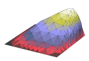
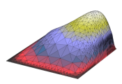
Figure 1. Terminal solution iterates from Example 5.1. Left: solution iterate with $\gamma_{10}=5$ on level 10 with 237 dof. Center: solution iterate with $\gamma_{10}=3$ on level 20 with 1332 dof. Right: solution iterate with $\gamma_{10}=1$ on level 30 with 9613 dof.

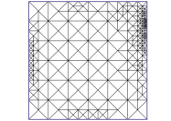
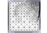
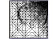
Figure 2. Adpative meshes from Example 5.1. Left: mesh on adaptive level 10 with 237 dof. Center: mesh on adaptive level 20 with 1332 dof. Right: mesh on adaptive level 30 with 9613 dof.

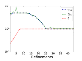
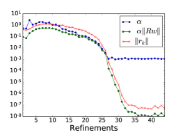
Figure 3. Left: regularization parameters $\gamma_{10}$, $\gamma_{01}$ and $\delta$. Right: regularization parameter $\alpha$, norm of regularization $\alpha\lVert{R{\tt w}}\rVert$, and the norm of the terminal residual $\lVert{r_{k}}\rVert,$ for Example 5.1, with nonlinear iterations running to tolerance ${\tt tol}=10^{-7}$.

Figure 1 shows snapshots of the computed iterates on refinements $10,20$ and $30$, with respectively $237,1332$ and $9313,$ degrees of freedom (dof), illustrating the progress from the preasymptotic into the asymptotic regimes. Figure 2 shows the corresponding adaptive meshes. The solution plots and meshes illustrate how the mesh is refined for both the boundary layer on either side of the origin; and, for the steep gradients in the diffusion coefficient. In this anisotropic case, the gradients are orders of magnitude steeper in the $x$- direction than the $y$- direction. In particular, $\kappa_{11}^{\prime}$ has a Lipschitz constant of approximately $2500$, while $\kappa_{22}^{\prime}$ has a Lipschitz constant of approximately $25$. It is observed that the meshes refine more in the vicinity of the steeper gradients; and, the mesh partition remains relatively coarse over large areas of the domain.

Figure 3 shows the terminal value of the regularization parameters $\gamma_{10}$, $\gamma_{01}$, $\delta$ and $\alpha$, on each level. For this example the plot on the left shows the scaling parameter $\delta\rightarrow 1$, rapidly, indicating accuracy of the Jacobian terms on the coarse mesh. The numerical dissipation parameter $\gamma_{10}$ hovers at its maximum value for the first sequence of updates, then decays steadily to one, as the updates converge to within tolerance given in (4.11) of Corollary 4.4. Decrease of $\gamma_{10}$ as in Lemma 4.3 is not relevant as for $\gamma_{\text{MAX}}=5$ and $q=0.865$ in this example, $\gamma_{\text{MONO}}$ given by (4.7) yields $\gamma_{\text{MONO}}<1$. The Picard-like regularization $\gamma_{01}$, shows a few spikes above it’s baseline level close to $\gamma_{10}$, and indeed remains active into the asymptotic regime, showing that the additional numerical diffusion maintains some cancellation properties against the linearization error. It was also observed numerically if this parameter were suppressed, that is $\sigma_{01}=0$ meaning $\gamma_{01}=\gamma_{10}$, the iterates tended to diverge after level 30.

The plot on the right side of Figure 3 shows the terminal value of the Tikhonov-like parameter $\alpha$ together with the norm of the scaled regularization term $\alpha\lVert{R{\tt w}^{n}}\rVert$, and terminal residual $\lVert{r_{k}}\rVert$ on each refinement level $k$. Here it is seen that due to the scaling of $\alpha$ by $\gamma_{10}/\lVert{R{\tt w}^{n}}\rVert$, the parameter $\alpha$ does not go to zero, however the definition (4.18) keeps the level of contributed regularization below the norm of the residual. Indeed, the plot of $\alpha$ diverges from the plot of $\alpha\lVert{R{\tt w}^{n}}\rVert$ as $\gamma\rightarrow 1$ and $\lVert{R{\tt w}^{n}}\rVert$ decreases into the asymptotic regime. It is remarked however, that the initial $\alpha_{k}^{0}=\lVert{r_{k}^{0}}\rVert$ on each refinement, then $\alpha$ decreases with the residual over each iteration. Without maintaining this low level of regularization into the asymptotic regime, the iterations were again observed to diverge.

The second example illustrates the updated regularization parameters on the model problem shown in previous work by the author [25, 26, 27]. In contrast to Example 5.1, here the parameters $\gamma_{10}$ and $\delta$ play a dominant role in the regularization, while $\sigma_{01}$ and $\alpha$ are less significant into the asymptotic regime.

Example 5.2 (Diffusion with thin layers).

Consider the quasilinear diffusion equation on $\Omega=(0,1)\times(0,1)$

$$-{\operatorname{div}}(\kappa(u)\nabla u)=f(x,y)\text{ in }\Omega,~{}u=0~{}\text{ on }~{}\partial\Omega,$$ (5.7)

with

$$\kappa(u) =k+\frac{1}{\varepsilon+(u-a)^{2}},$$ (5.8)

with the parameters $a=1/2$, $\varepsilon=10^{-5}$, and $k=1$. The source function $f$ is chosen so the exact solution $u(x,y)=\sin(\pi x)\sin(\pi y)$. This problem, featuring a bounded second derivative and high regularity of the solution, fits into both problem classes mentioned in Remark 1.3.

The initial regularization parameter $\gamma_{10}$ is set as $\gamma_{\text{MAX}}=(\sqrt{3}/2)\varepsilon^{-1/2}$, the approximate ratio of $\kappa^{\prime}(\bar{s})/\kappa(\bar{s})$, where $\bar{s}=\text{argmax\,}(\kappa^{\prime}(s))$. The regularization function $\phi(w,v)=(\nabla w,\nabla v)$, the standard Laplacian preconditioner.

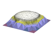
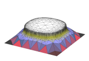
Figure 4. Terminal solution iterates from Example 5.2. Left: solution iterate with $\gamma_{10}=11$ on level 25 with 1511 dof. Center: solution iterate with $\gamma_{10}=5$ on level 30 with 3062 dof. Right: solution iterate with $\gamma_{10}=1$ on level 40 with 21678 dof.

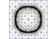
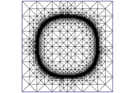
Figure 5. Adpative meshes from Example 5.2. Left: mesh on adaptive level 25 with 1511 dof. Center: mesh on adaptive level 30 with 3062 dof. Right: mesh on adaptive level 40 with 21768 dof.

Figure 4 shows snapshots of the solution progression through the preasymptotic and into the asymptotic regime. The snapshot on the left, from level 25 with 1511 dof, and the snapshot in the center, from level 30, with 3062 dof, show the effect of $\delta\ll 1$: the source function is scaled down so the solution iterates are held beneath the strong diffusion layer at $u=1/2$, until the diffusion in the vicinity of the ultimately thin layer is sufficiently resolved. Then, as $\delta\rightarrow 1$, the full strength source pushes the solution iterates through the diffusion layer, resulting in the asymptotic iterate on the right of Figure 4, on level 40 with 21678 dof. The corresponding meshes in Figure 5 illustrate the mesh refinement focused in the vicinity of the steep gradients of the diffusion layer.

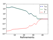
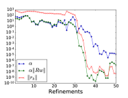
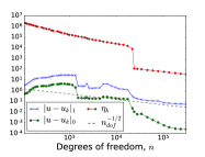
Figure 6. Left: regularization parameters $\gamma_{10}$, $\gamma_{01}$ and $\delta$. Center: regularization parameter $\alpha$, the norm of the regularization $\alpha\lVert{R{\tt w}}\rVert$, and the norm of the terminal residual $\lVert{r_{k}}\rVert$. Right: $H^{1}$ error, $|u-u_{k}|_{1}$; $L_{2}$ error, $|u-u_{k}|_{0}$; and, error estimator $\eta_{k}$, against $n_{dof}^{-1/2}$, degrees of freedom, for Example 5.2, with nonlinear iterations running to tolerance ${\tt tol}=10^{-7}$.

The first two plots of Figure 6 shows the terminal values of each regularization parameter $\gamma_{10},\gamma_{01},$ $\delta$ and $\alpha$ on each refinement level. On the left, it is seen as $\gamma_{10}$ progresses from $\gamma_{\text{MAX}}$ of approximately 250 down to 1, the initial relationship $\delta=1/\gamma_{10}$ is roughly maintained. From this plot it is also apparent that the regularization parameter $\sigma_{01}$ plays only a minor role in the stabilization of the Jacobian, and $\gamma_{01}\approx\gamma_{10}$ throughout the simulation.

Figure 6 in the center, shows the terminal value of $\alpha$, which scales the Tikhonov-like regularization term, plotted together with the full norm of the Tikhonov-like term $\alpha\lVert{R{\tt w}^{n}}\rVert$, and the final residual on each iteration $\lVert{r_{k}}\rVert$. The effect of scaling $\alpha$ against the norm of $R{\tt w}^{n}$ is seen to be small in the preasymptotic regime where $\lVert{R{\tt w}^{n}}\rVert={\mathcal{O}}(1)$. This scaling is however of increasing importance into the asymptotic phase, to reduce this regularization to the order of the residual norm, for fast convergence.

After refinement level 28, as $\gamma_{10}<\gamma_{\text{MONO}}=96$, given by Lemma 4.3, the residual decrease exit criteria, (4.31)-(4.32) of Condition (2), Critia 4.5, is enforced, resulting in the rapid decrease of the residual over the next several refinements, seen in Figure 6 on the right. Finally, it is noted in the plot on the right of Figure 6, that upon entering the asymptotic regime with the residual solving to tolerance at each iteration, the $H^{1}$ error reduces at the rate $n_{dof}^{-1/2}$, the expected rate for the corresponding linear problem.

6. Conclusion

This paper describes a framework for pseudo-time regularization, applied to a generally nonmonotone class of quasilinear partial differential equations. The regularization, which is designed to exploit the quasilinear structure of the equation, is first derived from the discrete problem at the PDE level. The regularized linear algebraic system is then specified under inexact assembly. The residual representation of the assembled system then reveals the errors induced from regularization, linearization and floating-point arithmetic; and, allows insight into how regularization can control the linearization error. An updated set of regularization parameters is presented, then applied to an adaptive algorithm to approximate the solution of quasilinear PDE of nonmonotone type. The method is demonstrated on two problems, the first of which features an anisotropic diffusion coefficient that is not twice differentiable. The second demonstrates recovering a known solution from a model problem with a thin diffusion layer. The results suggest theoretical convergence of the error without a sufficiently-fine mesh condition or a second derivative on the solution-dependent diffusion coefficient should be possible.

7. Acknowledgments

The author would like to thank William Rundell and Yunrong Zhu for numerous interesting discussions on the topics addressed here, and for input on a draft of this manuscript.

References

- [1] S. Balay, S. Abhyankar, M. F. Adams, J. Brown, P. Brune, K. Buschelman, L. Dalcin, V. Eijkhout, W. D. Gropp, D. Kaushik, M. G. Knepley, L. C. McInnes, K. Rupp, B. F. Smith, S. Zampini, H. Zhang, and H. Zhang. PETSc users manual. Technical Report ANL-95/11 - Revision 3.7, Argonne National Laboratory, 2016.
- [2] R. Bank and D. Rose. Parameter selection for Newton-like methods applicable to nonlinear partial differential equations. SIAM J. Numer. Anal., 17(6):806–822, 1980.
- [3] L. Belenki, L. Diening, and C. Kreuzer. Optimality of an adaptive finite element method for the p-Laplacian equation. IMA J. Numer. Anal., 32(2):484–510, 2012.
- [4] C. Bi and V. Ginting. A posteriori error estimates of discontinuous Galerkin method for nonmonotone quasi-linear elliptic problems. J. Sci. Comput., 55(3):659–687, 2013.
- [5] G. Caloz and J. Rappaz. Numerical analysis for nonlinear and bifurcation problems. In Techniques of Scientific Computing (Part 2), volume 5 of Handbook of Numerical Analysis, pages 487 – 637. Elsevier, 1997.
- [6] P. G. Ciarlet. Finite Element Method for Elliptic Problems. Society for Industrial and Applied Mathematics, Philadelphia, PA, USA, 2002.
- [7] T. S. Coffey, C. T. Kelley, and D. E. Keyes. Pseudo-transient continuation and differential-algebraic equations. SIAM J. Sci. Comput., 25:553–569, 2003.
- [8] J. Crank. The mathematics of diffusion. Clarendon Press, Oxford, 1975.
- [9] P. Deuflhard. Newton Methods for Nonlinear Problems: Affine Invariance and Adaptive Algorithms. Springer Publishing Company, Incorporated, 2011.
- [10] P. Deuflhard and F. A. Potra. Asymptotic mesh independence of Newton-Galerkin methods via a refined Mysovskii theorem. SIAM J. Numer. Anal., 29(5):1395–1412, 10 1992.
- [11] J. Douglas and T. Dupont. A Galerkin method for a nonlinear Dirichlet problem. Mathematics of Computation, (131):689, 1975.
- [12] J. Douglas, T. Dupont, and J. Serrin. Uniqueness and comparison theorems for nonlinear elliptic equations in divergence form. Arch. for Ration. Mech. Anal., 42(3):157, 1971.
- [13] H. Engl, M. Hanke, and A. Neubauer. Regularization of Inverse Problems. Mathematics and Its Applications. Springer, 1996.
- [14] A. Ern and M. Vohralík. Adaptive inexact Newton methods with a posteriori stopping criteria for nonlinear diffusion PDEs. SIAM J. Sci. Comput., 35(4):A1761–A1791, 2013.
- [15] M. W. Farthing, C. E. Kees, T. S. Coffey, C. Kelley, and C. T. Miller. Efficient steady-state solution techniques for variably saturated groundwater flow. Advances in Water Resources, 26:833 – 849, 2003.
- [16] O. Ferreira. Local convergence of newton’s method under majorant condition. J. of Comput. Appl. Math., 235:1515 – 1522, 2011.
- [17] E. M. Garau, P. Morin, and C. Zuppa. Convergence of an adaptive Kačanov FEM for quasi-linear problems. Appl. Numer. Math., 61(4):512 – 529, 2011.
- [18] T. Gudi and A. K. Pani. Discontinuous Galerkin methods for quasi-linear elliptic problems of nonmonotone type. SIAM J. Numer. Anal., (1):163, 2007.
- [19] I. Hlavác̆ek, M. Kr̆íz̆ek, and J. Malý. On Galerkin approximations of a quasilinear nonpotential elliptic problem of a nonmonotone type. J. Math. Anal. Appl., 184(1):168, 1994.
- [20] M. Holst, N. Baker, and F. Wang. Adaptive multilevel finite element solution of the Poisson-Boltzmann equation I. Algorithms and examples. J. Comput. Chem, 21(15):1319, 2000.
- [21] M. Holst, G. Tsogtgerel, and Y. Zhu. Local and global convergence of adaptive methods for nonlinear partial differential equations, 2008.
- [22] C. T. Kelley and D. Keyes. Convergence analysis of pseudo-transient continuation. SIAM J. Numer. Anal., 35(2):508–523, 1998.
- [23] A. Logg, K.-A. Mardal, G. N. Wells, et al. Automated Solution of Differential Equations by the Finite Element Method. Springer, 2012.
- [24] N. M. Newmark. A method of computation for structural dynamics. J. Eng. Mech.-ASCE, 85(EM3):67–94, 1959.
- [25] S. Pollock. A regularized Newton-like method for nonlinear PDE. Numer. Func. Anal. Opt., 36(11):1493–1511, 2015.
- [26] S. Pollock. An improved method for solving quasilinear convection diffusion problems. SIAM J. Sci. Comput., 38(2):A1121–A1145, 2016.
- [27] S. Pollock. Stabilized and inexact adaptive methods for capturing internal layers in quasilinear PDE. J. Comput. Appl. Math, pages 243–262, 2016. DOI: 10.1016/j.cam.2016.06.011.
- [28] R. Stevenson. Optimality of a standard adaptive finite element method. Found. Comput. Math., 7(2):245–269, 2007.
- [29] X. Zhang. Uniqueness of weak solution for nonlinear elliptic equations in divergence form. Internat. J. Math. Math. Sci., (5):313, 2000.