The anatomy of the Orion B Giant Molecular Cloud:
A local template for studies of nearby galaxies

Abstract

Context. Molecular lines and line ratios are commonly used to infer properties of extra-galactic star forming regions. The new generation of millimeter receivers turns every observation nearly into a line survey. To fully exploit this technical advance in extra-galactic studies requires detailed bench-marking of available line diagnostics.

Aims. We aim to develop the Orion B Giant Molecular Cloud (GMC) as a local template for interpreting extra-galactic molecular line observations.

Methods. We use the wide-band receiver at the IRAM-30m to spatially and spectrally resolve the Orion B GMC. The observations cover almost 1 square degree at $26^{\prime\prime}$ resolution with a bandwidth of 32$\mathrm{\,GHz}$ from 84 to 116$\mathrm{\,GHz}$ in only two tunings. Among the mapped spectral lines are the $\mathrm{{}^{12}CO}$, $\mathrm{{}^{13}CO}$, $\mathrm{C^{18}O}$, $\mathrm{C^{17}O}$, $\mathrm{HCN}$, $\mathrm{HNC}$, $\mathrm{{}^{12}CN}$, $\mathrm{C_{2}H}$, $\mathrm{HCO^{+}}$, $\mathrm{N_{2}H^{+}}$ $\mathrm{(1-0)}$, and $\mathrm{{}^{12}CS}$, $\mathrm{{}^{32}SO}$, $\mathrm{SiO}$, $\mathrm{c-C_{3}H_{2}}$, $\mathrm{CH_{3}OH}$ $\mathrm{(2-1)}$ transitions.

Results. We introduce the molecular anatomy of the Orion B GMC, including relations between line intensities and gas column density or far-UV radiation fields, and correlations between selected line and line ratios. We also obtain a dust-traced gas mass that is less than about one third the CO-traced mass, using the standard $X_{\mathrm{CO}}$ conversion factor. The presence of overluminous CO can be traced back to the dependence of the CO intensity on UV illumination. As a matter of fact, while most lines show some dependence on the UV radiation field, CN and $\mathrm{C_{2}H}$ are the most sensitive. Moreover dense cloud cores are almost exclusively traced by $\mathrm{N_{2}H^{+}}$. Other traditional high density tracers, such as $\mathrm{HCN}$$\mathrm{(1-0)}$, are also easily detected in extended translucent regions at a typical density of $\sim 500\,\mathrm{H_{2}}\mathrm{\,cm^{-3}}$. In general, we find no straightforward relation between line critical density and the fraction of the line luminosity coming from dense gas regions.

Conclusions. Our initial findings demonstrate that the relations between line (ratio) intensities and environment in GMCs are more complicated than often assumed. Sensitivity (i.e., the molecular column density), excitation, and above all chemistry contribute to the observed line intensity distributions, and they must be considered together when developing the next generation of extra-galactic molecular line diagnostics of mass, density, temperature and radiation field.

Table 1: Properties of the stars exciting the H ii regions in the observed field of view.

H ii region	Star	Type	$\alpha,\delta$ (J2000)	$(\delta x,\delta y)$	Parallax	Distance	$V_{\mathrm{LSR}}$
				$(^{\prime\prime},^{\prime\prime})$	mas	pc	$\mathrm{\,km\,s^{-1}}$
IC 434	$\sigma$Ori	O9.5V B	$\mathrm{05^{h}38^{m}44.779^{s},-02^{\circ}36^{{}^{\prime}}00.12^{{}^{\prime\prime}}}$	$(-33.35,00.07)$	$2.5806\pm 0.0088^{(1)}$	$387.5\pm 1.3$(1)	$15.0\pm 1.6$
IC 435	HD 38087	B5V D	$\mathrm{05^{h}43^{m}00.573^{s},-02^{\circ}18^{{}^{\prime}}45.38^{{}^{\prime\prime}}}$	$(+32.87,01.33)$	$5.90\pm 1.29^{(2)}$	$169\pm 37$(2)	$18.1\pm 4.5$
NGC 2023	HD 37903	B1.5V C	$\mathrm{05^{h}41^{m}38.388^{s},-02^{\circ}15^{{}^{\prime}}32.48^{{}^{\prime\prime}}}$	$(+13.72,09.42)$	$2.776\pm 0.271^{(3)}$	$362\pm 35$(3)	$-7.7\pm 2$
NGC 2024	IRS2b	O8V-B2V	$\mathrm{05^{h}41^{m}45.50^{s},-01^{\circ}54^{{}^{\prime}}28.7^{{}^{\prime\prime}}}$	$(+20.54,29.43)$	—	$415$(4)	—
	Alnitak	O9.7Ib+B0III C	$\mathrm{05^{h}40^{m}45.527^{s},-01^{\circ}56^{{}^{\prime}}33.26^{{}^{\prime\prime}}}$	$(+05.49,31.04)$	$3.4\pm 0.2^{(5)}$	$294\pm 21$(5)	$3.7\pm 1.3$

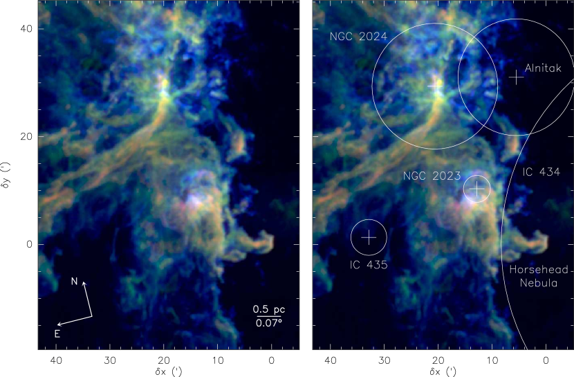
Figure 1: Composite image of the $\mathrm{{}^{12}CO}$ (blue), $\mathrm{{}^{13}CO}$ (green), $\mathrm{C^{18}O}$ (red) $\mathrm{(1-0)}$ peak-intensity main-beam temperature. The circles show the typical extensions of the H ii regions and the crosses show the position of the associated exciting stars (see Table 1). The $\sigma$-Ori star that excites the IC 434 H ii region is located 0.5^∘ East from the Horsehead nebula.

1 Introduction

The star formation process from interstellar gas raises many outstanding questions. For instance, what is the relative role of micro-physics and galactic environment on the star formation efficiency? More precisely, what is the role of magnetic field, gravity, turbulence (see e.g., Hennebelle & Chabrier, 2011; Hennebelle, 2013), on one hand, and of external pressure, position in galactic arm/interarms, streaming motions (e.g., Meidt et al., 2013; Hughes et al., 2013), on the other hand? How does feedback from H ii region expansions and supernovae limit the star formation efficiency (Kim et al., 2013)? What are the key dynamical parameters controlling star formation: Mach number, virial parameter, amount of energy in solenoidal/compressive modes of the turbulence (Federrath & Klessen, 2012, 2013)? What is the amount of CO-dark molecular gas and does it bias the global estimation of the mass of the molecular reservoir at cloud scales (Wolfire et al., 2010; Liszt & Pety, 2012)? What is the amount of diffuse $(\sim 100-500\mathrm{\,cm^{-3}},80\mathrm{\,K})$ vs. dense $(\sim 10^{4}\mathrm{\,cm^{-3}},10\mathrm{\,K})$ gas in a GMC? In other words, what is the fraction of star-forming dense gas (Lada et al., 2010, 2012, 2013)?

All these questions also arise in extra-galactic studies with the additional difficulty that GMCs are unresolved at the typically achieved angular resolution ($1^{\prime\prime}$ corresponds to 15$\mathrm{\,pc}$ for a 3$\mathrm{\,Mpc}$ distant galaxy). It is therefore crucial to first understand how the average spectra of molecular lines relate to actual physical properties when the line emission is spatially resolved. By mapping a significant fraction of a GMC at a spatial resolution of $\sim 50\mathrm{\,mpc}$ and a spectral resolution of $0.6\mathrm{\,km\,s^{-1}}$, we address some of the following issues: What linear resolution must be achieved on a GMC to correctly derive its global properties including star formation rate and efficiency (Leroy et al., 2016)? For instance, are usual extra-galactic line tracers of the various molecular cloud density regimes reliable (Bigiel et al., 2016)? Do we get a more accurate estimate of the mass by resolving the emission? More generally, can we derive empirical laws that link tracer properties averaged over a GMC to its internal star forming activity?

With the advent of wide-bandwidth receivers associated to high resolution spectrometers, any observation now simultaneously delivers emission from many different tracers. Moreover, the increased sensitivity makes it possible to cover large fields of view. The possibility to map many different lines in many different environments allows us to start answering the questions presented above. The essence of the ORION-B (Outstanding Radio Imaging of OrioN B, PI: J. Pety) project is to recast the science questions of star formation in a statistical way. Wide-field hyper-spectral mapping of Orion B is used to obtain an accurate 3D description of the molecular structure in a Giant Molecular Cloud, a key for defining chemical probes of the star formation activity in more distant Galactic and extragalactic sources.

About thirty 3$\mathrm{\,mm}$ lines are detected in only two frequency tunings with the same sensitive radio single-dish telescope at a typical resolution of $26^{\prime\prime}$ over almost 1 square degree. The field of view ($5.6\times 7.5\mathrm{\,pc}$) would fall in a single resolution element of a map of the Orion B molecular cloud observed at 3$\mathrm{\,mm}$ with a telescope of similar diameter as the IRAM-30m from the Small or Large Magellanic Clouds. The spectra averaged over the field of view would then represent the spectra of Orion B as seen by an alien from the Magellanic Clouds. Conversely, our imaging experiment allows us to reveal the detailed anatomy of a molecular emission that is usually hidden behind these mean spectra in nearby galaxy studies. The south-western edge of the Orion B molecular cloud (a.k.a. Barnard 33 or Lynds 1630) represents an ideal laboratory for this kind of study. It forms both low-mass and massive stars. It contains regions of triggered or spontaneous star formation, photon-dominated regions and UV-shielded cold gas, all in a single source.

In companion papers, Gratier et al. (subm.) study a Principal Component Analysis of the same dataset to understand the main correlations that exist between the different lines. Orkisz et al. (subm.) quantify the fractions of turbulent energy that are associated to the solenoidal/compressive modes, and they relate these values to the star formation efficiency in Orion B. In this paper, we present the observational results of the ORION-B project, focusing on the mean properties of this GMC and evaluate the diagnostic power of commonly used line tracers and ratios.

We present the targeted field of view, as well as the observations and data reduction process in Section 2. Typical properties, such as UV-illumination, mean line profiles, CO-traced, dust-traced and virial masses, are computed in Section 3. In Section 4, we investigate the fraction of flux arising in different gas regimes for each line. In Section 5.1, we compare the visual extinction map with the line integrated intensities and compute the luminosity per proton of the different line tracers. The properties of various line ratios are discussed in Section 6. A discussion is presented in Section 7, focusing on possible biases introduced by the characteristics of the observed field of view, and whether the $\mathrm{HCO^{+}}$, $\mathrm{HCN}$, and $\mathrm{HNC}$ $\mathrm{(1-0)}$ lines are good tracers of dense gas. We end the discussion by comparing the observed line ratios in Orion B with extra-galactic observation results. Section 8 summarizes the results and concludes the paper.

2 The Orion B Giant Molecular Cloud

Table 2: Typical properties of the South-Western edge of Orion B.

Parameter	Value	Notes
Distance	$400\mathrm{\,pc}$	$1^{\prime\prime}=2\mathrm{\,mpc}$
Systemic velocity	$10.5\mathrm{\,km\,s^{-1}}$	LSR, radio convention
Projection center	$\mathrm{05^{h}40^{m}54.270^{s},-02^{\circ}28^{{}^{\prime}}00.00^{{}^{\prime\prime}}}$	$\alpha,\delta$(J2000), mane of the Horsehead
Offset range & Field of view	$[-5.2^{\prime},+43.3^{\prime}]\times[-19.5^{\prime},45.3^{\prime}]$	$49^{\prime}\times 65^{\prime}$ or $5.6\times 7.5\mathrm{\,pc}$
$W^{\mathrm{min}}_{\mathrm{CO}}-W^{\mathrm{mean}}_{\mathrm{CO}}-W^{\mathrm{max}}_{\mathrm{CO}}$	$0-61-288\mathrm{\,K\,km\,s^{-1}}$	in $[-2,+18]\mathrm{\,km\,s^{-1}}{}$
$A_{\mathrm{V}}^{\mathrm{min}}-A_{\mathrm{V}}^{\mathrm{mean}}-A_{\mathrm{V}}^{\mathrm{max}}$	$0.7-4.7-222\mathrm{\,mag}$	$A_{\mathrm{K}}/A_{\mathrm{V}}^{\mathrm{}}=0.13$
$T_{\mathrm{d}}^{\mathrm{min}}-T_{\mathrm{d}}^{\mathrm{mean}}-T_{\mathrm{d}}^{\mathrm{max}}$	$16-26-99\mathrm{\,K}$
$G_{0}^{\mathrm{min}}-G_{0}^{\mathrm{mean}}-G_{0}^{\mathrm{max}}$	$4-45-36000$	Inter-Stellar Radiation Field (Habing, 1968)
CO-traced mass	$11000\mathrm{\,M_{\odot}}$	Standard $X_{\mathrm{CO}}$ & Helium dealt with
Dust-traced mass	$3900\mathrm{\,M_{\odot}}$	Standard $N_{\mathrm{H}}$/$A_{\mathrm{V}}^{\mathrm{}}$ & H i gas negligible
Virial traced mass	Between $6200$ and $9500\mathrm{\,M_{\odot}}$	Depending on the assumed density radial profile
Imaged surface	$43\mathrm{\,pc}^{2}$	$=S$
Typical volume	$280\mathrm{\,pc}^{3}$	$=S^{3/2}$
CO-traced mean column density	$260\mathrm{\,M_{\odot}}\mathrm{\,pc}^{-2}$ — $12\times 10^{21}\mathrm{H_{2}}{}\mathrm{\,cm^{-2}}$	Standard $X_{\mathrm{CO}}$ & Helium dealt with
Dust-traced mean column density	$92\mathrm{\,M_{\odot}}\mathrm{\,pc}^{-2}$ — $4\times 10^{21}\mathrm{H_{2}}{}\mathrm{\,cm^{-2}}$	Standard $N_{\mathrm{H}}$/$A_{\mathrm{V}}^{\mathrm{}}$ & H i gas negligible
CO-traced mean volume density	$40\mathrm{\,M_{\odot}}\mathrm{\,pc}^{-3}$ — $590\mathrm{H_{2}}{}\mathrm{\,cm^{-3}}$	Standard $X_{\mathrm{CO}}$ & Helium dealt with
Dust-traced mean volume density	$14\mathrm{\,M_{\odot}}\mathrm{\,pc}^{-3}$ — $210\mathrm{H_{2}}{}\mathrm{\,cm^{-3}}$	Standard $N_{\mathrm{H}}$/$A_{\mathrm{V}}^{\mathrm{}}$ & H i gas negligible

2.1 Targeted field of view

Figure 1 displays a composite image of the $\mathrm{{}^{12}CO}$ (blue), $\mathrm{{}^{13}CO}$ (green), $\mathrm{C^{18}O}$ (red) $\mathrm{(1-0)}$ peak-intensity main-beam temperatures. It shows the south-western edge of the Orion B molecular cloud. This region samples the interaction of the molecular cloud with at least 4 H ii regions. First, $σ$Ori is an O9.5V star that illuminates the western edge of the Orion B cloud. It creates the IC 434 nebula from which the Horsehead pillar emerges. Second, NGC 2023 and NGC 2024 are two younger H ii regions embedded in the Orion B molecular cloud, powered by B1.5V (HD 37903) or late O, early B (IRS2b) stars, respectively (Bik et al., 2003). NGC 2024 covers 20 arcminutes at the northern edge of the mapped field of view, while NGC 2023 is situated approximately halfway between IRS2b and the Horsehead. The B5V HD 38087 star creates the IC 435 nebula at the south-eastern edge of the field of view. Finally, one of the 3 Orion Belt stars, the O9.71b star Alnitak (a.k.a. $\zeta$Ori), falls in the observed field of view. Table 1 lists the characteristics of these exciting stars. To guide the eye, we overlaid on the right panel of Fig. 1 crosses at the position of the main exciting stars, and circles at the approximate boundaries of the different H ii regions. These visual markers will be used throughout the paper.

2.2 IRAM-30m observations

The observations were taken with the IRAM-30m telescope in four observing runs: August 2013, December 2013, August 2014, and November 2014 during 133 hours in total (telescope time) under average summer weather (6$\mathrm{\,mm}$ median water vapor) and good winter weather (3$\mathrm{\,mm}$ median water vapor). During all these runs, we observed with a combination of the 3$\mathrm{\,mm}$ sideband separated EMIR receivers and the Fourier transform spectrometers, which yields a total bandwidth of $\sim 32\mathrm{\,GHz}$ per tuning (i.e., $\sim 8\mathrm{\,GHz}$ per sideband and per polarization) at a channel spacing of 195$\mathrm{\,kHz}$ or $0.5-0.7\mathrm{\,km\,s^{-1}}$. The two tuned frequencies were 102.519$\mathrm{\,GHz}$ and 110.000$\mathrm{\,GHz}$ at the 6.25$\mathrm{\,MHz}$ intermediate frequency of the upper sideband, resulting in local oscillator frequencies of 96.269 and 103.750$\mathrm{\,GHz}$, respectively. This allowed us to observe nearly the entire 3$\mathrm{\,mm}$ band from 84.5 to 115.5$\mathrm{\,GHz}$.

We used the on-the-fly scanning strategy with a dump time of 0.25 seconds and a scanning speed of $17^{\prime\prime}/$s to ensure a sampling of 5 dumps per beam along the scanning direction at the $21.2^{\prime\prime}$ resolution reached at the highest observed frequency, i.e., 116$\mathrm{\,GHz}$. We covered the full field of view ($\sim 0.9$ square degrees) with $\sim 103$ tiles of $\sim 110^{\prime\prime}\times 1000^{\prime\prime}$ size. The rectangular tiles had a position angle of $14^{\circ}$ in the Equatorial J2000 frame to adapt the mapping strategy to the global morphology of the Western edge of the Orion B molecular cloud. These tiles were covered with rasters along their long axis (almost the Dec direction). The separation between two successive rasters was $\lambda/2D=8.46^{\prime\prime}$ to ensure Nyquist sampling perpendicular to the scanning direction. The scanning direction was reversed at the end of each line (zigzag mode). This implied a tongue and groove shape at the bottom and top part of each tile. We thus overlapped by $30^{\prime\prime}$ the top and bottom edges of the tiles to ensure a correct sampling. On the other hand, the left and right edges of the tiles were adjusted to avoid any overlap, i.e., to maximize the overall scanning speed. The field of view was covered only once by the telescope, except for the tiles observed in the worst conditions (low elevation and/or bad weather) that were repeated once.

The calibration parameters (including the system temperature) were measured every 15 minutes. The pointing was checked every two hours and the focus every 4 hours. Following Mangum et al. (2007) and Pety et al. (2009), we used the optimum position switching strategy. A common off reference position was observed during 11 seconds every 59 seconds with the following repeated sequence OFF-OTF-OTF-OFF. No reference position completely devoid of $\mathrm{{}^{12}CO}$ $\mathrm{(1-0)}$ emission could be localized in the close neighborhood of the Orion B western edge. As this reference position is subtracted to every OTF spectrum in order to remove the common atmospheric contribution, the presence of signal in the reference position results in a spurious negative contribution to the signal everywhere in the final cube. Searching for a reference position farther away in the hope that it is devoid of signal would degrade the quality of the baseline because the atmospheric contribution would vary from the OTF spectra to the reference position. We thus tested several nearby potential reference positions using the frequency-switched observing mode that does not require a reference position. This is possible because the observed lines have narrow linewidth. We then selected the nearest position that has the minimum line integrated emission in $\mathrm{{}^{12}CO}$ $\mathrm{(1-0)}$. Offsets of this position are $(-500^{\prime\prime},-500^{\prime\prime})$ with respect to the projection center given in Table 2. The $\mathrm{{}^{12}CO}$, and $\mathrm{{}^{13}CO}$ $\mathrm{(1-0)}$ peak intensities at this position are $\sim 1$ and 0.05$\mathrm{\,K}$, respectively. The correction of the negative contribution from the reference position to the final cube requires a good observation of the reference position. We therefore observed this reference position using the frequency-switched observing mode in both tunings, a few minutes per observing session.

2.3 IRAM-30m data reduction

Data reduction was carried out using the GILDAS/CLASS software. The data were first calibrated to the $T_{\mathrm{A}}^{*}$ scale using the chopper-wheel method (Penzias & Burrus, 1973). The data were then converted to main-beam temperatures ($T_{\mathrm{mb}}$) using the forward and main-beam efficiencies ($F_{\mathrm{eff}}$ and $B_{\mathrm{eff}}$) listed in Table 12. The $B_{\mathrm{eff}}$ values are derived from the Ruze’s formula

$$B_{\mathrm{eff}}{}(\lambda)=B_{\mathrm{eff}}^{0}\,\exp\left\{-\left(\frac{4\pi\,\sigma}{\lambda}\right)^{2}\right\}$$ (1)

$$\mbox{with}\quad B_{\mathrm{eff}}^{0}=0.863,\quad\mbox{and}\quad\sigma=65.6\mathrm{\,\mu m},$$ (2)

where $\lambda$ presents the wavelength dependence. The resulting amplitude accuracy is $\sim 10\%$. A 12 to 20$\mathrm{\,MHz}$-wide subset of the spectra was first extracted around each line rest frequency. We computed the observed noise level after subtracting a first order baseline from every spectrum, excluding the velocity range from 0 to 18$\mathrm{\,km\,s^{-1}}$ LSR, where the gas emits for all observed lines, except $\mathrm{{}^{12}CO}$ and $\mathrm{HCO^{+}}$ $\mathrm{(1-0)}$ for which the excluded velocity range was increased from -5 to 20$\mathrm{\,km\,s^{-1}}$ LSR. A systematic comparison of this noise value with the theoretical noise computed from the system temperature, the integration time, and the channel width, allowed us to filter out outlier spectra (typically 3% of the data).

To correct for the negative contribution from the reference position to the final cube, we first averaged all the observations of the reference position 1) to increase the signal-to-noise ratio of the measured profiles, and 2) to decrease the influence of potential calibration errors. Signal in the reference position was only detected for the $\mathrm{{}^{12}CO}$ and $\mathrm{{}^{13}CO}$ $\mathrm{(1-0)}$ lines. The correction was thus applied only for these two lines. The averaged spectra at these frequencies were fitted by a combination of Gaussians after baseline subtraction, in order to avoid adding supplementary noise in the final cube. This fit was then added to every on-the-fly spectrum.

The spectra were then gridded into a data cube through a convolution with a Gaussian kernel of $\mathrm{FWHM}\sim 1/3$ of the IRAM-30m telescope beamwidth at the rest line frequency. To facilitate comparison of the different line cubes, we used the same spatial (pixels of $9^{\prime\prime}$ size) and spectral (80 channels spaced by 0.5$\mathrm{\,km\,s^{-1}}$) grid. The position-position-velocity cubes were finally smoothed at the common angular resolution of $31^{\prime\prime}$ to avoid resolution effects.

2.4 Map of visual extinction and dust temperature from Herschel and Planck data

In this paper, we will observationally check the potential of line intensities and of ratios of line intensities to characterize physical properties of the emitting gas. Ancillary data are thus needed to deliver independent estimates of these physical properties. We will use recent dust continuum observations to provide estimates of the column density of material and of the far UV illumination.

After combining the Herschel Gould Belt Survey (André et al., 2010; Schneider et al., 2013) and Planck observations (Planck Collaboration et al., 2011a) in the direction of Orion B, Lombardi et al. (2014) fitted the spectral energy distribution to yield a map of dust temperature and a map of dust opacity at 850$\mathrm{\,\mu m}$ ($\tau_{\mathrm{850}}$). Hollenbach et al. (1991) indicates that the equilibrium dust temperature at the slab surface of a 1D Photo-Dissociation Region (PDR) is linked to the incident far UV field, $G_{0}^{\mathrm{}}$ at $A_{\mathrm{V}}^{\mathrm{}}=0$, through

$$T_{\mathrm{d}}^{\mathrm{}}=12.2\,G_{0}^{\mathrm{0.2}}\mathrm{\,K},$$ (3)

where the $G_{0}^{\mathrm{}}$ value is given in units of the local interstellar radiation field (ISRF, Habing, 1968). We will invert this equation to give an approximate value of the far UV illumination. This value is likely a lower limit to the actual $G_{0}^{\mathrm{}}$ in most of the mapped region. Indeed, it is the far UV field at the surface of the PDR, while there are embedded H ii regions in the field of view. However, Abergel et al. (2002) estimates a typical $G_{0}^{\mathrm{}}\sim 100$ for the western edge of L 1630, which is a large scale edge-on PDR. Using Eq. 3, this value is compatible with the typical dust temperature fitted towards this edge, i.e., about 30$\mathrm{\,K}$.

Lombardi et al. (2014) compared the obtained 850$\mathrm{\,\mu m}$ opacity map to an extinction map in the K band ($A_{\mathrm{K}}$) of the region. A linear fit of the scatter diagram of $A_{\mathrm{K}}$ and $\tau_{\mathrm{850}}$ give for Orion B $A_{\mathrm{K}}=3460\,\tau_{\mathrm{850}}$ (Lombardi et al. (2014) name this factor $\gamma$). They used a value of $A_{\mathrm{K}}/A_{\mathrm{V}}^{\mathrm{}}=0.112$ from Rieke & Lebofsky (1985). However, this value, including their estimated $R_{\mathrm{V}}^{\mathrm{}}\simeq 3.1$, is not based on observations towards Orion stars. Cardelli et al. (1989) measured the properties of dust absorption $E_{\mathrm{B-V}}$ and $R_{\mathrm{V}}^{\mathrm{}}$ towards two stars of our field of view. Using their parametrization, we yield $A_{\mathrm{K}}/A_{\mathrm{V}}^{\mathrm{}}=0.1254$ for $R_{\mathrm{V}}^{\mathrm{}}=4.11$ towards HD 37903, and $A_{\mathrm{K}}/A_{\mathrm{V}}^{\mathrm{}}=0.1335$ for $R_{\mathrm{V}}^{\mathrm{}}=5.30$ towards HD 38087. We here take an average of both values, $A_{\mathrm{K}}/A_{\mathrm{V}}^{\mathrm{}}=0.13$, i.e., a 20% larger value than Rieke & Lebofsky (1985). We therefore have

$$A_{\mathrm{V}}^{\mathrm{}}=2.7\times 10^{4}\,\tau_{\mathrm{850}}\mathrm{\,mag}.$$ (4)

The dust properties (both the temperature and visual extinction) are measured at an angular resolution of $36^{\prime\prime}$.

2.5 Noise properties, data size, percentage of signal channels, line integrated intensities

The median noise levels (computed on the cubes that have 0.5$\mathrm{\,km\,s^{-1}}$ channel spacing and $31^{\prime\prime}$ angular resolution) range from 100 to 180$\mathrm{\,mK}$ ($T_{\mathrm{mb}}$) depending of the observed frequency. Details can be found in Appendix A. The reduced data cube amounts to about 160 000 images of $325\times 435$ pixels or 84 GB of uncompressed data. It would make a movie of 1h50m at 24 images per second. However, about 99.5% of the channels show mostly noise because of the limited sensitivity of our observation. The 0.5% of the bandwidth where clear signal is detected includes the emission from low $J$ lines of CO, $\mathrm{HCO^{+}}$, HCN, HNC, CN, CS, SO, $\mathrm{C_{2}H}$, $\mathrm{c-C_{3}H_{2}}$, $\mathrm{N_{2}H^{+}}$, $\mathrm{CH_{3}OH}$, SiO, and some of their isotopologues, in particular, CO isotopologues (see Table 4 and Fig. 2).

Most of this paper will study the properties of the line integrated intensity defined as $W=\int T(v)\,dv$. To produce reliable spectral line maps, we used all the pixels matching two conditions: 1) its own signal-to-noise ratio is larger than 4, and 2) the signal-to-noise ratio of at least 25% of its neighbors are larger than 4. Residual striping may be seen along the vertical scanning direction in particular at low intensity on the images of line integrated intensities. Indeed, baselining corrects for the striping to first order. Hence residual striping is more visible for faint lines and/or lines for which the overlapping of the velocity and the hyperfine structures require the definition of wider baselining windows, e.g., for the $\mathrm{HCN}$ ground state transition. Finally, we used two different flavors of the integrated intensity. On one hand, we will use the line intensity integrated over the full line profiles when we aim at studying the gas properties along the full line of sight. This will happen, for instance, when we will compute the CO-traced mass in Section 3.4 and the correlations between the column density of material along the full line of sight and the line integrated intensity in Section 5. On the other hand, lines are detected over different velocity ranges. Using the same velocity range for all lines, e.g., $[-2,+18\mathrm{\,km\,s^{-1}}]$, will result in noisy integrated intensities for tracers that have the narrowest lines. In contrast, adapting the velocity range to each line could bias the results. We thus adopted a compromise for sections where we can restrict our investigations to the bulk of the gas: We computed the line integrated intensity over the velocity range where the core of the line can be found for each species and transition over the measured field of view. This velocity range is $[9,12\mathrm{\,km\,s^{-1}}]$.

3 Mean properties

Figure 2: Spatial distribution of the line integrated intensity for some of the detected lines in the 3mm band, plus the dust temperature (bottom left panel) and the visual extinction (top right corner). Continuum data comes from the publicly available SED fit done by Lombardi et al. (2014) on the Herschel Gould Belt Survey data (PI: P. André). The color scales are logarithmic to reveal the distribution of faint signal. Pixels with a signal-to-noise lower than 4 were blanked out. In addition to the circles and crosses that show the approximate boundaries of the H ii regions and the associated exciting stars, we overlaid broken lines that were somewhat arbitrarily drawn by connecting the $\mathrm{N_{2}H^{+}}$ $\mathrm{(1-0)}$ emission.

From this section on, we will only study the properties of the $\mathrm{(1-0)}$ line for the CO isotopologues ($\mathrm{{}^{12}CO}$, $\mathrm{{}^{13}CO}$, $\mathrm{C^{18}O}$, and $\mathrm{C^{17}O}$), $\mathrm{HCO^{+}}$, $\mathrm{HCN}$, $\mathrm{HNC}$, and their $\mathrm{{}^{13}C}$ isotopologues, $\mathrm{{}^{12}CN}$, $\mathrm{C_{2}H}$, and $\mathrm{N_{2}H^{+}}$, as well as the $\mathrm{(2-1)}$ transition for $\mathrm{{}^{12}CS}$, $\mathrm{{}^{32}SO}$, $\mathrm{CH_{3}OH}$, and SiO.

3.1 Geometry, spatial dynamic, typical visual extinction, dust temperature, and far UV illumination

Table 2 lists the typical properties of the observed field of view. At a typical distance of $\sim 400\mathrm{\,pc}$ (Menten et al., 2007; Schlafly et al., 2014), the mapped field of view corresponds to $5.6\times 7.5\mathrm{\,pc}$. This corresponds to a surface of $43\mathrm{\,pc}^{2}$. Assuming that the depth along the line of sight is similar to the dimension projected on the plane of sky, we get a volume equal to the surface at the power 3/2, or $280\mathrm{\,pc}^{3}$.

The angular resolution ranges from 22.5 to $30.4^{\prime\prime}$ at 3$\mathrm{\,mm}$ while the typical 30m position accuracy is $\sim 2^{\prime\prime}$. All the cubes were smoothed to $31^{\prime\prime}$ angular resolution, i.e., $60\mathrm{\,mpc}$ or $\sim 10^{5}\mathrm{\,AU}$. We will thus explore a maximum spatial dynamic range of 125 for all the lines.

The visual extinction ranges from 0.7 to 222$\mathrm{\,mag}$ with a mean value of 4.7$\mathrm{\,mag}$. This is associated to a range of $\mathrm{{}^{12}CO}$ $\mathrm{(1-0)}$ integrated intensity from 0 to 288$\mathrm{\,K\,km\,s^{-1}}$ with a mean value of 61$\mathrm{\,K\,km\,s^{-1}}$. In other words, the field of view contains all kind of gas from diffuse without CO emission to highly visually extinct with bright CO emission, but most of the gas is in the higher end of the translucent regime $(2\la A_{\mathrm{V}}^{\mathrm{}}\la 6)$.

The SED-fitted dust temperature along the line of sight ranges from 16 to 99$\mathrm{\,K}$ with a mean value of 26$\mathrm{\,K}$. This translates into a typical far UV illumination, $G_{0}^{\mathrm{}}$, ranging from 4 to $3.6\times 10^{4}$ using the Inter-Stellar Radiation Field (ISRF) definition by Habing (1968). The $G_{0}^{\mathrm{}}$ mean value is 45. This confirms that the observed field of view is on average strongly far UV illuminated by the different massive exciting stars listed in Table 1 (see Section 2.1).

3.2 Distribution of line integrated intensities

Figure 2 presents the spatial distribution of the line integrated intensities. We also added the spatial distribution of the dust temperature at the bottom left panel and the visual extinction at the top right panel to give reference points on the underlying nature of the gas that emits each line tracer (see Section 2.4).

The spatial distributions of the molecular lines presented here are different. The $\mathrm{(1-0)}$ line of the CO isotopologues themselves show a very different behavior. The line of the rarer isotopologue, $\mathrm{C^{17}O}$, has a spatial distribution that is similar to that of the $\mathrm{N_{2}H^{+}}$ $\mathrm{(1-0)}$ line, which is a known tracer of the cold and dense regions in molecular clouds (Bergin & Tafalla, 2007). Indeed, $\mathrm{N_{2}H^{+}}$ and $\mathrm{C^{17}O}$ are seen only towards lines of sight of high extinction ($A_{\mathrm{V}}^{\mathrm{}}>20-30$). The $\mathrm{(1-0)}$ line emission of the slightly more abundant isotopologue $\mathrm{C^{18}O}$ is more extended and clearly traces the dense and cold filaments of the cloud. Moreover, the $\mathrm{C^{18}O}$ $\mathrm{(1-0)}$ emission is similar to the extinction map shown in Fig. 2, a property consistent with the known linear correlation of $\mathrm{C^{18}O}$ $\mathrm{(1-0)}$ integrated intensity with the visual extinction (Frerking et al., 1982). The $\mathrm{(1-0)}$ emission of the second most abundant CO isotopologue, $\mathrm{{}^{13}CO}$, traces gas in the extended envelope surrounding the filaments traced by the $\mathrm{C^{18}O}$ $\mathrm{(1-0)}$ emission. The emission of the main CO isotolopogue no longer traces the dense gas and it is largely dominated by the extended and more diffuse or translucent gas because it is then strongly saturated.

The $\mathrm{HCO^{+}}$, HCN and HNC $\mathrm{(1-0)}$ lines are usually considered to be good tracers of dense molecular gas because of their high spontaneous emission rates and large critical densities. Among these three species, the $\mathrm{HNC}$ $\mathrm{(1-0)}$ map bears the closest resemblance with the $\mathrm{C^{18}O}$ $\mathrm{(1-0)}$ map. Emission in the ground state lines of $\mathrm{HCO^{+}}$ and $\mathrm{HCN}$ exhibits a more extended component and it looks more like the $\mathrm{{}^{13}CO}$ $\mathrm{(1-0)}$ map. All three lines as well as CN, present bright emission towards high-extinction lines of sight. Their emission also seems to trace the edges of the H ii regions. A clear difference between CN and the other N-bearing species and $\mathrm{HCO^{+}}$ is the larger contrast between the warmer northern region, near NGC 2024, and the cooler southern region near the Horsehead. In contrast to their main isotopologue, the $\mathrm{{}^{13}C}$ isotopologue of $\mathrm{HCO^{+}}$, $\mathrm{HCN}$, and $\mathrm{HNC}$ are only clearly detected towards the dense cores. The methanol emission is slightly more extended than the $\mathrm{N_{2}H^{+}}$ $\mathrm{(1-0)}$ emission but it is clearly seeded by the dense cores as traced by $\mathrm{N_{2}H^{+}}$.

The emission of the sulfur-bearing species, in particular the $\mathrm{{}^{12}CS}$ $\mathrm{(2-1)}$ line, has similar spatial distributions as that of the $\mathrm{C^{18}O}$ $\mathrm{(1-0)}$ line. Finally, the SiO $\mathrm{(2-1)}$ line is only detected at the position of two previously known outflows. The first one is located at the South-West of NGC 2023 around the class-0 NGC 2023 mm1 protostars located at $\mathrm{05^{h}41^{m}24.9^{s},-02^{\circ}18^{{}^{\prime}}09^{{}^{\prime\prime}}}$ (J2000, Sandell et al., 1999). The second one is located on both sides of the FIR5 young stellar object located at $\mathrm{05^{h}41^{m}44.6^{s},-01^{\circ}55^{{}^{\prime}}38^{{}^{\prime\prime}}}$ (J2000, Richer, 1990; Chernin, 1996), near the center of NGC 2024. This confirms that SiO is before all a shock tracer.

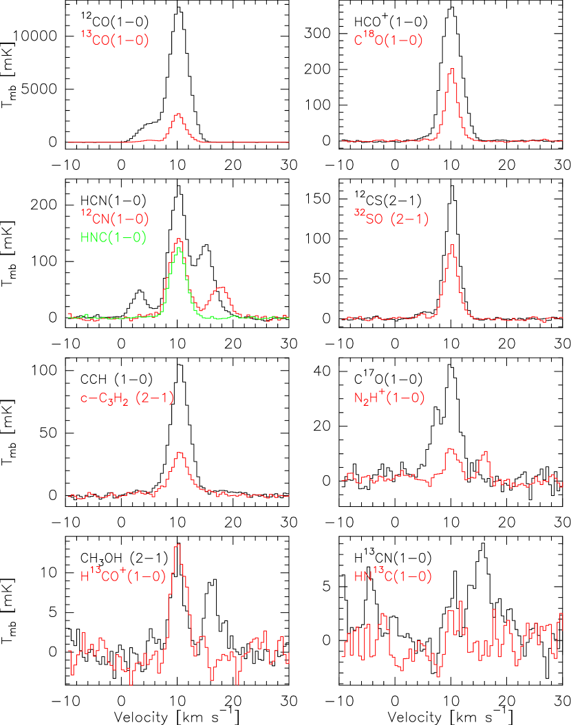
Figure 3: Spectra averaged over the mapped field of view.

Table 3: Line intensities and luminosities in the [-2,+18$\mathrm{\,km\,s^{-1}}$] velocity range and including all pixels.

Species	Simplifiedb	Completec	$A_{ij}$	$E_{\mathrm{u}}/k$	Intensity	Relative	Luminosity
	quantum numbers	quantum numbers	$\mathrm{\,s^{-1}}$	$\mathrm{\,K}$	$\mathrm{\,mK\,km\,s^{-1}}$	to $\mathrm{{}^{12}CO}$	$\mathrm{\,L_{\odot}}$
$\mathrm{{}^{12}CO}$	$1-0$	$J=1-0$	$7.2\times 10^{-8}$	5.5	60 430	100.00	1.0$\times 10^{-2}$
$\mathrm{{}^{13}CO}$	$1-0$	$J=1-0$	$3.2\times 10^{-8}$	5.3	9 198	15.22	1.4$\times 10^{-3}$
$\mathrm{HCO^{+}}$	$1-0$	$J=1-0$	$4.2\times 10^{-5}$	4.3	1 630	2.70	1.3$\times 10^{-4}$
$\mathrm{HCN}$	$1-0$	$J=1-0,F=2-1$	$2.4\times 10^{-5}$	4.3	1 540	2.55	1.2$\times 10^{-4}$
$\mathrm{CN}$	$1-0$	$N=1-0,J=3/2-1/2,F=5/2-3/2$	$1.2\times 10^{-5}$	5.4	776	1.28	1.3$\times 10^{-4}$
$\mathrm{C^{18}O}$	$1-0$	$J=1-0$	$6.3\times 10^{-8}$	5.3	556	0.92	8.0$\times 10^{-5}$
$\mathrm{{}^{12}CS}$	$2-1$	$J=2-1$	$1.7\times 10^{-5}$	7.0	513	0.85	5.3$\times 10^{-5}$
$\mathrm{C_{2}H}$	$1-0$	$N=1-0,J=3/2-1/2,F=2-1$	$1.5\times 10^{-6}$	4.2	457	0.76	3.2$\times 10^{-5}$
$\mathrm{HNC}$	$1-0$	$J=1-0,F=2-1$	$2.7\times 10^{-5}$	4.4	445	0.74	3.6$\times 10^{-5}$
$\mathrm{{}^{32}SO}$	$2-1$	$J=3-2,K=2-1$	$1.1\times 10^{-5}$	9.2	283	0.47	3.0$\times 10^{-5}$
$\mathrm{C^{17}O}$	$1-0$	$J=1-0,F=7/2-5/2$	$6.7\times 10^{-8}$	5.4	215	0.36	3.3$\times 10^{-5}$
$\mathrm{c-C_{3}H_{2}}$	$2-1$	$J=2-1,K_{+}=1-0,K_{-}=2-1$	$2.3\times 10^{-5}$	6.4	149	0.25	1.1$\times 10^{-5}$
$\mathrm{N_{2}H^{+}}$	$1-0$	$J=1-0,F1=2-1,F=3-2$	$3.6\times 10^{-5}$	4.5	67	0.11	6.0$\times 10^{-6}$
$\mathrm{CH_{3}OH}$	$2-1$	$J=2-1,K=0-0$	$3.4\times 10^{-6}$	7.0	65	0.11	6.4$\times 10^{-6}$
$\mathrm{H^{13}CN}$	$1-0$	$J=1-0,F=2-1$	$2.2\times 10^{-5}$	4.1	48	0.08	3.3$\times 10^{-6}$
$\mathrm{H^{13}CO^{+}}$	$1-0$	$J=1-0$	$3.9\times 10^{-5}$	4.2	25	0.04	1.8$\times 10^{-6}$
$\mathrm{HN^{13}C}$	$1-0$	$J=1-0,F=2-1$	$1.9\times 10^{-5}$	4.2	—	—	—
$\mathrm{SiO}$	$2-1$	$J=2-1$	$2.9\times 10^{-5}$	6.3	—	—	—

3.3 Mean line profiles over the observed field of view

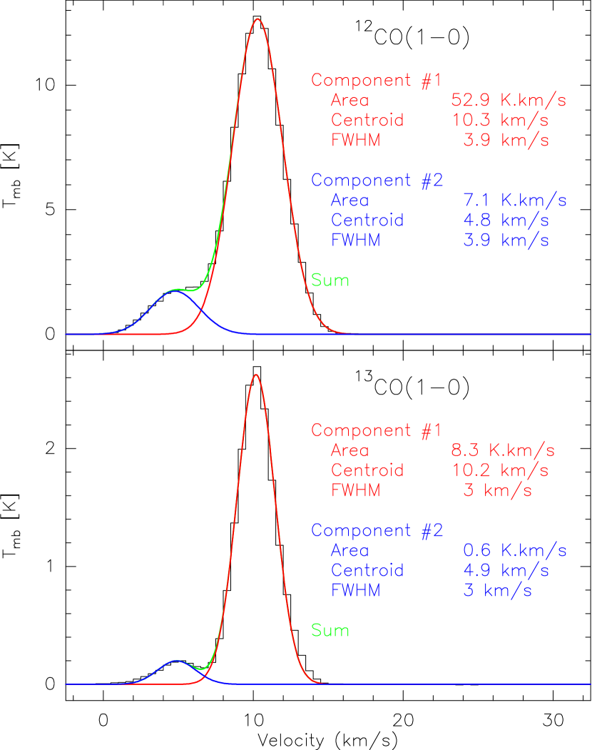
Figure 4: Gaussian fits of the two main velocity components that appears in the western edge of Orion B.

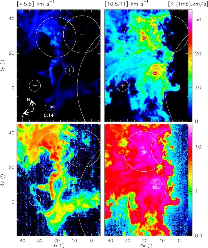
Figure 5: Spatial distribution of the $\mathrm{{}^{12}CO}$ $\mathrm{(1-0)}$ emission integrated over two different 0.5$\mathrm{\,km\,s^{-1}}$ velocity ranges in linear (top row) and logarithmic (bottom row) color scales.

Figure 3 shows the spectra of the main detected lines averaged over the mapped field of view. Several spectra show multiple components for different reasons. First, the multi-peak nature of the $\mathrm{CN}$, $\mathrm{HCN}$, $\mathrm{C^{17}O}$ and $\mathrm{N_{2}H^{+}}$ ground state lines is a consequence of the resolved hyperfine structure of these transitions. Second, the faintest spectra (e.g., $\mathrm{HN^{13}C}$) are detected at low signal-to-noise ratio, implying a noisy profile. Finally, the western side of the Orion B cloud displays two velocity components: The main one around 10.3$\mathrm{\,km\,s^{-1}}$ and a satellite one, ten times fainter, around 4.9$\mathrm{\,km\,s^{-1}}$. The two components have similar linewidth $(3-4\mathrm{\,km\,s^{-1}})$ and they overlap between 5 and 9.5$\mathrm{\,km\,s^{-1}}$. Figure 4 displays the fit for these two components on the $\mathrm{{}^{12}CO}$ and $\mathrm{{}^{13}CO}$ $\mathrm{(1-0)}$ spectra averaged over the field of view. The values of the $\mathrm{{}^{12}CO}$/$\mathrm{{}^{13}CO}$ integrated line intensity ratios are 6.4 and 11.8 for the main and the satellite components respectively. The difference in line ratios suggest that the satellite velocity component corresponds to lower column density material (see Section 6.1). The satellite component is barely detected in $\mathrm{C^{18}O}$, $\mathrm{HCO^{+}}$, and $\mathrm{{}^{12}CS}$, and it stays undetected for the other lines. Figure 5 shows the $\mathrm{{}^{12}CO}$ $\mathrm{(1-0)}$ emission in two channel maps belonging to the two velocity components, both in linear and logarithmic color scales. The use of a logarithmic transfer function shows that bright emission is surrounded by a halo of faint emission. This shows that the fainter velocity component still covers a large fraction of the observed surface.

We now argue that both velocity components along the line of sight are associated with the Orion B Giant Molecular Cloud. Figure 5 shows that the spatial distribution of both components overlap on most of the observed field, and that they are in close interaction with the massive stars of known distance, listed in Table 1. Furthermore, the 3-dimensional structure of interstellar extinction has been studied by Lallement et al. (2014) and Green et al. (2015) using differential reddening of stars at known distances. Towards Orion B, the reddening steeply increases between 300 and 500$\mathrm{\,pc}$, and most importantly, there is no significant reddening detected at closer or larger distances in this direction of the sky (Lallement, priv. comm.). These results are in excellent agreement with the distance determination of Orion through maser parallax (Menten et al., 2007). Overall the 3D structure of the Orion clouds is complex and could extend over several tens of parsec along the line of sight, a dimension comparable to the projected size on the plane of the sky.

Table 4 lists the integrated line intensities, $W^{\mathrm{}}$, and luminosities, $L$, computed as

$$\frac{L}{\mathrm{\,L_{\odot}}}=3.4\times 10^{-8}\left(\frac{3\mathrm{\,mm}}{\lambda}\right)^{3}\left(\frac{W^{\mathrm{}}}{1\mathrm{\,K\,km\,s^{-1}}}\right)\left(\frac{D}{400\mathrm{\,pc}}\right)\left(\frac{\Omega}{1^{\prime}\times 1^{\prime}}\right),$$

where $k_{\mathrm{bolt}}$ is Boltzmann constant, $\lambda$ the line rest wavelength, $D$ the source distance, and $\Omega$ the field-of-view angle. The dynamic range of reliable integrated intensity is about 2 400. Moreover, the typical intensity ratios of the $\mathrm{(1-0)}$ lines would be $\mathrm{{}^{12}CO}/\mathrm{{}^{13}CO}=6.7$, $\mathrm{{}^{13}CO}/\mathrm{C^{18}O}=16.7$, $\mathrm{C^{18}O}/\mathrm{{}^{12}CO}=0.9\%$, and $\mathrm{HCO^{+}}/\mathrm{{}^{12}CO}\sim\mathrm{HCN}/\mathrm{{}^{12}CO}\sim 3\%$. $\mathrm{{}^{12}CN}$, $\mathrm{C^{18}O}$, $\mathrm{{}^{12}CS}$, $\mathrm{C_{2}H}$, $\mathrm{HNC}$ emit about 1% of the $\mathrm{{}^{12}CO}$ intensity. The low-J lines of $\mathrm{{}^{32}SO}$, $\mathrm{C^{17}O}$, $\mathrm{c-C_{3}H_{2}}$, $\mathrm{N_{2}H^{+}}$, $\mathrm{H^{13}CN}$, $\mathrm{H^{13}CO^{+}}$ are up to 25 times fainter than the previous family, exemplified by $\mathrm{C^{18}O}$. The $\mathrm{HN^{13}C}$ and $\mathrm{SiO}$ integrated intensity can not be reliably measured.

3.4 CO-traced, dust-traced, and virial-traced mass and densities

In this section, we will compute the typical gas mass and densities using three common approaches: 1) the $\mathrm{{}^{12}CO}$ $\mathrm{(1-0)}$ luminosity, 2) the dust continuum luminosity, and 3) the virial theorem. Table 2 lists the found values.

The direct sum of the pixel intensity over the mapped field of view and between the $[-2,+18]\mathrm{\,km\,s^{-1}}$ velocity range indicates that the data cube contains a total CO luminosity of $\sim 2\,500\mathrm{\,K\,km\,s^{-1}\,pc^{2}}$. Using the standard CO-to-$\mathrm{H_{2}}$ conversion factor, $X_{\mathrm{CO}}=2.0\times 10^{20}\mathrm{\,cm^{-2}/(K\,km\,s^{-1})}$ or $4.35\mathrm{\,M_{\odot}}\mathrm{\,pc}^{-2}/(\mathrm{\,K\,km\,s^{-1}}{})$ (this includes the factor 1.36 to account for the presence of helium, Bolatto et al., 2013), this corresponds to a gas mass of $1.1\times 10^{4}\mathrm{\,M_{\odot}}$. The total surface covered was 0.86 square degree, i.e., $43\mathrm{\,pc}^{2}$. The mean intensity and mean surface density are $61\mathrm{\,K\,km\,s^{-1}}$ and $260\mathrm{\,M_{\odot}}\mathrm{\,pc}^{-2}$, respectively. The associated column density of gas is about $10^{22}\,\mathrm{H_{2}}\mathrm{\,cm^{-2}}$. This in turn gives a typical volume density of $40\mathrm{\,M_{\odot}}\mathrm{\,pc}^{-3}$ or 590 $\mathrm{H_{2}}$$\mathrm{\,cm^{-3}}$.

Using the Gould Belt Survey data and its SED fits, we can derive values for the same quantities from dust far infrared emission. To do this, we first used in section 2.4 a value different from the standard one for the conversion factor from $A_{\mathrm{K}}$ to $A_{\mathrm{V}}^{\mathrm{}}$ because 1) this is an observational quantity that can be measured relatively easily, and 2) we mainly deal with molecular gas, while the standard value is derived in diffuse gas. While this value depends on the optical properties (grain composition, grain shapes, and size distribution, which leads to the extinction curve) of the dust in Orion B, it is independent of any assumption about the gas properties. On the other hand, to derive the dust traced mass, we also need to use a value for the $N_{\mathrm{H}}$/$A_{\mathrm{V}}^{\mathrm{}}$ ratio. Assuming that the dependency of this ratio on the dust optical properties is only a second order effect, this ratio mainly depends on the gas-to-dust ratio, i.e., on how many grains there are per unit mass of gas. We thus use the standard value, $N_{\mathrm{H}}/A_{\mathrm{V}}^{\mathrm{}}=1.8\times 10^{21}\,\mathrm{H}\mathrm{\,cm^{-2}}\mathrm{\,mag}^{-1}$, for this ratio. This directly leads to a dust-traced mass of the mapped field of view of $\sim 3\,900\mathrm{\,M_{\odot}}$, a mean surface density of $92\mathrm{\,M_{\odot}}\mathrm{\,pc^{-2}}$ or $4\times 10^{21}\,\mathrm{H_{2}}\mathrm{\,cm^{-2}}$, and a mean volume density of $14\mathrm{\,M_{\odot}}\mathrm{\,pc^{-3}}$ or $210\,\mathrm{H_{2}}\mathrm{\,cm^{-3}}$.

The column density of neutral atomic hydrogen measured by integrating across profiles of the 21$\mathrm{\,cm}$ H i line taken by the LAB all-sky H i survey (Kalberla et al., 2005) is

$$N({H\textsc{i}})=1.823\times 10^{18}\mathrm{\,cm^{-2}}\int T_{B}dv\approx(1.8\pm 0.2)\times 10^{21}\mathrm{\,cm^{-2}}$$

in the optically thin limit. This corresponds to approximately $1.0\mathrm{\,mag}$ of visual extinction using the usual conversion $N_{\mathrm{H}}/E_{\mathrm{B-V}}=5.8\times 10^{21}\mathrm{\,cm^{-2}}\,\mathrm{\,mag}^{-1}$ derived by Bohlin et al. (1978) and $R_{\mathrm{V}}^{\mathrm{}}=E_{\mathrm{B-V}}/A_{\mathrm{V}}^{\mathrm{}}=3.1$. The total expected foreground gas contribution for a source at a distance of 400$\mathrm{\,pc}$ is $N_{\mathrm{H}}=1.2\times 10^{21}\mathrm{\,cm^{-2}}$ for a local mean gas density $\langle n(\mathrm{H})\rangle=1.15\mathrm{\,cm^{-3}}$ (Spitzer, 1978) corresponding to $A_{\mathrm{V}}^{\mathrm{}}=0.75\mathrm{\,mag}$ using the same conversion from column density to extinction. The minimum value of the visual extinction across the observed field of view, (i.e., 0.7) is therefore in good agreement with the expected contribution of diffuse material along the line of sight. As the mean visual extinction is 4.7$\mathrm{\,mag}$, correcting for this diffuse component would result in decreasing the molecular part of the dust-traced mass and densities by less than 20%. We choose to consider this difference negligible, i.e., to consider that all the dust-traced mass refers to gas where hydrogen is molecular.

Following Solomon et al. (1987) and Bolatto et al. (2013), we can also compute a mass assuming that turbulent pressure and gravity are in virial equilibrium. Bolatto et al. (2013) indicate that the virial mass, $M_{\mathrm{vir}}^{\mathrm{}}$, is given by

$$M_{\mathrm{vir}}^{\mathrm{}}=f\,R\,\sigma^{2},$$ (5)

where $R$ is the projected radius of the measured field of view, $\sigma$ is the 1D velocity dispersion (full width at half maximum of a Gaussian divided by 2.35), and $f$ a factor that takes into account projection effects. This factor depends on the assumed density profile of the GMC. For a spherical volume density distribution with a power-law index $k$, i.e.,

$$\rho(r)\propto r^{-k},$$ (6)

$f$ is 1 160, 1 040, and $700\mathrm{\,\mathrm{\,M_{\odot}}\mathrm{\,pc}^{-1}(\mathrm{\,km\,s^{-1}})^{-2}}$, for $k=0$, 1, and 2, respectively. In our case, $R\simeq 0.5\,\sqrt{5.6\times 7.5}=3.3$, and $\sigma\simeq 3.9/2.35=1.7\mathrm{\,km\,s^{-1}},$ when we only take into account the Gaussian fit of the main velocity component around 10.5$\mathrm{\,km\,s^{-1}}$. We thus obtain a virial mass between 6 200 and 9 500$\mathrm{\,M_{\odot}}$.

We find that, contrary to expectations, the CO-traced mass is typically 3 times the dust-traced mass, and that the virial mass is lower than the CO-traced mass but it is much higher than the dust-traced mass. Throughout the paper, we will propose that this discrepancy is related to the strong far UV illumination of the mapped field of view (see Section 3.1). In the meantime, we will take an average between the CO-traced and dust-traced mass and densities when we will need an order of magnitude estimate for these quantities.

4 Fraction of line fluxes from different gas regimes

Table 4: Properties of the $A_{\mathrm{V}}^{\mathrm{}}$ masks sorted by increasing range of visual extinction.

Parameter	Unit	$1\leq A_{\mathrm{V}}^{\mathrm{}}<2$	$2\leq A_{\mathrm{V}}^{\mathrm{}}<6$	$6\leq A_{\mathrm{V}}^{\mathrm{}}<15$	$15\leq A_{\mathrm{V}}^{\mathrm{}}<222$
$W^{\mathrm{min}}_{\mathrm{CO}}-W^{\mathrm{mean}}_{\mathrm{CO}}-W^{\mathrm{max}}_{\mathrm{CO}}$	$\mathrm{\,K\,km\,s^{-1}}$	$0-6.8-46.9$	$1.3-62.6-211$	$24.8-122-261$	$41.5-137-288$
$A_{\mathrm{V}}^{\mathrm{min}}-A_{\mathrm{V}}^{\mathrm{mean}}-A_{\mathrm{V}}^{\mathrm{max}}$	$\mathrm{\,mag}$	$1-1.4-2$	$2-3.6-6$	$6-8.5-15$	$15-28.9-222$
$T_{\mathrm{d}}^{\mathrm{min}}-T_{\mathrm{d}}^{\mathrm{mean}}-T_{\mathrm{d}}^{\mathrm{max}}$	$\mathrm{\,K}$	$19-24-45$	$19-26-67$	$18-29-99$	$16-26-95$
$G_{0}^{\mathrm{min}}-G_{0}^{\mathrm{mean}}-G_{0}^{\mathrm{max}}$	ISRF (Habing, 1968)	$8.9-30-680$	$8.4-46-5100$	$6-72-36000$	$4-47-28000$
CO-traced mass	$\mathrm{\,M_{\odot}}$	$320$ $(3\%)$	$5600$ $(51\%)$	$4400$ $(40\%)$	$830$ $(8\%)$
Dust-traced mass	$\mathrm{\,M_{\odot}}$	$300$ $(8\%)$	$1500$ $(38\%)$	$1400$ $(36\%)$	$790$ $(20\%)$
Emitting surface	$\mathrm{\,pc}^{2}$	$11$ $(25\%)$	$21$ $(48\%)$	$8.4$ $(20\%)$	$1.4$ $(3.3\%)$
Typical volume	$\mathrm{\,pc}^{3}$	$36$ $(13\%)$	$93$ $(33\%)$	$24$ $(8.6\%)$	$1.7$ $(0.6\%)$
CO-traced mean column density	$\mathrm{\,M_{\odot}}\mathrm{\,pc}^{-2}|10^{21}\mathrm{H_{2}}{}\mathrm{\,cm^{-2}}$	$30$ — $1.4$	$270$ — $12$	$530$ — $24$	$590$ — $27$
Dust-traced mean column density	$\mathrm{\,M_{\odot}}\mathrm{\,pc}^{-2}|10^{21}\mathrm{H_{2}}{}\mathrm{\,cm^{-2}}$	$28$ — $1.3$	$71$ — $3.3$	$160$ — $7.6$	$560$ — $26$
CO-traced mean volume density	$\mathrm{\,M_{\odot}}\mathrm{\,pc}^{-3}|\mathrm{H_{2}}{}\mathrm{\,cm^{-3}}$	$8.9$ — $130$	$60$ — $890$	$180$ — $2700$	$500$ — $7500$
Dust-traced mean volume density	$\mathrm{\,M_{\odot}}\mathrm{\,pc}^{-3}|\mathrm{H_{2}}{}\mathrm{\,cm^{-3}}$	$8.4$ — $130$	$16$ — $230$	$57$ — $850$	$470$ — $7100$

Table 5: Percentage of the total line fluxes inside the four $A_{\mathrm{V}}^{\mathrm{}}$ mask regions, integrated over $[9,12\mathrm{\,km\,s^{-1}}]$.

Species	Transition	$0\leq A_{\mathrm{V}}^{\mathrm{}}<222$	$1\leq A_{\mathrm{V}}^{\mathrm{}}<2$	$2\leq A_{\mathrm{V}}^{\mathrm{}}<6$	$6\leq A_{\mathrm{V}}^{\mathrm{}}<15$	$15\leq A_{\mathrm{V}}^{\mathrm{}}<222$
$\mathrm{{}^{12}CO}$	$1-0$	$100\%$	$2.5\%$	$52\%$	$38\%$	$7.6\%$
$\mathrm{C_{2}H}$	$1-0$	$100\%$	$4.4\%$	$41\%$	$37\%$	$17\%$
$\mathrm{c-C_{3}H_{2}}$	$2-1$	$100\%$	$4.5\%$	$40\%$	$38\%$	$17\%$
$\mathrm{HCO^{+}}$	$1-0$	$100\%$	$2.8\%$	$41\%$	$40\%$	$16\%$
$\mathrm{{}^{13}CO}$	$1-0$	$100\%$	$1.4\%$	$38\%$	$45\%$	$15\%$
$\mathrm{HCN}$	$1-0$	$100\%$	$1.7\%$	$36\%$	$44\%$	$18\%$
$\mathrm{{}^{12}CN}$	$1-0$	$100\%$	$2.6\%$	$33\%$	$45\%$	$19\%$
$\mathrm{HNC}$	$1-0$	$100\%$	$2.1\%$	$29\%$	$41\%$	$27\%$
$\mathrm{C^{17}O}$	$1-0$	$100\%$	$5.6\%$	$25\%$	$43\%$	$26\%$
$\mathrm{{}^{12}CS}$	$2-1$	$100\%$	$0.68\%$	$25\%$	$42\%$	$32\%$
$\mathrm{{}^{32}SO}$	$2-1$	$100\%$	$0.86\%$	$24\%$	$44\%$	$31\%$
$\mathrm{C^{18}O}$	$1-0$	$100\%$	$0.49\%$	$23\%$	$48\%$	$29\%$
$\mathrm{CH_{3}OH}$	$2-1$	$99\%$	$4.4\%$	$5.8\%$	$41\%$	$48\%$
$\mathrm{H^{13}CO^{+}}$	$1-0$	$98\%$	$0.67\%$	$7.1\%$	$34\%$	$56\%$
$\mathrm{N_{2}H^{+}}$	$1-0$	$100\%$	$-11\%$	$8.2\%$	$17\%$	$88\%$

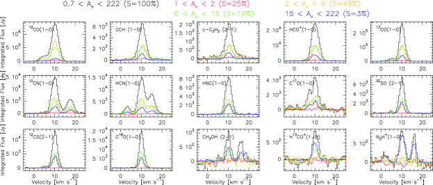
Figure 6: Left: Spatial distribution of the four following masks: $1\leq A_{\mathrm{V}}^{\mathrm{}}<2$ in red, $2\leq A_{\mathrm{V}}^{\mathrm{}}<6$ in orange, $6\leq A_{\mathrm{V}}^{\mathrm{}}<15$ in green, and $15\leq A_{\mathrm{V}}^{\mathrm{}}<222$ in blue. The percentages in the legend list the fraction of the surface contained in the different masks. Right: Flux integrated over the masks as a function of velocity. The spectra of different color show the evolution of the flux in each line as a function of the mask used: All pixels observed in black, all pixels with $1\leq A_{\mathrm{V}}^{\mathrm{}}<2$ in red, $2\leq A_{\mathrm{V}}^{\mathrm{}}<6$ in orange, all pixels with $6\leq A_{\mathrm{V}}^{\mathrm{}}<15$ in green, and all pixels with $15\leq A_{\mathrm{V}}^{\mathrm{}}<222$ in blue.

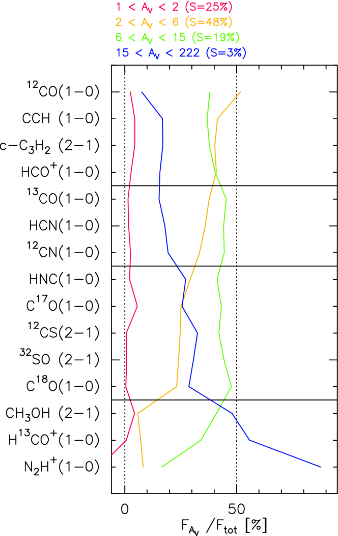
Figure 7: For each line, flux integrated over each of the four $A_{\mathrm{V}}^{\mathrm{}}$ mask divided by the flux computed over the observed field of view. All fluxes are computed between 9 and 12$\mathrm{\,km\,s^{-1}}$. The black horizontal lines define the groups of lines described in Section 4.1.

In this section, we will explore which fraction of the line fluxes comes from more or less dense gas, and from more or less far UV illuminated gas.

4.1 Flux profiles over different $A_{\mathrm{V}}^{\mathrm{}}$ ranges

We chose 4 ranges of $A_{\mathrm{V}}^{\mathrm{}}$, representing diffuse $(1\leq A_{\mathrm{V}}^{\mathrm{}}<2)$, and translucent $(2\leq A_{\mathrm{V}}^{\mathrm{}}<6)$ gas, the environment of filaments ($6\leq A_{\mathrm{V}}^{\mathrm{}}<15$), and dense gas ($15\leq A_{\mathrm{V}}^{\mathrm{}}$). Table 4 lists the physical properties of the different regions based on their $\mathrm{{}^{12}CO}$ $\mathrm{(1-0)}$ and far infrared emission. While the different regions have by construction increasing values of their mean visual extinction (1.4, 4, 9, and 29, respectively), they present similar mean dust temperature and far UV illumination. As expected the minimum dust temperature decreases when the range of visual extinction increases. In contrast, the maximum dust temperatures, and thus far UV illuminations, are also found in the masks of highest visual extinctions. This is related to the presence of very dense (probably cold) molecular gas in front of young massive stars that excite H ii regions (see, e.g., the dark filament in front of IRS2 that excites the NGC 2024 nebula). This could also be due to the presence of embedded heating sources.

Contrary to standard expectations, the dust and CO-traced mass are similar for diffuse and dense regions, while they differ by a factor 3 mostly in the translucent gas and filament environment. Moreover, both the dust and CO-traced matter indicate that about 50% of the gas lies in diffuse and translucent gas. Dense cores $(15\leq A_{\mathrm{V}}^{\mathrm{}})$ represent between 10 and 20% of the mass but only 3% of the surface and 0.6% of the volume. The sum of the volume fractions of the 4 regions only amounts to 55% because of the simplified way the volumes are computed $(V=S^{3/2})$. This implies that volume densities can only be interpreted as typical values. Finally, the volume densities increase from $\sim 100$ to $7\,300\,\mathrm{H_{2}}\mathrm{\,cm^{-3}}$ for diffuse and dense gas, respectively. Translucent gas and the environment of filaments have typical density values of $\sim 500$ and $1\,500\,\mathrm{H_{2}}\mathrm{\,cm^{-3}}$, respectively. The volume density increases by a factor $3-5$ from each gas regime to the next. We will use this fact to statistically identify high/low $A_{\mathrm{V}}^{\mathrm{}}$ lines of sight with high/low density gas, respectively.

Figure 6 presents the $A_{\mathrm{V}}^{\mathrm{}}$ masks and it displays the flux profiles integrated over regions of different extinction ranges. To better quantify the different behavior of the fluxes integrated over these different regions, Table 5 and Fig. 7 present, for each line, the percentage of the total line flux that comes from the different $A_{\mathrm{V}}^{\mathrm{}}$ masked regions $(F_{A_{\mathrm{V}}^{\mathrm{}}}/F_{\mathrm{tot}})$. In all cases, the fluxes are integrated in the $[9,12\mathrm{\,km\,s^{-1}}]$ velocity range. The lines were sorted by increasing value of the $F(1\leq A_{\mathrm{V}}^{\mathrm{}}<2)+F(2\leq A_{\mathrm{V}}^{\mathrm{}}<6)$ ratio. This value represents for each line the flux coming from both diffuse and translucent gas. The layout of the panels in Fig. 6 also follows this order. We can group the lines in 4 categories depending on how the line flux is divided between regions of very low ($1\leq A_{\mathrm{V}}^{\mathrm{}}<2$), low ($2\leq A_{\mathrm{V}}^{\mathrm{}}<6$), intermediate ($6\leq A_{\mathrm{V}}^{\mathrm{}}<15$), or high $(15\leq A_{\mathrm{V}}^{\mathrm{}})$ visual extinction.

In the first category of lines, the regions of low and intermediate visual extinctions contribute more than $\sim 45\%$ of the total flux, and regions of high visual extinction contributes less than $\sim 20\%$ of the flux. In this category, the total flux is predominantly coming from translucent lines of sight $(2\leq A_{\mathrm{V}}^{\mathrm{}}<6)$. This is the case of the $\mathrm{(1-0)}$ lines of $\mathrm{{}^{12}CO}$, $\mathrm{HCO^{+}}$, $\mathrm{C_{2}H}$, and the $\mathrm{c-C_{3}H_{2}}$ ($2-1$) line. From these species, $\mathrm{{}^{12}CO}$ is the one with the largest contribution (55%) from diffuse and translucent gas ($A_{\mathrm{V}}^{\mathrm{}}\leq 6$).

In the 2nd category, the total flux is now predominantly coming from regions of intermediate visual extinction $(45\%$ coming from $6\leq A_{\mathrm{V}}^{\mathrm{}}<15)$. But the diffuse and translucent gas still contributes for a similar fraction $(35-40\%)$ of the total flux, and dense gas do not contribute more than 20% of the total flux. This is the case of the $\mathrm{(1-0)}$ lines of $\mathrm{{}^{13}CO}$, HCN, and CN.

In the third category, the flux comes predominantly from regions of intermediate visual extinction as in the 2nd category. But the regions of low and high visual extinctions both contribute for similar fractions of the total flux (around 30%). The $\mathrm{(1-0)}$ lines of HNC, $\mathrm{C^{18}O}$, $\mathrm{C^{17}O}$, and the lines of the sulfur species, namely the $\mathrm{(2-1)}$ line of $\mathrm{{}^{12}CS}$, and $\mathrm{{}^{32}SO}$, belong to this category.

The $\mathrm{(1-0)}$ lines of $\mathrm{N_{2}H^{+}}$ and $\mathrm{H^{13}CO^{+}}$, as well as the $\mathrm{(2-1)}$ lines of $\mathrm{CH_{3}OH}$ form the last category. In this one, the flux is predominantly coming from the regions of high visual extinctions $(15\leq A_{\mathrm{V}}^{\mathrm{}})$. These lines all present a small surface filling factor $(\la 5\%)$ and negligible contribution from the translucent and diffuse gas. In this category, $\mathrm{N_{2}H^{+}}$ plays a special role. This is the only easily mapped line, where the flux is completely dominated (at 88%) by regions of high visual extinctions, probably dense cores.

4.2 Flux profiles over different $T_{\mathrm{d}}^{\mathrm{}}$ ranges

Table 6: Properties of the $T_{\mathrm{d}}^{\mathrm{}}$ masks sorted by increasing range of dust temperature.

Parameter	Unit	$16\leq T_{\mathrm{d}}^{\mathrm{}}<19.5$	$19.5\leq T_{\mathrm{d}}^{\mathrm{}}<23.5$	$23.5\leq T_{\mathrm{d}}^{\mathrm{}}<32$	$32\leq T_{\mathrm{d}}^{\mathrm{}}<100$
$W^{\mathrm{min}}_{\mathrm{CO}}-W^{\mathrm{mean}}_{\mathrm{CO}}-W^{\mathrm{max}}_{\mathrm{CO}}$	$\mathrm{\,K\,km\,s^{-1}}$	$0.2-63.8-149$	$0-46.5-197$	$0-57.4-273$	$0.2-114-288$
$A_{\mathrm{V}}^{\mathrm{min}}-A_{\mathrm{V}}^{\mathrm{mean}}-A_{\mathrm{V}}^{\mathrm{max}}$	$\mathrm{\,mag}$	$1.1-17.2-127$	$0.7-4-69$	$0.8-4.1-222$	$0.8-7.2-186$
$T_{\mathrm{d}}^{\mathrm{min}}-T_{\mathrm{d}}^{\mathrm{mean}}-T_{\mathrm{d}}^{\mathrm{max}}$	$\mathrm{\,K}$	$16-19-20$	$20-22-24$	$24-27-32$	$32-40-99$
$G_{0}^{\mathrm{min}}-G_{0}^{\mathrm{mean}}-G_{0}^{\mathrm{max}}$	ISRF (Habing, 1968)	$4-8.6-10$	$10-18-26$	$26-50-120$	$120-400-36000$
CO-traced mass	$\mathrm{\,M_{\odot}}$	$220$ $(2\%)$	$3900$ $(35\%)$	$4300$ $(39\%)$	$2700$ $(25\%)$
Dust-traced mass	$\mathrm{\,M_{\odot}}$	$260$ $(7\%)$	$1500$ $(38\%)$	$1400$ $(36\%)$	$770$ $(20\%)$
Emitting surface	$\mathrm{\,pc}^{2}$	$0.8$ $(1.8\%)$	$19$ $(45\%)$	$18$ $(41\%)$	$5.5$ $(13\%)$
Typical volume	$\mathrm{\,pc}^{3}$	$0.7$ $(0.3\%)$	$84$ $(30\%)$	$73$ $(26\%)$	$13$ $(4.6\%)$
CO-traced mean column density	$\mathrm{\,M_{\odot}}\mathrm{\,pc}^{-2}|10^{21}\mathrm{H_{2}}{}\mathrm{\,cm^{-2}}$	$280$ — $13$	$200$ — $9.3$	$250$ — $12$	$490$ — $23$
Dust-traced mean column density	$\mathrm{\,M_{\odot}}\mathrm{\,pc}^{-2}|10^{21}\mathrm{H_{2}}{}\mathrm{\,cm^{-2}}$	$330$ — $16$	$78$ — $3.6$	$81$ — $3.7$	$140$ — $6.4$
CO-traced mean volume density	$\mathrm{\,M_{\odot}}\mathrm{\,pc}^{-3}|\mathrm{H_{2}}{}\mathrm{\,cm^{-3}}$	$310$ — $4600$	$46$ — $690$	$59$ — $890$	$210$ — $3100$
Dust-traced mean volume density	$\mathrm{\,M_{\odot}}\mathrm{\,pc}^{-3}|\mathrm{H_{2}}{}\mathrm{\,cm^{-3}}$	$380$ — $5600$	$18$ — $270$	$19$ — $290$	$59$ — $890$

Table 7: Percentage of the total line fluxes inside the four $T_{\mathrm{d}}^{\mathrm{}}$ mask regions, integrated over $[9,12\mathrm{\,km\,s^{-1}}]$.

Species	Transition	$16\leq T_{\mathrm{d}}^{\mathrm{}}<100$	$16\leq T_{\mathrm{d}}^{\mathrm{}}<19.5$	$19.5\leq T_{\mathrm{d}}^{\mathrm{}}<23.5$	$23.5\leq T_{\mathrm{d}}^{\mathrm{}}<32$	$32\leq T_{\mathrm{d}}^{\mathrm{}}<100$
$\mathrm{C_{2}H}$	$1-0$	$100\%$	$3.2\%$	$25\%$	$39\%$	$32\%$
$\mathrm{c-C_{3}H_{2}}$	$2-1$	$100\%$	$4.2\%$	$25\%$	$39\%$	$31\%$
$\mathrm{{}^{12}CN}$	$1-0$	$100\%$	$4\%$	$27\%$	$33\%$	$36\%$
$\mathrm{HCN}$	$1-0$	$100\%$	$4.2\%$	$29\%$	$34\%$	$32\%$
$\mathrm{HCO^{+}}$	$1-0$	$100\%$	$4.6\%$	$30\%$	$36\%$	$29\%$
$\mathrm{HNC}$	$1-0$	$100\%$	$7.9\%$	$31\%$	$32\%$	$29\%$
$\mathrm{{}^{12}CO}$	$1-0$	$100\%$	$2.4\%$	$38\%$	$38\%$	$22\%$
$\mathrm{{}^{12}CS}$	$2-1$	$100\%$	$8.4\%$	$35\%$	$28\%$	$29\%$
$\mathrm{{}^{13}CO}$	$1-0$	$100\%$	$4.6\%$	$41\%$	$33\%$	$21\%$
$\mathrm{{}^{32}SO}$	$2-1$	$100\%$	$11\%$	$38\%$	$28\%$	$23\%$
$\mathrm{H^{13}CO^{+}}$	$1-0$	$100\%$	$16\%$	$33\%$	$24\%$	$26\%$
$\mathrm{C^{17}O}$	$1-0$	$100\%$	$7.9\%$	$44\%$	$29\%$	$19\%$
$\mathrm{CH_{3}OH}$	$2-1$	$100\%$	$18\%$	$35\%$	$29\%$	$18\%$
$\mathrm{C^{18}O}$	$1-0$	$100\%$	$9.1\%$	$44\%$	$27\%$	$20\%$
$\mathrm{N_{2}H^{+}}$	$1-0$	$100\%$	$27\%$	$39\%$	$15\%$	$20\%$

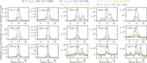
Figure 8: Left: Spatial distribution of the four following masks: $16\leq T_{\mathrm{d}}^{\mathrm{}}<19.5\mathrm{\,K}$ in blue, $19.5\leq T_{\mathrm{d}}^{\mathrm{}}<23.5\mathrm{\,K}$ in green, $23.5\leq T_{\mathrm{d}}^{\mathrm{}}<32\mathrm{\,K}$ in orange, and $32\leq T_{\mathrm{d}}^{\mathrm{}}<100\mathrm{\,K}$ in red. The percentages in the legend list the fraction of the surface contained in the different masks. Right: Flux integrated over the masks as a function of velocity. The spectrum of different colors the evolution of the flux for the same line as a function of the used mask: All pixels observed in black, all pixels with $16\leq T_{\mathrm{d}}^{\mathrm{}}<19.5\mathrm{\,K}$ in blue, all pixels with $19.5\leq T_{\mathrm{d}}^{\mathrm{}}<23.5\mathrm{\,K}$ in green, all pixels with $23.5\leq T_{\mathrm{d}}^{\mathrm{}}<32\mathrm{\,K}$ in orange, and all pixels with $32\leq T_{\mathrm{d}}^{\mathrm{}}<100\mathrm{\,K}$ in red.

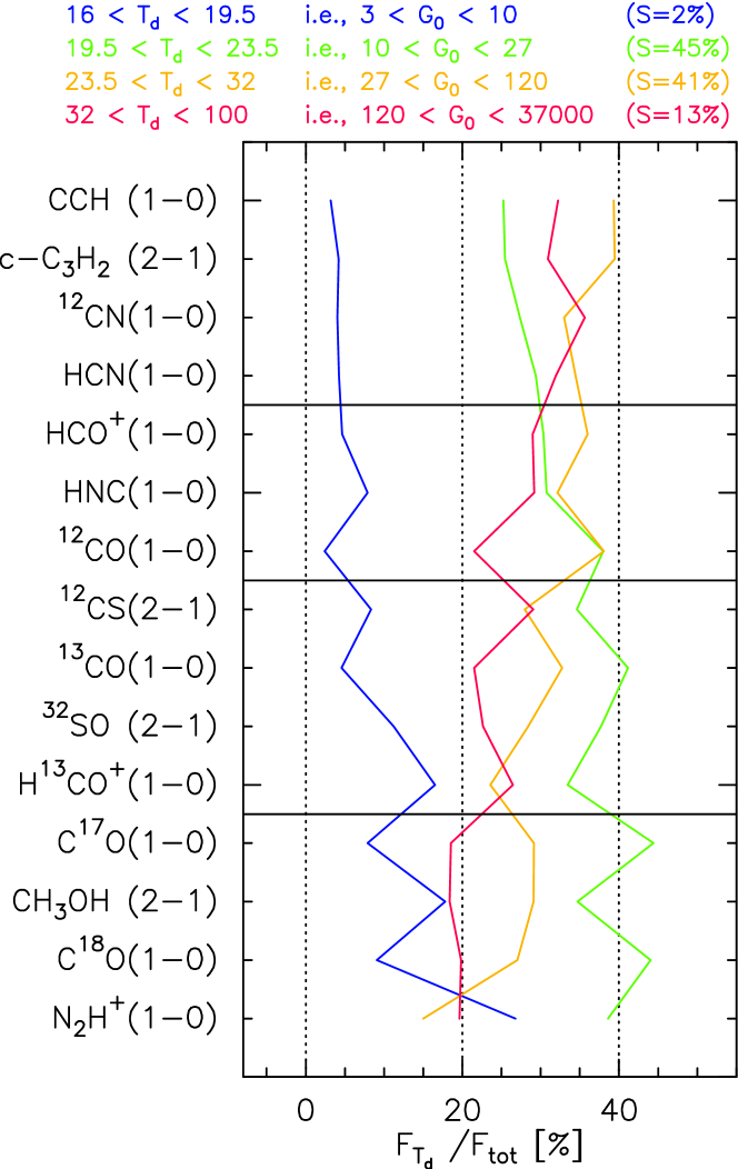
Figure 9: For each line, flux integrated over each of the four $T_{\mathrm{d}}^{\mathrm{}}$ masks divided by the flux integrated over the observed field of view. All fluxes are computed between 9 and 12$\mathrm{\,km\,s^{-1}}$. The black horizontal lines define the groups of lines described in Section 4.2.

We chose 4 ranges of $T_{\mathrm{d}}^{\mathrm{}}$, representing cold dust $(16\leq T_{\mathrm{d}}^{\mathrm{}}<19.5\mathrm{\,K})$ that corresponds to gas that is shielded from the UV field (e.g., the dense cores), lukewarm dust $(19.5\leq T_{\mathrm{d}}^{\mathrm{}}<23.5\mathrm{\,K})$, warm dust $(23.5\leq T_{\mathrm{d}}^{\mathrm{}}<32\mathrm{\,K})$, and hot dust $(32\leq T_{\mathrm{d}}^{\mathrm{}}<100\mathrm{\,K})$. It is clear that this fitted dust temperature is biased toward the presence of warm dust because the dust emissivity increases rapidly with the temperature in the far infrared. Hence, cool dense gas is probably present along the line of sight of highest extinction, even though the fitted dust temperature is relatively high.

We here use the dust temperature as a proxy for the typical far UV illumination along the line of sight (see Section 2.4). In fact, using Eq. 3, we obtain that the mean far UV illumination is 9, 18, 50, and 400 for the cold, lukewarm, warm, and hot dust masks, respectively. This implies very different kinds of PDRs present along the line of sight. Moreover, the 4 masks of dust temperature display a morphology very different from that of the masks of visual extinction. Only the dense cores in Horsehead and near NGC 2023 are clearly delineated in both families of masks, while the intermediate density filamentary structure and diffuse/translucent gas are present in all 4 masks of dust temperature. Instead, the morphology of these temperature masks coincides well with the boundaries of the different H ii regions. We thus interpret the cold, lukewarm, warm, and hot dust masks as very low, low, medium, and high far UV illumination masks.

The field of view is dominated by intermediate far UV illumination PDRs (83% of the surface have a $G_{0}^{\mathrm{}}$ between 10 and 120). Less than 2% of the lines of sight have $G_{0}^{\mathrm{}}\leq 10$ and about 15% have $G_{0}^{\mathrm{}}>120$. Moreover, the CO-traced mass is 0.86, 2.6, 3.1, and 3.5 times the dust-traced mass in the cold, lukewarm, warm, and hot dust regions. Similar ratios are found for the volume densities. This confirms that the discrepancy between CO and dust traced mass is linked to the enhanced far UV illumination of the South-Western edge of Orion B.

Figure 8 presents the $T_{\mathrm{d}}^{\mathrm{}}$ masks and it displays the flux profiles integrated over regions of different far UV illumination. To better quantify the different behavior of the fluxes integrated over these different regions, Table 6 and Fig. 9 presents, for each line, the percentage of the total line flux that comes from the different $T_{\mathrm{d}}^{\mathrm{}}$ masked regions $100\,(F_{T_{\mathrm{d}}^{\mathrm{}}}/F_{\mathrm{tot}})$. In all cases, the fluxes are integrated in the $[9,12\mathrm{\,km\,s^{-1}}]$ velocity range. The lines were sorted by decreasing distance between the sum of the flux coming from the highest far UV illumination regions (red and orange masks) and the sum of the flux coming from the lowest far UV illumination regions (green and blue masks). The layout of the panels in Fig. 8 also follows this order. While oscillations on the 4 individual curves of Fig. 9 are present, the general tendency is that the percent of flux coming from the highest far UV illuminated regions decreases from top to bottom. We can thus group the lines in 4 categories depending on whether the line flux comes predominantly from the very low, low, medium, or high far UV illumination regions.

In the first category, the regions of high far UV illumination $(G_{0}^{\mathrm{}}>27)$ contribute about 70% of the total line flux and the region of very low illumination $(G_{0}^{\mathrm{}}<10)$ contributes less than 5%. High $(G_{0}^{\mathrm{}}>120)$ and medium $(27<G_{0}^{\mathrm{}}<120)$ illumination regions contribute about equally to the total flux. The fundamental lines of the $\mathrm{C_{2}H}$, $\mathrm{c-C_{3}H_{2}}$, $\mathrm{{}^{12}CN}$, and $\mathrm{HCN}$ belong to this category.

In the second category, containing the $\mathrm{HCO^{+}}$, $\mathrm{HCN}$ and $\mathrm{{}^{12}CO}$ $\mathrm{(1-0)}$ lines, the line flux comes predominantly $(65-75\%)$ comes from intermediate far UV illumination regions $(10<G_{0}^{\mathrm{}}<120)$. The highest illumination region still contributes for $20-30\%$ of the total flux, while lowest illumination region contributes for less than 10%.

In the third category, the flux comes first from the region where $10<G_{0}^{\mathrm{}}<27$. Quantitatively, this is the category where the flux coming from $G_{0}^{\mathrm{}}<27$ starts to dominates compared to medium and intermediate illumination regions. The $\mathrm{(1-0)}$ line of $\mathrm{{}^{13}CO}$ and $\mathrm{H^{13}CO^{+}}$, as well as the $\mathrm{(2-1)}$ line of $\mathrm{{}^{12}CS}$, and $\mathrm{{}^{32}SO}$ belong to this category.

In the last category, the flux coming from regions where $G_{0}^{\mathrm{}}<27$ contributes between 52 and 66% of the total flux. This contains the $\mathrm{CH_{3}OH}$ $\mathrm{(2-1)}$, and the $\mathrm{(1-0)}$ line of the rarest CO isotopologues and $\mathrm{N_{2}H^{+}}$.

5 Molecular low-J lines as a probe of the column density

5.1 Visual extinction vs. line integrated intensities

Figure 10: Joint distributions of the visual extinction as a function of the line integrated intensity for a selection of the detected lines. The percentage in the top left corner indicates the surface over which the joint distributions can be reliably computed. These distributions contains both the global trend for the bulk of the gas and extreme behavior at low and high visual extinctions. The number of sightlines falling in a given 2D bin of the distribution is color-coded using a logarithmic scale to emphasize the extreme behavior (in particular the dense cores) that occupy a small fraction of the observed field of view. In contrast, the white rectangle displays the region of the distribution where 90% of the points are located: 2.5% of the points are outside this rectangle on each side. This allows us to define more robust global trends for the bulk of the gas. The white point shows the median of the two marginalized distributions. A line of unit slope, i.e., a linear relationship between visual extinction and the line integrated intensities, is overlaid as the white plain line going through the white cross. The black points show the median values of all data points falling in an interval regularly sampled of the logarithm of the line integrated intensity. The black error bars show the range of values where 50% of the points in the current bin are located. This allows us to ask whether molecular lines are a good tracers of the visual extinction. All these parameters are listed in Table 7. The red, orange, green, and blue horizontal dashed lines show the visual extinction limits (1, 2, 6, and 15 magnitudes, respectively) used in the masks of Fig. 6. This enables us to visualize the amount of well detected pixels that falls in each of the masks for each line.

Figure 10 presents the joint distributions of the visual extinction and line integrated intensities for the studied molecular tracers. As the visual extinction is proportional to the amount of matter along the line of sight, it is desirable to make a comparison of all the matter traced by the molecules along this line of sight. Hence, the line profiles are integrated over the full velocity range where the line is measured, i.e., not just integrated anymore on the [9,12$\mathrm{\,km\,s^{-1}}$] velocity range. The visual extinctions are defined over the full field of view. In contrast, the line integrated intensities are well defined for only a fraction of the field of view. The joint distributions were thus only computed where the line integrated intensities are well defined (the criteria can be found in Section 2.5). For each distribution, the additional statistics (in particular for the visual extinction) are computed on this fraction of points. Table 7 lists these statistics.

The first obvious trend in Fig. 10 is the global correlation between the visual extinction, $A_{\mathrm{V}}^{\mathrm{}}$, and the line integrated intensities, $W^{\mathrm{}}$. This correlation is clearly visualized through the comparison of the black curves, which show the typical behavior of the variations of $A_{\mathrm{V}}^{\mathrm{}}$ as a function of $W^{\mathrm{}}$, with the white lines that represent a linear relation between these two quantities. While the lines are often overly bright with respect to the white line at low extinction, and their integrated intensity sometimes saturate at high visual extinction, a correlation is clearly present for a large fraction of the measured lines of sight between these two regimes. More precisely, the $\mathrm{C^{18}O}$, and $\mathrm{HNC}$ $\mathrm{(1-0)}$ lines are the best tracers of the visual extinctions when the integrated line intensity is above 1$\mathrm{\,K\,km\,s^{-1}}$. Indeed, there is an excellent agreement between the black line and the white line when $W^{\mathrm{}}$ is above the intensity median value, and the scatter is low around these curves for both transitions. The $\mathrm{C^{18}O}$, and $\mathrm{HNC}$ $\mathrm{(1-0)}$ lines are followed by $\mathrm{{}^{32}SO}$ and $\mathrm{{}^{12}CS}$ $\mathrm{(2-1)}$ lines. But these start to show a second twofold behavior at high visual extinction, a fraction of the pixels showing a saturation of the line integrated intensity at high visual extinction. This saturation branch is amplified for the $\mathrm{HCN}$, $\mathrm{{}^{12}CN}$, and $\mathrm{C_{2}H}$ $\mathrm{(1-0)}$ lines. The $\mathrm{{}^{13}CO}$ $\mathrm{(1-0)}$ line is also a good tracer of the visual extinction, as it has a clearly monotonic (though non-linear) relationship with low scatter from $A_{\mathrm{V}}^{\mathrm{}}\sim 2$ to $A_{\mathrm{V}}^{\mathrm{}}\sim 20$.

The second trend concerns the visual extinction thresholds at which the lines become clearly detected. Lines that are detected over a smaller fraction of the mapped field of view show up at a higher $A_{\mathrm{V}}^{\mathrm{}}$ than lines with a more extended spatial distribution. Moreover, this threshold behavior is amplified when the position-position-velocity cubes are not smoothed at a common angular resolution in the first place. We will emphasize two particular examples. First, the $\mathrm{N_{2}H^{+}}$ $\mathrm{(1-0)}$ line has a surface filling factor of 2.4% and it is detected at a median visual extinction of 26, while the filling factor of the $\mathrm{HCO^{+}}$ $\mathrm{(1-0)}$ is 68% and this line is detected at a median visual extinction of 4.4, close to the median visual extinction at which $\mathrm{{}^{12}CO}$ $\mathrm{(1-0)}$ is emitted. Second, this $A_{\mathrm{V}}^{\mathrm{}}$-threshold behavior is also clear for the suite of CO isotopologues, where $\mathrm{{}^{12}CO}$ and $\mathrm{{}^{13}CO}$ $\mathrm{(1-0)}$ are detected at visual extinctions even lower than 1, while $\mathrm{C^{18}O}$ and $\mathrm{C^{17}O}$ $\mathrm{(1-0)}$ are mostly detected for visual extinctions above 3 and 6, respectively. The obvious explanation is related to detection limits. Rarer isotopologues produce weaker lines per unit column density, hence require a larger total gas column density to produce a signal above the detection threshold.

However, the $A_{\mathrm{V}}^{\mathrm{}}$-flat asymptotes at low values of the integrated intensities are also evidence that it is not just a detection problem. Indeed, a linear relation is expected between the visual extinction and the integrated intensity at low values, i.e., in the optically thin regime. The linear trend should thus just be interrupted at the detection threshold. In contrast, there is a $A_{\mathrm{V}}^{\mathrm{}}$-threshold above which the species starts to emit. This is corroborated by the fact that intensity ratios do not match the values expected from the known carbon isotope ratios, even at low visual extinction where optical depth effects are negligible. The $A_{\mathrm{V}}^{\mathrm{}}$-thresholds could either be explained by chemical or dynamical reasons. Turbulent mixing between the phases of the ISM or the existence of dense but diffuse globulettes at the edge of H ii regions belong to the latter category. In the former category, we have selective chemistry.

In summary, the $\mathrm{(1-0)}$ or $\mathrm{(2-1)}$ lines of molecular tracers are to first order sensitive to different range of visual extinction when detected at a similar noise level. In addition, they are overall well correlated with the amount of matter along the line of sight. This behavior will be quantified in another paper about the Principal Component Analysis of the dataset (Gratier et al., subm.).

Table 8: Properties of the joint distributions of visual extinction, and line integrated intensities.

Species	Transition	Filling factor	$W^{\mathrm{2.5\%}}-W^{\mathrm{med}}-W^{\mathrm{97.5\%}}$	$A_{\mathrm{V}}^{\mathrm{2.5\%}}-A_{\mathrm{V}}^{\mathrm{med}}-A_{\mathrm{V}}^{\mathrm{97.5\%}}$
		%	$\mathrm{\,K\,km\,s^{-1}}{}$	$\mathrm{\,mag}{}$
$\mathrm{{}^{12}CO}$	$1-0$	$99$	$1.4-53-180$	$0.95-3.3-17$
$\mathrm{{}^{13}CO}$	$1-0$	$84$	$0.31-7.5-38$	$1.2-3.7-19$
$\mathrm{HCO^{+}}$	$1-0$	$68$	$0.26-1.7-8.3$	$1.8-4.4-22$
$\mathrm{HCN}$	$1-0$	$57$	$0.23-1.5-8.5$	$2.2-5.1-24$
$\mathrm{{}^{12}CS}$	$2-1$	$41$	$0.15-0.75-4.5$	$2.9-6.3-29$
$\mathrm{C^{18}O}$	$1-0$	$38$	$0.2-1-5.5$	$3.4-6.6-31$
$\mathrm{{}^{12}CN}$	$1-0$	$29$	$0.21-1.2-6.1$	$3.2-7.1-35$
$\mathrm{C_{2}H}$	$1-0$	$23$	$0.19-1-3.4$	$2.4-6.9-38$
$\mathrm{{}^{32}SO}$	$2-1$	$27$	$0.12-0.59-3.4$	$3.4-7.5-36$
$\mathrm{HNC}$	$1-0$	$33$	$0.16-0.86-4.4$	$2.9-6.9-33$
$\mathrm{C^{17}O}$	$1-0$	$9.9$	$0.16-0.77-2.6$	$6.1-12-54$
$\mathrm{c-C_{3}H_{2}}$	$2-1$	$5.8$	$0.13-0.59-2$	$3.2-10-62$
$\mathrm{CH_{3}OH}$	$2-1$	$4.6$	$0.089-0.39-2.4$	$3.4-15-69$
$\mathrm{H^{13}CO^{+}}$	$1-0$	$2.7$	$0.14-0.76-2.6$	$9.4-25-91$
$\mathrm{N_{2}H^{+}}$	$1-0$	$2.4$	$0.15-0.97-6.1$	$12-26-93$
$\mathrm{{}^{34}SO}$	$2-1$	$1$	$0.07-0.29-1$	$5.6-31-130$
$\mathrm{H^{13}CN}$	$1-0$	$0.32$	$0.23-1.2-5.9$	$24-46-180$
$\mathrm{HN^{13}C}$	$1-0$	$0.18$	$0.16-0.61-1.9$	$35-60-190$

Figure 11: Spatial distribution of the ratio of the line integrated intensity to the visual extinction for some of the detected lines in the 3mm band, plus the dust temperature (bottom left panel) and the visual extinction (top right corner). The ratios are normalized by their median value that hence appears as 1 on the color look-up table. The color scale shows ratio values between 0.25 and 4 times the median value for all the ratio panels.

5.2 Tracer luminosities per proton

Figure 11 shows the spatial distribution of the ratio of the line integrated intensity to the visual extinction. The panels show these ratios for the molecular tracers ordered in the same way as the figure displaying the line integrated intensities (Fig. 2). We also added the spatial distribution of the visual extinction and dust temperature as the top right and bottom left panels, respectively, for reference. The intensity ratios are normalized by their median values and the intensities are displayed using a logarithmic scale symmetrically stretched around 1. This eases the visualization of departure of the ratio by a multiplicative factor, e.g., 1/2 and 2. The luminosity per proton is easily computed by dividing the $W^{\mathrm{}}/A_{\mathrm{V}}^{\mathrm{}}$ ratios by the standard value of $N_{\mathrm{H}}/A_{\mathrm{V}}^{\mathrm{}}=1.8\times 10^{21}\,\mathrm{H}\mathrm{\,cm^{-2}}/\mathrm{\,mag}$.

The $W^{\mathrm{}}(\mathrm{{}^{12}CO})/A_{\mathrm{V}}^{\mathrm{}}$ and $W^{\mathrm{}}(\mathrm{{}^{13}CO})/A_{\mathrm{V}}^{\mathrm{}}$ present a similar pattern, i.e., a luminosity per proton higher than the median value in translucent gas and lower in dense gas. The luminosity per proton decreases again at the very edge of the molecular cloud. The $W^{\mathrm{}}(\mathrm{C^{18}O})/A_{\mathrm{V}}^{\mathrm{}}$ ratio shows less variation by a factor 2 to 3. The $W^{\mathrm{}}(\mathrm{HCO^{+}})/A_{\mathrm{V}}^{\mathrm{}}$, $W^{\mathrm{}}(\mathrm{HCN})/A_{\mathrm{V}}^{\mathrm{}}$, $W^{\mathrm{}}(\mathrm{HNC})/A_{\mathrm{V}}^{\mathrm{}}$, and $W^{\mathrm{}}(\mathrm{{}^{12}CN})/A_{\mathrm{V}}^{\mathrm{}}$ ratios show maxima associated with the Orion B Eastern edge and with the NGC 2024 H ii bubble. The dark filament in front of NGC 2024 delineates the frontier between ratios higher/lower than the median. This can be interpreted as an excitation effect due to higher electron density or an abundance effect. The West/East asymmetry of the ratio is more marked for the $W^{\mathrm{}}(\mathrm{C_{2}H})/A_{\mathrm{V}}^{\mathrm{}}$ ratio, in particular around the NGC 2023 region. The $W^{\mathrm{}}(\mathrm{{}^{12}CS})/A_{\mathrm{V}}^{\mathrm{}}$ shows a specific pattern with a maximum at the center of NGC 2024 and a minimum between NGC 2024 and NGC 2023.

5.3 Typical abundances

Table 9: Minimum, median, and maximum values of the abundances derived for each species.

Species	Transition	$(W^{\mathrm{}}/N_{\mathrm{H}})\times(N_{\mathrm{species}}/1\mathrm{\,K\,km\,s^{-1}})$
		[Pseudo-Abundance]
		min$-$med$-$max
$\mathrm{{}^{12}CO}$	$1-0$	$1\times 10^{-7}-1\times 10^{-5}-3\times 10^{-5}$
$\mathrm{{}^{13}CO}$	$1-0$	$1\times 10^{-7}-1\times 10^{-6}-4\times 10^{-6}$
$\mathrm{C^{18}O}$	$1-0$	$2\times 10^{-8}-1\times 10^{-7}-1\times 10^{-6}$
$\mathrm{C_{2}H}$	$1-0$	$1\times 10^{-9}-1\times 10^{-8}-1\times 10^{-7}$
$\mathrm{C^{17}O}$	$1-0$	$1\times 10^{-8}-5\times 10^{-8}-4\times 10^{-7}$
$\mathrm{CH_{3}OH}$	$2-1$	$1\times 10^{-10}-1\times 10^{-9}-3\times 10^{-8}$
$\mathrm{{}^{32}SO}$	$2-1$	$1\times 10^{-10}-1\times 10^{-9}-5\times 10^{-9}$
$\mathrm{{}^{12}CN}$	$1-0$	$2\times 10^{-10}-2\times 10^{-9}-2\times 10^{-8}$
$\mathrm{HCN}$	$1-0$	$1\times 10^{-10}-1\times 10^{-9}-4\times 10^{-9}$
$\mathrm{{}^{12}CS}$	$2-1$	$1\times 10^{-10}-4\times 10^{-10}-5\times 10^{-9}$
$\mathrm{c-C_{3}H_{2}}$	$2-1$	$2\times 10^{-11}-3\times 10^{-10}-3\times 10^{-9}$
$\mathrm{HCO^{+}}$	$1-0$	$4\times 10^{-11}-3\times 10^{-10}-2\times 10^{-9}$
$\mathrm{N_{2}H^{+}}$	$1-0$	$2\times 10^{-11}-2\times 10^{-10}-3\times 10^{-9}$
$\mathrm{HNC}$	$1-0$	$3\times 10^{-11}-2\times 10^{-10}-2\times 10^{-9}$
$\mathrm{H^{13}CO^{+}}$	$1-0$	$1\times 10^{-11}-3\times 10^{-11}-4\times 10^{-10}$

As the low-J molecular lines are overall well correlated to the column density of molecular gas, the luminosities per proton could in principle be used to estimate the abundance of the different species. To do this, we computed the column density of each species, $N_{\mathrm{species}}$, that is required to produce an integrated intensity of 1$\mathrm{\,K\,km\,s^{-1}}$ assuming that the gas is at local thermal equilibrium. The values of $N_{\mathrm{species}}$ vary by less than 20% when the temperature increases from 20 to 30$\mathrm{\,K}$. Typical abundances with respect to the proton number can then be computed with

$$[\mathrm{species}]=\frac{W^{\mathrm{}}}{A_{\mathrm{V}}^{\mathrm{}}}\,\frac{A_{\mathrm{V}}^{\mathrm{}}}{N_{\mathrm{H}}}\,\frac{N_{\mathrm{species}}}{1\mathrm{\,K\,km\,s^{-1}}}.$$ (7)

Table 8 lists the minimum, maximum, and median values of the so-called abundances for each line. The deduced abundances are reasonable for all the studied lines except $\mathrm{{}^{12}CO}$ $\mathrm{(1-0)}$, which delivers abundances too low by one order of magnitude, because this line is highly optically thick.

6 Line ratios as tracers of different physico-chemical regimes

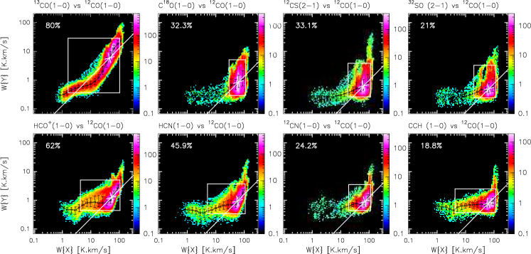
Figure 12: Joint distributions of various line intensities integrated over $[9,12\mathrm{\,km\,s^{-1}}]$. Markers have the same signification as in Fig. 10. The $x$-axis is always $W^{\mathrm{}}$$\left\{\mathrm{{}^{12}CO}\mathrm{(1-0)}\right\}$.

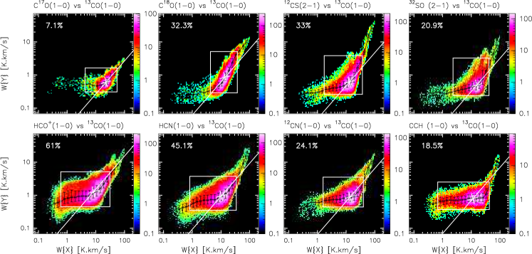
Figure 13: Same as Fig. 12, except that the $x$-axis is now $W^{\mathrm{}}$$\left\{\mathrm{{}^{13}CO}\mathrm{(1-0)}\right\}$.

Line intensity ratios are commonly used to study the physical and chemical properties of the gas in different environments. The advantage of using line ratios instead of absolute line intensities is that it allows to remove calibration uncertainties (when lines are observed simultaneously). It then is easier to compare from source to source. Line ratios may also remove excitation effects and bring forward actual chemical variations. Our knowledge of the chemistry of the gas then allows us to use line ratios to constrain the physical properties of the gas.

An important basic property we wish to determine easily from observations is the density of the gas. Forming dense gas is a required step to form stars, and the availability to form dense gas may regulate star formation efficiency (Lada et al., 2013). Line ratios of HCN and $\mathrm{HCO^{+}}$ with respect to $\mathrm{{}^{12}CO}$ and $\mathrm{{}^{13}CO}$ are commonly used to trace the fraction of dense gas in galactic and extragalactic GMCs (e.g., Lada et al., 2012). This is because $\mathrm{{}^{12}CO}$ and $\mathrm{{}^{13}CO}$ can be excited at low densities ($\sim 10^{2}\mathrm{\,cm^{-3}}$) compared to HCN and $\mathrm{HCO^{+}}$, which are expected to be excited only at high densities ($\sim 10^{5}\mathrm{\,cm^{-3}}$). Indeed, the HCN/$\mathrm{{}^{12}CO}$ ratio is observed to be well correlated with the star formation efficiency, traced by IR/HCN in M51 (e.g., Bigiel et al., 2016).

In this section we first show line ratios involving the brightest detected lines, i.e., $\mathrm{{}^{12}CO}$ and $\mathrm{{}^{13}CO}$ $\mathrm{(1-0)}$, and we conclude with a few other interesting ratios. For this, we discuss 2D-histograms of the ratio denominator vs. the ratio numerator, the spatial distribution of the ratios, and the 2D-histogram of the ratio vs. the visual extinction. This will allow us to study the correlations present before computing the ratio, to visually assess the correlations of the line ratios with different kinds of regions, and to quantitatively study potentially remaining correlations with the visual extinction.

6.1 Ratios with respect to $\mathrm{{}^{12}CO}$ and $\mathrm{{}^{13}CO}$ $\mathrm{(1-0)}$

The 2D-histograms shown in Fig. 12 display the relation of the integrated intensity of different lines as a function of the integrated intensity of the $\mathrm{{}^{12}CO}$ $\mathrm{(1-0)}$ line. While the eye is mainly caught by the saturation of the $\mathrm{{}^{12}CO}$ line, i.e., the fact that other tracer intensity increases by a large factor when $W^{\mathrm{}}(\mathrm{{}^{12}CO})\sim 100-200\mathrm{\,K\,km\,s^{-1}}$, most of the data follows a different trend. The running median and running interval containing 50% of the data, materialized as black points and error bars, indicate that most of the tracers have first a relatively constant integrated intensity as $W^{\mathrm{}}(\mathrm{{}^{12}CO})$ increases, and then their integrated intensity is well correlated to $W^{\mathrm{}}(\mathrm{{}^{12}CO})$. As shown by the white rectangles that display the part of the 2D-histogram populated by 90% of the points, most of the tracers only emit when the $\mathrm{{}^{12}CO}$ $\mathrm{(1-0)}$ line is already quite bright at $\sim 10-20\mathrm{\,K\,km\,s^{-1}}$. On the other hand, the CCH, $\mathrm{HCN}$, $\mathrm{HCO^{+}}$, and $\mathrm{{}^{13}CO}$ $\mathrm{(1-0)}$ lines show a significant fraction of the data at $\mathrm{{}^{12}CO}$ $\mathrm{(1-0)}$ integrated intensity between 1 and 10$\mathrm{\,K\,km\,s^{-1}}$. The $\mathrm{{}^{13}CO}$ $\mathrm{(1-0)}$ line has a specific behavior as it is under-luminous with respect to a linear correlation going through the median behavior at intermediate $\mathrm{{}^{12}CO}$ $\mathrm{(1-0)}$ intensities $(5\la W^{\mathrm{}}(\mathrm{{}^{12}CO})\la 30\mathrm{\,K\,km\,s^{-1}})$.

Figure 13 shows the same 2D-histograms as before but with respect to $W^{\mathrm{}}(\mathrm{{}^{13}CO})$. In general, the same trends seen for $\mathrm{{}^{12}CO}$ are seen for $\mathrm{{}^{13}CO}$. The species integrated intensities have a relatively constant or slightly increasing integrated intensity as $W^{\mathrm{}}(\mathrm{{}^{13}CO})$ increases up to $\sim 10\mathrm{\,K\,km\,s^{-1}}$. Their intensity is then well correlated to $W^{\mathrm{}}(\mathrm{{}^{13}CO})$. The effects of the $\mathrm{{}^{13}CO}$ $\mathrm{(1-0)}$ saturation are visible but less pronounced than with respect to the $\mathrm{{}^{12}CO}$ $\mathrm{(1-0)}$ line.

Figure 14 presents the spatial distribution of the line ratios involving $\mathrm{{}^{12}CO}$. The ratios are normalized by their median value to emphasize the symmetric departure of the ratios compared to the general trend. The ratios all show minimum values in the dense regions associated with NGC 2024, NGC 2023, and Horsehead. This probably reflects the saturation of the $\mathrm{{}^{12}CO}$ emission in regions with the highest column density. These regions are also the densest regions, which implies that the molecular tracers are easily produced and excited.

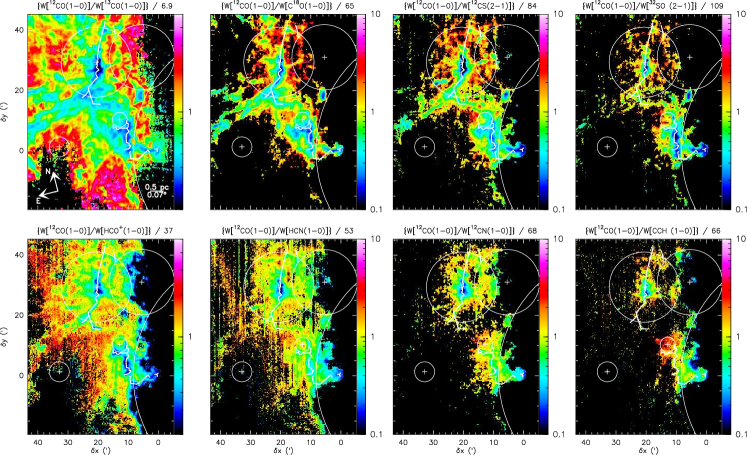
Figure 14: Spatial distribution of the ratios of line intensity integrated over $[9,12\mathrm{\,km\,s^{-1}}]$. The ratios are normalized by the median value of the ratio. The numerator is always $W^{\mathrm{}}$$\left\{\mathrm{{}^{12}CO}\mathrm{(1-0)}\right\}$. The color scale shows ratio values between 0.1 and 10 for all the ratio panels, except the $\mathrm{{}^{12}CO}$/$\mathrm{{}^{13}CO}$ and $\mathrm{{}^{12}CO}$/$\mathrm{HCO^{+}}$ panels where the color scale goes from 0.2 to 5.

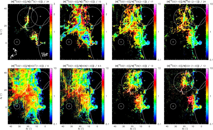
Figure 15: Same as Fig. 14, except that the numerator is now $W^{\mathrm{}}$$\left\{\mathrm{{}^{13}CO}\mathrm{(1-0)}\right\}$. The color scale shows ratio values between 0.1 and 10 for all the ratio panels, except the $\mathrm{{}^{13}CO}$/$\mathrm{C^{17}O}$ and $\mathrm{{}^{13}CO}$/$\mathrm{C^{17}O}$ panels where the color scale goes from 0.33 to 3.

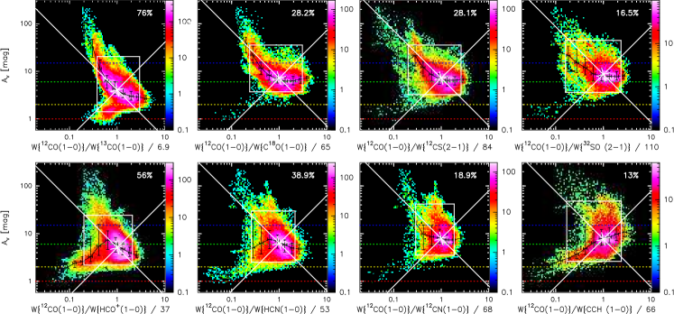
Figure 16: Joint distributions of the visual extinction as a function of the ratios of line integrated intensities. The ratios are normalized by their median value. The ratio numerator is always here $W^{\mathrm{}}$$\left\{\mathrm{{}^{12}CO}\mathrm{(1-0)}\right\}$. Markers have the same signification as in Fig. 10.

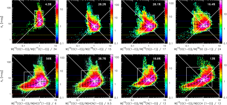
Figure 17: Same as Fig. 16, except that the ratio numerator is now $W^{\mathrm{}}$$\left\{\mathrm{{}^{13}CO}\mathrm{(1-0)}\right\}$.

As the $\mathrm{{}^{12}CO}$ line becomes saturated, the available energy gets carried away by other $\mathrm{{}^{12}CO}$ transitions or other molecular species. A West-East gradient is superimposed on the first pattern for the ratios involving $\mathrm{HCO^{+}}$, $\mathrm{HCN}$, $\mathrm{C_{2}H}$, $\mathrm{{}^{12}CN}$, and $\mathrm{HNC}$ (not shown), for both $\mathrm{{}^{12}CO}$ and $\mathrm{{}^{13}CO}$. The minimum values are obtained on the Western edge, the maximum values in the Eastern diffuse region. This pattern probably indicates a gradient in excitation and abundance in UV illuminated regions for molecules sensitive to the far-UV radiation. Finally an approximately circular structure around NGC 2024 with a luminosity deficit in $\mathrm{C^{18}O}$, $\mathrm{{}^{12}CS}$ and marginally $\mathrm{{}^{32}SO}$ probably traces UV illuminated material near NGC 2024.

Similar spatial behavior is also seen for the ratios with respect to $\mathrm{{}^{13}CO}$ $\mathrm{(1-0)}$ (see Fig. 15), but slightly attenuated because the saturation of the $\mathrm{{}^{13}CO}$ $\mathrm{(1-0)}$ line is less pronounced. The first pattern (minimum ratio values in regions of highest density) for the ratios including $\mathrm{C^{18}O}$, $\mathrm{{}^{12}CS}$, and $\mathrm{{}^{32}SO}$ supports the interpretation in terms of opacity for the densest/brightest regions. The East-West pattern is even more pronounced for the $\mathrm{HCO^{+}}$ species with an excess emission of the molecular tracers in the UV illuminated regions and a deficit in the diffuse/translucent gas. This may be a combined effect of lower heating, moderate density, and an increase of $\mathrm{{}^{13}CO}$ due to isotopic fractionation $(\mathrm{{}^{12}CO}+\mathrm{{}^{13}C^{+}}\longrightarrow\mathrm{{}^{13}CO}+\mathrm{{}^{12}C^{+}})$. Finally, the East-West pattern does not reach the translucent regions on the Eastern side for $\mathrm{C_{2}H}$, and CN. In these cases, we mostly see the increase of the line ratio in the high extinction gas, including the compressed Western edge (Schneider et al., 2013).

Finally, Fig. 16 shows the 2D-histograms of $A_{\mathrm{V}}^{\mathrm{}}$ as a function of the line ratios involving $\mathrm{{}^{12}CO}$. The line ratios have a bimodal behavior relative to $A_{\mathrm{V}}^{\mathrm{}}$, with values lower than the median (marked by the white cross) found both for high and low $A_{\mathrm{V}}^{\mathrm{}}$ regions. Values of the ratios higher than the median are associated with a small range of visual extinctions, either the translucent ($2<A_{\mathrm{V}}^{\mathrm{}}<6$) or filamentary ($6<A_{\mathrm{V}}^{\mathrm{}}<15$) gas. The bimodal trend is present in all ratios, but more pronounced for those involving lines presenting an extended emission ($\mathrm{{}^{13}CO}/\mathrm{{}^{12}CO}$ and $\mathrm{HCO^{+}}/\mathrm{{}^{12}CO}$).

The increasing branch (in $A_{\mathrm{V}}^{\mathrm{}}$) is the dominating one for the ratios involving $\mathrm{{}^{13}CO}$, $\mathrm{C^{18}O}$, $\mathrm{{}^{12}CS}$, $\mathrm{{}^{32}SO}$, and $\mathrm{{}^{12}CN}$. This means that the other decreasing branch, while existing, represents a small number of points in our field of view. Low values of these ratios thus mostly point to high density regions. The increasing branch is most likely a consequence of the saturation of the $\mathrm{{}^{12}CO}$ $\mathrm{(1-0)}$ line compared to the other lines at large gas column densities. In addition, many molecular species will become more abundant at large column densities, as they become shielded from UV-radiation. Both effects will produce lower ratios at large $A_{\mathrm{V}}^{\mathrm{}}$. Because all tracers are correlated to first order to the column density, one would expect to remove a correlation with $A_{\mathrm{V}}^{\mathrm{}}$ by taking the ratio of two lines. However, a (anti-)correlation may remain. This is due to the fact that the correlation between the integrated intensity of weaker lines and $W^{\mathrm{}}(\mathrm{{}^{12}CO})$ have a non-linear behavior, probably because these lines have a lower opacity than the $\mathrm{{}^{12}CO}$ $\mathrm{(1-0)}$ line for large gas column densities.

In contrast, the decreasing branch dominates for the ratios involving the $\mathrm{HCO^{+}}$, $\mathrm{HCN}$, and $\mathrm{C_{2}H}$ $\mathrm{(1-0)}$ lines. Low values of these ratios point to the lower visual extinction range. This is clear for $\mathrm{{}^{12}CO}/\mathrm{C_{2}H}$, whose running median almost monotonically increases from an $A_{\mathrm{V}}^{\mathrm{}}$ of $\sim 2$ to 10$\mathrm{\,mag}$. When the $\mathrm{{}^{12}CO}\mathrm{(1-0)}/\mathrm{HCO^{+}}\mathrm{(1-0)}$ and $\mathrm{{}^{12}CO}\mathrm{(1-0)}/\mathrm{HCN}\mathrm{(1-0)}$ ratios increase, the running median of the visual extinction first increases from values lower than $2\mathrm{\,mag}$ up to $\sim 8\mathrm{\,mag}$, and it then starts to decrease again. One interesting result is that all decreasing branches sample values of the visual extinction as low as $1-2\mathrm{\,mag}$. This is consistent with the fact that all the associated species are detected in diffuse clouds through absorption against extra-galactic continuum sources (Lucas & Liszt, 1996, 2000; Liszt & Lucas, 2001). This probably means that the strongly polar species, $\mathrm{C_{2}H}$, and $\mathrm{HCO^{+}}$, reach a radiative regime where they emit more efficiently than $\mathrm{{}^{12}CO}$, the weak excitation regime described by Liszt & Pety (2016).

Figure 17 shows the 2D-histograms of the visual extinction as a function of the ratio involving $\mathrm{{}^{13}CO}$. We see similar global results as for $\mathrm{{}^{12}CO}$, i.e., a globally constant visual extinction at values of the ratio higher than the median, and an increasing and a decreasing $A_{\mathrm{V}}^{\mathrm{}}$ branches when the ratio decreases below the median value. In contrast with the ratios involving $\mathrm{{}^{12}CO}$ $\mathrm{(1-0)}$, the decreasing $A_{\mathrm{V}}^{\mathrm{}}$ branch dominates for most of the ratios. Indeed, the running median for all ratios but $\mathrm{C^{18}O}/\mathrm{{}^{13}CO}$ decrease for low visual extinctions. The decrease is even almost monotonic for ratios involving the $\mathrm{HCO^{+}}$, $\mathrm{C_{2}H}$, $\mathrm{{}^{12}CN}$, and $\mathrm{HCN}$ $\mathrm{(1-0)}$ lines. This behavior is consistent with the fact that the correlation between the integrated intensity of the different species and $W^{\mathrm{}}(\mathrm{{}^{13}CO})$ is more linear. Taking the ratios thus better removes the correlations with the gas column density.

Table 10: Minimum, median, and maximum values of the ratios of diverse line integrated intensities.

Species #1	Trans.	Species #2	Trans.	$W^{\mathrm{}}(\#1)/W^{\mathrm{}}(\#2)$
				min$-$med$-$max
$\mathrm{{}^{12}CO}$	$1-0$	$\mathrm{{}^{13}CO}$	$1-0$	$1.2-6.9-46$
$\mathrm{{}^{12}CO}$	$1-0$	$\mathrm{HCO^{+}}$	$1-0$	$1.6-37-140$
$\mathrm{{}^{12}CO}$	$1-0$	$\mathrm{C^{18}O}$	$1-0$	$2.9-65-410$
$\mathrm{{}^{12}CO}$	$1-0$	$\mathrm{{}^{12}CN}$	$1-0$	$1.9-68-210$
$\mathrm{{}^{12}CO}$	$1-0$	$\mathrm{C_{2}H}$	$1-0$	$1.8-66-320$
$\mathrm{{}^{12}CO}$	$1-0$	$\mathrm{HNC}$	$1-0$	$1.8-66-320$
$\mathrm{{}^{12}CO}$	$1-0$	$\mathrm{{}^{12}CS}$	$2-1$	$2.4-84-350$
$\mathrm{{}^{12}CO}$	$1-0$	$\mathrm{{}^{32}SO}$	$2-1$	$2.7-110-400$
$\mathrm{{}^{13}CO}$	$1-0$	$\mathrm{HCO^{+}}$	$1-0$	$0.16-6-30$
$\mathrm{{}^{13}CO}$	$1-0$	$\mathrm{C_{2}H}$	$1-0$	$0.4-13-91$
$\mathrm{{}^{13}CO}$	$1-0$	$\mathrm{{}^{12}CN}$	$1-0$	$0.47-13-57$
$\mathrm{{}^{13}CO}$	$1-0$	$\mathrm{C^{18}O}$	$1-0$	$0.57-15-50$
$\mathrm{{}^{13}CO}$	$1-0$	$\mathrm{HNC}$	$1-0$	$0.4-13-91$
$\mathrm{{}^{13}CO}$	$1-0$	$\mathrm{{}^{12}CS}$	$2-1$	$0.71-17-70$
$\mathrm{{}^{13}CO}$	$1-0$	$\mathrm{{}^{32}SO}$	$2-1$	$0.67-24-98$
$\mathrm{{}^{13}CO}$	$1-0$	$\mathrm{C^{17}O}$	$1-0$	$0.65-34-85$
$\mathrm{HNC}$	$1-0$	$\mathrm{{}^{12}CN}$	$1-0$	$0.33-1.7-6.4$
$\mathrm{{}^{12}CS}$	$2-1$	$\mathrm{HNC}$	$1-0$	$0.22-1.1-7.3$
$\mathrm{{}^{12}CN}$	$1-0$	$\mathrm{HNC}$	$1-0$	$0.22-1.1-3.9$
$\mathrm{C^{18}O}$	$1-0$	$\mathrm{{}^{12}CS}$	$2-1$	$0.14-1.2-6.2$
$\mathrm{C^{18}O}$	$1-0$	$\mathrm{HNC}$	$1-0$	$0.16-1.3-8.5$
$\mathrm{HCN}$	$1-0$	$\mathrm{{}^{12}CN}$	$1-0$	$0.33-1.7-6.4$
$\mathrm{HCO^{+}}$	$1-0$	$\mathrm{HCN}$	$1-0$	$0.33-1.7-6.4$
$\mathrm{HCN}$	$1-0$	$\mathrm{HNC}$	$1-0$	$0.33-1.7-6.4$
$\mathrm{HCO^{+}}$	$1-0$	$\mathrm{HNC}$	$1-0$	$0.33-1.7-6.4$
$\mathrm{C^{18}O}$	$1-0$	$\mathrm{C^{17}O}$	$1-0$	$0.43-4.3-8.6$
$\mathrm{HCO^{+}}$	$1-0$	$\mathrm{N_{2}H^{+}}$	$1-0$	$0.33-1.7-6.4$

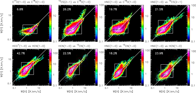
Figure 18: Same as Fig. 12, except that there is no common $x$-axis in this figure.

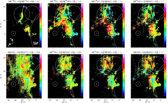
Figure 19: Same as Fig. 14, except that there is no common numerator in this figure.

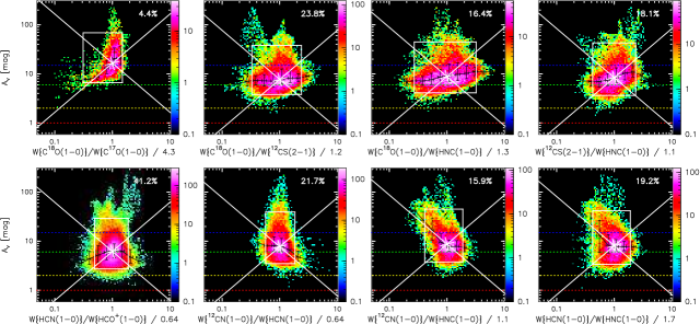
Figure 20: Same as Fig. 14, except that there is no common ratio numerator in this figure.

6.2 Various other line ratios

Figure 18 to 20 show the same plots as the previous section but for other line ratios including tracers of the column density ($\mathrm{C^{18}O}$, $\mathrm{{}^{12}CS}$, and $\mathrm{HNC}$), and other highly studied ratios in extra-galactic observations ($\mathrm{HCO^{+}}$, $\mathrm{HCN}$, $\mathrm{HNC}$, and CN).

The 2D-histograms that display the relation of the integrated intensity of $\mathrm{C^{17}O}$, $\mathrm{HNC}$, and $\mathrm{{}^{12}CS}$ with respect to $W^{\mathrm{}}(\mathrm{C^{18}O})$ show two main behaviors (see Fig. 19). The $\mathrm{C^{17}O}$, $\mathrm{HNC}$, and $\mathrm{{}^{12}CS}$ $\mathrm{(2-1)}$ lines are over-luminous compared to the $\mathrm{C^{18}O}$ $\mathrm{(1-0)}$ line at low intensities. Their intensities then become linearly correlated. In addition, the $\mathrm{{}^{12}CS}$ $\mathrm{(2-1)}$ line becomes much brighter than both the $\mathrm{C^{18}O}$ and $\mathrm{HNC}$ $\mathrm{(1-0)}$ lines at high intensity values. The integrated brigthnesses of the HCN-$\mathrm{HCO^{+}}$, $\mathrm{HNC}$-$\mathrm{HCO^{+}}$, $\mathrm{HNC}$-$\mathrm{CN}$, and HNC-HCN $\mathrm{(1-0)}$ line pairs are all linearly correlated. The best correlation is found for the $\mathrm{HCN}$-$\mathrm{CN}$ pair of lines.

The spatial patterns of the ratios shown in Fig. 19 are less obvious to describe because the fraction over the field of view where the two lines are detected at enough signal-to-noise ratio is lower. The $\mathrm{C^{18}O}/\mathrm{C^{17}O}$ ratio, shown in the upper left panel, is fairly flat with no clear spatial pattern. The East-West pattern is particularly marked on the $\mathrm{C^{18}O}/\mathrm{{}^{12}CS}$ and $\mathrm{HNC}/\mathrm{C^{18}O}$ ratios. The $\mathrm{{}^{12}CS}/\mathrm{HNC}$, $\mathrm{{}^{12}CN}/\mathrm{HNC}$, and $\mathrm{HCN}/\mathrm{HNC}$ ratios all show an approximately circular structure around NGC 2024 with a deficit of $\mathrm{HNC}$ integrated intensity. We relate the latter behavior to an isomerisation of $\mathrm{HNC}$ into $\mathrm{HCN}$ when the gas temperature increases.

Computing the ratio for these lines removed almost any linear (anti-)correlation with the visual extinction, except for the $\mathrm{HCN}/\mathrm{HNC}$ and $\mathrm{CN}/\mathrm{HNC}$ ratios (see Fig. 20). For the filamentary gas ($A_{\mathrm{V}}^{\mathrm{}}$ between 6 and 15$\mathrm{\,mag}$) the ratio spans a large range of values, up to one order of magnitude for $\mathrm{C^{18}O}/\mathrm{{}^{12}CS}$ and $\mathrm{C^{18}O}/\mathrm{HNC}$.

7 Discussion

7.1 Typical line intensities in a strongly UV illuminated part of a GMC

Table 11: Visual extinction, dust temperature, and far UV illumination for three different regions of 1 square-degree area in Orion B.

Environment	$A_{\mathrm{V}}^{\mathrm{min}}-A_{\mathrm{V}}^{\mathrm{5\%}}-A_{\mathrm{V}}^{\mathrm{med}}-A_{\mathrm{V}}^{\mathrm{95\%}}-A_{\mathrm{V}}^{\mathrm{max}}$	$T_{\mathrm{d}}^{\mathrm{min}}-T_{\mathrm{d}}^{\mathrm{5\%}}-T_{\mathrm{d}}^{\mathrm{med}}-T_{\mathrm{d}}^{\mathrm{95\%}}-T_{\mathrm{d}}^{\mathrm{max}}$	$G_{0}^{\mathrm{min}}-G_{0}^{\mathrm{5\%}}-G_{0}^{\mathrm{med}}-G_{0}^{\mathrm{95\%}}-G_{0}^{\mathrm{max}}$
	$\mathrm{\,mag}$	$\mathrm{\,K}$	ISRF (Habing, 1968)
UV illuminated	$0.76-1-3.3-12-230$	$16.4-20.1-24.1-40.5-101$	$4.4-12-30-400-38000$
Translucent	$1.1-1.5-2.4-3.5-7.7$	$16-17.2-17.9-18.6-20.3$	$3.9-5.6-6.9-8.1-13$
UV shieded	$1.5-2.2-3.4-7.9-34$	$12.9-15.2-17.1-18.5-20.3$	$1.3-3-5.3-8-13$

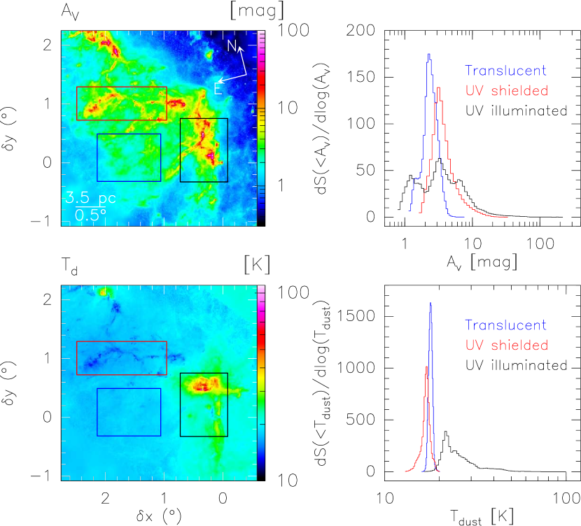
Figure 21: Left panels: Spatial distribution of the visual extinction and of the dust temperature. Right panels: Probability distribution functions of the visual extinction and the dust temperature for the regions inside the black, blue, and red rectangles, respectively.

The field of view sampled here is not a random 1 square degree part of any GMC. The left panels of Fig. 21 show the spatial distribution of the visual extinction and dust temperature over a much larger fraction of the Orion B molecular cloud than the one presented in this paper, which is shown as the black rectangle. The right panels compare the Probability Distribution Functions (PDFs) of dust properties over our field of view with the PDFs of two other regions with same surface area. Table 11 lists the minimum, median, and maximum values of the associated distributions, as well as their 5 and 95% quantiles. This clearly shows that three different kinds of environment exist in the Orion B molecular cloud. First, the lowest dust temperatures are associated with relatively high visual extinctions (red rectangle). Second, the blue rectangle identifies a translucent region (all pixels have $A_{\mathrm{V}}^{\mathrm{}}\la 8$), associated with a typical dust temperature of about 18$\mathrm{\,K}$. In both cases, the distribution of visual extinction and dust temperature are single peaked with a narrow full width at half maximum. In contrast, our field of view displays wide $A_{\mathrm{V}}^{\mathrm{}}$ and $T_{\mathrm{d}}^{\mathrm{}}$ distributions, and it is associated with the highest dust temperatures with a median value of $\sim 24\mathrm{\,K}$ $(G_{0}^{\mathrm{}}\sim 30)$. The presence of high gas temperatures is confirmed by the large $\mathrm{{}^{12}CO}$ $\mathrm{(1-0)}$ peak temperatures that are lower limits of the kinetic temperature (Orkisz et al., subm.). These properties are associated with the presence of at least four H ii regions (see Section 2.1) that imply a large UV illumination (see the fourth column of Table 11). In particular, the minimum dust temperature in our field (16.4$\mathrm{\,K}$) is rather high in Orion B compared to the Taurus molecular cloud (Marsh et al., 2014).

Table 4 indicates that, under these sampling conditions and at the typical sensitivity achieved in studies of nearby galaxies ($3\sigma=1\mathrm{\,K\,km\,s^{-1}}$), only the $\mathrm{(1-0)}$ line of $\mathrm{{}^{12}CO}$, $\mathrm{{}^{13}CO}$, $\mathrm{HCO^{+}}$, $\mathrm{HCN}$ would easily be detected by a single-dish radio-telescope of 30m-diameter with a single-beam receiver. A 10 times better sensitivity (100 longer integration) is required to detect the $\mathrm{(1-0)}$ or $\mathrm{(2-1)}$ lines of HCN, CN, $\mathrm{C^{18}O}$, $\mathrm{{}^{12}CS}$, $\mathrm{C_{2}H}$, $\mathrm{HNC}$, $\mathrm{{}^{32}SO}$, $\mathrm{C^{17}O}$, and $\mathrm{c-C_{3}H_{2}}$. Finally, another order-of-magnitude increase of the sensitivity ($3\sigma=0.01\mathrm{\,K\,km\,s^{-1}}$) would be needed to detect $\mathrm{N_{2}H^{+}}$, $\mathrm{CH_{3}OH}$, $\mathrm{H^{13}CO^{+}}$, and $\mathrm{H^{13}CN}$. This means that detecting rare isotopologues of $\mathrm{HCO^{+}}$, $\mathrm{HCN}$, or $\mathrm{HNC}$ in nearby galaxies is difficult to achieve with a single-dish radio-telescope because of the dilution of the signal in the beam.

7.2 On the influence of the UV field on the determination of molecular mass

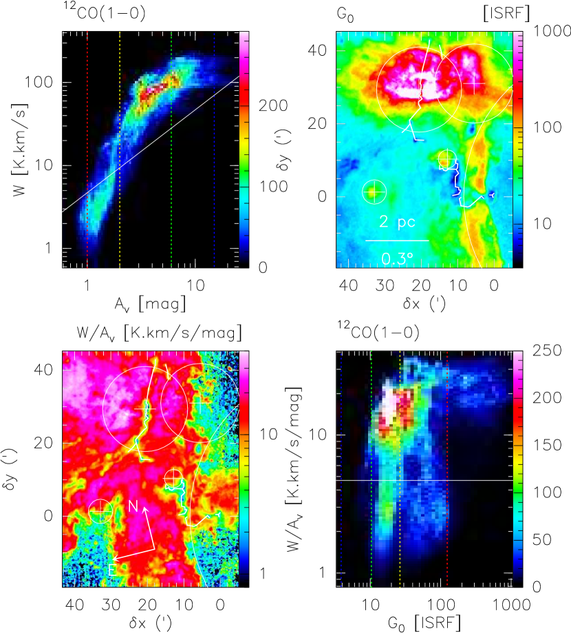
Figure 22: Top, left panel: Joint distribution of the $\mathrm{{}^{12}CO}$ $\mathrm{(1-0)}$ line integrated intensity as a function of the visual extinction. The number of sightlines falling in a given 2D bin of the distribution is color-coded using a linear scale to emphasize the bi-modal nature of the distribution. The white line shows the location of points that follows $N(\mathrm{H_{2}})=X_{\mathrm{CO}}\,W^{\mathrm{}}$. The red, orange, green, and blue vertical dashed lines show the visual extinction limits (1, 2, 6, and 15 magnitudes, respectively) used in the masks of Fig. 6. Top, right panel: Spatial distribution of the far UV illumination in units of the ISRF (Habing, 1968). Bottom, left panel: Ratio of the $\mathrm{{}^{12}CO}$ $\mathrm{(1-0)}$ line integrated intensity to the visual extinction. Bottom, right panel: Joint distribution of this ratio as a function of the far UV illumination. The horizontal white line corresponds to the standard value of the $X_{\mathrm{CO}}$ factor. The blue, green, orange, and red vertical dashed lines show the far UV illumination limits (4, 10, 26, and 120, respectively), which corresponds to the dust temperature limits used in the masks of Fig. 8. The color scales of the two images show the same ranges as the axes of the bottom right joint distribution.

The average visual extinction and CO integrated intensity for the observed field of view are 4.7$\mathrm{\,mag}$ and 61$\mathrm{\,K\,km\,s^{-1}}$. This turns into a $W^{\mathrm{}}_{\mathrm{CO}}/A_{\mathrm{V}}^{\mathrm{}}=13.0\mathrm{\,K\,km\,s^{-1}}/\mathrm{\,mag}$, while the standard $X_{\mathrm{CO}}$ factor, i.e., $2\times 10^{20}\,\mathrm{H_{2}}\mathrm{\,cm^{-2}}/(\mathrm{\,K\,km\,s^{-1}})$, corresponds to $4.7\mathrm{\,K\,km\,s^{-1}}/\mathrm{\,mag}$ when we assume a standard $N_{\mathrm{H}}/A_{\mathrm{V}}^{\mathrm{}}$ factor and fully molecular gas. The H i emission indicates that diffuse gas accounts for about 1 magnitude of extinction towards Orion B (see Section 3.4). Assuming that contribution from atomic hydrogen to the mass is negligible towards the mapped field of view overestimates the dust-traced molecular mass by 27%, increasing the discrepancy between the CO and dust-traced mass. Therefore, we neglect this subtlety and we directly compare the CO and dust-traced mass. We find that the CO-traced mass (and thus the associated surface and volume density) is about 3 times higher than the dust-traced mass.

The origin of this discrepancy lies in the intense UV illumination of the gas by massive stars. The bottom left panel of Fig. 22 compares the spatial distribution of the CO integrated intensity per visual extinction. The standard value of 4.7$\mathrm{\,K\,km\,s^{-1}}$/$\mathrm{\,mag}$ corresponds to the transition between yellow and green. Only diffuse gas or the UV shielded dense gas have $X_{\mathrm{CO}}$ values close or lower than standard. This is confirmed by the joint distribution of the $W^{\mathrm{}}_{\mathrm{CO}}$ and $A_{\mathrm{V}}^{\mathrm{}}$ where most of the points (lines of sight with $2\la A_{\mathrm{V}}^{\mathrm{}}\la 15$) lie above the white line of slope 4.7$\mathrm{\,K\,km\,s^{-1}}$/$\mathrm{\,mag}$. When the visual extinction increases, the CO intensity saturates. At the lowest visual extinction ($A_{\mathrm{V}}^{\mathrm{}}\la 2$), CO is destroyed into $\mathrm{C^{+}}$. The spatial distribution of $G_{0}^{\mathrm{}}$ clearly shows that most of the gas lies in regions with $G_{0}^{\mathrm{}}>10$, the mean value of $G_{0}^{\mathrm{}}$ being 45. Under such conditions, dust and gas are heated to higher temperature than in the standard interstellar radiation field. In the physical conditions of Orion B, the CO emission per $\mathrm{H_{2}}$ molecule is increasing with the kinetic temperature, leading to a possible bias in the mass determination. The bottom right panel of Fig. 22 shows that the CO intensity per $A_{\mathrm{V}}^{\mathrm{}}$ increases with $G_{0}^{\mathrm{}}$.

While it is tempting to conclude that only the CO traced mass is widely overestimated in such conditions, the dust-traced mass is in fact also underestimated, as indicated by the range of virial mass that we estimated from the field of view size and CO linewidth (see Table 2). It is known that using a single dust temperature to fit the spectral energy distribution on a line of sight that contains dust at different temperatures hides the presence of cold dust along the line of sight, because the luminosity of dust increases extremely fast with its temperature (Shetty et al., 2009).

All in all, the typical volume density we infer for the regions, i.e., between 200 and $600\,\mathrm{H_{2}}\mathrm{\,cm^{-3}}$, is typical of galactic Giant Molecular Clouds (Heyer & Dame, 2015). While the local values of $N_{\mathrm{H}}/A_{\mathrm{V}}^{\mathrm{}}$ and $X_{\mathrm{CO}}$ are uncertain, and they could well be different from their standard values in Orion B, we here wish to study Orion B as if it was observed from nearby galaxies. In these studies, standard values are used when the metallicity is similar to that of the Milky Way (e.g., see the PAWS project Schinnerer et al., 2013; Pety et al., 2013). From a practical viewpoint, we thus proceeded with standard values, knowing that the correct result is probably in between the CO-traced and dust-traced masses, surface densities, and volume densities.

Enhanced far UV fields heat large masses of CO gas that turns over-luminous with respect to the standard $X_{\mathrm{CO}}$ factor, i.e., the average behavior of the CO gas in our Milky way (Planck Collaboration et al., 2011b). This effect could compensate for the presence of CO-dark gas (Wolfire et al., 2010; Planck Collaboration et al., 2015), as proposed by Liszt & Pety (2012) with different observations. Therefore the standard value of $X_{\mathrm{CO}}$ may well be applicable to galaxies with a higher than average, yet moderate, massive star formation rate. An easy check would be to increase the size of the mapped field of view to the full Orion B cloud to test at which scale the CO and dust-traced masses derived with standard values of $X_{\mathrm{CO}}$ and the $N_{\mathrm{H}}$/$A_{\mathrm{V}}^{\mathrm{}}$ ratio get reconciled to better than a factor 3. Complementary Cii observations would also help to settle this point (Goicoechea et al., 2015).

Table 12: Critical density, and percentage of total flux originating from gas in filaments and dense cores for each line.

Species	Transition	$n_{\mathrm{crit}}{}$	$F_{6\leq A_{\mathrm{V}}^{\mathrm{}}<15}$	$F_{15\leq A_{\mathrm{V}}^{\mathrm{}}}$
		$\mathrm{\,cm^{-3}}$	% of $F_{\mathrm{tot}}$	% of $F_{\mathrm{tot}}$
$\mathrm{{}^{12}CO}$	$1-0$	$2\times 10^{3}$	$38$	$7.6$
$\mathrm{{}^{13}CO}$	$1-0$	$2\times 10^{3}$	$45$	$15$
$\mathrm{HCO^{+}}$	$1-0$	$2\times 10^{5}$	$40$	$16$
$\mathrm{C_{2}H}$	$1-0$	$1\times 10^{5}$	$37$	$17$
$\mathrm{c-C_{3}H_{2}}$	$2-1$	$1\times 10^{6}$	$38$	$17$
$\mathrm{HCN}$	$1-0$	$3\times 10^{6}$	$44$	$18$
$\mathrm{{}^{12}CN}$	$1-0$	$3\times 10^{5}$	$45$	$19$
$\mathrm{C^{17}O}$	$1-0$	$2\times 10^{3}$	$43$	$26$
$\mathrm{HNC}$	$1-0$	$4\times 10^{5}$	$41$	$27$
$\mathrm{C^{18}O}$	$1-0$	$2\times 10^{3}$	$48$	$29$
$\mathrm{{}^{32}SO}$	$2-1$	$2\times 10^{5}$	$44$	$31$
$\mathrm{{}^{12}CS}$	$2-1$	$2\times 10^{5}$	$42$	$32$
$\mathrm{CH_{3}OH}$	$2-1$	$3\times 10^{4}$	$41$	$48$
$\mathrm{H^{13}CO^{+}}$	$1-0$	$2\times 10^{5}$	$34$	$56$
$\mathrm{N_{2}H^{+}}$	$1-0$	$2\times 10^{5}$	$17$	$88$

Table 13: Flux ratios in nearby galaxies and in Orion B.

Source	HCN/$\mathrm{HCO^{+}}$	$\mathrm{{}^{12}CO}$/HCN	$\mathrm{{}^{12}CO}$/$\mathrm{HCO^{+}}$	$\mathrm{{}^{12}CO}$/$\mathrm{N_{2}H^{+}}$	$\mathrm{{}^{12}CN}$/HCN	$\mathrm{C_{2}H}$/$\mathrm{{}^{13}CO}$	HCN/HNC	Observ.	Ref.
ULIRGs	$1.5-2.4$	$6.3-8.6$	$9.7-21$	$40$	$0.4-0.5$	$0.8-1.4$	$1.4-3.0$	MOPRA-22m	1
M51 P2	$1.2$	$32$	$39$	$225$	$0.5$	$0.04$	$2.7$	IRAM-30m	2
AGNs	$0.8-2.0$	$3.4-25$	$5.7-20$	$41-68$	$0.9-1.6$	$0.2-0.7$	$2.2-3.0$	IRAM-30m	3
Starbursts	$0.7-1.2$	$16-23$	$16-24$	$100-325$	$1.2-1.4$	$0.2-0.7$	$1.9-2.5$	IRAM-30m	3
M82	$0.5$	-	-	-	-	-	-	CARMA	4
NGC253 P7	$1.2$	$6.0$	$7.0$	-	$0.6$	-	-	ALMA	5
Maffei2B	$0.6$	-	-	-	-	-	$4.3$	BIMA,OVRO	6
LMC	$0.4-0.7$	$11-120$	$6.0-48$	$59-167$	$0.2-0.3$	$0.03-0.27$	$1.1-3.4$	IRAM-30m	7
OrionB	$0.9$	$39$	$37$	$900$	$0.5$	$0.05$	$3.5$	IRAM-30m	8

7.3 Dense gas tracers

The brightness of a molecular line depends on the column density of the species, which is affected by the chemistry, and the excitation properties of the line. These in turn depend on the physical properties of the gas (density, temperature, ionization fraction, …). Indeed, two conditions must be satisfied for a line to be detected. First, the molecule has to abundant enough, and second, the excitation conditions must be favorable for the line to be excited and produce bright line emission. It is therefore often assumed that lines with high critical densities, such as the $\mathrm{(1-0)}$ lines of HCN and $\mathrm{HCO^{+}}$, are good tracers of dense gas because these species are abundant and their emission is expected to be seen only in regions where the density is high enough to excite the line. Table 10 lists the critical density of each molecular line as well as the percentage of total flux that is emitted from regions of intermediate $(6\leq A_{\mathrm{V}}^{\mathrm{}}<15)$ and high $(15\leq A_{\mathrm{V}}^{\mathrm{}})$ visual extinction, as measured in Section 4.1. These two regimes are representative of the gas arising in filaments and dense cores, respectively. We do not find any clear correlation between the critical density of the lines and the percentage of flux emitted.

For instance, the lines of the CO isotopologues have nearly equal critical densities (i.e., similar excitation conditions) but the percentage of flux coming from the densest regions $(n_{\mathrm{H_{2}}}\sim 7\,300\mathrm{\,cm^{-3}})$ varies from 8% for $\mathrm{{}^{12}CO}$ $\mathrm{(1-0)}$ to 29% for $\mathrm{C^{18}O}$ $\mathrm{(1-0)}$. The higher fraction of flux coming from high density regions for the rarer isotopologues is the result of both sensitivity and chemistry. The intrinsic lower abundance of $\mathrm{{}^{13}CO}$, $\mathrm{C^{18}O}$ and $\mathrm{C^{17}O}$ compared to the main isotope will result in weaker emission for the rarer isotopologues everywhere in the cloud. Also, in the UV-illuminated layers $\mathrm{{}^{12}CO}$ will survive longer than the CO isotopologues due its capacity to self-shield (process known as selective photo dissociation), although this effect is probably not resolved by the observations.

Lines with much higher critical densities ($>10^{5}\mathrm{\,cm^{-3}}$) than CO $\mathrm{(1-0)}$ ($\sim 10^{3}\mathrm{\,cm^{-3}}$), such as $\mathrm{HCO^{+}}$, $\mathrm{HCN}$, and $\mathrm{HNC}$ $\mathrm{(1-0)}$, which are expected to trace dense gas, emit only 16, 18, and 27% of their total flux in mapped Orion B regions of high density. Most of the emission then arises in lower density gas. Shirley (2015) extensively discusses the relevance of the notion of critical density. He reminds that the critical density is the density at which collisional deexcitation equals the net radiative emission. He emphasizes that it is computed in the optically thin limit, implying that it is only an upper limit in the presence of photon-trapping. The fact that these lines can be excited and thus detected in diffuse gas was in addition recently discussed by Liszt & Pety (2016). While their results can not be quantitatively applied to the observed field of view because the line peak intensities are slightly outside the range of applicability of the weak excitation regime, the underlying physical process is still present. At the limit of detectability, Liszt & Pety (2016) showed that the intensity of low-energy rotational lines of strongly polar molecules, such as $\mathrm{HCO^{+}}$ and $\mathrm{HNC}$, is proportional to the product of the total gas density and the molecule column density, independent of the critical density, as long as the line intensity does not increase above a given value. This implies that for any given gas density there is a column density that will produce an observable line intensity. In the observed field of Orion B, we are in an intermediate radiative transfer regime where the fundamental lines of $\mathrm{HCO^{+}}$, $\mathrm{HCN}$, and $\mathrm{HNC}$ can be excited in regions of density much smaller than their critical densities.

The lines with the largest fraction of their emission arising in the densest gas are $\mathrm{CH_{3}OH}$ and $\mathrm{N_{2}H^{+}}$. In particular, $\mathrm{N_{2}H^{+}}$ $\mathrm{(1-0)}$ that presents a similarly high critical density as $\mathrm{HCO^{+}}$, $\mathrm{HCN}$, and $\mathrm{HNC}$ $\mathrm{(1-0)}$, has the highest proportion of its flux coming from the densest regions (88%). Moreover, in contrast to all the other lines, only 17% of the total $\mathrm{N_{2}H^{+}}$ $\mathrm{(1-0)}$ flux is associated with regions of intermediate $A_{\mathrm{V}}^{\mathrm{}}$ ($6\leq A_{\mathrm{V}}^{\mathrm{}}<15$) which have typical densities of $\sim 1\,500\mathrm{\,cm^{-3}}$. This shows that the $\mathrm{N_{2}H^{+}}$ $\mathrm{(1-0)}$ line is the best molecular tracer of dense regions among the lines studied in this paper.

Despite the similar critical densities between $\mathrm{N_{2}H^{+}}$ and $\mathrm{HCO^{+}}$, their behavior is completely different. First, $\mathrm{N_{2}H^{+}}$ is detected over only 2.4% of the observed field of view, while $\mathrm{HCO^{+}}$ emission covers 68% of the field. Second, the percentages of the flux coming from dense/translucent regions are 88/8% for $\mathrm{N_{2}H^{+}}$, and 15/41% for $\mathrm{HCO^{+}}$. These differences can only be understood by their different chemistry. $\mathrm{HCO^{+}}$ can be formed from ion-molecule reactions involving C⁺ and other cations, notably CH${}^{+}_{2}$ and CH${}^{+}_{3}$, in addition to the protonation of CO. On the contrary, the sole reaction producing $\mathrm{N_{2}H^{+}}$ is the protonation of $\mathrm{N_{2}}$. Furthermore, the destruction of $\mathrm{HCO^{+}}$ by dissociative recombination with electrons produces CO while $\mathrm{N_{2}H^{+}}$ can react with CO to produce $\mathrm{HCO^{+}}$. Hence, $\mathrm{N_{2}H^{+}}$ only survives in regions where the electron abundance is low (to prevent dissociative recombination) and where CO is frozen on dust grains (to prevent proton transfer to CO), i.e., in cold and dense cores.

In summary, species that have a chemical reason to only be present in dense gas are the only really reliable high density tracers. More generally, the knowledge of the chemical behavior is fundamental in understanding how molecular species can be used to trace the different physical environments.

7.4 Typical line ratios in Orion B and other galaxies

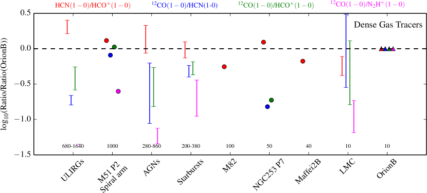
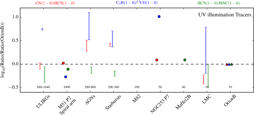
Figure 23: Line ratios observed towards nearby galaxies and the Orion B molecular cloud. The upper and lower panels include line ratios which are proposed dense gas and UV-illumination tracers, respectively. A point is plotted for individual measures, while a range of values is given for the ULIRG, AGN, and starburst samples, which contain measures for several galaxies. The ULIRGs include Arp 220 and Mrk 231, while AGNs include M51, NGC 1068 and NGC 7469, and the starburst galaxies include M83, NGC 253 and M82. The sources are sorted by decreasing spatial resolution, which is given at the bottom of the figure for each source. The Orion B values correspond to the ratios of the lines integrated over the full region to simulate a 10$\mathrm{\,pc}$ spatial resolution allowing a better comparison with the other galaxies.

Molecular line ratios have the potential to be powerful probes of physical properties related to star formation activity. Thanks to the current observing capabilities, many unbiased line surveys have recently been made towards nearby galaxies, and more than 27 species have been detected in the 3$\mathrm{\,mm}$ band (Meier & Turner, 2012; Salas et al., 2014; Watanabe et al., 2014; Aladro et al., 2015; Meier et al., 2015; Nishimura et al., 2016). Common line ratios include the $\mathrm{HCN}$$\mathrm{(1-0)}$/$\mathrm{HCO^{+}}$$\mathrm{(1-0)}$, $\mathrm{{}^{12}CO}$$\mathrm{(1-0)}$/$\mathrm{HCN}$$\mathrm{(1-0)}$, $\mathrm{HCN}$$\mathrm{(1-0)}$/$\mathrm{HNC}$$\mathrm{(1-0)}$ and the CN$\mathrm{(1-0)}$/$\mathrm{HCN}$$\mathrm{(1-0)}$, which are proposed tracers of density, temperature and radiation field, respectively.

Figure 23 shows observed line ratios in nearby galaxies and in the Orion B molecular cloud. The comparison includes line ratios obtained with both single-dish telescopes and interferometers, and galaxies with distances between 3.3 and 170$\mathrm{\,Mpc}$, in addition to the LMC, the nearest external galaxy (50$\mathrm{\,kpc}$). The sample therefore spans two orders of magnitude in spatial resolution (written at the bottom of the y-axis in units of pc). To ease the comparison with Orion B, the ratios are normalized by the Orion B ratios of the lines integrated over the full observed field of view (i.e., at a resolution of 10$\mathrm{\,pc}$).

Line ratios observed in Orion B are, in general, comparable to what is observed in nearby galaxies. Noticeably, line ratios (except $\mathrm{{}^{12}CO}$/$\mathrm{N_{2}H^{+}}$) in Orion B at a resolution of 10$\mathrm{\,pc}$ are very similar to those observed at a resolution of 1000$\mathrm{\,pc}$ in the spiral arm of the famous whirlpool galaxy (M 51), a prototype of grand design spiral galaxy.

The $\mathrm{HCN}$/$\mathrm{HCO^{+}}$ ratio (shown in red in the upper panel) is assumed to trace dense gas that will eventually form stars, and thus is often used to trace the star formation activity in other galaxies. Both lines are among the brightest lines observed and are thus easily detected. ULIRGs and AGNs present the largest $\mathrm{HCN}$/$\mathrm{HCO^{+}}$ ratios, but there are no major differences between the sources. The resolved spatial distribution in Orion B (see Fig. 19) shows that in the case of UV-illuminated gas, the $\mathrm{HCN}$/$\mathrm{HCO^{+}}$ ratio does not trace the high density gas. Another proposed tracer of dense gas is the inverse of the $\mathrm{{}^{12}CO}$/HCN ratio (shown in blue in the upper panel). This ratio is higher in Orion B, the LMC and in the spiral arm of M51 than in the other galaxies. The $\mathrm{{}^{12}CO}$/$\mathrm{HCO^{+}}$ ratio behaves in a similar way. While the resolved spatial distribution in Orion B (see Fig. 14) shows that these ratios actually separate diffuse from dense gas, the quantitative analysis shows that $\mathrm{HCO^{+}}$ and $\mathrm{HCN}$ $\mathrm{(1-0)}$ fluxes mostly trace densities around $500-1500\,\mathrm{H_{2}}\mathrm{\,cm^{-3}}$ instead of $\sim 10^{4}\mathrm{\,cm^{-3}}$.

Better tracers of high-density gas are ratios involving $\mathrm{N_{2}H^{+}}$, such as CO$\mathrm{(1-0)}$/$\mathrm{N_{2}H^{+}}$$\mathrm{(1-0)}$ (shown in magenta), because $\mathrm{N_{2}H^{+}}$ resides solely in dense gas ($>10^{4}\mathrm{\,cm^{-3}}$), contrary to $\mathrm{HCN}$ that can be present at lower densities (see Section 4.1). Starbursts (including M 51) and ULIRGs forms many stars, requiring the presence of many dense cores, and thus a high $\mathrm{N_{2}H^{+}}$ $\mathrm{(1-0)}$ brightness relative to $\mathrm{{}^{12}CO}$ $\mathrm{(1-0)}$ that traces the total reservoir of molecular gas. In contrast, Orion B has a low star formation efficiency (Lada et al., 2010; Megeath et al., 2016), probably implying a low number of dense cores and thus a lower relative $\mathrm{N_{2}H^{+}}$ brightness. The low surface filling factor of $\mathrm{N_{2}H^{+}}$ makes it difficult to detect at high signal-to-noise ratio with single-dish telescopes in external galaxies. Fortunately, the much better resolving power of NOEMA and ALMA relieves this difficulty and $\mathrm{N_{2}H^{+}}$ starts to be detected in nearby galaxies.

The $\mathrm{HCN}$/$\mathrm{HNC}$ is another popular line ratio measured in nearby galaxies (shown in green in the bottom panel). Both species are abundant in cold clouds, but at temperatures higher than about 30$\mathrm{\,K}$, $\mathrm{HNC}$ starts to be converted to $\mathrm{HCN}$ through reactions with H (see, e.g., Schilke et al., 1992; Graninger et al., 2014). The HCN/HNC ratio is thus increasing at higher temperatures. The sources included in this comparison present similar HCN/HNC ratios within a factor of 2. The spatial distribution shown in Fig. 19 is consistent with the proposed temperature dependence of this ratio, whose lowest values are found in the cold filaments, and which correlates well with the map of the dust temperature seen in Fig. 2.

Finally, the CN/HCN intensity ratio (shown in red in the bottom panel) is expected to trace UV-illuminated gas because CN is a major product of HCN photodissociation. Indeed, higher abundance ratios are found in PDRs and XDRs compared to cold dark clouds (Fuente et al., 2005; Baan et al., 2008). However, in spatially resolved observations, there is no clear correlation of the CN/HCN flux ratio with radiation field (see Fig. 19). Furthermore, in our comparison, AGNs and starbursts present the largest CN/HCN ratios, and ULIRGs have similar ratios to the Orion B cloud and the spiral arm of M51. This is contradictory with CN/HCN being a radiation field tracer. In fact, the ratios that involve the HCN $\mathrm{(1-0)}$ line must be taken with care because this line is known to be pumped by IR photons (Aalto et al., 2007). This will produce brighter HCN lines, and thus could explain the low CN/HCN ratio observed in ULIRGs. A better tracer of radiation field is the $\mathrm{C_{2}H}$$\mathrm{(1-0)}$/$\mathrm{{}^{13}CO}$$\mathrm{(1-0)}$ ratio. Carbon chains, such as $\mathrm{C_{2}H}$ and $\mathrm{C_{3}H_{2}}$, have been observed to form efficiently in UV-illuminated regions (Pety et al., 2005; Guzmán et al., 2015). ULIRGs, AGNs and starburst galaxies present the largest $\mathrm{C_{2}H}$/$\mathrm{{}^{13}CO}$ ratios, consistent with their high star formation activities. Moreover, the spatial distribution of the $\mathrm{C_{2}H}$/$\mathrm{{}^{13}CO}$ ratio (see Fig. 15) shows a clear gradient between the illuminated edge (right) and the UV-shielded (left) side of the Orion B molecular cloud. Therefore, the $\mathrm{C_{2}H}$$\mathrm{(1-0)}$/$\mathrm{{}^{13}CO}$$\mathrm{(1-0)}$ ratio is a potential tracer of the presence of massive stars.

8 Conclusion

The ORION-B project aims at imaging a statistically significant fraction of the Orion B giant molecular cloud over the 3$\mathrm{\,mm}$ atmospheric window, starting with approximately 1 square degree towards NGC 2024, NGC 2023, Horsehead, and IC 434. The mean dust temperature in the mapped region is 26$\mathrm{\,K}$, and the probability distribution function of the visual extinction shows a wide distribution from less than 1 to a few 100 magnitude, with most of the surface and volume lying below 15 magnitude. These dust properties suggests that the South-Western edge of Orion B is permeated by far UV fields from massive stars at relatively large spatial scales. Most of the cloud mass is contained in regions of relatively low $A_{\mathrm{V}}^{\mathrm{}}$, implying that photon-dominated regions are everywhere in the field of view. This is the reason why CO is over-luminous, resulting in a CO-traced mass that is about three time as much as the dust traced mass in this region.

Over the 84 to 116$\mathrm{\,GHz}$ frequency range, we easily detected the fundamental lines of CO isotopologues (from $\mathrm{{}^{12}CO}$ to $\mathrm{C^{17}O}$), $\mathrm{HCO^{+}}$, $\mathrm{HCN}$, $\mathrm{HCN}$, and their ¹³C isotopologues, $\mathrm{{}^{12}CN}$, $\mathrm{C_{2}H}$, and $\mathrm{N_{2}H^{+}}$, as well as higher J lines of $\mathrm{{}^{12}CS}$, $\mathrm{{}^{32}SO}$, SiO, $\mathrm{c-C_{3}H_{2}}$, and methanol. The faintest averaged spectra of the species presented in this article, the spectra of $\mathrm{HN^{13}C}$ $\mathrm{(1-0)}$, is $\sim 2\,400$ fainter than $\mathrm{{}^{12}CO}$ $\mathrm{(1-0)}$ line. Still fainter lines, tentatively detected in the averaged spectra, are present. They will be discussed in a future paper.

The main CO isotopologues and a few other species clearly display two velocity components: The main component centered at $\sim 10\mathrm{\,km\,s^{-1}}$, where most of the gas lies, and a more diffuse component centered at $\sim 5\mathrm{\,km\,s^{-1}}$ that contains about 10% of the molecular gas along the line of sight. Tomography studies of the interstellar medium using visible absorption against background stars indicates that both components belongs to Orion B: Their relative distance is compatible with the projected extension of Orion B.

A significant fraction of the $\mathrm{HCO^{+}}$, $\mathrm{HCN}$, and $\mathrm{HNC}$ $\mathrm{(1-0)}$ flux integrated over the observed field of view is coming from translucent (41, 36, and 29% respectively) and from gas forming the filamentary structure (typically $40-45\%$). Only 16, 18, and 29% (for $\mathrm{HCO^{+}}$, HCN, and HNC, respectively) of the flux is coming from dense cores ($A_{\mathrm{V}}^{\mathrm{}}>15$). The common assumption that lines of large critical densities ($\sim 10^{5}\mathrm{\,cm^{-3}}$) can only be excited by gas of similar density is clearly incorrect. Another unrelated result is that these lines are also sensitive to the amount of far UV illumination, even though less sensitive than the fundamental line of small hydrocarbon chains and $\mathrm{{}^{12}CN}$.

While the $\mathrm{HCO^{+}}$ and $\mathrm{N_{2}H^{+}}$ $\mathrm{(1-0)}$ lines have similar critical densities and similar peak temperatures over the mapped field of view, the repartition of their flux have a completely different behavior: The $\mathrm{N_{2}H^{+}}$ $\mathrm{(1-0)}$ line is emitted only from regions with $A_{\mathrm{V}}^{\mathrm{}}>15$, while the $\mathrm{HCO^{+}}$ $\mathrm{(1-0)}$ line is also emitted from regions of visual extinction as low as 1-2 magnitude. This explains why the surface filling factor of detected emission highly differs between these two species. This is in part due to the fact that there exists another regime of radiative transfer (the weak excitation limit) that produces detectable lines of strongly polar molecules (Liszt & Pety, 2016, and reference therein). The difference of behavior between $\mathrm{HCO^{+}}$ and $\mathrm{N_{2}H^{+}}$ can be easily explained by the way these molecules are produced and destroyed in diffuse and dense gas.

We observe a strong correlation of the line integrated intensities with $A_{\mathrm{V}}^{\mathrm{}}$, i.e., the line strength increases with the quantity of material along the line of sight. This correlation will be quantified in Gratier et al. (subm.) through a Principal Component Analysis that allows us to find significant correlations beyond this one with other physical parameters, like the UV illumination. However, the best tracers of the column density are the $\mathrm{C^{18}O}$ and $\mathrm{HNC}$ $\mathrm{(1-0)}$ lines, followed by the $\mathrm{{}^{12}CS}$ $\mathrm{(2-1)}$ line. This validates the use of these lines to normalize the intensities in extra-galactic studies. The different species clearly show $A_{\mathrm{V}}^{\mathrm{}}$ threshold values above which they start to emit. Dividing the line integrated intensities by the visual extinction enables us to remove this correlation and to bring forward chemical differences between the species.

When the visual extinction is not available, making the ratio of the line integrated intensities also emphasizes different chemistry behavior. However, proposed dense-gas tracers such as the HCN$\mathrm{(1-0)}$/$\mathrm{HCO^{+}}$$\mathrm{(1-0)}$ or HCN$\mathrm{(1-0)}$/$\mathrm{{}^{12}CO}$$\mathrm{(1-0)}$ line ratios should be superseded by $\mathrm{N_{2}H^{+}}$$\mathrm{(1-0)}$/$\mathrm{{}^{12}CO}$$\mathrm{(1-0)}$ that more accurately traces dense gas $\ga 10^{4}\mathrm{\,cm^{-3}}$. The fact that the CN$\mathrm{(1-0)}$/HCN$\mathrm{(1-0)}$ line ratio has a pretty flat spatial distribution in our field of view, may be because the gas is permeated by far UV fields. However, we find that the $\mathrm{C_{2}H}$$\mathrm{(1-0)}$/$\mathrm{{}^{13}CO}$$\mathrm{(1-0)}$ line ratio is an excellent tracer of the variations of the far UV illumination in our field of view.

The increasing capabilities of millimeter receivers make it possible to observe multiple molecular lines in large fields of view, and thus to use the spatial distribution of low-J line ratios to classify each line of sight depending on their molecular content.

Appendix A Noise properties

Table 14: Observation parameters.

Species	Transition	Frequency	Setup	$F_{\mathrm{eff}}$	$B_{\mathrm{eff}}$	$T_{\mathrm{sys}}$	Beam	Vel. res.	Int. Time	Noise
		$\mathrm{\,GHz}$				K	′′	$\mathrm{\,km\,s^{-1}}$	hr	K
$\mathrm{{}^{12}CO}$	$1-0$	115.271202	110/USB	0.95	0.78	287	22.5/31	0.51/0.5	40.4/62.4	0.49/0.18
$\mathrm{CN}$	$1-0$	113.490970	110/USB	0.95	0.79	188	22.8/31	0.52/0.5	40.4/62.4	0.31/0.11
$\mathrm{C^{17}O}$	$1-0$	112.358982	110/USB	0.95	0.79	167	23.1/31	0.52/0.5	40.4/62.4	0.27/0.10
$\mathrm{{}^{13}CO}$	$1-0$	110.201354	110/USB	0.95	0.79	118	23.5/31	0.53/0.5	40.4/62.4	0.17/0.07
$\mathrm{C^{18}O}$	$1-0$	109.782173	110/USB	0.95	0.79	114	23.6/31	0.53/0.5	40.4/62.4	0.17/0.07
$\mathrm{{}^{32}SO}$	$2-1$	99.299870	110/LSB	0.95	0.80	95	26.1/31	0.59/0.5	40.4/62.4	0.13/0.06
$\mathrm{{}^{12}CS}$	$2-1$	97.980953	110/LSB	0.95	0.80	90	26.5/31	0.60/0.5	40.4/62.4	0.12/0.06
$\mathrm{CH_{3}OH}$-A	$2-1$	96.741375	110/LSB	0.95	0.81	93	26.8/31	0.60/0.5	40.4/62.4	0.11/0.06
$\mathrm{CH_{3}OH}$-E	$2-1$	96.739362	110/LSB	0.95	0.81	93	26.8/31	0.60/0.5	40.4/62.4	0.11/0.06
$\mathrm{N_{2}H^{+}}$	$1-0$	93.173764	110/LSB	0.95	0.81	100	27.8/31	0.63/0.5	40.4/62.4	0.13/0.07
$\mathrm{HNC}$	$1-0$	90.663568	102/LSB	0.95	0.81	115	28.6/31	0.64/0.5	44.9/70.5	0.12/0.08
$\mathrm{HCO^{+}}$	$1-0$	89.188525	102/LSB	0.95	0.81	130	29.1/31	0.66/0.5	44.9/70.5	0.13/0.09
$\mathrm{HCN}$	$1-0$	88.631848	102/LSB	0.95	0.81	124	29.3/31	0.66/0.5	44.9/70.5	0.12/0.09
$\mathrm{C_{2}H}$	$1-0$	87.316898	102/LSB	0.95	0.82	132	29.7/31	0.67/0.5	44.9/70.5	0.15/0.11
$\mathrm{HN^{13}C}$	$1-0$	87.090825	102/LSB	0.95	0.81	137	28.6/31	0.64/0.5	44.9/70.5	0.14/0.11
$\mathrm{SiO}$	$2-1$	86.846960	102/LSB	0.95	0.82	142	29.9/31	0.67/0.5	44.9/70.5	0.14/0.11
$\mathrm{H^{13}CO^{+}}$	$1-0$	86.754288	102/LSB	0.95	0.81	136	28.6/31	0.64/0.5	44.9/70.5	0.14/0.10
$\mathrm{H^{13}CN}$	$1-0$	86.340184	102/LSB	0.95	0.81	136	28.6/31	0.64/0.5	44.9/70.5	0.13/0.10
$\mathrm{c-C_{3}H_{2}}$	$2-1$	85.338893	102/LSB	0.95	0.82	123	30.4/31	0.69/0.5	44.9/70.5	0.12/0.10

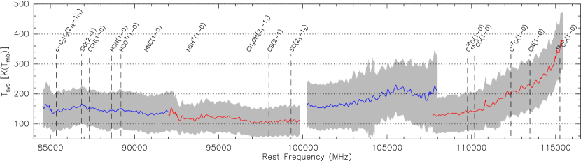
Figure 24: $T_{\mathrm{sys}}$ as a function of the frequency. The solid lines display the average $T_{\mathrm{sys}}$ and the grey shaded backgrounds show the $\pm 3\sigma$ interval at each frequency. The blue and red colors present the instantaneous 8$\mathrm{\,GHz}$-bandwidth of the lower and upper sidebands covered by the two tunings. The vertical dashed lines show the frequencies of the brightest lines studied here.

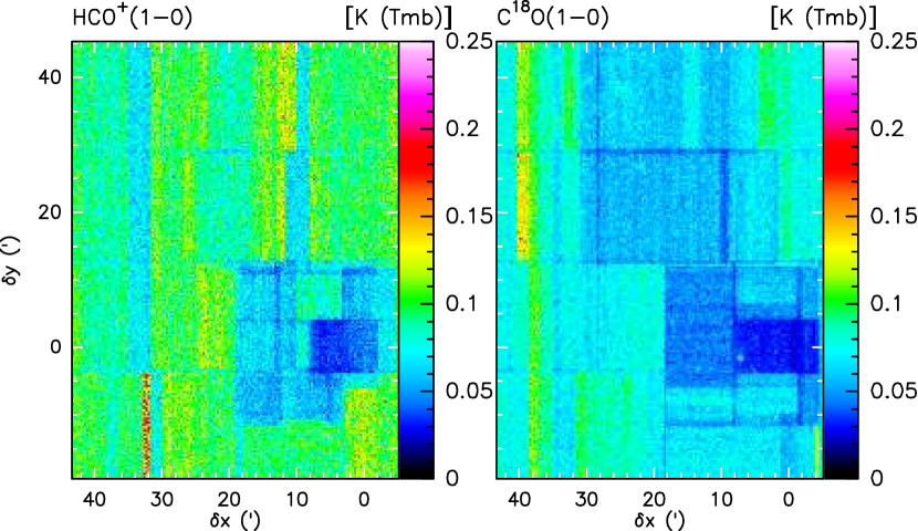
Figure 25: Typical spatial distribution of the RMS noise for two lines, each one belonging to one of the two tuning setups.

Table 12 summarizes the single-dish observations described in section 2.2. Figure 24 shows the average system temperature as a function of the rest frequency over the observed bandwidth. The mean (solid line) was computed over all the calibration measurements made during the observation and the shaded backgrounds display the $\pm 3\sigma$ interval that reflects both variations in the quality of the tuning and of the elevation of the source. The variations with the frequency come from a combination of hardware and atmosphere chromaticity effects. The optic and mixer performances vary with the observed radio-frequency and the cryogenic low noise amplifier performances vary with the instantaneous intermediate frequency. The atmospheric transparency mostly varies because of ozone lines present in the bandpass and because of the 118.75$\mathrm{\,GHz}$ (N=1-1, J=1-0) oxygen line whose wings strongly increase the $T_{\mathrm{sys}}$ at the upper end of the 3$\mathrm{\,mm}$ atmospheric window.

Figure 25 show the spatial distribution of the noise at an angular resolution of $31^{\prime\prime}$ for two lines, each one representing one of the two tunings. The region around the Horsehead and NGC 2023 were observed at the start of the project, before our observing strategy converged to the one described in Section 2.2. In particular, this area was covered at least once along the $\delta x$ axis, and once along the $\delta y$ axis. This explains why the noise properties of this region are different from other parts of the map. Except for this part of the map, the variations in the noise level reflect the variations of weather or elevation during the observations.

Appendix B Mean line profiles from different gas regimes

In Section 4, we derived the fraction of fluxes that come from different gas regimes in the lines averaged over the observed field of view. We here intend to deliver the tools to estimate the typical line fluxes when varying the number of lines of sight that sample the different gas regimes. We thus compute the mean line profiles over the same gas regimes as defined in Sections 4.1 and 4.2. Mixing these line profiles in different proportions would deliver a proxy for the line profile observed in GMCs that have different ratios of diffuse/dense gas or cold/warm gas.

Figures 26 and 28 show the mean line profiles for the different $A_{\mathrm{V}}^{\mathrm{}}$ and $T_{\mathrm{d}}^{\mathrm{}}$ regimes. Tables 13 and 14 present, for each transition, line integrated intensity averaged over the different $A_{\mathrm{V}}^{\mathrm{}}$ and $T_{\mathrm{d}}^{\mathrm{}}$ masked regions. Figure 27 and 29 show these line integrated intensities in percentage of the integrated intensity averaged over the full field of view. These later plots indicate the potential intensity gain that can be expected when resolving the regions that are compact.

As expected, the intensity increases with the visual extinction, i.e. with the column density of matter. However, the increase is only a factor 2 for the $\mathrm{{}^{12}CO}$ $\mathrm{(1-0)}$ line while it reaches a factor of almost 30 for the $\mathrm{N_{2}H^{+}}$ $\mathrm{(1-0)}$ line. All lines except $\mathrm{N_{2}H^{+}}$ $\mathrm{(1-0)}$ have a mean integrated intensity that increases by a factor 2 in the filamentary gas $(6\leq A_{\mathrm{V}}^{\mathrm{}}<15)$. The mean spectra at 10$\mathrm{\,pc}$ resolution are closer to the mean spectra over the translucent gas for all the lines, but for the $\mathrm{H^{13}CO^{+}}$, $\mathrm{CH_{3}OH}$, and $\mathrm{N_{2}H^{+}}$ low-J lines.

The $\mathrm{C_{2}H}$, $\mathrm{c-C_{3}H_{2}}$, $\mathrm{{}^{12}CN}$, $\mathrm{{}^{12}CO}$, $\mathrm{HCN}$, and $\mathrm{HCO^{+}}$ low-J lines have similar mean integrated intensities on regions of cold and hot dust, probably because some of the high visual extinction lines of sight are also associated with high dust temperature. The mean spectra of hot dust regions have significantly wider linewidths than the mean spectra of the cold dust regions, confirming that the gas temperature is significantly higher in at least the PDR parts along these lines of sight. The $\mathrm{HNC}$, $\mathrm{{}^{13}CO}$, $\mathrm{{}^{12}CS}$, $\mathrm{C^{17}O}$, $\mathrm{{}^{32}SO}$, $\mathrm{C^{18}O}$, $\mathrm{H^{13}CO^{+}}$, $\mathrm{CH_{3}OH}$, and $\mathrm{N_{2}H^{+}}$ low-J line mean integrated intensities are between 2 and 20 times brighter in the cold than in the hot dust regions. These lines are thus more characteristics of cold dense gas than the previous category. Finally, the mean line integrated intensity over the full field of view is closer to the line intensity integrated over the regions of warm and lukewarm dust regions than over the cold or hot dust regions.

Table 15: Line averaged intensities in $\mathrm{\,mK\,km\,s^{-1}}$ and in percentage of the total flux inside the four $A_{\mathrm{V}}^{\mathrm{}}$ mask regions.

Species	Transition	$0\leq A_{\mathrm{V}}^{\mathrm{}}<222$	$1\leq A_{\mathrm{V}}^{\mathrm{}}<2$	$2\leq A_{\mathrm{V}}^{\mathrm{}}<6$	$6\leq A_{\mathrm{V}}^{\mathrm{}}<15$	$15\leq A_{\mathrm{V}}^{\mathrm{}}<222$
$\mathrm{{}^{12}CO}$	$1-0$	$33000$ $(100\%)$	$3300$ $(9.9\%)$	$36000$ $(110\%)$	$65000$ $(200\%)$	$77000$ $(230\%)$
$\mathrm{{}^{13}CO}$	$1-0$	$6200$ $(100\%)$	$350$ $(5.7\%)$	$4900$ $(79\%)$	$15000$ $(230\%)$	$29000$ $(470\%)$
$\mathrm{HCO^{+}}$	$1-0$	$980$ $(100\%)$	$110$ $(11\%)$	$840$ $(85\%)$	$2000$ $(210\%)$	$4700$ $(480\%)$
$\mathrm{HCN}$	$1-0$	$590$ $(100\%)$	$40$ $(6.9\%)$	$440$ $(75\%)$	$1300$ $(230\%)$	$3200$ $(550\%)$
$\mathrm{C^{18}O}$	$1-0$	$430$ $(100\%)$	$8.4$ $(1.9\%)$	$210$ $(49\%)$	$1100$ $(240\%)$	$3800$ $(880\%)$
$\mathrm{{}^{12}CS}$	$2-1$	$370$ $(100\%)$	$9.9$ $(2.7\%)$	$190$ $(52\%)$	$800$ $(220\%)$	$3700$ $(990\%)$
$\mathrm{{}^{12}CN}$	$1-0$	$350$ $(100\%)$	$36$ $(10\%)$	$250$ $(70\%)$	$810$ $(230\%)$	$2100$ $(590\%)$
$\mathrm{HNC}$	$1-0$	$310$ $(100\%)$	$26$ $(8.4\%)$	$190$ $(61\%)$	$650$ $(210\%)$	$2600$ $(830\%)$
$\mathrm{C_{2}H}$	$1-0$	$270$ $(100\%)$	$47$ $(18\%)$	$230$ $(87\%)$	$510$ $(190\%)$	$1400$ $(520\%)$
$\mathrm{{}^{32}SO}$	$2-1$	$200$ $(100\%)$	$6.8$ $(3.4\%)$	$100$ $(50\%)$	$460$ $(230\%)$	$1900$ $(940\%)$
$\mathrm{C^{17}O}$	$1-0$	$100$ $(100\%)$	$23$ $(22\%)$	$53$ $(53\%)$	$230$ $(220\%)$	$800$ $(780\%)$
$\mathrm{c-C_{3}H_{2}}$	$2-1$	$87$ $(100\%)$	$15$ $(18\%)$	$73$ $(84\%)$	$170$ $(190\%)$	$450$ $(520\%)$
$\mathrm{H^{13}CO^{+}}$	$1-0$	$33$ $(100\%)$	$0.87$ $(2.6\%)$	$4.9$ $(15\%)$	$57$ $(170\%)$	$560$ $(1700\%)$
$\mathrm{N_{2}H^{+}}$	$1-0$	$29$ $(100\%)$	$-13$ $(-45\%)$	$5$ $(17\%)$	$25$ $(85\%)$	$780$ $(2700\%)$
$\mathrm{CH_{3}OH}$	$2-1$	$27$ $(100\%)$	$4.7$ $(17\%)$	$3.3$ $(12\%)$	$57$ $(210\%)$	$390$ $(1500\%)$

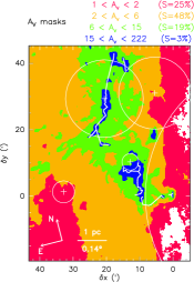
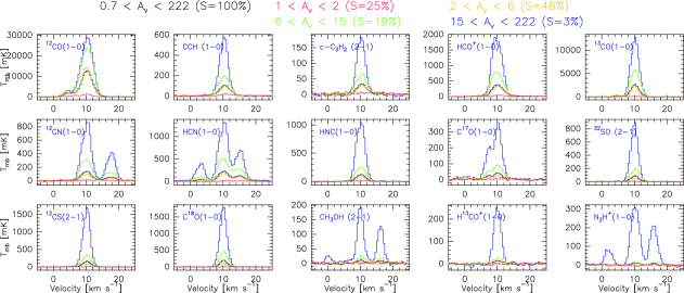
Figure 26: Same as Fig. 6, except that the spectra show the temperature intensity averaged over the different masks.

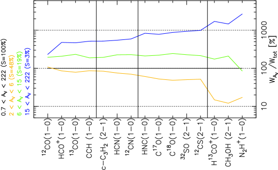
Figure 27: For each transition, line integrated intensity computed over the same velocity range divided by the line integrated intensity computed over the surface where $A_{\mathrm{V}}^{\mathrm{}}\geq 15$. All line integrated intensities are computed between 9 and 12$\mathrm{\,km\,s^{-1}}$. The black vertical lines define the groups of lines described in Section 4.1.

Table 16: Line intensities averaged over $[9,12\mathrm{\,km\,s^{-1}}]$ inside the four $T_{\mathrm{d}}^{\mathrm{}}$ mask regions in $\mathrm{\,mK\,km\,s^{-1}}$ and in percentage of the intensity of the cold dust region.

Species	Transition	$16\leq T_{\mathrm{d}}^{\mathrm{}}<100$	$16\leq T_{\mathrm{d}}^{\mathrm{}}<19.5$	$19.5\leq T_{\mathrm{d}}^{\mathrm{}}<23.5$	$23.5\leq T_{\mathrm{d}}^{\mathrm{}}<32$	$32\leq T_{\mathrm{d}}^{\mathrm{}}<100$
$\mathrm{{}^{12}CO}$	$1-0$	$33000$ $(100\%)$	$44000$ $(130\%)$	$28000$ $(85\%)$	$31000$ $(94\%)$	$56000$ $(170\%)$
$\mathrm{{}^{13}CO}$	$1-0$	$6200$ $(100\%)$	$15000$ $(250\%)$	$5800$ $(92\%)$	$5000$ $(81\%)$	$10000$ $(170\%)$
$\mathrm{HCO^{+}}$	$1-0$	$980$ $(100\%)$	$2500$ $(250\%)$	$670$ $(68\%)$	$870$ $(89\%)$	$2200$ $(220\%)$
$\mathrm{HCN}$	$1-0$	$590$ $(100\%)$	$1400$ $(230\%)$	$390$ $(66\%)$	$500$ $(85\%)$	$1500$ $(250\%)$
$\mathrm{C^{18}O}$	$1-0$	$430$ $(100\%)$	$2100$ $(490\%)$	$420$ $(99\%)$	$290$ $(67\%)$	$660$ $(150\%)$
$\mathrm{{}^{12}CS}$	$2-1$	$370$ $(100\%)$	$1700$ $(450\%)$	$290$ $(78\%)$	$250$ $(69\%)$	$830$ $(230\%)$
$\mathrm{{}^{12}CN}$	$1-0$	$350$ $(100\%)$	$770$ $(220\%)$	$220$ $(61\%)$	$290$ $(81\%)$	$970$ $(280\%)$
$\mathrm{HNC}$	$1-0$	$310$ $(100\%)$	$1300$ $(430\%)$	$210$ $(69\%)$	$240$ $(79\%)$	$690$ $(230\%)$
$\mathrm{C_{2}H}$	$1-0$	$270$ $(100\%)$	$460$ $(170\%)$	$150$ $(57\%)$	$260$ $(97\%)$	$670$ $(250\%)$
$\mathrm{{}^{32}SO}$	$2-1$	$200$ $(100\%)$	$1200$ $(610\%)$	$170$ $(84\%)$	$140$ $(70\%)$	$350$ $(180\%)$
$\mathrm{C^{17}O}$	$1-0$	$100$ $(100\%)$	$440$ $(430\%)$	$100$ $(99\%)$	$73$ $(72\%)$	$150$ $(140\%)$
$\mathrm{c-C_{3}H_{2}}$	$2-1$	$87$ $(100\%)$	$200$ $(230\%)$	$50$ $(57\%)$	$85$ $(97\%)$	$210$ $(240\%)$
$\mathrm{H^{13}CO^{+}}$	$1-0$	$33$ $(100\%)$	$290$ $(890\%)$	$25$ $(75\%)$	$19$ $(58\%)$	$67$ $(210\%)$
$\mathrm{N_{2}H^{+}}$	$1-0$	$29$ $(100\%)$	$420$ $(1500\%)$	$25$ $(86\%)$	$11$ $(37\%)$	$44$ $(150\%)$
$\mathrm{CH_{3}OH}$	$2-1$	$27$ $(100\%)$	$260$ $(970\%)$	$21$ $(78\%)$	$19$ $(72\%)$	$38$ $(140\%)$

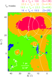
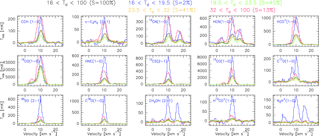
Figure 28: Same as Fig. 8, except that the spectra show the temperature intensity averaged over the different masks.

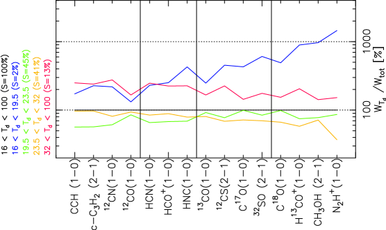
Figure 29: For each transition, line integrated intensity divided by the line integrated intensity computed over the surface where $T_{\mathrm{d}}^{\mathrm{}}<20\mathrm{\,K}$. All line integrated intensities are computed between 9 and 12$\mathrm{\,km\,s^{-1}}$. The black vertical lines define the groups of lines described in Section 4.2.