IFUP-TH-2016
Confinement, NonAbelian monopoles, and 2D ${\mathbb{C}}P^{N-1}$ model on the worldsheet of finite-length strings

Abstract

Quark confinement is proposed to be a dual Meissner effect of nonAbelian kind. Important hints come from physics of strongly-coupled infrared-fixed-point theories in ${\cal N}=2$ supersymmetric QCD, which turn into confining vacua under a small relevant perturbation. The quest for the semiclassical origin of the nonAbelian monopoles, ubiquitous as the infrared degrees of freedom in supersymmetric gauge theories, motivates us to study the quantum dynamics of 2D ${\mathbb{C}}P^{N-1}$ model defined on a finite-width worldstrip, with various boundary conditions. The model is found to possess a unique phase (”confinement phase”), independent of the length of the string, showing the quantum persistence of the nonAbelian monopole.

1 Confinement as non-Abelian dual Meissner effect

In general asymptotic-free gauge theories the renormalization-group (RG) flow looks like in Fig. 1. The system in a UV fixed point, which is a free Yang-Mills theory, flows into an infrared fixed point (FP). In some cases the system approaches in the infrared a FP conformally invariant theory (CFT), but before reaching it, the RG path deviates from the one to CFT to a nearby vacuum in a confinement phase, with mass generation and with the elementary charges (the quarks) confined by a vortex like chromoelectric strings. Such a deviation in the RG flow at the final stage is caused by some relevant operator, which could either be present in the original UV Lagrangian, or may be generated dynamically by the gauge dynamics itself.

Figure 1: RG flow of general aymptotically free gauge theories

One usually thinks that confinement and conformal invariance are two opposite notions: in one case one has dynamical mass generation and symmetry breaking, in the other, no condensation, no mass gap, no symmetry breaking. How can such two different phenomena be ”close to each other”?

The answer is that in asymptotically-free gauge theories, the degrees of freedom in the low-energy effective theory can be different from those in the underlying UV theory. Instead of the original quarks and gluons, the solitonic, magnetic monopoles and dual gauge fields may take up the role of the carrier of the low-energy dynamics. These degrees of freedom are shared between the infrared fixed-point theory and the nearby confining vacuum. There are many examples of this kind of RG flows, especially in the context of softly broken ${\cal N}=2$ supersymmetric gauge theories [1]-[12].

In theories described by such a RG flow, confinement is described by the same degrees of freedom characterizing the nearby CFT. Thus the particular types of confining vacua - the nature of the degrees of freedom and their interactions - are related to the possible types of the nearby CFT. Such a correspondence could be particularly welcome, when the nearby fixed point is a strongly-coupled conformal theory, where relatively nonlocal degrees of freedom such as (nonAbelian) monopoles, dyons and quarks all appear simultaneously as the infrared degrees of freedom. These theories are not described by a local Lagrangian and in general are quite hard to analyze [5],[6]. Strong constraints on CFT may however allow us to draw useful conclusions about the behavior of the system under the deformation into the nearby confinement vacuum, hence about the confinement mechanism itself.

2 QCD

Are these considerations relevant for the standard QCD? The well-known idea, by Nambu, Mandelstam and ’t Hooft [13], is that somehow the $SU(3)$ color gauge interactions undergo dynamical Abelianization $SU(3)\to U(1)\times U(1)$ , and that the low-energy degrees of freedom (the monopoles of the two $U(1)$ (dual) theories) somehow condense, and give rise to confinement in a scenario similar to the type II superconductivity. The quarks (the chromoelectric charges) would thus be confined by a dual Meissner mechanism.

The problem is that the presence of two confining strings $\Pi_{1}(U(1)\times U(1))={\mathbb{Z}}\times{\mathbb{Z}}\;$ implies the doubling of meson spectra, not observed in Nature. Another difficulty is the following. If the confinement and chiral symmetry breaking are related, the most natural explanation is that the Abelian monopoles carry the $SU_{L}(2)\times SU_{R}(2)$ chiral symmetry charges, $M_{i}^{j}\;,$ and their ”diagonal” condensation

$$\langle M_{i}^{j}\rangle=\delta_{i}^{l}\,\Lambda\;,$$ (2.1)

explains the two phenomena at the same time. However a $U(1)^{2}$ theory with $N_{f}\times N_{f}=4$ scalar monopoles would have an accidental $SU(4)$ symmetry, broken to $SU(2)$, implying $12$ Nambu-Goldstone bosons, again not observed in Nature. Finally, $U(1)$ theories are weakly coupled at low energies: why should monopoles condense?

A possible alternative is that the $SU(3)$ gauge symmetry dynamically reduces as $SU(3)\to SU(2)\times U(1)\;;$ the condensation of the nonAbelian monopoles would break the remaining gauge symmetries and produce a vacuum in which the quarks are confined in a dual Meissner effect, of a nonAbelian type. As $\Pi_{1}(SU(2)\times U(1))={\mathbb{Z}}\;,$ the problem of the meson spectrum doubling is naturally solved. A strongly interacting, nonAbelian magnetic monopoles may also be welcome as it could provide a natural dynamical mechanism for monopole condensation.

One is aware of the fact that a system of strongly interacting nonAbelian monopoles can be something rather difficult to analyze. Let us note however that, unlike the ”difficulties” mentioned earlier, this is a difficulty for us, not for Nature.

2.1 NonAbelian monopoles

The concept of nonAbelian monopoles turned out to be peculiarly evasive. A famous difficulty is the so-called topological obstruction [14] Another is an infinitesimal version of this: gauge zeromodes around a soliton monopole solution are non-normalizable [15]. This means that the standard quantization procedure to construct the ${\underline{N}}$ gauge multiplet of monopoles through the action of the zero-mode creation operators does not work.

Both these classical ”difficulties” however miss the fundamental aspect of the nonAbelian monopoles, expressed by the well-known GNO (Goddard-Nuyts-Olive) quantization condition [16]. The asymptotic behavior of the monopole solution generated by the gauge symmetry breaking, $G\to H$, can be written in an appropriate gauge as,

$$F_{ij}=\epsilon_{ijk}\frac{r^{k}}{r^{3}}(\beta\cdot{\bf H})\;,$$ (2.2)

where $\bf H$ is the Cartan subalgebra generators of the ”unbroken” gauge group $H$, and $\beta$ is some vector, characterizing each solution, having the number of components equal to the rank of the subgroup $H$. GNO found that the consistency requires that

$$2\beta\cdot\alpha\in{\mathbb{Z}}\;,$$ (2.3)

where $\alpha$ are the root vectors of $H$. Eq. (2.3) naturally generalizes the famous Dirac quantization condition. The GNO condition states that the magnetic monopoles in the broken gauge theory $G/H$ are labeled and classified by the weight vectors of the dual gauge group ${\tilde{H}}$, which is generated by the (nonzero) dual root vectors

$$\alpha^{*}=\frac{\alpha}{\alpha\cdot\alpha}\;,$$ (2.4)

and not by the original group $H$ itself. Examples of pairs of dual groups are given in Table 1.

Table 1: Examples of dual pairs of groups

$H$	${\tilde{H}}$
$U(N)$	$U(N)$
$SU(N)$	$SU(N)/Z_{N}$
$SO(N)$	$Spin(N)$
$SO(2N+1)$	$USp(2N)$

3 Hints from ${\cal N}=2$ supersymmetric QCD

In spite of the classical ”difficulties” mentioned above, monopoles with nonAbelian (dual) gauge charges are ubiquitous in ${\cal N}=2$ supersymmetric gauge theories: they appear as low-energy effective degrees of freedom, in certain singular vacua . They are pointlike particles of the low-energy effective theory, and act as carriers of the dual (magnetic) gauge charges, as well as of the flavor symmetries of the underlying theory. Under certain circumstances (e.g., appropriate ${\cal N}=1$ relevant perturbation) they condense and induce confinement and chiral symmetry breaking. Exactly how this occurs depends on the model considered, on the gauge and flavor groups, and on the particular infrared vacuum considered.

(i)

Abelian dual superconductivity.

This occurs in ${\cal N}=2$ $SU(2)$ gauge theories [1], with number of flavors, $N_{f}=1,2,3$. The system dynamically Abelianizes, and Abelian monopoles condense upon some ${\cal N}=1$ perturbation (the adjoint scalar mass term, which is a relevant operator). Similar phenomena occur in pure ${\cal N}=2$ $SU(N)$ theories in simple singularities of the vacuum moduli space [2]. This is a beautiful phenomenon, but appears to share little with the real-world QCD.

(ii)

NonAbelian monopole condensation.

In ${\cal N}=2$ supersymmetric SQCD, there are so-called $r$-vacua [3, 4], in which the low-energy dual gauge group is $SU(r)\times U(1)^{N-r}$. The effective degrees of freedom there turn out to be nonAbelian magnetic monopoles in the ${\underline{r}}$ representation of the dual $SU(r)$ gauge group, and in ${\underline{N_{f}}}$ of the flavor $SU(N_{f})$ symmetry group. The possible values of $r$ run up to $r\leq[N_{f}/2]$. The nonAbelian monopoles are weakly coupled, and the dual theory is infrared free. Again, these are interesting theories, but do not resemble the real-world strong interactions (weakly-coupled magnetic monopoles are not what we observe at low-energies).

(iii)

NonAbelian monopoles interacting strongly.

The most intriguing systems are the confining vacua arising from (or near) the strongly-coupled infrared (super) conformal points. In general these systems involve relatively nonlocal degrees of freedom (monopole, dyons and quarks, all becoming massless and interacting together), which defy a local Lagrangian description. Not surprisingly these are the least studied systems, but thanks to some key inputs by Argyres, Seiberg and others [7]-[11] there have been some significant development recently in understanding confinement near the so-called superconformal points of highest criticality (the Eguchi-Hori-Ito-Yang vacua) [6].

3.1 ${\cal N}=1$ perturbation of the AD vacua

Perhaps the most suggestive result among the vacua of the type (iii) above, is the one discussed in [12]. It was found that the ${\cal N}=2$ Argyres-Douglas vacua arising from coalescing $r$ vacua - which is a strongly coupled, nonlocal infrared fixed-point conformal theory of monopoles, dyons and quarks, when deformed by a simple adjoint mass perturbation, make a metamorphosis into an ${\cal N}=1$ superconformal fixed point, described by free mesons in the adjoint representation of the flavor $SU(N_{f})$ group! Upon further deformation (e.g., some shift of masses), the system goes into confinement phase, described by the same massless degrees of freedom, which now act as the Nambu-Goldstone bosons of the symmetry breaking.

4 NonAbelian monopoles from monopole-vortex
antimonopole soliton complex

There remains the problem of understanding the nonAbelian monopoles appearing in the various vacua of ${\cal N}=2$ supersymmetric gauge theories as the low-energy effective degrees of freedom, from the semiclassical point of view, i.e., by relating them to the more familiar picture of topologcal solitons made of the underlying gauge and matter fields. The key idea is to consider a hierarchical gauge symmetry breaking, such as

$$SU(N+1)_{\rm color}\otimes SU(N)_{\rm flavor}\stackrel{{\scriptstyle v_{1}}}{{\longrightarrow}}(SU(N)\times U(1))_{\rm color}\otimes SU(N)_{\rm flavor}\stackrel{{\scriptstyle v_{2}}}{{\longrightarrow}}SU(N)_{C+F}\ ,$$ (4.1)

with

$$v_{1}\gg v_{2}\ ,$$ (4.2)

as in [18]-[23]. The presence of a nontrivial flavor group, and the persistence of an exact global symmetry in a so-called color-flavor locked phase, is crucial. A simple homotopy-group consideration shows that the monopoles generated at the high-energy symmetry breaking, having mass of order of $v_{1}/g$, must be the endpoints of the vortex arising from the low-energy gauge symmetry breaking. See Fig. 2 taken from [24]. This must be so as the vortices present in the system at low-energies ($\mu<v_{1}$) due to $\pi_{1}(SU(N)\times U(1))={\mathbf{Z}}$ must really be absent in the full theory as $\pi_{1}(SU(N+1)={\bf 1}$. At the same time the monopoles in the high-energy theory (at $\mu\gg v_{2}$) due to $\pi_{2}(SU(N+1)/SU(N)\times U(1))$ are after all absent once the low-energy symmetry breaking is taken into account ($\pi_{2}(SU(N+1))={\bf 1}$). The homotopy exact sequence connects each monopole to each vortex solution.

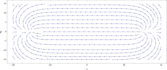
Figure 2: The magnetic field in the monopole-vortex-antimonopole soliton complex. Taken from Cipriani, et. al. [24]

The nonAbelian monopoles are to be understood in such a dynamical context, and not just as the properties of static, isolated classic field configurations on their own. This is perfectly consistent with the fact that the existence of nonAbelian monopoles, being a carrier of a nonAbelian gauge charges, depend critically on the phase of the system. For instance they would not appear in low energies if the system were to dynamically Abelianize at low energies.

There is actually an even stronger dynamical requirement in order for the concept of nonAbelian monopoles to survive quantum mechanically. This arises from the fact that the semiclassical monopoles and vortex, attached to each other by the homotopy connections, are subject to further quantum fluctuations of the internal, orientational zeromodes, which become important in the far infrared, $\mu\ll v_{2}$. These quantum effects are described by the $2D$ ${\mathbb{C}}P^{N-1}$ sigma model, in the case of the pure nonAbelian vortices [17]-[19], and by the $2D$-$1D$ coupled ${\mathbb{C}}P^{N-1}$ sigma model [20], in the case of the M-V-M soliton complex [21]-[24] of interest here.

The monopoles in this context appear in ${\underline{N}}$ of the $SU(N)$ isometry group of the ${\mathbb{C}}P^{N-1}$. This fact defines them as nonAbelian monopoles.

The fate of the nonAbelian monopoles as quantum mechanical entity is then linked to the phase of the low-energy ${\mathbb{C}}P^{N-1}$ effective action, defined on a finite-width worldsheet of the nonAbelian string with a monopole and an antimonopole attached at its ends.

5 ${\mathbb{C}}P^{N-1}$ model in a finite-width worldstrip

These considerations have led us recently to study [25] the ${\mathbb{C}}P^{N-1}$ sigma model defined on the finite-width world strip, $x\in[0,L]$:

$$S=\int dxdt\left((D_{\mu}n_{i})^{*}D^{\mu}n_{i}-\lambda(n_{i}^{*}n_{i}-r)\right)\;,$$ (5.1)

where $n^{i}$ with $i=1,\dots,N$ are $N$ complex scalar fields and the covariant derivative is $D_{\mu}=\partial_{\mu}-iA_{\mu}$. Configurations related by a $U(1)$ gauge transformation $z_{i}\to e^{i\alpha}z_{i}$ are equivalent: the $U(1)$ gauge field $A_{\mu}$ does not have a kinetic term in the classical action. $\lambda$ is a Lagrange multiplier that enforces the classical condition

$$n_{i}^{*}n_{i}=r\;,$$ (5.2)

where $r$ is the “size” of the ${\mathbb{C}}P^{N-1}$ manifold, related to the coupling constant $g$ by

$$r=\frac{4\pi}{g^{2}}\;.$$ (5.3)

The quantum properties of this model defined in infinite $2D$ spacetime, with $x\in[-\infty,\infty]$, and in the large $N$ approximation are well known [26, 27]. Since $n$ appears only quadratically in the Lagrangian, it can be integrated out to give

$$Z=\int[dA_{\mu}][d\lambda][dn_{i}][dn_{i}^{*}]\,e^{iS}=\int[dA_{\mu}][d\lambda]\,e^{i{S}_{{\rm eff}}}\ ,$$ (5.4)

leaving an effective action for $A_{\mu}$ and $\lambda$:

$${S}_{{\rm eff}}=\int d^{2}x\left(N\,{\rm tr}\,{\rm log}(-D_{\mu}^{*}D^{\mu}+\lambda)-\lambda r\right)\;.$$ (5.5)

The condition of stationarity with respect to $\lambda(x)$ leads to the gap equation (in the Euclidean spacetime) as

$$r-N\,{\rm tr}\left(\frac{1}{-\partial_{\tau}^{2}-\partial_{x}^{2}+m^{2}}\right)=0\;,$$ (5.6)

where we have set $A_{\mu}=0$ and $\lambda=m^{2}$. An expectation value of $\lambda$ provides a mass for the $n_{i}$ particles. On the infinite line the spectrum is continuous and the gap equation reads

$$r=N\int_{0}^{\Lambda_{\rm UV}}\frac{kdk}{2\pi}\frac{1}{k^{2}+m^{2}}=\frac{N}{4\pi}\log{\left(\frac{\Lambda_{\rm UV}^{2}+m^{2}}{m^{2}}\right)}\;,$$ (5.7)

leading to the well-known scale-dependent renormalized coupling

$$r(\mu)=\frac{4\pi}{g(\mu)^{2}}\simeq\frac{N}{2\pi}\log{\left(\frac{\mu}{\Lambda}\right)}$$ (5.8)

and to a renormalization-group invariant scale, $\Lambda$, in terms of which the dynamically generated mass is given by

$$\langle\lambda\rangle=m^{2}=\Lambda^{2}\;.$$ (5.9)

Furthermore the kinetic term of the $A_{\mu}$ fields are generated by the one-loop graph, and leads to massless Coulomb field which confines the massive $n$ fields. Thus the spectrum is given by massive $n-n*$ mesons.

In order to define the model defined on the finite space interval, $x\in[0,L]$, one must specify the boundary condition for the $n$ fields. Motivated by the study of M-V-M complex [20], we consider the general boundary conditions including the case of Dirichlet-Dirichlet,

$$\hbox{D-D}:\qquad n_{1}(0)=n_{1}(L)=\sqrt{r}\;,\qquad n_{i}(0)=n_{i}(L)=0\;,\quad i>1\;.$$ (5.10)

and that of Neumann-Neumann

$$\hbox{N-N}:\qquad\partial_{x}n_{i}(0)=\partial_{x}n_{i}(L)=0\;.$$ (5.11)

The case of the periodic boundary condition, which has been extensively studied in the literature, is also considered.

The main question one asks here is whether or not the isometry group of the ${\mathbb{C}}P^{N-1}$, $SU(N)$, is spontaneously broken (Higgs phase) or not (confinement phase).

The $N$ fields can be separated into a classical component $\sigma\equiv n_{1}$ and the rest, $n^{i}$ ($i=2,\dots,N$). Integrating over the $N-1$ remaining fields yields the following effective action

$${S}_{{\rm eff}}=\int d^{2}x\left((N-1)\,{\rm tr}\,{\rm log}(-D_{\mu}D^{\mu}+\lambda)+(D_{\mu}\sigma)^{*}D^{\mu}\sigma-\lambda(|\sigma|^{2}-r)\right)\;.$$ (5.12)

One can take $\sigma$ real and set the gauge field to zero, and consider the leading contribution at large $N$ only. The total energy can formally be written as

$$E=N\sum_{n}\omega_{n}+\int_{0}^{L}\left((\partial_{x}\sigma)^{2}+\lambda(\sigma^{2}-r)\right)dx\;,$$ (5.13)

where $\omega_{n}^{2}$ are the eigenvalues of the operator

$$\left(-\partial_{x}^{2}+\lambda(x)\right)f_{n}(x)=\omega_{n}^{2}\ f_{n}(x)\;,$$ (5.14)

and $f_{n}$ are the corresponding eigenfunctions. As we are working in the large $N$ approximations we do not distinguish $N-1$ from $N$. The eigenfunctions $f_{n}$ can be taken to be real and orthonormal in $[0,L]$:

$$\int_{0}^{L}dx\,f_{n}(x)f_{m}(x)=\delta_{n\,m}\;.$$ (5.15)

The functional variation of $E$ with respect to the fields $\sigma(x)$ and $\lambda(x)$ yields the coupled equations

$$\partial_{x}^{2}\sigma(x)-\lambda(x)\sigma(x)=0,\qquad\frac{N}{2}\,\sum_{n}\frac{f_{n}(x)^{2}}{\omega_{n}}+\sigma(x)^{2}-r=0\,,$$ (5.16)

which generalizes the gap equation (5.6).

The set of equations (5.14)-(5.16) must be solved for two functions $\lambda(x)$ and $\sigma(x)$. Apparently this presents a rather formidable problem: they represent complicated nonlinear coupled equations. We solved these functional saddle-point equations numerically by using an idea similar to that of Hartree’s approximation in atomic physics. Namely, starting with some trial $\lambda(x)$, we solve the wave equations (5.14) for many levels (up to some ultraviolet cutoff mode) and insert them into the second of (5.16). We find $\sigma(x)$ after subtracting the logarithmic divergence and renormalizing the coupling constant $r$; the resulting finite $\sigma(x)$ is used to obtain $\lambda(x)$ of the next iteration, from the first of (5.16). Th procedure can be repeated until a consistent set of $\lambda(x)$ and $\sigma(x)$ are found.

A subtle point is that the behavior of the functions $\lambda(x)$ and $\sigma(x)$ near the boundaries $x=0,L$ turns out to be singular,

$$\sigma^{2}\simeq\frac{N}{2\pi}\log{\frac{1}{x}}\;,\qquad\lambda(x)\simeq\frac{1}{2\,x^{2}\log{1/x}}\;,$$ (5.17)

and similarly for $x\to L-x$. This result can be traced back to the fact that at the boundaries where quantum effects are suppressed, $\sigma(x)=n_{1}(x)$ must account for the classical radius of the ${\mathbb{C}}P^{N-1}$, $\sqrt{r}$, which is large (see (5.10), (5.7)). The numerical solution described above indeed produces this behavior.

The results for values of $L\Lambda$ up to $4$ are shown in Figure 4, 4, for $\Lambda=1$ fixed. From the figures one sees the expected pattern emerging: by going to larger $L$ at fixed $\Lambda$ one expects to recover the confined phase of the standard ${\mathbb{C}}P^{N-1}$ sigma model, Eq. (5.9). We indeed see that $\sqrt{\lambda(x)}\to\Lambda$ in the middle of the interval whereas the condensate $\sigma$ approaches zero there at the same time. The effects of the boundary appear to remain concentrated near the two extremes and not to significantly propagate beyond $1/\Lambda$.

The results found on the ${\mathbb{C}}P^{N-1}$ sigma model defined on the finite-width world strip, $x\in[0,L]$, can be summarized as follows [25].

(i)

The solution of the generalized gap equations (the functional saddle point equations, (5.14)-(5.16), is found to be unique.

(ii)

In particular, no ”Higgs phase” solution with $\langle\lambda\rangle=0\;,\langle\sigma\rangle\sim\Lambda\;\,$ exists.

(iii)

In other words no phase transition from the ”confinement phase” with $\langle\lambda\rangle\sim\Lambda\;,\langle\sigma\rangle=0\;\,$ to the ”Higgs phase” occur. Our conclusion differs from that of Milekhin [28]. The discrepancy may be traced to the fact that due to the boundary condition, the translational invariance Ansatz used in [28] is not valid.

(iv)

At large $L$ the known result in the standard ${\mathbb{C}}P^{N-1}$ sigma model on infinite $2D$ spacetime, Eq. (5.9), is seen to emerge from our analysis.

(v)

It turns out that exactly the same results on $\lambda(x)$ and $\sigma(x)$ are found for both DD and NN conditions. Though such a result may not be obvious at all, it can be understood by observing that the classical large ${\mathbb{C}}P^{N-1}$ radius must be attained independently of the particular form of the boundary condition, as at the boundaries the quantum fluctuations are suppressed.

(vi)

This, and the fact that the phase transition to the Higgs phase is absent in our case, can be understood by the fact that the system interpolates between an effectively $1D$ quantum system (quantum mechanics) at $L\ll 1/\Lambda$ to genuine $2D$ quantum field theory at large $L$, $L\gg 1/\Lambda$.

(vii)

Dynamical symmetry breaking of the $SU(N)$ isometry group (the Higgs phase) does not occur. This leaves the nonAbelian nature of the monopoles at the endpoints of the worldstrip intact: it transforms as ${\underline{N}}$ of $SU(N)$.

(viii)

It was found recently that this system with periodic boundary condition allows two possible phases, the Higgs phase at small $L$ ($\leq 1/\Lambda$) and the confinement phase at larger $L$. We note that even at small $L$ the system maintains $2D$ quantum field theory characteristics in this case, in contrast to the DD or NN conditions discussed above.

6 Conclusion

To conclude, the concept of nonAbelian monopole is consistent with quantum mechanics. In a system in which gauge symmetry is broken hierarchically as in (4.1), monopoles appear as ${\underline{N}}$ of the isometry $SU(N)$ group of ${\mathbb{C}}P^{N-1}$, which describes the effective, low-energy dynamics of the $M-V-M$ soliton complex. The $SU(N)$ transformation corresponds to nonlocal field transformations in terms of the original field variables, as the ${\mathbb{C}}P^{N-1}$ model describes fluctuations of the collective coordinates. This is perfectly consistent with the electromagnetic duality, albeit in an nonAbelian context. The isometry $SU(N)$ may be regarded as a disguise of the dual $SU(N)$ gauge symmetry (in confinement phase)

Figure 3: The dynamically generated mass of the $n_{i}$ fields, $\sqrt{\lambda(x)}$.

Figure 4: The VEV of the $\sigma=n_{1}$ field.

References

- [1] N. Seiberg and E. Witten, Nucl.Phys. B426 (1994) 19; Erratum ibid. B430 (1994) 485, hep-th/9407087; N. Seiberg and E. Witten, Nucl. Phys. B431 (1994) 484, hep-th/9408099.
- [2] P. C. Argyres and A. F. Faraggi, Phys. Rev. Lett 74 (1995) 3931, hep-th/9411047; A. Klemm, W. Lerche, S. Theisen and S. Yankielowicz, Phys. Lett. B344 (1995) 169, hep-th/9411048; Int. J. Mod. Phys. A11 (1996) 1929-1974, hep-th/9505150; A. Hanany and Y. Oz, Nucl. Phys. B452 (1995) 283, hep-th/9505075;
- [3] P.C. Argyres, M.R. Plesser and N. Seiberg, Nucl. Phys. B 471, 159 (1996) [arXiv:hep-th/9603042]; K. Hori, H. Ooguri and Y. Oz, Adv. Theor. Math. Phys. 1, 1 (1998) [arXiv:hep-th/9706082].
- [4] G. Carlino, K. Konishi and H. Murayama, Nucl. Phys. B 590, 37 (2000) [hep-th/0005076]; G. Carlino, K. Konishi, S. P. Kumar and H. Murayama, Nucl. Phys. B 608, 51 (2001) [hep-th/0104064].
- [5] P. C. Argyres, M. R. Plesser, N. Seiberg and E. Witten, Nucl. Phys. B 461 (1996) 71 [arXiv:hep-th/9511154].
- [6] T. Eguchi, K. Hori, K. Ito and S.-K. Yang, Nucl. Phys. B471 (1996) 430 [arXiv:hep-th/9603002].
- [7] P. C. Argyres and N. Seiberg, JHEP 0712, 088 (2007) [arXiv:0711.0054 [hep-th]].
- [8] D. Gaiotto, N. Seiberg and Y. Tachikawa, JHEP 1101, 078 (2011) [arXiv:1011.4568 [hep-th]].
- [9] L. Di Pietro and S. Giacomelli, JHEP 1202, 087 (2012) [arXiv:1108.6049 [hep-th]].
- [10] S. Giacomelli and K. Konishi, JHEP 1303, 009 (2013) [arXiv:1301.0420 [hep-th]];
- [11] S. Giacomelli, JHEP 1209, 040 (2012) [arXiv:1207.4037 [hep-th]].
- [12] S. Bolognesi, S. Giacomelli and K. Konishi, JHEP 1508, 131 (2015) [arXiv:1505.05801 [hep-th]].
- [13] G. ’t Hooft, Nucl. Phys. B 190, 455 (1981).: Nucl. Phys. B 153, 141 (1979).:
- [14] A. Abouelsaood, Nucl. Phys. B 226, 309 (1983); P. Nelson, A. Manohar, Phys. Rev. Lett. 50, 943 (1983); A. Balachandran, G. Marmo, M. Mukunda, J. Nilsson, E. Sudarshan, F. Zaccaria, Phys. Rev. Lett. 50, 1553 (1983); P. Nelson, S. Coleman, Nucl. Phys. B 227, 1 (1984).
- [15] N. Dorey, C. Fraser, T.J. Hollowood, M.A.C. Kneipp, Phys.Lett. B 383, 422 (1996) [arXiv: hep-th/9512116].
- [16] P. Goddard, J. Nuyts, D. Olive, Nucl. Phys. B 125, 1 (1977)
- [17] A. Hanany and D. Tong, JHEP 0307 (2003) 037 [arXiv:hep-th/0306150].
- [18] R. Auzzi, S. Bolognesi, J. Evslin, K. Konishi and A. Yung, Nucl. Phys. B 673 (2003) 187 [arXiv:hep-th/0307287].
- [19] A. Gorsky, M. Shifman, A. Yung, Phys. Rev. D71, 045010 (2005) [arXiv: hep-th/0412082].
- [20] C. Chatterjee and K. Konishi, JHEP 1409, 039 (2014) [arXiv:1406.5639 [hep-th]].
- [21] R. Auzzi, S. Bolognesi, J. Evslin and K. Konishi, Nucl. Phys. B 686 (2004) 119 [arXiv:hep-th/0312233]; M.A.C. Kneipp, Phys. Rev. D 69: 045007 (2004) [arXiv:hep-th/0308086].
- [22] M. Eto, L. Ferretti, K. Konishi, G. Marmorini, M. Nitta, K. Ohashi, W. Vinci and N. Yokoi, Nucl. Phys. B 780 161-187, 2007 [arXiv:hep-th/0611313].
- [23] K. Konishi, in Lecture Notes in Physics, 737 471 (2008), Springer [arXiv:hep-th/0702102].
- [24] M. Cipriani, D. Dorigoni, S. B. Gudnason, K. Konishi and A. Michelini, Phys. Rev. D 84, 045024 (2011) [arXiv:1106.4214 [hep-th]];
- [25] S. Bolognesi, K. Konishi and K. Ohashi, JHEP 1610, 073 (2016) [arXiv:1604.05630 [hep-th]].
- [26] A. D’Adda, M. Luscher and P. Di Vecchia, Nucl. Phys. B 146 (1978) 63.
- [27] E. Witten, Nucl. Phys. B 149 (1979) 285.
- [28] A. Milekhin, Phys. Rev. D 86, 105002 (2012) [arXiv:1207.0417 [hep-th]].
- [29] S. Monin, M. Shifman and A. Yung, Phys. Lev. D 92 (2015) 2, 025011 [arXiv:1505.07797 [hep-th]].