Check of a new non-perturbative mechanism for elementary fermion mass generation

Abstract:

We consider a field theoretical model where a SU(2) fermion doublet, subjected to non-Abelian gauge interactions, is also coupled to a complex scalar field doublet via a Yukawa and an irrelevant Wilson-like term. Despite the presence of these two chiral breaking operators in the Lagrangian, an exact symmetry acting on fermions and scalars prevents perturbative mass corrections. In the phase where fermions are massless (Wigner phase) the Yukawa coupling can be tuned to a critical value at which chiral transformations acting on fermions only become a symmetry of the theory (up to cutoff effects). In the Nambu-Goldstone phase of the critical theory a fermion mass term of dynamical origin is expected to arise in the Ward identities of the purely fermionic chiral transformations. Such a non-perturbative mechanism of dynamical mass generation can provide a “natural” (à la ’t Hooft) alternative to the Higgs mechanism adopted in the Standard Model. Here we lay down the theoretical framework necessary to demonstrate the existence of this mechanism by means of lattice simulations.

1 The mechanism in a simple model

In [1] a new non-perturbative (NP) mechanism for the elementary particle mass generation was conjectured. Existence and viability of this phenomenon can be tested in the toy model described by the Lagrangian

$${\cal L}_{\rm{toy}}(Q,A,\Phi)={\cal L}_{kin}(Q,A,\Phi)+{\cal V}(\Phi)+{\cal L}_{Wil}(Q,A,\Phi)+{\cal L}_{Yuk}(Q,\Phi)\,,$$ (1)

$$\quad{\cal L}_{kin}(Q,A,\Phi)=\frac{1}{4}(F\cdot F)+\bar{Q}_{L}{\mbox{$\not\!\!\cal D$}}Q_{L}+\bar{Q}_{R}{\mbox{$\not\!\!\cal D$}}\,Q_{R}+\frac{1}{2}{\,\hbox{tr}\,}\big{[}\partial_{\mu}\Phi^{\dagger}\partial_{\mu}\Phi\big{]}$$ (2)

$$\quad{\cal V}(\Phi)=\frac{\mu_{0}^{2}}{2}{\,\hbox{tr}\,}\big{[}\Phi^{\dagger}\Phi\big{]}+\frac{\lambda_{0}}{4}\big{(}{\,\hbox{tr}\,}\big{[}\Phi^{\dagger}\Phi\big{]}\big{)}^{2}$$ (3)

$$\quad{\cal L}_{Wil}(Q,A,\Phi)=\frac{b^{2}}{2}\rho\,\big{(}\bar{Q}_{L}{\overleftarrow{\cal D}}_{\mu}\Phi{\cal D}_{\mu}Q_{R}+\bar{Q}_{R}\overleftarrow{\cal D}_{\mu}\Phi^{\dagger}{\cal D}_{\mu}Q_{L}\big{)}$$ (4)

$$\quad{\cal L}_{Yuk}(Q,\Phi)=\ \eta\,\big{(}\bar{Q}_{L}\Phi Q_{R}+\bar{Q}_{R}\Phi^{\dagger}Q_{L}\big{)}\,,$$ (5)

where $b^{-1}=\Lambda_{UV}$ is the UV-cutoff. The Lagrangian (1) describes a non-Abelian gauge model where an SU(2) doublet of strongly interacting fermions is coupled to a complex scalar field via Wilson-like (eq. (4)) and Yukawa (eq. (5)) terms. For short we have used a compact SU(2)-like notation where $Q_{L}=(u_{L}\,\,d_{L})^{T}$ and $Q_{R}=(u_{R}\,\,d_{R})^{T}$ are fermion iso-doublets and $\Phi$ is a $2\times 2$ matrix with $\Phi=(\phi,-i\tau^{2}\phi^{*})$ and $\phi$ an iso-doublet of complex scalar fields.
The term ${\cal V}(\Phi)$ in eq. (3) is the standard quartic scalar potential where the (bare) parameters $\lambda_{0}$ and $\mu_{0}^{2}$ control the self-interaction and the mass of the scalar field. In the equations above we have introduced the covariant derivatives

$${\cal D}_{\mu}=\partial_{\mu}-ig_{s}\lambda^{a}A_{\mu}^{a}\,,\qquad\overleftarrow{\cal D}_{\mu}=\overleftarrow{\partial}_{\mu}+ig_{s}\lambda^{a}A_{\mu}^{a}\,,$$ (6)

where $A_{\mu}^{a}$ is the gluon field ($a=1,2,\dots,N_{c}^{2}-1$) with field strength $F_{\mu\nu}^{a}$. A crucial rôle in the model is played by the $d=4$ Yukawa term ${\cal L}_{Yuk}$ and the Wilson-like $d=6$ operator ${\cal L}_{Wil}$. For dimensional reasons the latter enters the Lagrangian multiplied by $b^{2}$.

Besides Lorentz, gauge and $C$, $P$, $T$, $CPF_{2}$ symmetries (see Appendix B of [1]), ${\cal L}_{\rm toy}$ is invariant under the following (global) transformations $\chi_{L}$ and $\chi_{R}$

$$\bullet\,\chi_{L}:\quad\tilde{\chi}_{L}\otimes(\Phi\to\Omega_{L}\Phi)\quad\quad\bullet\,\chi_{R}:\quad\tilde{\chi}_{R}\otimes(\Phi\to\Phi\Omega_{R}^{\dagger})$$ (7)

$$\tilde{\chi}_{L/R}:\left\{\begin{array}[]{l}Q_{L/R}\rightarrow\Omega_{L/R}Q_{L/R}\\ \hskip 113.81102pt\Omega_{L/R}\in{\mbox{SU}}(2)_{L/R}\\ \bar{Q}_{L/R}\rightarrow\bar{Q}_{L/R}\Omega_{L/R}^{\dagger}\\ \end{array}\right.$$ (11)

The model (1) is power-counting renormalizable (as LQCD is) with counter-terms constrained by the exact symmetries of the Lagrangian. In particular, owing to the presence of the scalar field and the related exact $\chi_{L}\otimes\chi_{R}$ symmetry, no power divergent fermion mass terms can be generated.

1.1 Fermionic chiral symmetry enhancement

For generic values of the parameters $(\rho,\eta)\neq(0,0)$ , ${\cal L}_{\rm{toy}}$ is not invariant under the chiral transformations $\tilde{\chi}_{L}$ and $\tilde{\chi}_{R}$ (eq. (11)). We are interested in the case where fermionic chiral symmetries are not exact as the breaking terms can polarize the vacuum under dynamical symmetry breaking due to strong interactions. To study possible enhancement of $\tilde{\chi}_{L}$ symmetry (by parity the same will hold also for $\tilde{\chi}_{R}$) we consider the (bare) $\tilde{\chi}_{L}$ WTIs, v.i.z.

$$\partial_{\mu}\langle\tilde{J}^{L\,i}_{\mu}(x)\,\hat{\cal O}(0)\rangle=\langle\tilde{\Delta}_{L}^{i}\hat{\cal O}(0)\rangle\delta(x)-\eta\,\langle\big{(}\bar{Q}_{L}\frac{\tau^{i}}{2}\Phi Q_{R}-\bar{Q}_{R}\Phi^{\dagger}\frac{\tau^{i}}{2}Q_{L}\big{)}(x)\,\hat{\cal O}(0)\rangle\!+$$

$$\phantom{\partial_{\mu}J^{L\,i}_{\mu}}-\frac{b^{2}}{2}\rho\,\langle\Big{(}\bar{Q}_{L}\overleftarrow{\cal D}_{\mu}\frac{\tau^{i}}{2}\Phi{\cal D}_{\mu}Q_{R}-\bar{Q}_{R}\overleftarrow{\cal D}_{\mu}\Phi^{\dagger}\frac{\tau^{i}}{2}{\cal D}_{\mu}Q_{L}\Big{)}(x)\,\hat{\cal O}(0)\rangle\,,$$ (12)

where $\tilde{\Delta}_{L}^{i}\hat{\cal O}(0)$ is the variations of $\hat{\cal O}(0)$ under $\tilde{\chi}_{L}$ and the non-conserved currents associated are

$$\tilde{J}_{\mu}^{L\,i}=\bar{Q}_{L}\gamma_{\mu}\frac{\tau^{i}}{2}Q_{L}-\frac{b^{2}}{2}\rho\Big{(}\bar{Q}_{L}\frac{\tau^{i}}{2}\Phi{\cal D}_{\mu}Q_{R}-\bar{Q}_{R}\overleftarrow{\cal D}_{\mu}\Phi^{\dagger}\frac{\tau^{i}}{2}Q_{L}\Big{)}\,.$$ (13)

Under renormalization the $d=6$ operator $\;O_{6}^{L\,i}=\frac{1}{2}\rho\Big{[}\bar{Q}_{L}\overleftarrow{\cal D}_{\mu}\frac{\tau^{i}}{2}\Phi{\cal D}_{\mu}Q_{R}-{\mbox{h.c.}}\Big{]}\;$ mixes with two $d=4$ operators, plus a set of six-dimensional ones that we globally denote by $[O_{6}^{L\,i}]_{sub}$ , v.i.z.

$$O_{6}^{L\,i}=\Big{[}O_{6}^{L\,i}\Big{]}_{sub}+\frac{Z_{\tilde{J}}-1}{b^{2}}\partial_{\mu}\tilde{J}^{L\,i}_{\mu}-\frac{\bar{\eta}}{b^{2}}\Big{[}\bar{Q}_{L}\frac{\tau^{i}}{2}\Phi Q_{R}-{\mbox{h.c.}}\Big{]}+\ldots$$ (14)

where $Z_{\tilde{J}}$ and $\bar{\eta}$ are functions of the dimensionless bare parameters entering (1) and hence depend on the subtracted scalar squared mass $\mu_{sub}^{2}=\mu_{0}^{2}-b^{2}\tau$ through the combination $b^{2}\mu_{sub}^{2}$ that is a negligible $O(b^{2})$ quantity [1]. Thus we write $Z_{\tilde{J}}=Z_{\tilde{J}}(\eta;g^{2}_{s},\rho,\lambda_{0})$ and $\bar{\eta}=\bar{\eta}(\eta;g^{2}_{s},\rho,\lambda_{0})$. Ellipses in the r.h.s. of eqs. (14) denote possible NP contributions to operator mixing, the possible occurrence of which will be discussed below. Plugging (14) in to (13) we get

$$\partial_{\mu}\langle Z_{\tilde{J}}\tilde{J}^{L,i}_{\mu}(x)\,\hat{\cal O}(0)\rangle\!=\!\langle\tilde{\Delta}_{L}^{i}\hat{\cal O}(0)\rangle\delta(x)-({\eta-\overline{\eta}})\,\langle{O_{Yuk}^{L,i}}(x)\,\hat{\cal O}(0)\rangle+{\ldots}+{\mbox{O}(b^{2})}.$$

Setting $\eta=\eta_{cr}(g^{2}_{s},\rho,\lambda_{0})$ such that $\eta_{cr}(g^{2}_{s},\rho,\lambda_{0})-\bar{\eta}(\eta_{cr};g^{2}_{s},\rho,\lambda_{0})=0$ the WTI become

$$\partial_{\mu}\langle Z_{\tilde{J}}\tilde{J}^{L,i}_{\mu}(x)\,\hat{\cal O}(0)\rangle\!=\!\langle\tilde{\Delta}_{L}^{i}\hat{\cal O}(0)\rangle\delta(x)+{\ldots}+{\mbox{O}(b^{2})}\,,$$ (15)

implying restoration of the fermionic $\tilde{\chi}_{L}\otimes\tilde{\chi}_{R}$ symmetries up to O($b^{2}$) UV cutoff effects.

1.2 Mass generation mechanism in the critical model

The physics of the model (1) at the critical value $\eta_{cr}$ crucially depends on whether the parameter $\mu^{2}_{0}$ is such that ${\cal V}(\Phi)$ has a unique minimum (Wigner phase of the $\chi_{L}$ symmetry, $\mu_{sub}^{2}>0$) or whether ${\cal V}(\Phi)$ develops the typical “mexican hat” shape (Nambu–Goldstone phase $\mu_{sub}^{2}<0$). In the Wigner phase no NP terms (i.e. ellipses) are expected to occur in the mixing pattern of eq. (14) and the transformations $\tilde{\chi}_{L}$ leads to eq. (15) without the ellipses.

In the Nambu-Goldstone phase a non-perturbative term is expected/conjectured[1] to appear in the mixing pattern of eqs. (14) leading to a WTI of the form

$$\partial_{\mu}\langle Z_{\tilde{J}}\tilde{J}^{L,i}_{\mu}(x)\,\hat{\cal O}(0)\rangle_{\eta_{cr}}=\langle\tilde{\Delta}_{L}^{i}\hat{\cal O}(0)\rangle_{\eta_{cr}}\delta(x)+\langle{C_{1}\Lambda_{s}[\overline{Q}_{L}\frac{\tau^{i}}{2}{\cal U}Q_{R}+\mbox{h.c.}]}\hat{\cal O}(0)\rangle+{\mbox{O}}(b^{2})$$

where

$${\cal U}=\frac{\Phi}{\sqrt{\Phi^{\dagger}\Phi}}=\frac{v+\sigma+i\overrightarrow{\tau}\overrightarrow{\pi}}{\sqrt{(v+\sigma)^{2}+\overrightarrow{\pi}\overrightarrow{\pi}}}\,.$$ (16)

${\cal U}$ is a dimensionless non-analytic function of $\Phi$ that has the same transformation properties as the latter under $\chi_{L}\times\chi_{R}$ and is well defined only if $\langle\Phi\rangle=v\neq 0$. In the local effective action $\Gamma^{NG}_{loc}$ of the theory the term $C_{1}\Lambda_{s}[\overline{Q}_{L}{\cal U}Q_{R}+\mbox{hc}]$ plays the role of a mass term. It does not stem from the Yukawa term and, interestingly, can give a natural (in the sense of ’t Hooft [2]) understanding of the fermion mass hierarchy problem (see discussion in [1]).

An idea of how the mechanism works can be obtained from a perturbative expansion where Feynman diagrams are evaluated with the Lagrangian (1) augmented by few extra term representing the expected $O(b^{2})$ NP effective vertices [1], as those shown in fig. 1 These vertices can be inserted together with $O(b^{2})$ vertices coming from the term (4) in diagrams like the ones depicted in fig. 2, giving rise to finite self-energy contributions.
It is worth noticing that if the mechanism we have conjectured really exist it will generate a NP mass therm for the fermions even in the quenched approximation where the vertices (b) and (c) of fig. 1, and thus the two rightmost diagrams of fig. 2, are still present.

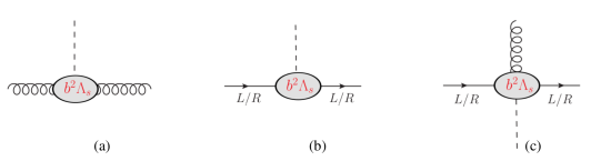
Figure 1: Some of the NP O($b^{2}\Lambda_{s}\alpha_{s}^{2}$) effective vertices that are conjectured to arise [1] in the Nambu-Goldstone phase of the model.

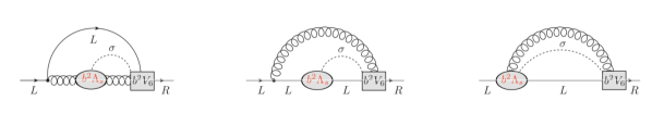
Figure 2: Typical lowest order self-energy ”diagrams” giving rise to dynamically generated quark mass terms. The grey box represents the insertion of the Wilson-like vertex stemming from ${\cal L}_{Will}$. The dotted line represents the propagation of a scalar particle. The $b^{-4}$ loop divergency is cancelled by the two vertices O$(b^{2})$ giving rise to a finite result.

2 Lattice quenched study of ${\cal L}_{toy}$: regularization and renormalization

Numerical simulations of lattice models with gauge, fermions and scalars are not common and technically challenging. In this first numerical study of the model (1) we can limit ourselves to a quenched-fermion simulation of the lattice regularized action

$${{S}_{{lat}}=b^{4}\sum_{x}\Big{\{}{\cal L}_{kin}^{YM}[U]+{\cal L}_{kin}^{sca}(\Phi)+{\cal V}(\Phi)}{+\overline{\Psi}{D_{lat}[U,\Phi]}\Psi\Big{\}}}$$ (17)

$${\cal L}_{kin}^{YM}[U]\,\,{\mbox{: SU($3$) plaquette action}}$$ (18)

$${\cal L}_{kin}^{sca}(\Phi)+{\cal V}(\Phi)=\frac{1}{2}{\,\hbox{tr}\,}[\Phi^{\dagger}(-\partial_{\mu}^{*}\partial_{\mu})\Phi]+\frac{\mu_{0}^{2}}{2}{\,\hbox{tr}\,}\big{[}\Phi^{\dagger}\Phi\big{]}+\frac{\lambda_{0}}{4}\big{(}{\,\hbox{tr}\,}\big{[}\Phi^{\dagger}\Phi\big{]}\big{)}^{2}\,,$$ (19)

where we have set $\Phi=\varphi_{0}1\!\!1+i\varphi_{j}\tau^{j}$

$$(D_{lat}[U,\Phi] \!\!\Psi)(x)=\gamma_{\mu}\widetilde{\nabla}_{\mu}\Psi(x)+\eta F(x)\Psi(x)-b^{2}\rho\frac{1}{2}F(x)\widetilde{\nabla}_{\mu}\widetilde{\nabla}_{\mu}\Psi(x)$$ (21)

$$-b^{2}\rho\frac{1}{4}\Big{[}(\partial_{\mu}F)(x)U_{\mu}(x)\widetilde{\nabla}_{\mu}\Psi(x+\hat{\mu})+(\partial_{\mu}^{*}F)(x)U_{\mu}^{\dagger}(x-\hat{\mu})\widetilde{\nabla}_{\mu}\Psi(x-\hat{\mu})\Big{]}\,,$$

with $\;F(x)\equiv[\varphi_{0}1\!\!1+i\gamma_{5}\tau^{j}\varphi_{j}](x)$ and the lattice derivatives defined as

$$\nabla_{\mu}f(x)\equiv\frac{1}{b}(U_{\mu}(x)f(x+\hat{\mu})-f(x))\quad\quad\nabla_{\mu}^{*}f(x)\equiv\frac{1}{b}(f(x)-U_{\mu}^{\dagger}(x-\hat{\mu})^{f}(x-\hat{\mu}))$$ (22)

$$\widetilde{\nabla}_{\mu}f(x)\equiv\frac{1}{2}(\nabla_{\mu}+\nabla_{\mu}^{*})F(x)$$ (23)

The Lagrangian (17) describes $2$ flavours $\Psi^{T}=(u,d)\times 16$ doublers even in the $b\rightarrow 0$ limit. In fact, the Wilson-like term does not remove the doublers because it has dimension six. This makes no harm in this quenched study aimed at testing whether the mass generation mechanism occurs at all. For further unquenched studies domain-wall [3] or overlap fermion [4] will be required.

One can check that the action (17) is invariant under global $\chi_{L}\otimes\chi_{R}$ transformations (see eq.(7)) and the lattice version of the discrete $P$, $T$, $C$ and $CPF_{2}$ symmetries. The discretization of the covariant derivatives in the Wilson-like terms of $D_{lat}$ (the ones with coefficient $\rho$) is chosen so that the lattice action $S_{lat}$ is exactly invariant under the ”spectrum doubling symmetry” [5].

$$\Psi(x)\to\Psi^{\prime}(x)=e^{-ix\cdot\pi_{H}}M_{H}\Psi(x)\quad\quad\overline{\Psi}(x)\to\overline{\Psi}^{\prime}(x)=\overline{\Psi}(x)M_{H}^{\dagger}e^{ix\cdot\pi_{H}}$$ (24)

where $H$ is an ordered set of four-vector indices $H\equiv\{\mu_{1},...,\mu_{h}\},\,(\mu_{1}<\mu_{2}<...<\mu_{h})$. For $0\leq h\leq 4$ there are 16 four-vector $\pi_{H}$ with $\pi_{H,\mu}=\pi$ if $\mu\in H$ otherwise $\pi_{H,\mu}=0$ and 16 matrices $M_{H}\equiv(i\gamma_{5}\gamma_{\mu_{1}})...(i\gamma_{5}\gamma_{\mu_{h}})$. The fact that only symmetric derivatives $\widetilde{\nabla}$ appear in the Wilson-like actions terms and the consequent ”spectrum doubling symmetry” guarantee that
a) at tree level the Wilson-like terms contribute only O($b^{2}$) effects as it is clear by noting e.g.

$$-b^{2}\sum_{x}e^{ipx}\widetilde{\nabla}_{\mu}\widetilde{\nabla}_{\mu}\Psi(x)|_{p=(0,b^{-1}\pi+\epsilon,0,0)\equiv\bar{p}}=\sin^{2}(\pi+b\epsilon)\tilde{\Psi}(p)|_{p=\bar{p}}=(b^{2}\epsilon^{2}+O(b^{4}\epsilon^{4}))\tilde{\Psi}(\bar{p})\,,$$ (25)

$$\sum_{y}e^{ipy}\gamma_{\mu}\widetilde{\nabla}_{\mu}\Psi(y)|_{p=(0,b^{-1}\pi+\epsilon,0,0)\equiv\bar{p}}=-ib^{-1}\gamma_{\mu}\sin(bp_{\mu})\tilde{\Psi}(p)|_{p=\bar{p}}=i\gamma_{2}(\epsilon+O(b^{2}\epsilon^{3}))\tilde{\Psi}(\bar{p})\;;$$ (26)

b) beyond tree level, as far as removal of UV divergencies is concerned, the situation is like it would be in the $\rho=0$ case: only renormalization of the fermion kinetic term ($\bar{\Psi}\widetilde{\nabla}\Psi$) and Yukawa coupling ($\eta$) is needed, besides the usual renormalization of gauge and scalar fields and parameters.

This implies in particular that $\eta_{cr}$, the critical value of $\eta$, is well defined (even in the presence of fermion doubling) and independent from the subtracted scalar squared mass $\mu_{sub}^{2}$ (thus equal for the Wigner phase and the Nambu-Goldstone phase).

3 Lattice procedure and correlators

In order to confirm (or falsify) the mass generation mechanism we need to study the renormalized $\tilde{\chi}_{L}$–WTIs (eq. (1.1)) and hence to evaluate at least two-point correlators of the form

$$\partial_{\mu}\langle\widetilde{J}^{L,i}_{\mu}(x){\cal O}^{i}(z)\rangle\quad{\rm and}\quad\langle B^{L,i}_{Yuk}(x){\cal O}^{i}(z)\rangle\,\,\quad x\neq z\;,\quad$$ (27)

where $B^{L,i}_{Yuk}$ stands for the variation of the Yukawa term under $\tilde{\chi}_{L}$ (see eq. (30)) and $\widetilde{J}^{L,i}_{\mu}$ is the lattice version of the current (13) given the action (17). The local operator ${\cal O}^{i}$ is taken conveniently so as to avoid vanishing correlators.

Our procedure starts in the Wigner phase by choosing reasonable values of $g_{s}^{2}$ (hence $b\Lambda_{s}$), $\rho$ and $\lambda_{0}$ and looking for the (critical) value of $\eta$ where

$$\langle\partial_{\mu}\widetilde{J}^{L,i}_{\mu}(x){\cal O}^{i}(z)\rangle\big{|}_{\eta_{cr}}=0\,,\quad\,\,\mu_{sub}^{2}>0$$

As next step we move to the Nambu–Goldstone phase keeping $\eta$ fixed at its critical value, $\eta_{cr}=\eta_{cr}(g_{s}^{2},\rho,\lambda_{0})$ and we check whether

$$\frac{\langle\partial_{\mu}\widetilde{J}^{L,i}_{\mu}(x){\cal O}^{i}(z)\rangle\big{|}_{\eta_{cr}}}{\langle B^{L,i}_{Yuk}(x){\cal O}^{i}(z)\rangle\big{|}_{\eta_{cr}}}={\mbox{O}}(C_{1}{\Lambda_{s}}){\neq 0}\,,\quad\mu_{sub}^{2}<0\,.$$ (28)

In the context of the mechanism under study, the dimensionless coefficient $C_{1}$ should become independent of the scalar vev $v\simeq|\mu_{r}^{2}\lambda_{r}|$ when $\Lambda_{s}^{2}\ll v^{2}\ll b^{-2}$. Finally one has to check the result for $C_{1}$ as the continuum limit ($b\to 0$) is taken at some fixed renormalization condition.

Since fermions are quenched, scalar and gauge field configurations can be generated independently from each other. As customary, we choose ${\cal O}^{i}=B^{L,i}_{Yuk}$ and in order to reduce statistical errors we study the ratio of zero three-momentum correlators

$$R_{L}(x_{0})=\frac{\sum_{\vec{x}}\partial_{\mu}\langle\widetilde{J}^{L,i}_{\mu}(\vec{x},x_{0})B_{Yuk}^{L,i}(\vec{z},z_{0})\rangle}{\sum_{\vec{x}}\langle B_{Yuk}^{L,i}(\vec{x},x_{0})B_{Yuk}^{L,i}(\vec{z},z_{0})\rangle}\quad x_{0}\neq z_{0}.$$ (29)

3.1 Technical remarks

In a numerical simulation on a finite lattice the scalar v.e.v. is always zero, even if $\mu_{sub}^{2}<0$. Hence an ‘axial fixing” of the global $\chi_{L}\times\chi_{R}$ symmetry [6] is carried out in order to get $\langle\Phi\rangle=v>0$ in the Nambu-Goldstone phase. In this phase an IR cut-off to correlators (and a non-zero lowest eigenvalue for the Dirac matrices to be inverted) will be provided by the scalar v.e.v. if $\eta\neq\eta_{cr}$ and possibly (even at $\eta=\eta_{cr}$) by the non-perturbatively generated fermion mass. In the Wigner phase however (we have checked that) this is not the case and an external IR cutoff must be introduced in the computations to determine $\eta_{cr}$ . One simple way out is to compute all correlators by approximating $D_{lat}^{-1}$ with $D_{lat}^{\dagger}(D_{lat}D_{lat}^{\dagger}+M_{0}^{2})^{-1}$ for a number of small values of $M_{0}^{2}$ and then take the limit $M_{0}^{2}\to 0$ in the ratio (29), which allows to determine $\eta_{cr}$ and is hopefully smoothly depending on $M_{0}^{2}$. Another possible approach is to add a term $\sum_{x}\bar{\Psi}(x)m\Psi(x)$ to the action (17), which provides the desired IR cut-off (since $(D_{lat}+m)^{-1}$ now enters in correlators) while breaking only in a soft way the otherwise exact $\chi_{L}\otimes\chi_{R}$ symmetry of the model and not affecting $\eta_{cr}$.

3.2 First evidence of a signal

We have started a first exploration of the signal for the correlators entering (29) in the Wigner phase. We choose bare parameters such that $b\Lambda_{s}\sim 0.1$ ($\beta=6/g_{0}^{2}=5.85$), $b^{2}\mu_{sub}^{2}\sim 0.072$, $\lambda_{0}\sim 0.592$, $\rho=1$ and $\eta=0.2$ on a lattice with $16^{3}\times 32$ sites. To have an IR-cutoff in place we set $b^{2}M_{0}^{2}=0.0005$ (to be varied later). As shown in fig. 3, we evaluate the correlators $C_{BB^{\dagger}}(t-t_{0})=\sum_{{\bf x}}\langle B_{Yuk}({\bf x},t)B_{Yuk}^{\dagger}(x_{0},t_{0})\rangle$ and $C_{JB^{\dagger}}(t-t_{0})=\sum_{{\bf x}}\langle\tilde{J}^{L,i}_{0}({\bf x},t)B_{Yuk}^{\dagger}(x_{0},t_{0})\rangle$, where

$$B_{Yuk}({\bf x},t)=\overline{\Psi}({\bf x},t)\frac{\tau^{i}}{2}\Phi({\bf x},t)\left(\frac{1+\gamma_{5}}{2}\right)\Psi({\bf x},t)-\overline{\Psi}({\bf x},t)\Phi^{\dagger}({\bf x},t)\frac{\tau^{i}}{2}\left(\frac{1-\gamma_{5}}{2}\right)\Psi({\bf x},t)$$ (30)

as functions of the Euclidean time separation $t-t_{0}$ and get a signal while the correlator magnitude varies by more than 10 orders of magnitude. Note that in this hyper-preliminary example our statistics is very limited: just $8$ different scalar configurations times $9$ gauge configurations (well decorrelated from each other). In order to improve the signal the action (17) is modified by replacing (only) in the term $\sum_{x}\bar{\Psi}(x)D_{lat}[U,\Phi]\Psi(x)$ the scalar field $\Phi(x)$ with its average over the $\Phi$–values at the sites corresponding to the 16 vertices of the hypercube of side $2b$ centered in $x$. Moreover, we also carry out a spatial smearing of the resulting $\Phi$ field entering in $B_{Yuk}$.

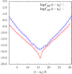
Figure 3: Time dependence of $C_{BB^{\dagger}}$ and $C_{JB^{\dagger}}$ on $16^{3}\!\times\!32$ lattice: reliable errorbars not yet available.

References

• [1] R. Frezzotti and G. C. Rossi, Phys. Rev. D92 (2015) 054505.
• [2] G. ’t Hooft, “Naturalness, Chiral Symmetry and Spontaneous Chiral Symmetry Breaking”, in “Recent Developments in Gauge Theories” (Plenum Press, 1980) - ISBN 978-0-306-40479-5.
• [3] D. Kaplan, Phys. Lett. B288, 342 (1992).
• [4] H. Neuberger, Phys. Lett. B417, 141 (1998).
• [5] I. Montvay and G. Münster, Quantum Fields on a Lattice, Cambridge Monographs on Mathematical Physics (Cambridge University Press, 1994): see in particular sections 4.3 and 4.4.
• [6] J. Bulava, P. Gerhold, K. Jansen, et al., ”Higgs-Yukawa Model in Chirally Invariant Lattice Field Theory,” Advances in High Energy Physics, vol. 2013, Article ID 875612, 24 pages, 2013.