Simultaneous longitudinal and transverse oscillation in an active filament

1 Introduction

Filaments support both longitudinal and transverse oscillations (see, Arregui, Oliver, and Ballester, 2012). The oscillations in the filaments can be used to diagnose the local plasma conditions and magnetic field by applying the principle of MHD seismology (see, Nakariakov and Verwichte, 2005; Andries, Arregui, and Goossens, 2005). These oscillations are broadly classified as large amplitude (Tripathi, Isobe, and Jain, 2009) and small amplitude (Oliver and Ballester, 2002) oscillations. Large amplitude transverse oscillations, where a filament oscillates as whole, are often associated with the disturbances coming from nearby flares (Ramsey and Smith, 1966; Isobe and Tripathi, 2006; Okamoto et al., 2004; Hershaw et al., 2011; Schmieder et al., 2013; Pant et al., 2015). In contrast, the large amplitude longitudinal oscillations are always found to be associated with small energetic events like a subflare at one leg of the filament (Jing et al., 2003), a small flare in a nearby active region (Jing et al., 2006; Vršnak et al., 2007; Li and Zhang, 2012) or jets (Luna et al., 2014). There have been several reports on large amplitude longitudinal oscillations (Jing et al., 2003, 2006; Vršnak et al., 2007; Luna and Karpen, 2012; Luna, Díaz, and Karpen, 2012; Zhang et al., 2012; Luna et al., 2014). Luna and Karpen (2012) developed a 1D self-consistent model which explained both restoring force and damping of large amplitude longitudinal oscillations. The model is analogous to an oscillating pendulum assuming the radius of curvature of magnetic dip as the length of the pendulum. Luna et al. (2014) used this model to explain the strong damping of large amplitude longitudinal oscillations observed in the filament threads. Recently, Luna et al. (2016) performed 2D non-linear time dependent MHD simulations where a magnetic field can get distorted in response to the mass loading. The authors have reported that a simple pendulum model can be used to characterise the large amplitude longitudinal oscillations even in a scenario where the magnetic field responds to the plasma motions.
Damping of oscillations have been observed in large amplitude transverse oscillations (Hershaw et al., 2011; Pant et al., 2015). Goossens, Andries, and Arregui (2006); Arregui et al. (2007) used seismology combining the damping time and period of oscillations in a consistent manner to estimate the magnetic field strength and inhomogeneity length scale in the coronal loops. Arregui et al. (2008) applied the same technique to the oscillating threads of a prominence. Pant et al. (2015) applied this technique to estimate magnetic field and inhomogeneity length scale of a filament as whole.
In addition to transverse oscillations, large amplitude longitudinal oscillations are also found to be damped (Luna and Karpen, 2012; Luna et al., 2014). Unlike transverse oscillations, that are now believed to be damped by the resonant absorption, damping mechanisms in longitudinal oscillations are not well understood. Several damping mechanisms have been proposed, e.g., energy leakage (Kleczek and Kuperus, 1969), dissipation (Tripathi, Isobe, and Jain, 2009) but these mechanisms are under debate. However, mass accretion due to the condensation of filament material (Luna and Karpen, 2012; Luna et al., 2014, 2016; Ruderman and Luna, 2016) is shown to be promising in explaining the damping of longitudinal oscillations in a filament. Recently, Ruderman and Luna (2016) have reported the evidence of strong damping of longitudinal oscillations in the filament threads that are modelled as a curved magnetic tube.
Shen et al. (2014) reported that an incoming shock wave can trigger longitudinal and transverse oscillations in the filaments depending on the interaction angle between the filament and the shock wave. Gilbert et al. (2008) has reported coexistence of two transverse oscillation modes, one in the plane of sky and other along the line of sight, in a filament in response to a Moreton wave. Both modes were perpendicular to the filament axis. In this work, we report a unique observation of the co-existence of large amplitude damped longitudinal oscillations and large amplitude damped transverse oscillations in an active region filament. The paper is organised as follows. In Section 2, we describe the observations. In Section 3 we discuss the methods of data analysis. We present the results in Section 4, which is followed by the discussion and conclusions in Section 5.

2 Observation

A M1.1 Class flare was observed by GOES satellite in an active region AR 11692 on March 15^th 2013. The flare was associated with a halo coronal mass ejection (CME). The flare created a global disturbance in the active region. The CME associated with the flare produced a shock wave. To observe shock fronts, we created running difference images of AIA 193 Å. The shock fronts are marked with red and green arrows in Figure shock_fig. It is evident from Figure shock_fig that the shock fronts are moving outward.

A filament was lying to the south-west of the active region as seen in H$\alpha$ images from NSO/GONG (Figure context). NSO/GONG provides full-disk observation of the Sun in 6563 Å (H$\alpha$). It has a pixel resolution of $\sim$ 1.07${}^{{}^{\prime\prime}}$and a cadence of 1 sec. The observational data used in this study are obtained from 06:00:54 UT to 10:22:54 UT. The flare started at 05:46:00 UT, peaked at 06:58:00 UT and ended at 08:35:00 UT as recorded in GOES catalogue. We note that just after the onset of the flare, oscillations were triggered in the filament.
Filaments consist of fine threads that are not often seen in GONG H$\alpha$ images due to its poor spatial resolution. Therefore, we use the images from the extreme ultraviolet (EUV) passbands of Atmospheric Imaging Assembly (AIA) onboard Solar Dynamic Observatory (SDO). AIA instrument provides almost simultaneous full-disk images of the Sun in seven EUV band. It has a spatial resolution of $1.3^{\prime\prime}$, pixel size of $0.6^{\prime\prime}$ and a cadence of 12 s (Lemen et al., 2012). We find that the filament consists of several threads that are seen more clearly in AIA 171 Å than any other EUV passbands of AIA. Therefore, we use AIA 171 Å  for further analysis. Moreover, we find that shortly after the oscillations started, the full disk images of the Sun were not available from 06:22:23 UT to 07:36:00 UT. Thus, the first cycle of oscillations is not seen in AIA 171 Å.
We overplot the contours of the filament as seen in GONG H$\alpha$ over the magnetogram obtained from Helioseismic and Magnetic Imager (HMI) onboard SDO (Figure hmi). We find that the filament lies over the region which separates the positive and the negative polarity. We note from the movie (available online) that at 06:11:59 UT, i.e before eruption, the filament material as enclosed in two different contours are part of the same filament (Pant et al., 2015, right panel of Figure 1).
By careful inspection of the H$\alpha$ images in the movie (available online), it appears that both longitudinal and transverse oscillations are present simultaneously in the filament. In the movie (available online), we mark the filament in AIA images with a green arrow. The transverse oscillations in the filament under study are already reported in Pant et al. (2015). In this paper, we focus on longitudinal oscillations at two parts of the filament adjacent to its two ends.

Figure 1.: Difference images of AIA 193 Å at four different time instances. Arrows in red and green represent the shock front.shock˙fig

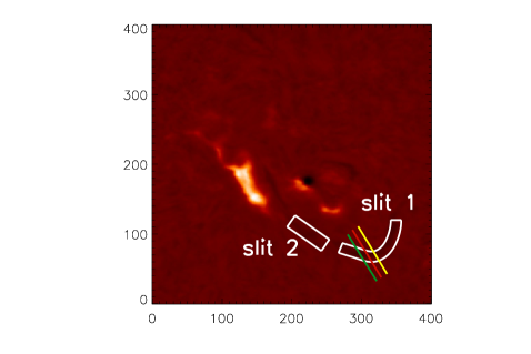
Figure 2.: NSO/GONG H$\alpha$ image of the filament lying at south-west of the active region AR 11692. Two broad artificial slices along the axis of the filament, used for generating x–t maps, are over plotted. Three artificial slits perpendicular to the axis of filament are overplotted in green, red and yellow, which were used in Pant et al. (2015) to investigate the transverse oscillations.context

Figure 3.: Left: GONG H$\alpha$ image. Right HMI magnetogram. Overplotted red contours outline the position of the filament.hmi

3 Data Analysis

3.1 GONG H$\alpha$

To investigate the longitudinal oscillations in GONG H$\alpha$ images, we place two artificial broad slices, slit 1 and slit 2 along the axis of the filament as shown in Figure context. The length (width) of the $1^{st}$ and the $2^{nd}$ slice is 130 pixel (15 pixel) and 60 pixel (20 pixel) respectively. The filament is oscillating in both transverse and longitudinal directions simultaneously. We choose broad slices so that the filament material remain inside the slices in spite of the transverse oscillations.

To further characterise the longitudinal oscillations in the filament, first we create a time-distance (x–t) map with time in x axis and distance along the slice in y axis for both slit 1 and slit 2. Intensity along each column of the x–t map is fitted with a Gaussian curve. The mean value and one sigma error of the intensity is estimated. Finally the x–t map is fitted with a damped sinusoidal function to investigate the oscillation characteristics. Since the filament is oscillating and the amplitude of the oscillations is decreasing with time, it can be fitted with a damped sinusoidal function (assuming the mass of the filament to be constant) and represented as (Aschwanden et al., 1999),

$$y(t)=c+A_{sin}sin(\omega t+\phi_{sin})e^{-t/\tau_{sin}},$$ (1)

where $c$ is a constant, $A_{sin}$ is the amplitude, $\tau_{sin}$ is the damping time, $\omega$ is the angular frequency, and $\phi_{sin}$ is the initial phase of sinusoidal function. The least square fitting is done using the function MPFIT.pro in Interactive Data Language (IDL) (Markwardt, 2009). It has been shown that if a filament accretes mass then the Bessel function describes the oscillations better than the damped sinusoid (Luna and Karpen, 2012). Therefore, we fit the x–t map using a damped zeroth order Bessel function of first kind, represented by

$$y(t)=c_{1}+A_{bes}J_{0}(\omega t+\phi_{bes})e^{-t/\tau_{bes}},$$ (2)

where $c_{1}$ is a constant, $A_{bes}$ is amplitude, $\omega$ is the angular frequency, $\tau_{bes}$ is the damping time, and $\phi_{bes}$ is the phase of the Bessel function.

3.2 AIA 171 Å

We repeat the analysis on AIA 171 Å  images but with only one artificial slice. The filament material at the position of slit 2 is not clearly seen in AIA 304, 171 and 193 Å  due to the presence of overlying post-flare loops (see movie).

4 Results

4.1 GONG H$\alpha$

The period, damping time and amplitude estimated from the fitting of a damped sinusoidal function represented by Equation (1) are summarized in Table table1. The period, damping time and amplitude estimated from the fitting of a damped zeroth order Bessel function of first kind represented by Equation (2) is summarized in Table table2. In the right panel of Figure xt, we overplot dashed green lines at three time instances. It is evident that both ends of the filament started oscillating in different phase. It is also worth noting that the oscillations started at different times in the two ends of the filament.

4.2 AIA 171 Å

The period of oscillation is found to be 57$\pm$3 min which is similar to the period estimated at the position of slit 1 in GONG H$\alpha$. The damping time is estimated to be 100 min which is larger as compared to the damping time estimated using slit 1 in GONG H$\alpha$ images. Amplitude of oscillation is found to be 10 Mm which is less than the amplitude measured in GONG H$\alpha$ images. The main reason of large damping time and smaller amplitude is that, first cycle of the oscillations is missed in AIA 171 Å images, therefore the oscillations start after 100 min as shown in Figure xt_aia (right panel). We note from Figure xt (top right panel) that the estimated damping time of oscillations and amplitude are strongly dependent on first cycle of the oscillations. If first cycle of oscillations is missed then the damping time will be longer and amplitude will be smaller. Another reason can be that the filament threads apparently merge and separate during the oscillations. This may be attributed to the fact that multiple threads are stacked along the line of sight, so if they are not moving in phase it may appear that they are merging and separating. This is probably also related to the presence of transverse oscillations because such effect is not reported in earlier studies (Luna and Karpen, 2012) where only longitudinal oscillations were present. Therefore, there is large uncertainty in choosing the thread that is associated with the oscillations (see right panel of Figure xt_aia). It is worth noting at this point that we did not fit damped Bessel function to AIA dataset because, as said above, the first cycle of oscillation is missed thus the Bessel function will not give the correct estimation of the damping time.

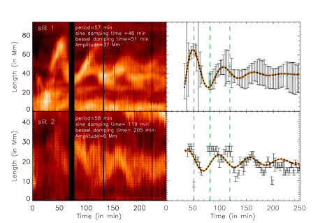
Figure 4.: Upper left panel shows the x–t map of slit 1. The thick black vertical strip represents the data gap between 07:07:54 Ut to 07:18:54 UT. The time period, amplitude and the damping time obtained from fitting is mentioned at the top of the plot. The lower left panel is same as upper left but for slit 2. In the upper right panel we plot the fitted damped sinusoidal curve with one sigma error bar. The lower right panel is same for the slice 2. Three vertical dashed lines over plotted at three time instances show that the oscillations started with different phases. The dotted black curve represents the best fit damped sinusoidal function while orange curve represents the damped Bessel functionxt

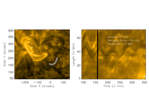
Figure 5.: The left panel shows the AIA 171 Å  image with artificial slice overplotted on the filament. The right panel represents the x–t map corresponding to the curve artificial slice shown in the left panel. The thick black vertical strip represents the data gap. Black curve represents the best fit sinusoidal function. The time period, amplitude and the damping time obtained from fitting is mentioned at the top.xt˙aia

4.3 Radius of curvature of magnetic dip

Filament material is supported by the magnetic fields against gravity. We use a simple pendulum model to estimate the oscillation parameters (Luna and Karpen, 2012). Assuming restoring force to be gravity, we get the following equation

$$\omega=\frac{2\pi}{P}=\sqrt{\frac{g_{0}}{R}},$$ (3)

where $g_{0}$ is the Sun’s surface gravity, $\omega$ is the oscillation frequency, $P$ is the period of oscillation and $R$ is the radius of curvature. Using Equation (3), the radius of curvature in GONG H$\alpha$ images is estimated to be $\sim$ 80 Mm and 85 Mm at the position of dip 1 (where $1^{st}$ slice is placed) and dip 2 (where $2^{nd}$ slice is placed; see, Figure context) respectively. Similarly, the radius of curvature at the location of dip 1 (see left hand panel of Figure xt_aia where artificial slice is placed) in AIA 171 Å is estimated to be 80 Mm.

4.4 Estimation of magnetic field strength

We calculate a lower limit of the magnetic field strength, assuming that magnetic stress is balanced by the weight of the filament material present in a dip (Luna and Karpen, 2012), using the following expression,

$$B(G)\geq 26\left(\frac{n_{e}}{10^{11}}\right)^{\frac{1}{2}}P,$$ (4)

where $B$ is the magnetic field, $n_{e}$ is the electron number density in cm^-3 and $P$ is the period of oscillation in hours. Here we use the typical value of electron number density $10^{11}$ cm^-3 as reported in Labrosse et al. (2010). Therefore, minimum magnetic field strength is estimated to be $\sim$ (25 $\pm$ 1) G both in dip 1 and dip 2 which is consistent with the typical values of the measured magnetic fields in the filaments (Labrosse et al., 2010; Mackay et al., 2010). Since the period of oscillation is estimated to be the same using AIA 171 Å, the estimated magnetic field strength remains unchanged.

4.5 Estimation of the Mass Accretion Parameter

In the model given by Luna and Karpen (2012), the damping of longitudinal oscillations in threads of the filaments is explained by the accretion of filament material. We calculate the mass accretion rate from the best fit parameters of the damped Bessel function (represented by Equation (2)), using the following relation (Luna et al., 2014),

$$\alpha=\frac{\omega m_{0}}{\phi_{bes}},$$

where, $m_{0}$ is the initial mass of filament, $\omega$ and $\phi_{bes}$ are the obtained from fitting of the damped Bessel function. The mass of a filament, $m_{0}$ can be calculated as $m_{0}=1.27m_{p}n_{e}\pi r^{2}L$, where $r$ and $L$ are the radius and the length of the thread of the filament. We take the typical radius of a filament thread to be 100 km as assumed in Luna et al. (2014). The length of the thread is estimated using x–t map as shown in Figure xt (top panel). As explained above, the artificial slit is placed along the length of the filament. Thus the extent of the brightness along each column of the x–t map gives an estimate of the length of the filament thread at a particular time instance. The length of the filament thread is measured at various time instances (i.e, along different columns) from the start to the end of the oscillations. Finally, we estimate the mean value of the length of the filament thread $\sim$ 23$\pm$ 7 Mm at the position of slit 1. Following the above procedure, the length of the filament thread at the position of slit 2 is estimated $\sim$ 10$\pm$4 Mm. It should be borne in mind that the estimation of the length of the filament thread at the position of slit 2 is uncertain because the oscillations are not clearly seen in the x–t maps as shown in the bottom panel of Figure xt. Under these assumptions we estimated the mass accretion rate at the position of slit 1 and 2 to be $\sim$ (51 $\pm$ 17 $\times$10⁶ kg hr^-1) and (192 $\pm$ 72 $\times$10⁶ kg hr^-1) respectively. The derived mass accretion rate at the position of slit 1 is comparable to those reported in earlier studies (Luna et al., 2014). It should be noted that at the position of slit 2 the mass accretion rate is higher while damping time is longer. One of the reasons for this discrepancy is the uncertainty in the fitting parameters. Since the mass accretion rate depends on the phase of the Bessel function which is estimated from the best fit parameters. Therefore, if the fitting of a function is not good then the value of phase will have large errors and thus can not be trusted.

Table 1.: Table of parameters of damped sine fittingtable1

Slit No.	Displacement amplitude	Period	Damping time	Velocity amplitude
	(in Mm)	(in min)	(in min)	(in km s-1)
slice 1	37$\pm$ 15	57$\pm$2	46$\pm$8	69$\pm$30
slice 2	6 $\pm$1	58$\pm$1	119.3$\pm$0.1	15$\pm$2

Table 2.: Table of parameters of modified Bessel function fittingtable2

Slit No.	Displacement amplitude	Period	Damping time	Velocity amplitude
	(in Mm)	(in min)	(in min)	(in km s-1)
slice 1	27$\pm$12	57$\pm$2	51$\pm$10	49$\pm$25
slice 2	6$\pm$2	58$\pm$1	204$\pm$38	11$\pm$4

4.6 Possibility of existence of both longitudinal and transverse wave from kink oscillation

In this subsection we investigate the possibility of the existence of both longitudinal and transverse oscillations driven by kink oscillations. We assume the filament as a cylinder embedded in a uniform plasma with low plasma $\beta$. Magnetic field is assumed to be constant inside the cylinder and the effects of gravity is ignored. The model set up is similar to the one described in Yuan and Van Doorsselaere (2016). To get the variation of thermodynamic quantities, linearized ideal MHD equations are used (see Ruderman and Erdélyi, 2009),

$$\rho=-\nabla.(\rho_{0}\xi),$$ (5)

$$\rho_{0}\frac{\partial^{2}\mathbf{\xi}}{\partial t^{2}}=-\nabla(p+\mathbf{b.B_{0}/\mu_{0}})+\frac{1}{\mu}[(\mathbf{B_{0}}.\nabla)\mathbf{b}+(\mathbf{b}.\nabla)\mathbf{B_{0}}],$$ (6)

$$\mathbf{b}=\nabla\times(\bf{\xi}\times\mathbf{B_{0}}),$$ (7)

$$p-C_{s}^{2}\rho=\mathbf{\xi}.(C_{s}^{2}\nabla\rho_{0}-\nabla p_{0}),$$ (8)

where $\xi$ is the Lagrange displacement vector, $\rho$, $p$ and b are perturbed quantities while $\rho_{0}$, $p_{0}$ and B₀ are unperturbed quantities. Neumann boundary conditions are assumed at $r=a$

$$[P_{T}]_{r=a}=0,$$

$$[\xi_{r}]_{r=a}=0$$

and Dirichlet boundary conditions are assumed at $r=0,\infty$

$$P_{T}|_{r=0}<\infty,$$

$$\xi^{2}|_{r=0}=\infty,$$

$$P_{T}|_{r\rightarrow\infty}=0,$$

$$\xi|_{r\rightarrow\infty}=0,$$

where $P_{T}$ is the total pressure.

For a filament, we define $\omega$, $\omega_{A}$, $\omega_{T}$ as kink, Alfvén and tube oscillation frequency respectively and the tube speed, $C_{T}$ is given by $C_{T}=\frac{C_{A}C_{s}}{\sqrt{C_{A}^{2}+C_{s}^{2}}}$ where $C_{A}=\frac{B_{0}}{\sqrt{\mu_{0}\rho_{0}}}$ is the Alfvén speed and $C_{s}=\sqrt{\frac{\gamma p_{0}}{\rho_{0}}}$ is the sound speed. $B_{0}$, $p_{0}$, $\rho_{0}$ are equilibrium magnetic filed, plasma pressure and plasma density respectively and $\mu_{0}$ is the magnetic permeability in free space. For kink mode (m=1), the total pressure perturbation, $P_{T1}=p+\mathbf{b.B_{0}/\mu_{0}}$, in the filament is assumed to be

$$P_{T1}=AR(r)\cos(\omega t)\sin(kz)\cos(\phi)$$ (9)

where $A$ is the amplitude of the total perturbed pressure. Since kink mode is not axisymmetric thus cos($\phi$) dependence is assumed. Substituting of Equation (9) into Equations (5-8) yields,

$$\frac{d^{2}P_{T1}}{dr^{2}}+\frac{dP_{T1}}{rdr}-(\kappa^{2}_{r}+\frac{1}{r^{2}})P_{T1}=0,$$ (10)

where

$$\kappa^{2}_{r}=\frac{(\omega_{s}^{2}-\omega^{2})(\omega_{A}^{2}-\omega^{2})}{(\omega_{s}^{2}+\omega_{A}^{2})(\omega_{T}^{2}-\omega^{2})}k^{2},$$ (11)

where $\omega_{s}^{2}=k^{2}C_{s}^{2}$. Equation (10) should also hold true for R(r). In this work we confine ourselves to the inside of the flux tube thus, on solving Equation (10) for R(r), we get,

$$R=J_{1}(|\kappa_{r}|r).$$

In cylindrical coordinates, $v_{r}$ is the perturbed velocity amplitude of the transverse oscillation and $v_{z}$ is the perturbed velocity amplitude of the longitudinal oscillation. Inside the cylinder the perturbed radial and axial component of velocity amplitude are defined as (see Yuan and Van Doorsselaere, 2016, for details),

$$v_{r}=-\frac{rdR}{Rdr}\sin(\omega t)\sin(kz)\cos(\phi)$$

and

$$v_{z}=-\frac{C_{T}^{2}}{C_{A}^{2}}kr\frac{\omega^{2}-\omega_{A}^{2}}{\omega^{2}-\omega_{T}^{2}}\sin(\omega t)\cos(kz)\cos(\phi).$$

Thus, axial to radial velocity amplitude ratio is given by the following expression,

$$\frac{v_{z}}{v_{r}}=k\frac{C_{T}^{2}}{C_{A}^{2}}\frac{R}{\frac{dR}{dr}}\frac{\omega^{2}-\omega_{A}^{2}}{\omega^{2}-\omega_{T}^{2}}cot(kz).$$ (12)

We take the length of slit 2 as length of the filament, which is estimated to be 90 Mm. The radius of the filament is estimated to be $\sim$ 1 Mm. It is important to note that here we assume the length of the flux tube (modelled as a filament) as the length of the slit covering the filament material because here we compare longitudinal oscillations with the transverse oscillations as reported by Pant et al. (2015), where authors assumed that filament was oscillating as a whole in the transverse direction. To estimate the ratio of the axial to radial velocity amplitude, we choose three slit positions as shown in green, red and yellow lines in Figure context, that were used by Pant et al. (2015). From observations, we find that the longitudinal velocity amplitude to the transverse velocity amplitude ratio at these locations are 3.92, 3.26 and 2.22 respectively. Using Equation (12), we estimate the ratio to be 4 $\cdot$ $10^{-4}$, 2 $\cdot$ $10^{-4}$ and 1 $\cdot$ $10^{-5}$ respectively assuming typical value of sound speed in chromosphere as 15 km s^-1, Alfvén speed in three slit positions as 82, 88 and 91 km s^-1 respectively and perturbation frequency (assumed to be equal to the kink oscillation frequency) to be 117, 124 and 128 km s^-1 respectively (see, Pant et al., 2015). It should be borne in mind that a linear analysis is presented here. Considering the observed displacement to be large, non-linear effects would become important. Therefore to model such events further studies are needed. Nevertheless, from above analysis, we note that it is almost impossible to detect longitudinal oscillation in low-$\beta$ plasma as a result of fast kink mode in our observation. Therefore, large amplitude longitudinal oscillations cannot be the kink mode.

5 Interaction of shock with filament

In this section, we explore the most likely mechanism for driving the longitudinal and transverse oscillations in a filament channel. Shen et al. (2014) reported that shock waves can interact with filaments in two possible geometries. If shock waves come such that the normal vector to the shock wave is perpendicular to the filament axis then a filament oscillates in the transverse direction. While if the shock wave interacts with a filament such that the normal vector of the shock wave is parallel to the filament axis then a filament oscillates in the longitudinal direction. Here we are proposing a more general scenario where a shock wave interacts obliquely with the filament such that the filament material oscillates in both transverse and longitudinal direction as revealed from our observations. The position of the shock fronts in our observations are clearly seen in Figure shock_fig. However, it should be borne in mind that from observations it is not straight forward to determine the direction of shock with respect to the filament because the filament is in close proximity of the active region and is associated with overlying loops that expand in response to the shock wave. This makes it extremely difficult to determine the orientation of the shock wave.

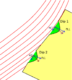
Figure 6.: A cartoon depicting the interaction of a shock wave with a filament. The filament has two magnetic dips, Dip 1 and Dip 2. The filament material is shown in green. The shock wave front is represented by red curves. The normal vector to shock wave front is shown in dark red. Arrows in blue represent the parallel and perpendicular component of the normal vector.cartoon

We depict this by a cartoon in Figure cartoon. We show that when a shock wave hit a filament obliquely, the normal vector to the wave front, $\hat{n}$ (shown in dark red), can be decomposed into perpendicular ($n_{\bot}$) and parallel ($n_{||}$) components as shown in Figure cartoon in blue. The component parallel to the filament axis triggers the longitudinal oscillations in the filament while the component perpendicular to the filament axis triggers the transverse oscillations in the filament. Thus the shock front interacts with the filament at dip 1 and displaces the filament material in both transverse and longitudinal direction. Similarly in dip 2 the shock front displaces the plasma in both transverse and longitudinal directions, but at a different time. With this schematic picture we can explain the different start time of longitudinal oscillation at two ends of the filament. However, with this scenario, one should expect the transverse oscillations to be present at the locations of both dips but transverse oscillations are only observed at the location of dip 1. It is worth noting that this is the simple geometry. In principle many parts of the shock wave can interact with the filament at different orientations and can excite different modes. Further studies are needed to confirm this.

6 Summary and Conclusions

In this work, we find the co-existence of longitudinal and transverse oscillations in an active region filament as observed by NSO/GONG H$\alpha$. The oscillations are triggered by the interaction of a shock wave with the filament. We find that the oscillations in two ends of the filament started with different phase but with almost similar period of oscillations. We note that the longitudinal oscillations at two slit positions started at different times (see, Figure xt) may be because the shock wave front interacts with the two parts of filament at different time instances. We depict it with a schematic diagram (see, Figure cartoon).

The damping time at the position of slit 1 is estimated to be 46 minute. This is a bit too strong as compared to the earlier reports (Tripathi, Isobe, and Jain, 2009) and comparable to what is reported in Luna et al. (2014). Luna and Karpen (2012) suggested that the mass accretion of the filament material is responsible for damping. We find mass accretion rate to be 51 $\pm$ 17 $\times$10⁶ kg hr^-1 at the position of slit 1 and 192 $\pm$ 72 $\times$10⁶ kg hr^-1 at the position of slit 2 which is comparable with the earlier reports (Luna et al., 2014). We performed the filament seismology and estimated the magnetic field strength at two dip locations. We estimated the lower limit of the magnetic field strength $\sim$ (25 $\pm$ 1) G at the location of both the slices which is consistent with typical values of measured magnetic field from observation (Mackay et al., 2010). We also calculate the radius of curvature of two magnetic dips of the filament as 80 Mm and 85 Mm for dip 1 and dip 2, respectively.

From our observations we exclude the possibility of existence of transverse and longitudinal oscillation simultaneously driven by a fast kink mode. Longitudinal oscillations due to kink wave may be present but their amplitude is far less as compared to the amplitude of the longitudinal oscillations observed in this case. Thus we believe that transverse and longitudinal oscillations exist independently in the filament under study.

Acknowledgement

We would like to thank the referee for his/her valuable comments which has improved the presentation of this article.

References

- Andries, Arregui, and Goossens (2005) Andries, J., Arregui, I., Goossens, M.: 2005, Determination of the Coronal Density Stratification from the Observation of Harmonic Coronal Loop Oscillations. ApJ 624, L57. DOI. ADS.
- Arregui, Oliver, and Ballester (2012) Arregui, I., Oliver, R., Ballester, J.L.: 2012, Prominence Oscillations. Living Reviews in Solar Physics 9, 2. DOI. ADS.
- Arregui et al. (2007) Arregui, I., Andries, J., Van Doorsselaere, T., Goossens, M., Poedts, S.: 2007, MHD seismology of coronal loops using the period and damping of quasi-mode kink oscillations. A&A 463, 333. DOI. ADS.
- Arregui et al. (2008) Arregui, I., Terradas, J., Oliver, R., Ballester, J.L.: 2008, Damping of Fast Magnetohydrodynamic Oscillations in Quiescent Filament Threads. ApJ 682, L141. DOI. ADS.
- Aschwanden et al. (1999) Aschwanden, M.J., Fletcher, L., Schrijver, C.J., Alexander, D.: 1999, Coronal Loop Oscillations Observed with the Transition Region and Coronal Explorer. ApJ 520, 880. DOI. ADS.
- Gilbert et al. (2008) Gilbert, H.R., Daou, A.G., Young, D., Tripathi, D., Alexander, D.: 2008, The Filament-Moreton Wave Interaction of 2006 December 6. ApJ 685, 629. DOI. ADS.
- Goossens, Andries, and Arregui (2006) Goossens, M., Andries, J., Arregui, I.: 2006, Damping of magnetohydrodynamic waves by resonant absorption in the solar atmosphere. Philosophical Transactions of the Royal Society of London Series A 364, 433. DOI. ADS.
- Hershaw et al. (2011) Hershaw, J., Foullon, C., Nakariakov, V.M., Verwichte, E.: 2011, Damped large amplitude transverse oscillations in an EUV solar prominence, triggered by large-scale transient coronal waves. A&A 531, A53. DOI. ADS.
- Isobe and Tripathi (2006) Isobe, H., Tripathi, D.: 2006, Large amplitude oscillation of a polar crown filament in the pre-eruption phase. A&A 449, L17. DOI. ADS.
- Jing et al. (2003) Jing, J., Lee, J., Spirock, T.J., Xu, Y., Wang, H., Choe, G.S.: 2003, Periodic Motion along a Solar Filament Initiated by a Subflare. ApJ 584, L103. DOI. ADS.
- Jing et al. (2006) Jing, J., Lee, J., Spirock, T.J., Wang, H.: 2006, Periodic Motion Along Solar Filaments. Sol. Phys. 236, 97. DOI. ADS.
- Kleczek and Kuperus (1969) Kleczek, J., Kuperus, M.: 1969, Oscillatory Phenomena in Quiescent Prominences. Sol. Phys. 6, 72. DOI. ADS.
- Labrosse et al. (2010) Labrosse, N., Heinzel, P., Vial, J.-C., Kucera, T., Parenti, S., Gunár, S., Schmieder, B., Kilper, G.: 2010, Physics of Solar Prominences: I Spectral Diagnostics and Non-LTE Modelling. Space Sci. Rev. 151, 243. DOI. ADS.
- Lemen et al. (2012) Lemen, J.R., Title, A.M., Akin, D.J., Boerner, P.F., Chou, C., Drake, J.F., Duncan, D.W., Edwards, C.G., Friedlaender, F.M., Heyman, G.F., Hurlburt, N.E., Katz, N.L., Kushner, G.D., Levay, M., Lindgren, R.W., Mathur, D.P., McFeaters, E.L., Mitchell, S., Rehse, R.A., Schrijver, C.J., Springer, L.A., Stern, R.A., Tarbell, T.D., Wuelser, J.-P., Wolfson, C.J., Yanari, C., Bookbinder, J.A., Cheimets, P.N., Caldwell, D., Deluca, E.E., Gates, R., Golub, L., Park, S., Podgorski, W.A., Bush, R.I., Scherrer, P.H., Gummin, M.A., Smith, P., Auker, G., Jerram, P., Pool, P., Soufli, R., Windt, D.L., Beardsley, S., Clapp, M., Lang, J., Waltham, N.: 2012, The Atmospheric Imaging Assembly (AIA) on the Solar Dynamics Observatory (SDO). Sol. Phys. 275, 17. DOI. ADS.
- Li and Zhang (2012) Li, T., Zhang, J.: 2012, SDO/AIA Observations of Large-amplitude Longitudinal Oscillations in a Solar Filament. ApJ 760, L10. DOI. ADS.
- Luna and Karpen (2012) Luna, M., Karpen, J.: 2012, Large-amplitude Longitudinal Oscillations in a Solar Filament. ApJ 750, L1. DOI. ADS.
- Luna, Díaz, and Karpen (2012) Luna, M., Díaz, A.J., Karpen, J.: 2012, The Effects of Magnetic-field Geometry on Longitudinal Oscillations of Solar Prominences. ApJ 757, 98. DOI. ADS.
- Luna et al. (2014) Luna, M., Knizhnik, K., Muglach, K., Karpen, J., Gilbert, H., Kucera, T.A., Uritsky, V.: 2014, Observations and Implications of Large-amplitude Longitudinal Oscillations in a Solar Filament. ApJ 785, 79. DOI. ADS.
- Luna et al. (2016) Luna, M., Terradas, J., Khomenko, E., Collados, M., de Vicente, A.: 2016, On the Robustness of the Pendulum Model for Large-amplitude Longitudinal Oscillations in Prominences. ApJ 817, 157. DOI. ADS.
- Mackay et al. (2010) Mackay, D.H., Karpen, J.T., Ballester, J.L., Schmieder, B., Aulanier, G.: 2010, Physics of Solar Prominences: II Magnetic Structure and Dynamics. Space Sci. Rev. 151, 333. DOI. ADS.
- Markwardt (2009) Markwardt, C.B.: 2009, Non-linear Least-squares Fitting in IDL with MPFIT. In: Bohlender, D.A., Durand, D., Dowler, P. (eds.) Astronomical Data Analysis Software and Systems XVIII, Astronomical Society of the Pacific Conference Series 411, 251. ADS.
- Nakariakov and Verwichte (2005) Nakariakov, V.M., Verwichte, E.: 2005, Coronal Waves and Oscillations. Living Reviews in Solar Physics 2. DOI. ADS.
- Okamoto et al. (2004) Okamoto, T.J., Nakai, H., Keiyama, A., Narukage, N., UeNo, S., Kitai, R., Kurokawa, H., Shibata, K.: 2004, Filament Oscillations and Moreton Waves Associated with EIT Waves. ApJ 608, 1124. DOI. ADS.
- Oliver and Ballester (2002) Oliver, R., Ballester, J.L.: 2002, Oscillations in Quiescent Solar Prominences Observations and Theory (Invited Review). Sol. Phys. 206, 45. DOI. ADS.
- Pant et al. (2015) Pant, V., Srivastava, A.K., Banerjee, D., Goossens, M., Chen, P.-F., Joshi, N.C., Zhou, Y.-H.: 2015, MHD Seismology of a loop-like filament tube by observed kink waves. Research in Astronomy and Astrophysics 15, 1713. DOI. ADS.
- Ramsey and Smith (1966) Ramsey, H.E., Smith, S.F.: 1966, Flare-initiated filamei it oscillations. AJ 71, 197. DOI. ADS.
- Ruderman and Luna (2016) Ruderman, M., Luna, M.: 2016, Damping of prominence longitudinal oscillations due to mass accretion. ArXiv e-prints. ADS.
- Ruderman and Erdélyi (2009) Ruderman, M.S., Erdélyi, R.: 2009, Transverse Oscillations of Coronal Loops. Space Sci. Rev. 149, 199. DOI. ADS.
- Schmieder et al. (2013) Schmieder, B., Kucera, T.A., Knizhnik, K., Luna, M., Lopez-Ariste, A., Toot, D.: 2013, Propagating Waves Transverse to the Magnetic Field in a Solar Prominence. ApJ 777, 108. DOI. ADS.
- Shen et al. (2014) Shen, Y., Liu, Y.D., Chen, P.F., Ichimoto, K.: 2014, Simultaneous Transverse Oscillations of a Prominence and a Filament and Longitudinal Oscillation of Another Filament Induced by a Single Shock Wave. ApJ 795, 130. DOI. ADS.
- Tripathi, Isobe, and Jain (2009) Tripathi, D., Isobe, H., Jain, R.: 2009, Large Amplitude Oscillations in Prominences. Space Sci. Rev. 149, 283. DOI. ADS.
- Vršnak et al. (2007) Vršnak, B., Veronig, A.M., Thalmann, J.K., Žic, T.: 2007, Large amplitude oscillatory motion along a solar filament. A&A 471, 295. DOI. ADS.
- Yuan and Van Doorsselaere (2016) Yuan, D., Van Doorsselaere, T.: 2016, Forward Modeling of Standing Kink Modes in Coronal Loops. I. Synthetic Views. ApJS 223, 23. DOI. ADS.
- Zhang et al. (2012) Zhang, Q.M., Chen, P.F., Xia, C., Keppens, R.: 2012, Observations and simulations of longitudinal oscillations of an active region prominence. A&A 542, A52. DOI. ADS.