Auxiliary variables for nonlinear equations with softly broken symmetries

Abstract

General methods of solving equations deal with solving $N$ equations in $N$ variables and the solutions are usually a set of discrete values. However, for problems with a softly broken symmetry these methods often first find a point which would be a solution if the symmetry were exact, and is thus an approximate solution. After this, the solver needs to move in the direction of the symmetry to find the actual solution, but that can be very difficult if this direction is not a straight line in the space of variables. The solution can often be found much more quickly by adding the generators of the softly broken symmetry as auxiliary variables. This makes the number of variables more than the equations and hence there will be a family of solutions, any one of which would be acceptable. In this paper we present a procedure for finding solutions in this case, and apply it to several simple examples and an important problem in the physics of false vacuum decay. We also provide a Mathematica package that implements Powell’s hybrid method with the generalization to allow more variables than equations.

1 Introduction

Numerical methods of solving equations are one of the most important topics in numerical analysis. There is a plethora of techniques which each is adequate for specific sets of problems. For examples refer to [1] and references therein. All techniques attempt to successively improve some guess for the variable values.

The best-known of these is Newton’s method (also called Newton-Raphson), which works by linearizing the equations around the current guess and solving the linearized problem. It converges very rapidly when it gets near the solution, but if it is not close to the solution it can take large steps in unhelpful directions that make the next guess worse than the previous one.

An alternative is to attempt to minimize the sum of the squares of a set of functions by descending the gradient of the total error. This method improves the solution at each step but can be very slow. There are also hybrid methods which combine these two [2].

The general techniques of solving equations involve solving a set of $N$ equations of $N$ variables where the solution is usually a discrete set of vectors. However, for problems with softly broken symmetries, as described below, these techniques can be very slow, sometimes so slow that the solution cannot be found. The problem is that there can be a complicated manifold of approximate solutions related by the broken symmetry. Once the technique finds one such solution, almost every possible step will make the error much worse. Any technique that depends on making progress in the sense of decreasing the error will be forced to take a very large number of tiny steps.

To solve such problems we propose adding auxiliary variables which are the generators of the softly broken symmetry, without adding new equations. The idea of adding variables for solving equations is not new, but it is usually accompanied by adding an equal number of equations. In our method we add new variables only.

This paper is organized as follows. In Section 2 we lay out the formalism for adding new variables. In Section 3 we present two simple examples with softly broken symmetries and the reason for adding new unknowns. In Section 4 we present a specific theoretical physics problem that can be solved this way. In Section 5 we briefly introduce a Mathematica package for Powell’s hybrid method and we conclude in Section 6

2 Problem, formalism and algorithm

Suppose one wants to solve a set of equations in the form

$$f_{i}(\mathbf{x})=0~{},\qquad i=1,\ldots,N~{},$$ (1)

where $\mathbf{x}$ has $N$ elements, using an equation solver, which could use Newton, gradient or hybrid methods. This always starts by choosing an initial guess for the solution $\mathbf{x}_{0}$ and taking steps according to some rule for approaching the solution. Of course the initial guess will not be the solution and hence the functions $f_{i}(\mathbf{x}_{0})$’s do not vanish. The goal of taking a step is to find a new set of points $\mathbf{x}_{1},\mathbf{x}_{2},\ldots,\mathbf{x}_{I}$ in such a way that the values of the $f_{i}$ in each step get closer to zero, at least in some aggregate sense.

Let us define the error as

$$\mathop{\mathrm{error}}(\mathbf{x})=\left(\sum_{i=1}^{N}{f_{i}(\mathbf{x})^{2}}\right)^{1/2}~{}.$$ (2)

In some cases, for example Fig. 1 below, the geometry the of error function is such that there are narrow valleys, which makes the steps very small without much progress in each step. In this case the error along the valley decreases very slowly because the error function has an approximate rotational symmetry. If one can add a variable which allows the solver move to quickly along the valley, the generator of the rotation in the case of Fig. 1, the solution can be found much more easily. Notice that this is a very simple version of the problem. Real problems can have valleys which have sharp turns, and for more than two variables the geometry can be much more complicated.

Suppose we now add extra variables $\mathbf{y}=\{y_{1},y_{2},\ldots,y_{K}\}$ and extend our functions $f_{i}(\mathbf{x})$ to some $g_{i}(\mathbf{x},\mathbf{y})$ such that $g_{i}(\mathbf{x},0)=f_{i}(\mathbf{x})$. It is now possible to move in new directions given by $\mathbf{y}$. If these variables have been chosen well, the solver will be able to take large steps in the new directions that quickly reduce the error and lead to a solution. In particular, if the valley of approximate solutions is straight, or at least close to straight, in the new variables, then the solver can make rapid progress. We show examples of this phenomenon in Sections 3 and 4.

Of course, since we add variables without adding constraints, the solution is not unique. For each solution of $f_{i}(\mathbf{x})=0$ there will be a $K$-dimensional family of solutions to $g_{i}(\mathbf{x},\mathbf{y})=0$. When the process succeeds, we have some solution $\{\mathbf{x},\mathbf{y}\}$, and we need to get from there to the solution of the original problem $f_{i}(\mathbf{x})=0$. But this is straightforward if the $\mathbf{y}$ are the generators of a symmetry. We can solve the original problem by simply applying the symmetry transformation to the $\mathbf{x}$ that we found.

We now present an algorithm for finding a solution of $N$ equations of $N+K$ variables using Powell hybrid techniques. Powell’s hybrid (or “dogleg”) method [2] takes steps which are a combination of the step recommended by Newton’s method and a step in the direction that most rapidly reduces $\mathop{\mathrm{error}}(\mathbf{x})$, i.e., the negative of the gradient of $\mathop{\mathrm{error}}(\mathbf{x})$. In the gradient case, the procedure is unaffected by additional variables. We simply have a scalar function of $N+K$ variables whose gradient we descend.

The application of Newton’s method is slightly more complicated. Newton’s method consists of linearizing the equations around some point $\mathbf{x}$ and solving the linearized equations. With $N$ equations in $N+K$ variables, there will be a $K$-dimensional subspace of solutions. In this case, we choose the solution which is nearest to the current guess in the Euclidean metric on the $N+K$ variables. This is straightforwardly determined by singular value decomposition of the rectangular Jacobian.

The steps chosen by gradient methods depend on the scaling of the variables (and also of the functions). Such methods try to find small steps in the space of variables that will lead to large improvements in the error. This feature can be used to control how much the solver tries to make use of the additional variables. If an additional variable is multiplied by some factor $s>1$ before being used in the function evaluation, the solver will give higher weight by factor $s$ to changes produced by this variable, and will be thus more likely to exploit that additional variable to simplify the problem.

The unmodified Newton’s method is invariant under rescaling of the variables (and the functions), because that doesn’t change the solution to the linearized problem. However, the modified method here chooses the closest point in the subspace of solutions. The factor $s$ increases the effect of the additional variable, so the change in it to achieve the same result is smaller. Thus increasing $s$ causes the modified Newton’s method to choose a solution whose differences are more due to the affected variable and less to the others.

3 Simple examples

In this section we present two problems with a softly broken symmetry and show the progress made by adding a new variable.

3.1 Softly broken rotational symmetry

We start from a very easy problem to demonstrate the main idea behind our proposal. Consider the functions

$$f_{1}(x,y) = x^{2}+y^{2}-a^{2}~{},$$

$$f_{2}(x,y) = bx~{},$$ (3)

for some parameters $a$ and $b$. We want to find $x$ and $y$, such that $f_{1}=f_{2}=0$. The solution is $y=\pm a$ and $x=0$, but we suppose we don’t know that and are trying to find the solution numerically. In the top panel of Fig. 1, we plot the

Figure 1: Top, the error as a function of $x$ and $y$ for the functions defined in (3.1) with $a=10$ and $b=1$. The problem has an approximate rotational symmetry. To see the breakdown of the symmetry on the right panel we zoomed in on the valley, which is slanted. The hybrid solver takes many small steps before finding the solution. On the bottom left panel we show the path that the hybrid solver took without an extra variable. On the right we show the path in $x$ and $y$ taken when we use the extra variable $\theta$. In this case, the solver takes steps in $x^{\prime}$, $y^{\prime}$, and $\theta$, but we graph the points $x$ and $y$ given by (3.1). In both cases the starting guess is $(-12\cos(\pi/8),12\sin(\pi/8))$. The left panel took 14 steps and the right only 5 steps. We see in the next figure that smaller $b$ increases the number of steps rapidly.

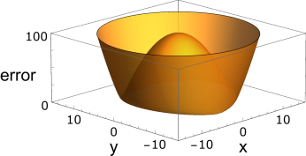
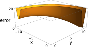
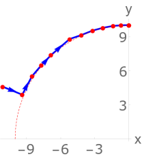
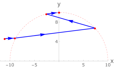
error for this set of equations with $a=10$ and $b=1$, as a function of the variables $x$ and $y$. The upper right panel shows a magnified picture of the curving and slanted valley. In the lower left of Fig. 1, we show the 14 steps taken by Powell’s method to find the solution.

Now let us introduce an extra variable which allows rotation, the broken symmetry. Instead of using $x$ and $y$ and variables, we use $x^{\prime}$, $y^{\prime}$, and $\theta$, with $x$ and $y$ given by

$$x = x^{\prime}\cos\theta+y^{\prime}\sin\theta~{},$$

$$y = -x^{\prime}\sin\theta+y^{\prime}\cos\theta~{}.$$ (4)

Our functions thus become

$$f_{1}(x,y) = x^{\prime 2}+y^{\prime 2}-a^{2}~{},$$

$$f_{2}(x,y) = b(x^{\prime}\cos\theta+y^{\prime}\sin\theta)~{}.$$ (5)

Now there will be an infinite number of solutions. For each value of $\theta$, there will be a solution $x^{\prime}$ and $y^{\prime}$. We can recover the values of $x$ and $y$ using (3.1). As shown in the lower right panel of Fig. 1 this problem is now solved in 5 steps.

In Fig. 2

Figure 2: The steps taken by the solver for the example presented in (3.1) for $a=10$ and $b=10^{-3}$. Now the rotational symmetry is broken very softly. Left shows the steps taken without the extra variable and right with an extra variable that generates the broken symmetry. In both cases the starting guess is $(-12\cos(\pi/8),12\sin(\pi/8))$. The left panel took 537 steps and the right only 5 steps.

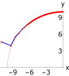
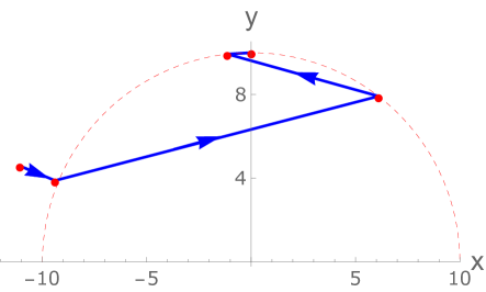
we show the path our solver took for $a=10$ and $b=10^{-3}$. The symmetry here is broken softly, so there is not much of a slant in the valley. If one uses a hybrid or gradient solver it takes a large number of steps to find the solution. For example Powell’s method took 537 steps, mostly creeping slowly along the valley, whereas with $\theta$ the solution can still be found in 5 steps.

This particular problem is rather trivial. Instead of adding a variable one could simply work in polar coordinates, which manifest the symmetry, and get the solution right away. This is possible because one can easily parameterize the remaining degree of freedom after the symmetry has been factored out.

One also can solve this problem by using a pure Newton method. Since one of the equations is linear, Newton’s method will solve it exactly in every step by jumping to some point on the $y$ axis. Newton’s method does not care about rescaling the equations and hence the smallness of $b$ is not important and the symmetry is not broken softly.

In the next sections we present two other problems where there is no obvious change of coordinate and the Newton technique does not necessarily work well.

3.2 Softly broken translational symmetry

In this section we present a problem where the correct parameterization is not as trivial as the previous one. Suppose we have some functions $f(x)$ and $g(x)$, chosen from families of similar functions, and we consider the function given by

$$F(x)=\left\{\begin{array}[]{ll}f(x)&f(x)<0~{},\\ g(x)&g(x)\geq 0~{}.\end{array}\right.$$ (6)

Here $f(x)$ and $g(x)$ are monotonically increasing functions. That to say that $F$ follows $f$ from $x=-\infty$ until $f(x)$ reaches 0, and $g$ from $x=\infty$ toward smaller $x$ until $g(x)$ reaches 0. To have a well-defined function, we would like $f(x)$ and $g(x)$ to reach 0 at the same point, and to have a $C^{1}$ function we would like the derivatives of $f$ and $g$ to match also at this point.

Our $f$ and $g$ will be chosen from the following classes of functions,

$$f(x) = ae^{x}+\epsilon e^{2x}-1~{},$$

$$g(x) = 1-be^{-(1+\epsilon)x}~{}.$$ (7)

where $a$ and $b$ specify which functions we chose and $\epsilon$ is a fixed small parameter.

To have a problem where the symmetry is easily shown, rather than specifying $a$ and $b$ we will specify that $F$ takes on a given value $F_{1}<0$ at a point $x_{1}$ and similarly a given value $F_{2}>0$ at a given point $x_{2}$. We will then attempt to vary $F_{1}$ and $F_{2}$ to find a well-defined $C^{1}$ function F.

First we explain the broken symmetry. If $\epsilon=0$, we have

$$f(x) = ae^{x}-1$$ (8)

$$g(x) = 1-be^{-x}~{}.$$ (9)

We want the two functions to join (vanish) at some $x_{0}$. For each value $x_{0}$ in the interval $(x_{1},x_{2})$ there will be a solution in the form

$$f(x_{1}) = e^{x_{1}-x_{0}}-1~{},$$ (10)

$$g(x_{2}) = 1-e^{x_{0}-x_{2}}~{}.$$ (11)

Hence the values of $F_{1}$ and $F_{2}$ only depend on $x_{1}-x_{2}$ and are invariant under a shift in these two numbers.

The terms which include $\epsilon$ break this symmetry softly and there will be unique values for $F_{1}$ and $F_{2}$ which make the function smooth. But because $\epsilon$ is small, it is difficult to find the correct values once we find some which solve the $\epsilon=0$ problem.

We now choose $x_{1}=-5$, $x_{2}=1$, and $\epsilon=10^{-3}$. Without adding an extra variable it took 299 steps for the solver to find $F_{1}$ and $F_{2}$. However, because we know the broken symmetry is translation, we simply allow for a shift in the values of $x$ by changing the equations to

$$f(x) = ae^{x-s\delta}+\epsilon e^{2(x-s\delta)}-1~{},$$ (12)

$$g(x) = 1-be^{-(1+\epsilon)(x-s\delta)}~{}.$$ (13)

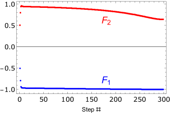
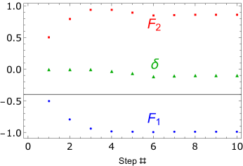
Because we are using a hybrid solver which is sensitive to the scaling of variables, we shifted by $s\delta$ with $s=10$ to encourage the solver to make use of $\delta$. Now there will be an infinite set of solutions $\{F_{1},F_{2},\delta\}$. After finding one such solution, we recover the original values of $F_{1}$ and $F_{2}$, by evaluating (12) at $x_{1}+s\delta$ and (13) at $x_{2}+s\delta$. With $\delta$ added, it took only 10 steps for the solver to find the solution. We show the steps that the solver took for this problem in Fig. 3.

In the next section we present an important physics problem which we solved in much more generality in [3] .

Figure 3: Left, the values of $F_{1}$ (blue circles) and $F_{2}$ (red squares) at steps taken by solver before finding the solution. Right, the same but this time an extra variable $\delta$ (green triangles) is added. The solution was found in 10 steps.

4 Tunneling in field theories

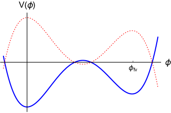
Problems of differential equations with boundary conditions at a specific point are commonplace in physics. One important examples is the equations used for calculation of cosmological phase transitions. Here we explain the problem briefly. The details can be found in [4]. In Fig. 4 we present a potential which has a metastable (false) minimum at $\phi_{f}$ and a stable (true) minimum at $\phi_{t}=0$. Finding the lifetime of this metastable minimum is tantamount to finding the solution of the differential equation

$$\phi^{\prime\prime}(r)+\frac{3}{r}\phi^{\prime}(r)=\frac{\partial U}{\partial\phi}~{},$$ (14)

with two boundary conditions,

$$\phi^{\prime}(0)=0~{},\qquad\phi(\infty)=\phi_{f}~{}.$$ (15)

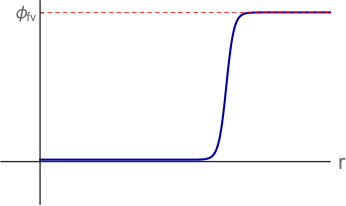
This is the same as the motion of a particle in the upside down potential shown in the red dotted graph in Fig. 4, under the influence of a velocity dependent friction given by $-3\phi^{\prime}(r)/r$. The standard technique is guessing $\phi(0)$ such that after evolving the fields it approaches $\phi_{f}$ . The field profile that solves this equation is shown in the right panel of Fig. 4. It is easy to see that this problem always allows a solution. If one chooses the value $\phi(0)$ very close to $\phi_{t}$ the field does not have any significant change until $r$ gets large. But then the friction term is negligible and the “energy” is conserved and it passes $\phi_{f}$. On the other hand if one chooses $\phi(0)$ such that $U(\phi(0))<\phi_{f}$, the particle can never reach $\phi_{f}$. The boundary between these two is the correct solution that asymptotes to $\phi_{f}$ at infinite $r$.

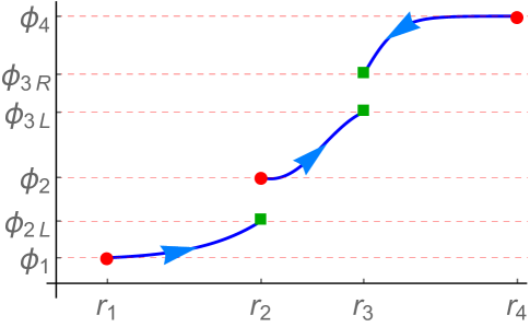
Generalization of this method to more than one field dimension done in [3] requires a different technique which is called “multi-interval shooting”. This method with 3 intervals is shown in Fig. 5. One guesses the value of the field at $r_{1}$ and $r_{4}$ and the value of the field and its derivative at $r_{2}$. We denoted these as $\{\phi_{1},\phi_{2},\phi^{\prime}_{2},\phi_{4}\}$. Having these and using analytic solutions near the true and false minima one can evolve the field equation (14) along the blue curve. The goal is finding the correct values of $\{\phi_{1},\phi_{2},\phi^{\prime}_{2},\phi_{4}\}$ such that the field and its derivative are continuous at $r_{2}$ and $r_{3}$. This creates a system of four equation of four variables. If not for the middle (friction) term in (14) and the fact that $\phi(0)$ is small but nonzero, it would possess a translational symmetry. Neglecting these two, if $\phi(r)$ satisfied the equations of motion and the boundary conditions, $\phi(r+\delta)$ would satisfy the same equations.

For the simple potential

$$U(\phi)=0.2\phi-2\phi^{2}+\phi^{4}~{},\quad\phi_{t}\approx-1.024~{},\quad\phi_{f}\approx 0.9740~{},$$ (16)

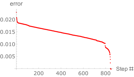
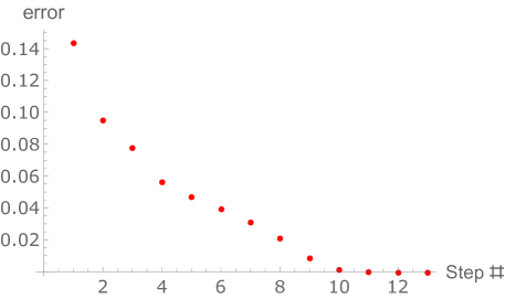
it took the hybrid solver 851 steps to find the solution. We chose the values of $\{r_{1},r_{2},r_{3},r_{4}\}=\{12.82,14.03,15.23,16.43\}$ using an analogy with the thin-wall solution. Because the softly broken symmetry is translation, when we specified the values of the field and derivative at $\{r_{1}+\delta,r_{2}+\delta,r_{3}+\delta,r_{4}+\delta\}$ instead of $\{r_{1},r_{2},r_{3},r_{4}\}$, allowing the solver to exploit the symmetry, the hybrid solver could find the solution in 12 steps. Most of the steps were taken in the “valley” which corresponds to a rigid shift of the profile $\phi(r)$. This is similar to the previous cases where the solver does not make much progress in each step as it moving along the “valley”. In Fig. 6 we show the change of error with and without adding the auxiliary variable $\delta$.

Figure 4: Left panel, a potential with two minima at $\phi_{t}=0$ and $\phi_{f}$ in solid blue and the upside down potential as the dotted red graph.. The minimum at $\phi_{f}$ is a metastable minimum and can tunnel quantum mechanically to the other minimum. Right panel, the solution to the field equation.

Figure 5: An illustration of multi-shooting method. One has to adjust the values of $\{\phi_{1},\phi_{2},\phi^{\prime}_{2},\phi_{4}\}$ and evolve the field equations (14) along the blue curves such that the field and its derivative are continuous at $r_{2}$ and $r_{3}$. This produces a system of four equations of four variables.

Figure 6: Left, the change of error after each step taken without adding an auxiliary variable and right the same when including $\delta$ for the potential in (16) in order to solve (14).

5 Powell-Hybrid package

We include with this paper a Mathematica code developed by one of us (K.D.O.), for the solution of simultaneous nonlinear equations using Powell’s hybrid method [2]. This code include the extension described here for solving $N+K$ equations in $N$ variables. However, it handles only problems where the Jacobian can be computed analytically. Powell [2] also includes a method for approximating the Jacobian using, mainly, the successive function evaluations, but we did not implement that.

The code and a manual for using it can be downloaded fromhttp://cosmos.phy.tufts.edu/Powell. This code is the same one used in [3].

6 Conclusion

In this paper we describe a new method for solving equations with a softly broken symmetry. The broken symmetry makes it very difficult for the solver to make progress towards minimizing the error in the desired equations. The error as a function of the variables usually has narrow valleys where moving along these valleys does not make large improvement. As a result the steps that the solver takes are small and it takes a very large number of steps for the solver to converge on the solution.

We introduced a method where one adds a set of auxiliary variables which are the generators of the softly broken symmetry. Adding these variables makes the solver take large steps in the direction along the valley and hence converges very quickly. Our method may be applicable beyond the theories with softly broken symmetries. We believe whenever such a valley is present adding variables which make the solver move in the proper direction makes converging much faster and the basin of attraction larger. However, for general valleys which are not the results of broken symmetries it may not be easy to identify the correct auxiliary variables to be added. For this reason we only mentioned these cases which we know the auxiliary variables must generate the broken symmetry. These techniques will be much more powerful and versatile if one can find a systematic way to determine the needed auxiliary variables.

7 Acknowledgement

This work was supported in part by the National Science Foundation [grant number PHY-1518742].

References

- [1] William H. Press, Saul A. Teukolsky, William T. Vetterling, and Brian P. Flannery. Numerical Recipes 3rd Edition: The Art of Scientific Computing. Cambridge University Press, New York, NY, USA, 3 edition, 2007.
- [2] M. J. D. Powell. A hybrid method for nonlinear equations. In Philip Rabinowitz, editor, Numerical methods for nonlinear algebraic equations, chapter 6, pages 87–114. Gordon and Breach Science Publishers, New York, 1970.
- [3] Ali Masoumi, Ken D. Olum, and Benjamin Shlaer. Efficient numerical solution to vacuum decay with many fields. 2016.
- [4] Sidney R. Coleman. The Fate of the False Vacuum. 1. Semiclassical Theory. Phys.Rev., D15:2929–2936, 1977.