Return probability and recurrence for the random walk driven by two-dimensional Gaussian free field

Abstract.

Given any $\gamma>0$ and for $\eta=\{\eta_{v}\}_{v\in\mathbb{Z}^{2}}$ denoting a sample of the two-dimensional discrete Gaussian free field on $\mathbb{Z}^{2}$ pinned at the origin, we consider the random walk on $\mathbb{Z}^{2}$ among random conductances where the conductance of edge $(u,v)$ is given by $\mathrm{e}^{\gamma(\eta_{u}+\eta_{v})}$. We show that, for almost every $\eta$, this random walk is recurrent and that, with probability tending to 1 as $T\to\infty$, the return probability at time $2T$ decays as $T^{-1+o(1)}$. In addition, we prove a version of subdiffusive behavior by showing that the expected exit time from a ball of radius $N$ scales as $N^{\psi(\gamma)+o(1)}$ with $\psi(\gamma)>2$ for all $\gamma>0$. Our results rely on delicate control of the effective resistance for this random network. In particular, we show that the effective resistance between two vertices at Euclidean distance $N$ behaves as $N^{o(1)}$.

¹ Department of Mathematics, UCLA, Los Angeles, California

² Center for Theoretical Study, Charles University, Prague, Czech Republic

³ Statistics Department, Wharton, University of Pennsylvania, Philadelphia, Pennsylvania

⁴ Institut des Hautes Études Scientifiques, Bures-sur-Yvette, France

1. Introduction

Let $\eta=\{\eta_{v}\}_{v\in\mathbb{Z}^{2}}$ denote a sample of the discrete Gaussian free field (GFF) on $\mathbb{Z}^{2}$ pinned to 0 at the origin. Explicitly, $\{\eta_{v}\}_{v\in\mathbb{Z}^{2}}$ is a centered Gaussian process such that

$$\eta_{0}=0\quad\text{\rm and}\quad\mathbb{E}(\eta_{u}\eta_{v})=G_{\mathbb{Z}^{2}\setminus\{0\}}(u,v)\,\text{\rm\ for all }\,u,v\in\mathbb{Z}^{2}\,,$$ (1.1)

where $G_{\mathbb{Z}^{2}\setminus\{0\}}(u,v)$ is the Green function in $\mathbb{Z}^{2}\setminus\{0\}$; i.e., the expected number of visits to $v$ for the simple random walk on $\mathbb{Z}^{2}$ started at $u$ and killed upon reaching the origin. For $\gamma>0$ and conditional on the sample $\eta$ of the GFF, let $\{X_{t}\}_{t\geq 0}$ be a discrete-time Markov chain with transition probabilities given by

$$p_{\eta}(u,v):=\frac{\mathrm{e}^{\gamma(\eta_{v}-\eta_{u})}}{\sum_{w:|w-u|_{1}=1}\mathrm{e}^{\gamma(\eta_{w}-\eta_{u})}}\mathbf{1}_{|v-u|_{1}=1}\,,$$ (1.2)

where $|\cdot|_{1}$ denotes the $\ell^{1}$-norm on $\mathbb{Z}^{2}$. We will write $P_{\eta}^{x}$ for the law of the above random walk such that $P_{\eta}^{x}(X_{0}=x)=1$ and use $E^{x}_{\eta}$ to denote the corresponding expectation. We also write $\mathbb{P}$ for the law of the GFF and use $\mathbb{E}$ (as above) to denote the expectation with respect to $\mathbb{P}$.

The transition kernel $p_{\eta}$ depends only on the differences $\{\eta_{x}-\eta_{y}\colon x,y\in\mathbb{Z}^{2}\}$ whose law is, as it turns out, invariant and ergodic with respect to the translations of $\mathbb{Z}^{2}$. (Thanks to the explicit control of correlation decay, the law is actually readily shown to be even strongly mixing.) The Markov chain $\{X_{t}\}_{t\geq 0}$ is thus an example of a random walk in a stationary random environment. The main conclusion we prove about this random walk is then:

Theorem 1.1.

For each $\gamma>0$ and each $\delta>0$,

$$\lim_{T\to\infty}\,\mathbb{P}\Bigl{(}\mathrm{e}^{-(\log T)^{1/2+\delta}}T^{-1}\leq P_{\eta}^{0}(X_{2T}=0)\leq\mathrm{e}^{(\log T)^{1/2+\delta}}T^{-1}\Bigr{)}=1\,.$$ (1.3)

Furthermore, $\{X_{t}\}_{t\geq 0}$ is recurrent for $\mathbb{P}$-almost every $\eta$.

The transition probabilities $p_{\eta}$ are such that the walk prefers to move along the edges where $\eta$ increases; the walk is thus driven towards larger values of the field. This has been predicted (e.g., in [19, 20]) to result in a subdiffusive behavior. We prove a version of subdiffusivity for the expected exit time from large balls:

Theorem 1.2.

Let $\tau_{B(N)^{\text{\rm c}}}$ denote the first exit time of $\{X_{t}\colon t\geq 0\}$ from the box $B(N):=[-N,N]^{2}\cap\mathbb{Z}^{2}$. For each $\delta>0$, we then have

$$\lim_{N\to\infty}\mathbb{P}\Bigl{(}N^{\psi(\gamma)}\mathrm{e}^{-(\log N)^{1/2+\delta}}\leq E_{\eta}^{0}\tau_{B(N)^{\text{\rm c}}}\leq N^{\psi(\gamma)}\mathrm{e}^{(\log N)^{1/2+\delta}}\Bigr{)}=1\,,$$ (1.4)

where

$$\psi(\gamma):=\begin{cases}2+2(\gamma/\gamma_{\text{\rm c}})^{2},\qquad&\text{\rm if }\gamma\leq\gamma_{\text{\rm c}}:=\sqrt{\pi/2},\\[2.84526pt] 4\gamma/\gamma_{\text{\rm c}},\qquad&\text{\rm otherwise}.\end{cases}$$ (1.5)

The bounds on the expected hitting time indicate that $|X_{T}|$ should scale as $T^{\frac{1}{\psi(\gamma)}+o(1)}$ for large $T$. Although we expect this to be true, we have so far only been able to prove a corresponding lower bound:

Theorem 1.3.

For $\mathbb{P}$-almost every $\eta$ and each $\delta>0$,

$$\,P_{\eta}^{0}\Bigl{(}|X_{T}|\geq\mathrm{e}^{-(\log T)^{1/2+\delta}}T^{\frac{1}{\psi(\gamma)}}\Bigr{)}\,\underset{T\to\infty}{\longrightarrow}\,1\quad\text{\rm in probability},$$ (1.6)

where $\psi(\gamma)$ is as in (1.5).

We note that Theorems 1.2 and 1.3 are consistent with the predictions in [19, 20] for general log-correlated fields. In particular, (1.6) confirms the prediction for the diffusive exponent of the walk from [19, 20] as a lower bound. The reason why the bounds in (1.4) are not sufficient is that we do not know whether $\tau_{B(N)^{\text{\rm c}}}$ scales with $N$ proportionally to its expectation. A full proof of subdiffusive behavior thus remains elusive.

The technical approach that makes our analysis possible stems from the following simple rewrite of the transition kernel achieved by multiplying both the numerator and the denominator in (1.2) by $\mathrm{e}^{2\gamma\eta_{u}}$,

$$p_{\eta}(u,v)=\frac{\mathrm{e}^{\gamma(\eta_{v}+\eta_{u})}}{\sum_{w:|w-u|_{1}}\mathrm{e}^{\gamma(\eta_{w}+\eta_{u})}}\mathbf{1}_{|v-u|_{1}=1}.$$ (1.7)

This represents $\{X_{t}\}_{t\geq 0}$ as a random walk among random conductances, or a Random Conductance Model to which a large body of literature has been dedicated in recent years (see [9, 37] for reviews). An immediate benefit of the rewrite is that the process is now reversible with respect to the measure $\pi_{\eta}$ on $\mathbb{Z}^{2}$ defined by

$$\pi_{\eta}(u):=\sum_{v\colon|u-v|_{1}=1}\mathrm{e}^{\gamma(\eta_{u}+\eta_{v})}.$$ (1.8)

A price to pay is that the conductance $\mathrm{e}^{\gamma(\eta_{u}+\eta_{v})}$ of edge $(u,v)$ depends on $\eta$ and not just its gradients, and the law of the conductances is thus not translation invariant.

As it turns out, the change of the $N$-dependence of the expected exit time $E_{\eta}^{0}\tau_{B(N)^{\text{\rm c}}}$ at the critical value $\gamma_{\text{\rm c}}$ (see Theorem 1.2) arises, in its entirety, from the asymptotic

$$\pi_{\eta}\bigl{(}B(N)\bigr{)}=N^{\psi(\gamma)+o(1)},\qquad N\to\infty\,.$$ (1.9)

This is, roughly speaking, because point-to-point effective resistances in the associated random conductance network $\mathbb{Z}^{2}_{\eta}$ behave, for points at distance $N$, as $N^{o(1)}$ for every $\gamma>0$. The effective resistance and further background on the theory of resistor networks will be discussed in detail in Section 2. For now we just recall that the effective resistance is the voltage needed to induce a unit current between two given points, or sets, in a resistor network. The precise version of the preceding sentence is then as follows:

Theorem 1.4.

Let us regard $B(N):=[-N,N]^{2}\cap\mathbb{Z}^{2}$ as a resistor network where edge $(u,v)$ has conductance $\mathrm{e}^{\gamma(\eta_{u}+\eta_{v})}$. Let $R_{B(N)_{\eta}}(u,v)$ denote the effective resistance between $u$ and $v$ in network $B(N)$. Then for each $\gamma>0$ there are $C,C^{\prime}\in(0,\infty)$ such that

$$\max_{u,v\in B(N)}\mathbb{P}\Bigl{(}R_{B(N)_{\eta}}(u,v)\geq C\mathrm{e}^{Ct\sqrt{\log N}}\Bigr{)}\leq C^{\prime}\mathrm{e}^{-t^{2}}\,\log N$$ (1.10)

holds for each $N\geq 1$ and each $t\geq 0$. Moreover, for the corresponding network $\mathbb{Z}^{2}_{\eta}$ on all of $\mathbb{Z}^{2}$,

$$\limsup_{N\to\infty}\,\,\frac{\log R_{\mathbb{Z}^{2}_{\eta}}(0,B(N)^{\text{\rm c}})}{(\log N)^{1/2}(\log\log N)^{1/2}}<\infty,\qquad\mathbb{P}\text{\rm-a.s.}$$ (1.11)

and, for each $\gamma>0$, also

$$\liminf_{N\to\infty}\,\,\frac{\log R_{\mathbb{Z}^{2}_{\eta}}(0,B(N)^{\text{\rm c}})}{(\log N)^{1/2}/(\log\log\log N)^{1/2}}>0.\qquad\mathbb{P}\text{\rm-a.s.}$$ (1.12)

Both limits are in fact constant $\mathbb{P}$-a.s.

We note that, in light of monotonicity of $N\mapsto R_{\mathbb{Z}^{2}_{\eta}}(0,B(N)^{\text{\rm c}})$, the bounds in Theorem 1.4 readily imply the recurrence claimed in Theorem 1.1. The upper bound on the effective resistance in (1.11) comes from (1.10) while the lower bound (1.12) arises, more or less, from its approximate representation using a random walk and invoking Chung’s Law of the Iterated Logarithm.

Figure 1. Runs of $100000$ steps of the random walk with transition probabilities (1.2) confined (through reflecting boundary conditions) to a box of side-length $100$. Labelled left to right, the plots correspond to $\gamma/\gamma_{\text{\rm c}}$ equal to $0.2$, $0.6$ and $1.2$; time runs upward the vertical axis. Trapping effects are quite apparent.

1.1. Background and related work

Closely related to our problem is the recently-defined Liouville Brownian motion (LBM), which is basically just a time change of the standard Brownian motion by an exponential of the continuum Gaussian free field. The construction of the process was carried out in [33, 7], with the associated heat kernel constructed in [34]. The spectral dimension (defined as 2 times the exponent for the return probability computed in almost sure sense with respect to the underlying random environment) for LBM was computed in [48] and [2]. Sharp on-diagonal estimates for the LBM heat kernel were proved in [2] and some nontrivial bounds for off-diagonal LBM heat kernel were established in [2, 44].

A random walk naturally associated with LBM is the continuous-time simple symmetric random walk with exponential holding time at $x$ having parameter $\mathrm{e}^{\beta\eta_{x}}$ where, in our notation, $\beta:=2\gamma$. A more natural (albeit qualitatively similar, as far as long-time behavior is concerned) modification is to use $\pi_{\eta}(x)$ (see (1.8)) instead of $\mathrm{e}^{2\gamma\eta_{x}}$; we will refer to the associated process as the Liouville Random Walk (LRW) below. Formally, this process is a continuous-time Markov chain on $\mathbb{Z}^{2}$ with generator

$$\mathcal{L}_{\eta}^{\text{LRW}}f(x):=\frac{1}{4\pi_{\eta}(x)}\sum_{y\colon|x-y|_{1}=1}\bigl{[}f(y)-f(x)\bigr{]}.$$ (1.13)

Although the LRW is reversible and its formulation using conductances in principle possible, the resulting resistor network is that of the simple random walk and the behavior of the LRW is thus quite different from that studied here. For instance, unlike for the LRW, our random walk moves preferably towards neighbors with a higher potential, emphasizing the trapping effects of the random environment; see Fig. 1. The off-diagonal heat kernel computation in [44] is also of a different flavor: Our control of the return probability relies crucially on the electric-resistance metric while the off-diagonal LBM heat kernel is expected to be related to the Liouville first passage (Liouville FPP) percolation metric (see [27, 26]).

Figure 2. Runs of the Liouville Random Walk (see (1.13)) for time $100000$ in the same environments, and for the same values of $\gamma$, as in Fig. 1. The difference between the two walks is quite obvious, particularly so for larger $\gamma$.

Notwithstanding the above differences, both the LRW and our random walk share the following fact: $x\mapsto\pi_{\eta}(x)$ defined above is a stationary measure (conditional on $\eta$) for both processes. The same thus applies to any interpolation between the LRW and our random walk; namely, the continuous-time Markov chain with generator

$$\mathcal{L}_{\eta,\theta}f(x):=\theta\mathcal{L}_{\eta}^{\text{LRW}}f(x)+(1-\theta)\sum_{y\colon|x-y|_{1}=1}p_{\eta}(x,y)\bigl{[}f(y)-f(x)\bigr{]}$$ (1.14)

for any $\theta\in[0,1]$. A question of interest is whether scaling limits of these random walks can eventually be extracted and whether they lead to distinct (for distinct $\theta$) diffusive processes defined on the background of a continuum Gaussian Free Field.

Another related series of works is on random walks on random planar maps. This is thanks to the conjectural relation between LQG and random planar maps (note that part of the conjecture has been established in [45, 46]). Building on ideas from the theory of circle packings [6], the authors of [36] proved that the uniform infinite planar triangulation and quadrangulation are both almost surely recurrent. In [5], it was shown that the random walk on the uniform infinite planar quadrangulation is sub-diffusive, where an upper bound of $1/3$ on the exponent was given while the conjectured exponent is $1/4$.

As noted above, our work relies on estimates of effective resistances, which is a fundamental metric for a graph. Recently, some other metric properties of GFF have been studied, including the pseudo-metric defined via the zero-set of the GFF on the metric graph [41], the Liouville FPP metric [26, 27] (which is roughly the graph distance on the network $\mathbb{Z}^{2}_{\eta}$ if we regard edge conductances as passage times) and the chemical distance for the level-set percolation [28]. These studies reveal different facets of the metric properties of the GFF. In particular, by [27] and the present paper, we see that putting random weights/conductances as exponential of the GFF substantially distorts the graph distance of $\mathbb{Z}^{2}$ but has much less of an effect on the resistance metric of $\mathbb{Z}^{2}$.

1.2. A word on proof strategy

In light of the connection between random walks and effective resistances (see, e.g., [42] for some background), the principal step (and the bulk of the paper) is the proof of Theorem 1.4. This theorem is proved by a novel combination of planar and electrostatic duality, Gaussian concentration inequality and the Russo-Seymour-Welsh theory, as we outline below.

Duality considerations for planar electric networks are quite classical. They invariably boil down to the simple fact that, in a planar network, every harmonic function comes hand-in-hand with its harmonic conjugate. An example of a duality statement, and a source of inspiration for us, is [42, Proposition 9.4], where it is shown that, for locally-finite planar networks with sufficient connectivity, the wired effective resistance across an edge (with the edge removed) is equal to the free effective conductance across the dual edge in the dual network (with the dual edge removed). However, the need to deal with more complex geometric settings steered us to develop a version of duality that is phrased in purely geometric terms. In particular, we use that, in planar networks with a bounded degree, cutsets can naturally be associated with paths and vice versa.

The starting point of our proofs is thus a representation of the effective resistance, resp., conductance as a variational minimum of the Dirichlet energy for families of paths, resp., cutsets. Although these generalize well-known upper bounds on these quantities (e.g., the Nash-Williams estimate), we prefer to think of them merely as extensions of the Parallel and Series Laws. Indeed, the variational characterizations are obtained by replacing individual edges by equivalent collections of new edges, connected either in series or parallel depending on the context, and noting that the said upper bounds become sharp once we allow for optimization over all such replacements. We refer to Propositions 2.1 and 2.3 in Section 2 for more details. We note that, in this part, planarity is not needed.

Another useful fact that we rely on heavily is the symmetry $\eta\overset{\text{\rm law}}{=}-\eta$ which implies that the joint laws of the conductances are those of the resistances. Using this along with planarity considerations we can almost argue that the law of the effective resistance between the left and right boundaries of a square centered at the origin is the same as the law of the effective conductance between the top and bottom boundaries. The rotation symmetry of $\eta$ and the (electrostatic) duality between the effective conductance and resistance would then imply that the law of the effective resistance through a square is the same as that of its reciprocal value. Combined with a Gaussian concentration inequality (see [53, 15]), this would readily show that, for the square of side $N$, this effective resistance is typically $N^{o(1)}$.

However, some care is needed to make the “almost duality” argument work. In fact, we do not expect an exact duality of the kind valid for critical bond percolation on $\mathbb{Z}^{2}$ to hold in our case. Indeed, such a duality might for instance entail that the law of the conductances on a minimal cutset (separating, say, the opposite sides of a square) in the primal network is the same as the law of the resistances on the dual path “cutting through” this cutset. Although the GFFs on a graph and its dual are quite closely related (see, e.g., [11]), we do not see how this property can possibly be true. Notwithstanding, we are more than happy to work with just an approximate duality which, as it turns out, requires only a uniform bound on the ratio of resistances of neighboring edges. This ratio would be unmanageably too large if applied the duality argument to the network based on the GFF itself. For this reason, we invoke a decomposition of GFF (see Lemma 3.13) into a sum of two independent fields, one of which has small variance and the other is a highly smooth field. We then apply the approximate duality to the network derived from the smooth field, and we argue that the influence from the other field is small since it has small variance.

We have so far explained only how to estimate the effective resistances between the boundaries of a square. However, in order to prove our theorems, we need to estimate effective resistances between vertices, for which a crucial ingredient is an estimate of the effective resistances between the two shorter sides of a rectangle. Questions of this type fall into the framework of the Russo-Seymour-Welsh (RSW) theory. This is an important technique in planar statistical physics, initiated in [49, 51, 50] with the aim to prove uniform positivity of the probability of a crossing of a rectangle in critical Bernoulli percolation. Recently, the theory has been adapted to include FK percolation, see e.g. [29, 4, 32], and, in [54], also Voronoi percolation. In fact, the beautiful method in [54] is widely applicable to percolation problems satisfying the FKG inequality, mild symmetry assumptions, and weak correlation between well-separated regions. For example, in [31], this method was used to give a simpler proof of the result of [4], and in [30], a RSW theorem was proved for the crossing probability of level sets of the planar GFF.

   

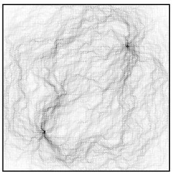
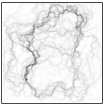
Figure 3. The current flow realizing (through Thomson’s Principle) the effective resistance between two points in the network associated with a sample of the GFF in a square of side $N:=100$ and $\gamma=0.2\gamma_{\text{\rm c}}$ (left) and $\gamma=0.5\gamma_{\text{\rm c}}$ (right). The source/sink of the current lie on the diagonal of the square (marked by the dark spots in the left figure). The intensity of the shade increases with the value of the current.

Our RSW proof is hugely inspired by [54], with the novelty of incorporating the (resistance) metric rather than merely considering connectivity. We remark that in a recent work [26], a RSW result was established for the Liouville FPP metric, again inspired by [54]. It is fair to say that the RSW result in the present paper is less complicated than that in [26], for the reason that we have the approximate duality in our context which was not available in [26]. However, our RSW proof has its own subtlety since, for instance, we need to consider crossings by whole collections of paths simultaneously. The RSW proof is carried out in Section 4. Once the effective resistances are under control, we move on to the proof of the results on random walks. The upper bound on the return probability is proved in Section 5.1 using the methods drawn from [37]. The lower bound on the return probability is more subtle as it requires showing that the effective resistance from $0$ to $v$ in $B(N)$ is bounded by the sum of the resistances from $0$ to $\partial B(N)$ and from $v$ to $\partial B(N$). This amounts to bounding a difference of effective resistances, which is not immediate from the estimates obtained thus far.

We approach this by invoking a concentric decomposition of the GFF along a sequence of annuli, which permits representing of the typical value of the resistance as an exponential of a random walk. The Law of the Iterated Logarithm then shows that the natural fluctuations of the effective resistance (which are of order $\mathrm{e}^{O(\sqrt{\log N})}$) can be beaten in at least one of the annuli. These key steps are the content of Proposition 5.8 and Lemma 5.9. As an immediate consequence, we then get recurrence and, in fact, also the bounds in Theorem 1.4.

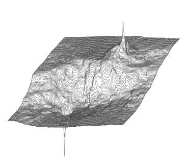
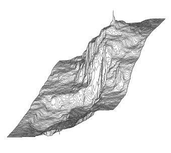
Figure 4. Voltage profiles for the same geometric setting as in Fig. 4 but for two different samples of GFF at $\gamma=0.3\gamma_{\text{\rm c}}$. Notice that the profile represents the probability that a random walk hits the highest point before hitting the lowest point in this profile. The plots indicate presence of macroscopic “barriers” where this probability undergoes a dramatic change.

1.3. Discussions and future directions

We feel that our method of estimating effective resistances provides a novel framework which may have applications in other planar random media. In fact, from our proofs we should be able to see that our method can be adapted to some other log-correlated Gaussian fields such as those considered in [43]. We refrain ourselves from doing so, for the reason that we do not yet know how to characterize the class of log-correlated Gaussian fields with subpolynomial (i.e., $N^{o(1)}$-like) growth of the effective resistances.

One important, and perhaps less conspicuous, ingredient of our proofs is the estimate of the effective resistance by means of the Gaussian concentration inequality. When the underlying random media is not a function of a Gaussian process, a derivation of such a concentration inequality seems to be a challenge. A natural class of non-Gaussian models where one should try to prove an analogue of Theorem 1.4 is that of gradient fields with uniformly convex interactions. Indeed, there the required concentration is implied by the Brascamp-Lieb inequality.

Concerning our future goals for the problem at hand, our first attempt will aim at the computation of the spectral dimension (which amounts to an almost sure version of (1.3)) and an upper bound on the diffusive exponent matching the lower bound in Theorem 1.3. Our ultimate goal is to prove existence of an appropriate scaling limit of the whole problem. This applies not only to the walk itself, but also to the resistance metric as well as the associated current and voltage configurations; see Fig. 3 and 4 for illustrations and the recent review [10, Chapter 16] for more specific questions.

1.4. Acknowledgements

The work of M.B. has been partially supported by NSF grants DMS-1407558 and DMS-1712632 and GAČR project P201/16-15238S. The work of J.D. and S.G. has been partially supported by NSF grant DMS-1455049 and Alfred Sloan fellowship. The authors wish to thank Takashi Kumagai, Hubert Lacoin, Rémi Rhodes, Steve Lalley, Vincent Vargas and Ofer Zeitouni for helpful discussions. We are also grateful to two anonymous referees for their numerous valuable suggestions that improved greatly the presentation of this work. The first draft of the paper was completed when both JD and SG were at the University of Chicago.

2. Generalized parallel and series laws

As noted above, our asymptotic statements on the random walk hinge on estimates of effective resistance between various sets in $\mathbb{Z}^{2}$. These will in turn rely crucially on a certain duality between the effective resistance and the effective conductance which will itself be based on the distributional equality of $\eta$ with $-\eta$. The exposition of our proofs thus starts with general versions of these duality statements. The results in this section hold for general networks; planarity is not required. They can be viewed as refinements of [42, Proposition 9.4] and are therefore of general interest as well.

2.1. Variational characterization of effective resistance

Let $\mathfrak{G}$ be a finite, unoriented, connected graph where each edge $e$ is equipped with a resistance $r_{e}\in{\mathbb{R}}_{+}$, where ${\mathbb{R}}_{+}$ denotes the set of positive reals. We will use $\mathfrak{G}$ to denote both the corresponding network as well as the underlying graph. Let $V(\mathfrak{G})$ and $E(\mathfrak{G})$ respectively denote the set of vertices and edges of $\mathfrak{G}$. We assume for simplicity that $\mathfrak{G}$ has no self-loops although we allow distinct vertices to be connected by multiple edges. For the purpose of counting we identify the two orientations of each edge; $E(\mathfrak{G})$ thus includes both orientations as one edge.

Two edges $e$ and $e^{\prime}$ of $\mathfrak{G}$ are said to be adjacent to each other, denoted as $e\sim e^{\prime}$, if they share at least one endpoint. Similarly a vertex $v$ and an edge $e$ are adjacent, denoted as $v\sim e$, if $v$ is an endpoint of the edge $e$. A path $P$ is a sequence of edges of $\mathfrak{G}$ such that any two successive edges are adjacent. We say that a path is edge self-avoiding if every edge appears in $P$ at most once. We also use $P$ to denote the subgraph of $\mathfrak{G}$ induced by the edge set of $P$.

For $u,v\in V(\mathfrak{G})$, a flow $\theta$ from $u$ to $v$ is an assignment of a number $\theta(x,y)$ to each oriented edge $(x,y)$ such that $\theta(x,y)=-\theta(y,x)$ and $\sum_{y\colon y\sim x}\theta(x,y)=0$ whenever $x\neq u,v$. The value of the flow $\theta$ is then the number $\text{val}(\theta):=\sum_{y\colon y\sim u}\theta(u,y)$; a unit flow then has this value equal to one. With these notions in place, the effective resistance $R_{\mathfrak{G}}(u,v)$ between $u$ and $v$ is defined by

$$R_{\mathfrak{G}}(u,v):=\inf_{\theta}\,\,\sum_{e\in E(\mathfrak{G})}r_{e}\,\theta_{\mathrm{e}}^{2}\,,$$ (2.1)

where the infimum (which is achieved because $\mathfrak{G}$ is finite) is over all unit flows from $u$ to $v$. Note that we sum over each edge $e\in E(\mathfrak{G})$ only once, taking advantage of the fact that $\theta_{e}$ appears in a square in this, and later expressions.

Recall that a multiset of elements of $A$ is a set of pairs $\{(a,i)\colon i=1,\dots,n_{a}\}$ for some $n_{a}\in\{0,1,\dots\}$ for each $a\in A$. We have the following alternative characterization of $R_{\mathfrak{G}}(u,v)$:

Proposition 2.1.

Let $\mathfrak{P}_{u,v}$ denote the set of all multisets of edge self-avoiding paths from $u$ to $v$. Then

$$R_{\mathfrak{G}}(u,v)=\inf_{\mathcal{P}\in\mathfrak{P}_{u,v}}\,\,\inf_{\{r_{e,P}\colon e\in E(\mathfrak{G}),\,P\in\mathcal{P}\}\in\mathfrak{R}_{\mathcal{P}}}\Bigl{(}\,\sum_{P\in\mathcal{P}}\frac{1}{\sum_{e\in P}r_{e,P}}\Bigr{)}^{-1}\,,$$ (2.2)

where $\mathfrak{R}_{\mathcal{P}}$ is the set of all assignments $\{r_{e,P}:e\in E(\mathfrak{G}),P\in\mathcal{P}\}\in\mathbb{R}_{+}^{E(\mathfrak{G})\times\mathcal{P}}$ such that

$$\sum_{P\in\mathcal{P}}\frac{1}{r_{e,P}}\leq\frac{1}{r_{e}}\,\text{\rm\ for all }\,e\in E(\mathcal{G})\,.$$ (2.3)

The infima in (2.2) are (jointly) achieved.

Proof. Let $R^{\star}$ denote the right hand side of (2.2). We will first prove $R_{\mathfrak{G}}(u,v)\leq R^{\star}$. Let thus $\mathcal{P}\in\mathfrak{P}_{u,v}$ and $\{r_{e,P}\colon e\in E,P\in\mathcal{P}\}\in\mathfrak{R}_{\mathcal{P}}$ subject to (2.3) be given. We will view each edge $e$ in $\mathfrak{G}$ as a parallel of a collection of edges $\{e_{P}\colon P\in\mathcal{P}\}$ where the resistance on $e_{P}$ is $r_{e,P}$ and, if the inequality in (2.3) for edge $e$ is strict, introduce a dummy edge $\tilde{e}$ with resistance $r_{\tilde{e}}$ such that $1/r_{\tilde{e}}=1/r_{e}-\sum_{P\in\mathcal{P}}1/r_{e,P}$. In this new network, $\mathcal{P}$ can be identified with a collection of disjoint paths where (by the series law) each path $P\in\mathcal{P}$ has total resistance $\sum_{e\in P}r_{e,P}$. The parallel law guarantees

$$R_{\mathfrak{G}}(u,v)\leq\Bigl{(}\,\sum_{P\in\mathcal{P}}\frac{1}{\sum_{e\in P}r_{e,P}}\Bigr{)}^{-1}$$ (2.4)

which proves $R_{\mathfrak{G}}(u,v)\leq R^{\star}$ as desired.

Next, we turn to proving that $R_{\mathfrak{G}}(u,v)\geq R^{\star}$ and that the infima in (2.2) are achieved.

Let $\theta^{\star}$ be the unit flow achieving the infimum in (2.1). We will run an algorithm that inductively identifies a sequence of flows $\theta_{k}$ (not necessarily of unit value) and paths $P_{k}$ from $u$ and $v$. A key fact to note is that, if $e\mapsto\theta(e)$ is a flow from $u$ to $v$ with $\text{val}(i)>0$, then there is an edge self-avoiding path $P$ from $u$ to $v$ such that $\theta(e)>0$ for each $e\in P$ oriented in the direction of $P$. This follows by the fact that, at all vertices except the source and the sink, having an edge with a positive incoming flow forces an edge with a positive outgoing flow.

The algorithm runs as follows. INITIATE by setting $\theta_{0}:=\theta^{\star}$. If $\text{val}(\theta_{k-1})=0$ then STOP, else use the above observation to find a simple path $P_{k}$ from $u$ to $v$ where $\theta_{k-1}(e)>0$ for each edge $e\in P_{k}$ oriented in the direction of the path. Then set $\alpha_{k}:=\min_{e\in P_{k}}|\theta_{k-1}(e)|$, let

$$\theta_{k}(e):=\theta_{k-1}(e)-\alpha_{k}\,\text{sign}(\theta_{k-1}(e))1_{\{e\in P_{k}\}}$$ (2.5)

and, noting that $\theta_{k}$ is a flow from $u$ to $v$ with $\text{val}(\theta)\geq 0$, REPEAT.

As $\{e\in E(\mathfrak{G})\colon\theta_{k}(e)\neq 0\}$ is strictly decreasing in $k$, the algorithm will terminate after a finite number of steps. Also $k\mapsto|\theta_{k}(e)|$ and $k\mapsto\text{val}(\theta_{k})$ are decreasing, and so

$$\forall e\in E(\mathfrak{G})\colon\,\,\,\sum_{k\colon e\in P_{k}}\alpha_{k}\leq|\theta^{\star}(e)|\qquad\text{and}\qquad\sum_{k}\alpha_{k}=\text{\rm val}(\theta^{\star})=1.$$ (2.6)

Set $r_{e,P_{k}}:=|\theta^{\star}(e)|r_{e}/\alpha_{k}$ and compute

$$R_{\mathrm{eff}}(u,v) =\sum_{e\in E(\mathfrak{G})}r_{e}\,\theta^{\star}(e)^{2}\geq\sum_{e\in E(\mathfrak{G})}\,r_{e}|\theta^{\star}(e)|\sum_{k\colon e\in P_{k}}\alpha_{k}$$ (2.7)

$$=\sum_{e\in E(\mathfrak{G})}\,\sum_{k\colon e\in P_{k}}r_{e,P_{k}}\alpha_{k}^{2}=\sum_{k}\,\alpha_{k}^{2}\Bigl{(}\sum_{e\in P_{k}}r_{e,P_{k}}\Bigr{)}.$$

Denoting the quantity in the large parentheses by $R_{k}$, of all positive $\alpha_{k}$’s subject to the equality in (2.6), the right-hand side is minimized by $\alpha_{k}:=\frac{1/R_{k}}{\sum_{j}1/R_{j}}$. As (2.6) shows $\sum_{k}1/r_{e,P_{k}}\leq 1/r_{e}$ for each $e\in E(\mathfrak{G})$, the claim follows. ∎

A slightly augmented version of the above proof in fact yields:

Proposition 2.2.

Let $\mathfrak{T}_{u,v}$ be the set of all multisets of edges of $\mathfrak{G}$ that, if considered as a graph on $V(\mathfrak{G})$, contain a path between $u$ and $v$. Then

$$R_{\mathfrak{G}}(u,v)=\inf_{\mathcal{T}\in\mathfrak{T}_{u,v}}\inf_{\{r_{e,T}:e\in E(\mathfrak{G}),T\in\mathcal{T}\}\in\mathfrak{R}_{\mathcal{T}}}\Bigl{(}\,\sum_{T\in\mathcal{T}}\frac{1}{\sum_{e\in T}r_{e,T}}\Bigr{)}^{-1}\,,$$ (2.8)

where $\mathfrak{R}_{\mathcal{T}}$ is the set of all assignments $\{r_{e,T}\colon e\in E(\mathfrak{G}),T\in\mathcal{T}\}\in\mathbb{R}_{+}^{E(\mathfrak{G})\times\mathcal{T}}$ such that

$$\sum_{T\in\mathcal{T}}\frac{1}{r_{e,T}}\leq\frac{1}{r_{e}}\,\text{\rm\ for all }\,e\in E(\mathcal{G})\,.$$ (2.9)

The infima are jointly achieved for $\mathcal{T}$ being a subset of $\mathfrak{P}_{u,v}$.

Proof. Let $R^{\star}$ denote the right-hand side of (2.8). Obviously, $\mathfrak{P}_{u,v}\subseteq\mathfrak{T}_{u,v}$ so restricting the first infimum to $\mathcal{T}\in\mathfrak{P}_{u,v}$, Proposition 2.1 shows $R_{\mathfrak{G}}(u,v)\geq R^{\star}$. (This will also ultimately give that the minimum is achieved over collections of paths.) To get $R_{\mathfrak{G}}(u,v)\leq R^{\star}$, let us consider an assignment $\{r_{e,T}\colon e\in E(\mathfrak{G}),T\in\mathcal{T}\}$ satisfying (2.9). For each $T\in\mathcal{T}$, let $P_{T}$ denote an arbitrarily chosen edge self-avoiding path between $u$ and $v$ formed by edges in $T$. Then, defining $r_{e,P_{T}}:=r_{e,T}$ for each $T\in\mathcal{T}$, we find that the assignment $\{r_{e,P_{T}}\colon e\in E(\mathfrak{G}),T\in\mathcal{T}\}$ satisfies (2.3). Now the claim follows from the simple observation that $\sum_{e\in P_{T}}r_{e,p_{T}}\leq\sum_{e\in P_{T}}r_{e,T}$. ∎

2.2. Variational characterization of effective conductance

An alternative way to approach an electric network is using conductances. We write $c_{e}:=1/r_{e}$ for the edge conductance on $e$, and define the effective conductance between $u$ and $v$ by

$$C_{\mathfrak{G}}(u,v):=\inf_{F}\,\sum_{e\in E(\mathfrak{G})}c_{e}\,\bigl{[}F(e_{+})-F(e_{-})\bigr{]}^{2}\,,$$ (2.10)

where $e_{\pm}$ are the two endpoints of the edge $e$ (in some a priori orientation) and the infimum is over all functions $F\colon V\to\mathbb{R}$ satisfying $F(u)=1$ and $F(v)=0$. The infimum is again achieved by the fact that $\mathfrak{G}$ is finite. The fundamental electrostatic duality is then expressed as

$$C_{\mathfrak{G}}(u,v)=\frac{1}{R_{\mathfrak{G}}(u,v)}$$ (2.11)

and our aim is to capitalize on this relation further by exploiting the geometric duality between paths and cutsets. Here we say that a set of edges $\pi$ is a cutset between $u$ and $v$ (or that $\pi$ separates $u$ from $v$) if each path from $u$ to $v$ uses an edge in $\pi$.

Proposition 2.3.

Let $\varPi_{u,v}$ denote the set of all finite collections of cutsets between $u$ and $v$. Then

$$C_{\mathfrak{G}}(u,v)=\inf_{\Pi\in{\varPi}_{u,v}}\inf_{\{c_{e,\pi}\colon e\in E(\mathfrak{G}),\pi\in\Pi\}\in\mathfrak{C}_{\Pi}}\Bigl{(}\,\sum_{\pi\in\Pi}\frac{1}{\sum_{e\in\pi}c_{e,\pi}}\Bigr{)}^{-1}\,,$$ (2.12)

where $\mathfrak{C}_{\Pi}$ is the set of all assignments $\{c_{e,\pi}\colon e\in E(\mathfrak{G}),\pi\in\Pi\}\in\mathbb{R}_{+}^{E(\mathfrak{G})\times\Pi}$ such that

$$\sum_{\pi\in\Pi}\frac{1}{c_{e,\pi}}\leq\frac{1}{c_{e}}\,\text{\rm\ for all }\,e\in E(\mathfrak{G})\,.$$ (2.13)

The infima in (2.12) are (jointly) achieved.

Proof. The proof is structurally similar to that of Proposition 2.1. Denote by $C^{\star}$ the quantity on the right hand side of (2.12). We will first prove $C_{\mathfrak{G}}(u,v)\leq C^{\star}$. Pick $\Pi\in\varPi$ and $\{c_{e,\pi}\colon e\in E(\mathfrak{G}),\pi\in\Pi\}\in\mathfrak{C}_{\Pi}$ subject to (2.13). Now view each edge $e$ as a series of a collection of edges $\{e_{\pi}:e\in\pi,\pi\in\Pi\}$ where the conductance on $e_{\pi}$ is $c_{e,\pi}$ and, if the inequality in (2.13) is strict, introduce a dummy edge $\tilde{e}$ with conductance $c_{\tilde{e}}$ such that $1/c_{\tilde{e}}=1/c_{e}-\sum_{\pi\in\Pi}1/c_{e,\pi}$. In this new network, $\Pi$ can be identified with a collection of disjoint cutsets, where the cutset $\pi\in\Pi$ has total conductance $\sum_{e\in\pi}c_{e,\pi}$. The Nash-Williams Criterion then shows

$$C_{\mathfrak{G}}(u,v)\leq\Bigl{(}\,\sum_{\pi\in\Pi}\frac{1}{\sum_{e\in\pi}c_{e,\pi}}\Bigr{)}^{-1}$$ (2.14)

thus proving $C_{\mathfrak{G}}(u,v)\leq C^{\star}$ as desired.

Next, we turn to proving $C_{\mathfrak{G}}(u,v)\geq C^{\star}$ and that the infima in (2.12) are attained. Let $F^{\star}$ be a function that achieves the infimum in (2.10). This function is discrete harmonic in the sense that $\mathcal{L}F^{\star}(x)=0$ for $x\neq u,v$, where

$$\mathcal{L}f(x):=\sum_{y\colon y\sim x}c_{(x,y)}\,\bigl{[}f(y)-f(x)\bigr{]}.$$ (2.15)

This is an important property in light of the following observation: If $f\colon V(\mathfrak{G})\to{\mathbb{R}}$ is such that $f(u)>f(v)$ and $\mathcal{L}f(x)=0$ for $x\not\in D\cup\{v\}$ where

$$D:=\bigl{\{}x\in V(\mathfrak{G})\colon f(x)=f(u)\bigr{\}},$$ (2.16)

then $\pi:=\{(x,y)\in E(\mathfrak{G})\colon x\in D,y\not\in D\}$ defines a cut-set $\pi$ from $u$ to $v$ such that $f(x)>f(y)$ holds for each edge $(x,y)\in\pi$ oriented so that $x\in D$ and $y\not\in D$.

We will now define a sequence of functions $F_{k}\colon V(\mathfrak{G})\to{\mathbb{R}}$ and cuts $\pi_{k}$ by the following algorithm: INITIATE by $F_{0}:=f^{\star}$. If $F_{k-1}$ is constant then STOP, else use the above observation with $D_{k-1}$ related to $F_{k-1}$ as $D$ is to $F$ in (2.16) to define $\pi_{k}:=\{(x,y)\in E(\mathfrak{G})\colon x\in D_{k},y\not\in D_{k}\}$. Noting that $F_{k-1}(x)>F_{k-1}(y)$ for each edge $(x,y)\in\pi$ (oriented to point from $u$ to $v$), set $\alpha_{k}:=\min_{(x,y)\in\pi}|F_{k-1}(x)-F_{k-1}(y)|$ and let

$$F_{k}(z):=F_{k-1}(z)-\alpha_{k}\,1_{D_{k-1}}(z).$$ (2.17)

Then REPEAT.

As is checked by induction, $k\mapsto D_{k}$ is strictly increasing while $k\mapsto F_{k}$ is non-increasing with $F_{k}=F^{\star}$ on $V(\mathfrak{G})\smallsetminus D_{k}$. In particular, we have $\mathcal{L}F_{k}(x)=0$ for all $x\not\in D_{k}\cup\{v\}$ and so the above observation can repeatedly be used. The premise of the strict inequality $F_{k}(u)>F_{k}(v)$ for all but the final step is the consequence of the Maximum Principle.

Now we perform some elementary calculations. Let $\Pi$ denote the set of the cutsets $\pi_{k}$ identified above. For each edge $(x,y)$ and each $\pi_{k}\in\Pi$, define

$$c_{e,\pi_{k}}:=\frac{|F^{\star}(y)-F^{\star}(x)|}{\alpha_{k}}\,c_{e}.$$ (2.18)

The construction and the fact that $F^{\star}(u)=1$ and $F^{\star}(v)=0$ imply

$$\sum_{k}\alpha_{k}=1\,.$$ (2.19)

For any $e=(x,y)$, we also get

$$\sum_{k\colon e\in\pi_{k}}\alpha_{k}=\bigl{|}F^{\star}(y)-F^{\star}(x)\bigr{|}.$$ (2.20)

In particular, the collection $\{c_{e,\pi}\colon\pi\in\Pi,\,e\in\pi\}$ obeys (2.13). Moreover, (2.18) then shows, for any $e=(x,y)$,

$$\sum_{k\colon e\in\pi_{k}}c_{e,\pi_{k}}\alpha_{k}^{2}=c_{e}\bigl{|}F^{\star}(y)-F^{\star}(x)\bigr{|}\sum_{k\colon e\in\pi_{k}}\alpha_{k}=c_{e}\bigl{|}F^{\star}(y)-F^{\star}(x)\bigr{|}^{2}.$$ (2.21)

Summing over $e\in E(\mathfrak{G})$ and rearranging the sums yields

$$C_{\mathfrak{G}}(u,v)=\sum_{e\in E(\mathfrak{G})}\,\,\sum_{k\colon e\in\pi_{k}}c_{e,\pi_{k}}\alpha_{k}^{2}=\sum_{k}\alpha_{k}^{2}\Bigl{(}\sum_{e\colon e\in\pi_{k}}c_{e,\pi_{k}}\Bigr{)}\,.$$ (2.22)

Denoting the sum in the large parentheses by $C_{k}$, among all non-negative $\alpha_{k}$’s satisfying (2.19), the right-hand side is minimal for $\alpha_{k}:=\frac{1/C_{k}}{\sum_{j}1/C_{j}}$. This shows “$\geq$” in (2.12). ∎

Propositions 2.1 and 2.3 seem to be closely related to various variational characterizations of effective resistance/conductance by way of optimizing over random paths and cutsets. These are rooted in the Nash-Williams criterion and Terry Lyons’ random-path method for bounding effective resistance (which can be shown to be sharp). The ultimate statements of these characterizations can be found in Berman and Konsowa [8].

2.3. Restricted notion of effective resistance

Propositions 2.1 and 2.3 naturally lead to restricted notions of resistance and conductance obtained by limiting the optimization to only subsets of paths and cutsets, respectively. For the purpose of the current paper we will only be concerned with effective resistance. To this end, for each collection $\mathcal{A}$ of finite sets of elements from $E(\mathfrak{G}$), we define

$$R_{\mathfrak{G}}(\mathcal{A}):=\inf_{\{r_{e,A}:e\in E(\mathcal{A}),\,A\in\mathcal{A}\}\in\mathfrak{R}_{\mathcal{A}}}\Bigl{(}\,\sum_{A\in\mathcal{A}}\frac{1}{\sum_{e\in A}r_{e,A}}\Bigr{)}^{-1}\,,$$ (2.23)

where $E(\mathcal{A}):=\bigcup_{A\in\mathcal{A}}A$ and where $\mathfrak{R}_{\mathcal{A}}$ is the set of all $\{r_{e,A}:e\in E(\mathcal{A}),\,A\in\mathcal{A}\}\in\mathbb{R}_{+}^{E(\mathcal{A})\times\mathcal{A}}$ such that

$$\sum_{A\in\mathcal{A}}\frac{1}{r_{e,A}}\leq\frac{1}{r_{e}}\,\text{\rm\ for all }\,e\in E(\mathcal{A})\,.$$ (2.24)

We refer to $R_{\mathfrak{G}}(\mathcal{A})$ as the effective resistance restricted to $\mathcal{A}$. By taking suitable $r_{e,P}$, the map $\mathcal{A}\mapsto R_{\mathfrak{G}}(\mathcal{A})$ is shown to be non-increasing with respect to the set inclusion. We will mostly be interested in $R_{\mathfrak{G}}(\mathcal{A})$ when $\mathcal{A}$ is a set of edge self-avoiding paths from $u$ to $v$. In particular, $R_{\mathfrak{G}}(\mathcal{A})=R_{\mathfrak{G}}(u,v)$ when $\mathcal{A}$ is the set of all the edge self-avoiding paths between $u$ and $v$. The following result is a generalization of the triangle inequality for the effective resistance.

Lemma 2.4.

Let $\mathcal{P}_{1},\mathcal{P}_{2},\cdots,\mathcal{P}_{k}$ be collections of paths such that for any choice of $P_{i}$ from $\mathcal{P}_{i}$ for each $1\leq i\leq k$, the graph union $\bigcup_{1\leq i\leq k}P_{i}$ contains a path between $u$ and $v$. Then

$$R_{\mathfrak{G}}(u,v)\leq\sum_{i=1}^{k}R_{\mathfrak{G}}(\mathcal{P}_{i})\,.$$ (2.25)

Proof. Define the edge sets $E_{1},E_{2},\cdots,E_{k}$ recursively by setting $E_{1}:=\bigcup_{P\in\mathcal{P}_{1}}E(P)$ and letting $E_{j}:=\bigcup_{P\in\mathcal{P}_{j}}E(P)\setminus\bigcup_{i<j}E_{i}$ for $k\geq j>1$. Let $\{r_{e,P}\colon e\in E(\mathfrak{G}),P\in\mathcal{P}_{i}\}$ be a vector in ${\mathbb{R}}_{+}^{E(\mathfrak{G})\times\mathcal{P}_{i}}$ satisfying (2.24) for all $i$. For each $i=1,\dots,k$ and each $P\in\mathcal{P}_{i}$, define $\rho_{i,P}$ by

$$\rho_{i,P}:=\frac{\Bigl{(}\,\sum_{e\in E(P)}r_{e,P}\bigr{)}^{-1}}{\sum_{P\in\mathcal{P}_{i}}\Bigl{(}\,\sum_{e\in E(P)}r_{e,P}\bigr{)}^{-1}}\,.$$ (2.26)

Also for $e\in E_{i}$ and $P_{1},P_{2},\cdots,P_{k}\,$ in $\mathcal{P}_{1},\mathcal{P}_{2},\cdots,\mathcal{P}_{k}$ respectively, define

$$r_{e;P_{1},P_{2},\cdots,P_{k}}:=r_{e,P_{i}}\prod_{j\neq i}\frac{1}{\rho_{j,P_{j}}}\,.$$ (2.27)

Notice that for any $e\in E_{i}$,

$$\sum_{\begin{subarray}{c}P_{j}\in\mathcal{P}_{j},\\ 1\leq j\leq k\end{subarray}}\frac{1}{r_{e;P_{1},P_{2},\cdots,P_{k}}}=\sum_{P_{i}\in\mathcal{P}_{i}}\frac{1}{r_{e,P_{i}}}\leq\frac{1}{r_{e}}\,,$$ (2.28)

where the first equality follows from the fact that $\sum_{P\in\mathcal{P}_{j}}\rho_{j,P}=1$ for all $j$ and the last inequality is a consequence of (2.24).

The above definitions also immediately give

$$\sum\limits_{e\in\bigcup_{1\leq i\leq k}E(P_{j})}r_{e;P_{1},P_{2},\cdots,P_{k}} \leq\sum\limits_{1\leq i\leq k}\sum\limits_{e\in E(P_{i})}\frac{r_{e,P_{i}}}{\prod_{j\neq i}\rho_{j,P_{j}}}$$ (2.29)

$$=\sum\limits_{1\leq i\leq k}\frac{\big{(}\sum_{P\in\mathcal{P}_{i}}\frac{1}{\sum_{e\in E(P)}r_{e,P}}\big{)}^{-1}}{\prod_{1\leq j\leq k}\rho_{j,P_{j}}}$$

As (2.28) holds, Proposition 2.2 with $T$ being the set of edges in $P_{1},\dots,P_{k}$ yields

$$R_{\mathfrak{G}}(u,v) \leq\Biggl{(}\,\sum_{\begin{subarray}{c}P_{j}\in\mathcal{P}_{j},\\ 1\leq j\leq k\end{subarray}}\frac{1}{\sum\limits_{e\in\bigcup_{1\leq i\leq k}E(P_{j})}r_{e;P_{1},P_{2},\cdots,P_{k}}}\Biggr{)}^{-1}$$ (2.30)

$$\leq\Biggl{(}\biggl{[}\,\sum\limits_{1\leq i\leq k}\Bigl{(}\sum_{P\in\mathcal{P}_{i}}\frac{1}{\sum_{e\in E(P)}r_{e,P}}\Bigr{)}^{-1}\biggr{]}^{-1}\sum_{\begin{subarray}{c}P_{j}\in\mathcal{P}_{j},\\ 1\leq j\leq k\end{subarray}}\prod_{1\leq j\leq k}\rho_{j,P_{j}}\Biggr{)}^{-1}$$

$$=\sum\limits_{1\leq i\leq k}\Bigl{(}\,\sum_{P\in\mathcal{P}_{i}}\frac{1}{\sum_{e\in E(P)}r_{e,P}}\Bigr{)}^{-1}\,,$$

where we again used $\sum_{P\in\mathcal{P}_{j}}\rho_{j,P}=1$ in the last step. Since (2.30) holds for all choices of $\{r_{e,P}\colon e\in E(\mathfrak{G}),P\in\mathcal{P}_{i}\}$ satisfying (2.24), the claim follows from (2.23). ∎

A similar upper bound holds also for the effective conductance.

Lemma 2.5.

Let $\mathcal{P}_{1},\dots,\mathcal{P}_{k}\in\mathfrak{P}_{u,v}$ be such that every path from $u$ to $v$ lies in the union $\bigcup_{1\leq i\leq k}\mathcal{P}_{i}$. Then

$$C_{\mathfrak{G}}(u,v)\leq\sum_{1\leq i\leq k}R_{\mathfrak{G}}(\mathcal{P}_{i})^{-1}\,.$$ (2.31)

Proof. This is a direct consequence of Proposition 2.1. Indeed, write $R_{\mathfrak{G}}(u,v)^{-1}$ as the suprema of $\sum_{P\in\mathcal{P}}(\sum_{e\in P}r_{e,P})^{-1}$ over $\mathcal{P}$ and $r_{e,P}$ satisfying (2.3). Next bound the sum over $P$ by the sum over $i=1,\dots,k$ and the sum over $P\in\mathcal{P}\cap\mathcal{P}_{i}$ and observe, since $\sum_{P\in\mathcal{P}\cap\mathcal{P}_{i}}1/r_{e,P}\leq\sum_{P\in\mathcal{P}}1/{r_{e,P}}\leq 1/r_{e}$, we have

$$\sum_{i=1}^{k}\sum_{P\in\mathcal{P}\cap P_{i}}\frac{1}{\sum_{e\in P}r_{e,P}}\leq\sum_{i=1}^{k}R_{\mathfrak{G}}(\mathcal{P}_{i})^{-1}.$$ (2.32)

As this holds for all $\mathcal{P}$ and all admissible $r_{e,P}$, the claim follows from (2.11).∎

We note (and this will be useful later) that, in standard treatments of electrostatic theory on graphs, the notions of effective resistance/conductance are naturally defined between subsets (as opposed to just single vertices) of the underlying network. A simplest way to reduce this to our earlier definitions is by “ shorting” the vertices in these sets together. Explicitly, given two non-empty disjoint sets $A,B\subseteq V(\mathfrak{G})$ consider a network $\mathfrak{G}^{\prime}$ where all edges in $(A\times A)\cup(B\times B)$ have been removed and the vertices in $A$ identified as one vertex $\langle A\rangle$ — with all edges in $\mathfrak{G}$ with exactly one endpoint in $A$ now “pointing” to $\langle A\rangle$ in $\mathfrak{G}^{\prime}$ — and the vertices in $B$ similarly identified as one vertex $\langle B\rangle$. Then we define

$$R_{\mathfrak{G}}(A,B):=R_{\mathfrak{G}^{\prime}}\bigl{(}\langle A\rangle,\langle B\rangle\bigr{)}\quad\text{\rm and}\quad C_{\mathfrak{G}}(A,B):=C_{\mathfrak{G}^{\prime}}\bigl{(}\langle A\rangle,\langle B\rangle\bigr{)}.$$ (2.33)

Note that, for one-point sets, $R_{\mathfrak{G}}(\{u\},\{v\})$ coincides with $R_{\mathfrak{G}}(u,v)$, and similarly for the effective conductance. The electrostatic duality also holds, $R_{\mathfrak{G}}(A,B)=1/C_{\mathfrak{G}}(A,B)$.

2.4. Self-duality

The results in this section are consequences of Propositions 2.2 and 2.3. Observe that the similarity of the two formulas (2.8) (also (2.2)) and (2.12) naturally leads to the consideration of self-dual situations — i.e., those in which the resistances $r_{e}$ can somehow be exchanged for the conductances $c_{e}$ and the paths can be exchanged for the cutsets. An example of this is the network $\mathbb{Z}^{2}_{\eta}$ where the distributional identity $\eta\overset{\text{\rm law}}{=}-\eta$ (recall from the introduction that $\eta$ is a centered Gaussian field) makes the associated resistances $\{r_{e}\colon e\in E(\mathbb{Z}^{2})\}$ equidistributed to the conductances $\{c_{e}\colon e\in E(\mathbb{Z}^{2})\}$; planarity then associates cutsets with paths. To formalize this situation, given a network $\mathfrak{G}$ we define its reciprocal $\mathfrak{G}^{\star}$ as the network with the same underlying graph but with the resistances swapped for the conductances. An edge $e$ in network $\mathfrak{G}^{\star}$ thus has resistance $r_{e}^{\star}:=1/r_{e}$, where $r_{e}$ is the resistance of $e$ in network $\mathfrak{G}$.

Lemma 2.6.

Let $\mathfrak{D}$ denote the maximum vertex degree in $\mathfrak{G}$ and let $\rho_{\max}$ denote the maximum ratio of the resistances of any pair of adjacent edges in $\mathfrak{G}$. Given two pairs $(A,B)$ and $(C,D)$ of disjoint, nonempty subsets of $V(\mathfrak{G})$, suppose that every path between $A$ and $B$ shares a vertex with every path between $C$ and $D$. Then

$$R_{\mathfrak{G}}(A,B){R}_{\mathfrak{G}^{\star}}(C,D)\geq\frac{1}{4\mathfrak{D}^{2}\rho_{\max}}\,.$$ (2.34)

Proof. The proof is based on the fact that every path $P$ between $C$ and $D$ defines a cutset $\pi_{P}$ between $A$ and $B$ by taking $\pi_{P}$ to be the set of all edges adjacent to any edge in $P$, but not including the edges in $(A\times A)\cup(B\times B)$. By the electrostatic duality we just need to show

$$C_{\mathfrak{G}}(A,B)\leq 4\mathfrak{D}^{2}\rho_{\max}{R}_{\mathfrak{G}^{\star}}(C,D)\,.$$ (2.35)

To this end, given any $\mathcal{P}\in\mathfrak{P}_{C,D}$ (i.e., $\mathcal{P}$ is a multiset of edge self-avoiding paths between $C$ and $D$) let us pick positive numbers $\{r^{\prime}_{e,P}:e\in E(\mathcal{P}),P\in\mathcal{P}\}$ such that

$$\sum_{P\in\mathcal{P}}\frac{1}{r^{\prime}_{e,P}}\leq\frac{1}{c_{e}}\,\text{\rm\ for all }\,e\in E(\mathcal{P})\,.$$ (2.36)

For any edge $e$ and any path $P\in\mathcal{P}$, let $N_{P}(e)$, $N_{\mathcal{P}}(e)$ and $N(e)$ denote the sets of all edges in $E(P)$, $E(\mathcal{P})$ and $E(\mathfrak{G})$ that are adjacent to $e$, respectively. For any $e\in E(\mathcal{P})$ and any $P\in\mathcal{P}$, let $\theta_{e,P}:=c_{e}/r^{\prime}_{e,P}$ and note that $\theta_{e,P}$’s are positive numbers satisfying $\sum_{P\in\mathcal{P}}\theta_{e,P}\leq 1$ for all $e\in E(\mathcal{P})$. As a consequence, if we define

$$c_{e,\pi_{P}}:=\frac{c_{e}}{\sum\limits_{e^{\prime}\in N_{\mathcal{P}^{\prime}}(e)}\theta_{e^{\prime},P}}|N_{\mathcal{P}}(e)|$$ (2.37)

then $\{c_{e,\pi_{P}}\colon e\in\bigcup_{P\in\mathcal{P}}\pi_{P},\,P\in\mathcal{P}\}$ satisfies (2.13). Now fix a path $P$ in $\mathcal{P}$ and compute, invoking the definitions of $\mathfrak{D}$, $\rho_{\max}$ and also Jensen’s inequality in the second step:

$$\sum\limits_{e\in\pi_{P}}c_{e,\pi_{P}} =\sum\limits_{e\in\pi_{P}}\frac{c_{e}}{\sum\limits_{e^{\prime}\in N_{\mathcal{P}}(e)}\theta_{e^{\prime},P}}|N_{\mathcal{P}}(e)|\leq 2\mathfrak{D}\sum\limits_{e\in\pi_{P}}\frac{c_{e}}{\sum\limits_{e^{\prime}\in N_{P}(e)}\theta_{e^{\prime},P}}|N_{P}(e)|$$ (2.38)

$$\leq 2\mathfrak{D}\sum\limits_{e\in\pi_{P}}\Big{(}\frac{c_{e}}{|N_{P}(e)|}\sum_{e^{\prime}\in N_{P}(e)}\frac{1}{\theta_{e^{\prime},P}}\Big{)}\leq 2\mathfrak{D}\sum_{\begin{subarray}{c}e\in E(\mathfrak{G}),e^{\prime}\in P\\ e\sim e^{\prime}\end{subarray}}\frac{c_{e}}{\theta_{e^{\prime},P}}$$

$$=2\mathfrak{D}\sum\limits_{e^{\prime}\in P}\frac{\sum\limits_{e\in N(e^{\prime})}c_{e}}{\theta_{e^{\prime},P}}\leq 4\mathfrak{D}^{2}\rho_{\max}\sum\limits_{e^{\prime}\in P}\frac{c_{e^{\prime}}}{\theta_{e^{\prime},P}}=4\mathfrak{D}^{2}\rho_{\max}\sum\limits_{e^{\prime}\in P}r^{\prime}_{e^{\prime},P}\,.$$

Hence we get by Proposition 2.3

$$C_{\mathfrak{G}}(A,B)\leq\Bigl{(}\,\sum_{P\in\mathcal{P}^{\prime}}\frac{1}{\sum_{e\in\pi_{P}}c_{e,\pi_{P}}}\Bigr{)}^{-1}\leq 4{\mathfrak{D}}^{2}\rho_{\max}\Bigl{(}\,\sum_{P\in\mathcal{P}^{\prime}}\frac{1}{\sum_{e\in P}r^{\prime}_{e,P}}\Bigr{)}^{-1}\,.$$ (2.39)

As this holds for any choice of $\mathcal{P}$ and positive numbers $\{r^{\prime}_{e,P}:e\in E(\mathcal{P}),P\in\mathcal{P}\}$ satisfying (2.36), we get (2.35) as desired. ∎

A crucial fact underlying the proof of the previous lemma was that one could obtain a cut set for $\mathcal{P}$ from a path $P$ in $\mathcal{P}$ by taking union of all edges adjacent to vertices in $P$. In the same setup, we get a corresponding result also for effective conductances. Indeed, we have:

Lemma 2.7.

For the same setting and notation as in Lemma 2.6, assume that for every cutset $\pi$ between $C$ and $D$, the subgraph induced by the set of all edges that are adjacent to some edge in $\pi$ contains a path in $\mathfrak{P}_{A,B}$. Then

$$C_{\mathfrak{G}}(A,B){C}_{\mathfrak{G}^{\star}}(C,D)\geq\frac{1}{4{\mathfrak{D}}^{2}\rho_{\max}}\,.$$ (2.40)

Proof. For any cutset $\pi$ between $C$ and $D$, let $T_{\pi}$ denote the set of all edges that are adjacent to some edge in $\pi$. Thus $T_{\pi}$ contains a path in $\mathfrak{P}_{A,B}$ by the hypothesis of the lemma. Also recall from the statement of Proposition 2.3 that $\varPi(C,D)$ is the set of all finite collections of cutsets between $C$ and $D$. Now given any $\Pi\in\varPi_{C,D}$, we pick a collection of positive numbers $\{c_{e,\pi}^{\star}\colon e\in\bigcup_{\pi\in\Pi}T_{\pi},\pi\in\Pi\}$ such that

$$\sum_{\pi\in\Pi}\frac{1}{c_{e,\pi}^{\star}}\leq\frac{1}{r_{e}}\,.$$ (2.41)

Following the exact same sequence of steps as in the proof of Lemma 2.6, we now find $\{r_{e,T_{\pi}}\colon e\in\pi,\pi\in\Pi\}$ satisfying (2.9) such that

$$\Bigl{(}\,\sum_{\pi\in\Pi}\frac{1}{\sum_{e\in T_{\pi}}r_{e,T_{\pi}}}\Bigr{)}^{-1}\leq 4{\mathfrak{D}}^{2}\rho_{\max}\Bigl{(}\,\sum_{\pi\in\Pi}\frac{1}{\sum_{e\in\pi}c_{e,\pi}^{\star}}\Bigr{)}^{-1}\,.$$ (2.42)

Proposition 2.2 then implies

$$R_{\mathfrak{G}}(A,B)\leq\Bigl{(}\,\sum_{\pi\in\Pi}\frac{1}{\sum_{e\in T_{\pi}}r_{e,T_{\pi}}}\Bigr{)}^{-1}\leq 4{\mathfrak{D}}^{2}\rho_{\max}\Bigl{(}\,\sum_{\pi\in\Pi}\frac{1}{\sum_{e\in\pi}c_{e,\pi}^{\star}}\Bigr{)}^{-1}\,.$$ (2.43)

As this holds for all choices of $\Pi$ and $\{c_{e,\pi}^{\star}\colon e\in\pi,\pi\in\Pi\}$ satisfying (2.41), we get the desired inequality (2.40). ∎

3. Preliminaries on Gaussian processes

Before we move on to the main line of the proof, we need to develop some preliminary control on the underlying Gaussian fields. The goal of this section is to amass the relevant technical claims concerning Gaussian processes and, in particular, the GFF. An impatient, or otherwise uninterested, reader may consider only skimming through this section and returning to it when the relevant claims are used in later proofs.

3.1. Some standard inequalities

We start by recalling, without proof, a few standard facts about general Gaussian processes:

Lemma 3.1 (Theorem 7.1 in [39]).

Given a finite set $A$, consider a centered Gaussian process $\{X_{v}:v\in A\}$. Then, for $x>0$,

$$\mathbb{P}\biggl{(}\,\Bigl{|}\max_{v\in A}X_{v}-\mathbb{E}\max_{v\in A}X_{v}\Bigr{|}\geq x\biggr{)}\leq 2\mathrm{e}^{-x^{2}/2\sigma^{2}}\,,$$ (3.1)

where $\sigma^{2}:=\max_{v\in A}\mathbb{E}(X_{v}^{2})$.

Lemma 3.2 (Theorem 4.1 in [1]).

Suppose $(S,d)$ is a finite metric space such that $\max_{s,t\in S}d(s,t)=1$ and assume there are $\beta,K_{1}\in(0,\infty)$ such that for every $\epsilon\in(0,1]$, the $\epsilon$-covering number $N_{\epsilon}(S,d)$ of $(S,d)$ obeys $N_{\epsilon}(S,d)\leq K_{1}\epsilon^{-\beta}$. Then for any $\alpha,K_{2}\in(0,\infty)$ and any centered Gaussian process $\{X_{s}\}_{s\in S}$ satisfying

$$\sqrt{\mathbb{E}(X_{s}-X_{s^{\prime}})^{2}}\leq K_{2}\,d(s,s^{\prime})^{\alpha},\qquad s,s^{\prime}\in S,$$ (3.2)

we have

$$\mathbb{E}\bigl{(}\,\max_{s\in A}|X_{s}|\bigr{)}\leq K\quad\text{\rm and}\quad\mathbb{E}\bigl{(}\,\max_{s,t\in A}|X_{s}-X_{t}|\bigr{)}\leq K,$$ (3.3)

where $K:=K_{2}(\sqrt{\beta\log 2}+\sqrt{\log(K_{1}+1)})K_{\alpha}$ with $K_{\alpha}:=\sum_{n\geq 0}2^{-n\alpha}\sqrt{n+1}$.

As a consequence of Lemma 3.2 we get the following result which we will use in the next subsection.

Lemma 3.3.

Let $B_{1},B_{2},\ldots,B_{N}$ be squares in $\mathbb{Z}^{2}$ of side lengths $b_{1},b_{2},\ldots,b_{N}$ respectively and let $B:=\cup_{j\in[N]}B_{j}$. There exists an absolute constant $C^{\prime}>0$ such that, if $\{X_{v}\}_{v\in B}$ is a centered Gaussian process satisfying

$$\mathbb{E}(X_{u}-X_{v})^{2}\leq\frac{|u-v|}{b_{j}},\qquad(u,v)\in\bigcup_{j=1}^{N}(B_{j}\times B_{j}),$$ (3.4)

then

$$\mathbb{E}\max_{v\in B}X_{v}\leq C^{\prime}\sqrt{\log N}\Bigl{(}1+\max_{v\in B}\sqrt{\mathbb{E}X_{v}^{2}}\,\Bigr{)}+C^{\prime}\,.$$ (3.5)

The following lemma, taken from [47], is the FKG inequality for Gaussian random variables. We will refer to this as the FKG in the rest of the paper.

Lemma 3.4.

Consider a Gaussian process $\mathbf{X}=\{X_{v}\}_{v\in A}$ on a finite set $A$, and suppose that

$$\mathrm{Cov}(X_{u},X_{v})\geq 0,\qquad u,v\in A.$$ (3.6)

Then

$$\mathrm{Cov}\bigl{(}f(\mathbf{X}),g(\mathbf{X})\bigr{)}\geq 0$$ (3.7)

holds for any bounded, Borel measurable functions $f,g$ on ${\mathbb{R}}^{A}$ that are increasing separately in each coordinate.

As a corollary to FKG, we get:

Corollary 3.5.

Consider a Gaussian process $\mathbf{X}=\{X_{v}\}_{v\in A}$ on a finite set $A$ such that (3.6) holds. If $\mathcal{E}_{1},\mathcal{E}_{2},\cdots,\mathcal{E}_{k}\in\sigma(\mathbf{X})$ are all increasing (or all decreasing), then

$$\max_{i\in[k]}\mathbb{P}(\mathcal{E}_{i})\geq 1-\biggl{(}1-\mathbb{P}\Bigl{(}\bigcup_{i\in[k]}\mathcal{E}_{i}\Bigr{)}\biggr{)}^{1/k}\,.$$ (3.8)

This is known as the “square root trick” in percolation literature (see, e.g., [35]).

3.2. Smoothness of harmonic averages of the GFF

Moving to the specific example of the GFF we note that one of the most important properties that makes the GFF amenable to analysis is its behavior under restrictions to a subdomain. This goes by the name Gibbs-Markov, or domain-Markov, property. In order to give a precise statement (which will happen in Lemma 3.6 below) we need some notations.

Given a set $A\subseteq\mathbb{Z}^{2}$, let $\partial A$ denote the set of vertices in $\mathbb{Z}^{2}\smallsetminus A$ that have a neighbor in $A$. Recall that a GFF in $A\subsetneq\mathbb{Z}^{2}$ with Dirichlet boundary condition is a centered Gaussian process $\chi_{A}=\{\chi_{A,v}\}_{v\in A}$ such that

$$\chi_{A,v}=0\,\,\text{\rm\ for }\,\,v\in\mathbb{Z}^{2}\smallsetminus A\qquad\text{and}\qquad\mathbb{E}(\chi_{A,u}\chi_{A,v})=G_{A}(u,v)\,\,\text{\rm\ for }\,\,u,v\in A,$$ (3.9)

where $G_{A}(u,v)$ is the Green function in $A$; i.e., the expected number of visits to $v$ for the simple random walk on $\mathbb{Z}^{2}$ started at $u$ and killed upon entering $\mathbb{Z}^{2}\smallsetminus A$. We then have:

Lemma 3.6 (Gibbs-Markov property).

Consider the GFF $\chi_{A}=\{\chi_{A,v}\}_{v\in A}$ on a set $A\subsetneq\mathbb{Z}^{2}$ with Dirichlet boundary condition and let $B\subseteq A$ be finite. Define the random fields $\chi_{A}^{c}=\{\chi_{A,v}^{c}\}_{v\in B}$ and $\chi_{A}^{f}=\{\chi_{A,v}^{f}\}_{v\in B}$ by

$$\chi_{A,v}^{c}=\mathbb{E}\bigl{(}\chi_{A,v}\,\big{|}\,\chi_{A,u}\colon u\in A\smallsetminus B\bigr{)}\quad\text{\rm and}\quad\chi_{A,v}^{f}=\chi_{A,v}-\chi_{A,v}^{c}.$$ (3.10)

Then $\chi_{A}^{f}$ and $\chi_{A}^{c}$ are independent with $\chi_{A}^{f}\overset{\text{\rm law}}{=}\chi_{B}$. Moreover, $\chi_{A}^{c}$ equals $\chi_{A}$ on $A\smallsetminus B$ and its sample paths are discrete harmonic on $B$.

Proof. This is verified directly by writing out the probability density of $\chi_{A}$ or, alternatively, by noting that the covariance of $\chi^{c}_{A}$ is $G_{A}-G_{B}$, which is harmonic in both variables throughout $B$. We leave further details to the reader. ∎

By way of reference to the spatial scales that these fields will typically be defined over, we refer to $\chi_{A}^{f}$ as the fine field and $\chi_{A}^{c}$ as the coarse field. However, this should not be confused with the way their actual sample paths look like. Indeed, the samples of $\chi_{A}^{f}$ will typically be quite rough (being those of a GFF), while the samples of $\chi_{A}^{c}$ will be rather smooth (being discrete harmonic on $B$). Our next goal is to develop a good control of the smoothness of $\chi_{A}^{c}$ precisely. A starting point is the following estimate:

Lemma 3.7.

There is an absolute constant $c\in(0,\infty)$ such that, given any $\emptyset\neq\tilde{B}\subseteq B\subseteq A\subsetneq\mathbb{Z}^{2}$ with $\tilde{B}$ connected and denoting

$$N:=\sup\bigl{\{}M\in\mathbb{N}\colon\tilde{B}+[-M,M]^{2}\cap\mathbb{Z}^{2}\subseteq B\bigr{\}},$$ (3.11)

the coarse field $\chi_{A}^{c}$ on $B$ obeys

$$\mathrm{Var}\bigl{(}\chi_{A,u}^{c}-\chi_{A,v}^{c}\bigr{)}\leq c\Bigl{(}\frac{\text{\rm dist}_{\tilde{B}}(u,v)}{N}\Bigr{)}^{2},\qquad u,v\in\tilde{B},$$ (3.12)

where $\text{\rm dist}_{\tilde{B}}(x,y)$ denotes the length of the shortest path in $\tilde{B}$ connecting $x$ to $y$.

Proof. Let $u,v\in\tilde{B}$ first be nearest neighbors and let $M:=\lfloor N/2\rfloor$. Using $(f,g)$ to denote the canonical inner product in $\ell^{2}(\mathbb{Z}^{2})$ with respect to the counting measure, the Gibbs-Markov property gives

$$\mathrm{Var}\bigl{(}\chi_{A,u}^{c}-\chi_{A,v}^{c}\bigr{)}=\Bigl{(}\delta_{u}-\delta_{v},(G_{A}-G_{B})(\delta_{u}-\delta_{v})\Bigr{)}$$ (3.13)

Since $A\mapsto G_{A}$ is increasing (as an operator $\ell^{2}(\mathbb{Z}^{2})\to\ell^{2}(\mathbb{Z}^{2})$) with respect to the set inclusion, the largest right-hand side of (3.13) for the current setting is achieved by $A$ being the complement of a single point and $B$ being the square $u+B(M)=u+[-M,M]^{2}\cap\mathbb{Z}^{2}$. Focusing on such $A$ and $B$ from now on and shifting the domains suitably, we may assume $A:=\mathbb{Z}^{2}\smallsetminus\{0\}$. Then

$$G_{A}(x,y)=\mathfrak{a}(x)+\mathfrak{a}(y)-\mathfrak{a}(x-y),$$ (3.14)

where $\mathfrak{a}(x)$ is the potential kernel defined, e.g., as the limit value of $G_{B(N)}(0,0)-G_{B(N)}(0,x)$ as $N\to\infty$. The relevant fact for us is that $\mathfrak{a}$ admits the asymptotic form

$$\mathfrak{a}(x)=g\log|x|+c_{0}+O\bigl{(}|x|^{-2}\bigr{)},\qquad|x|\to\infty,$$ (3.15)

where $g:=2/\pi$ and $c_{0}$ is a (known) constant.

There is another representation of $\mathrm{Var}\bigl{(}\chi_{A,u}^{c}-\chi_{A,v}^{c}\bigr{)}$ in terms of harmonic measures which follows from the discrete harmonicity of the coarse field. Let $H^{B}(x,y)$, for $x\in B$ and $y\in\partial B$, denote the harmonic measure; i.e., the probability that the simple random walk started from $x$ first enters $\mathbb{Z}^{2}\smallsetminus B$ at $y$. Then

$$\mathrm{Var}\bigl{(}\chi_{A,u}^{c}-\chi_{A,v}^{c}\bigr{)}=\bigl{(}f,G_{A}f\bigr{)}$$ (3.16)

where

$$f(\cdot):=\sum_{z\in\partial B}\bigl{[}H^{B}(u,z)-H^{B}(v,z)\bigr{]}\delta_{z}(\cdot).$$ (3.17)

In order to make use of this expression, we will need suitable estimates for the harmonic measure: There are constants $c_{1},c_{2}\in(0,\infty)$ such that for all $M\geq 1$, any neighbor $v$ of $u$ and $B:=u+B(M)$, from, e.g., [38, Proposition 8.1.4] , we have

$$H^{B}(u,z)\leq\frac{c_{1}}{M},\qquad z\in\partial B,$$ (3.18)

and

$$\bigl{|}H^{B}(u,z)-H^{B}(v,z)\bigr{|}\leq\frac{c_{2}}{M}\,H^{B}(u,z),\qquad z\in\partial B.$$ (3.19)

For our special choice of $A$, using (3.17) we now write

$$\mathrm{Var}\bigl{(}\chi_{A,u}^{c}-\chi_{A,v}^{c}\bigr{)}\\ =\sum_{z,\tilde{z}\in\partial B}\bigl{[}H^{B}(u,z)-H^{B}(v,z)\bigr{]}\bigl{[}H^{B}(u,\tilde{z})-H^{B}(v,\tilde{z})\bigr{]}\bigl{(}\mathfrak{a}(z)+\mathfrak{a}(\tilde{z})-\mathfrak{a}(z-\tilde{z})\bigr{)}.$$ (3.20)

Since $z\mapsto H^{B}(u,z)$ is a probability measure for each $u$, the contribution of the terms $\mathfrak{a}(z)$ and $\mathfrak{a}(\tilde{z})$ vanishes. For the same reason, we may replace $\mathfrak{a}(z-\tilde{z})$ with $\mathfrak{a}(z-\tilde{z})-g\log M$ in (3.20). Now we apply (3.19) with the result

$$\mathrm{Var}\bigl{(}\chi_{A,u}^{c}-\chi_{A,v}^{c}\bigr{)}\leq\Bigl{(}\frac{c_{2}}{M}\Bigr{)}^{2}\sum_{z,\tilde{z}\in\partial B}H^{B}(u,z)H^{B}(u,\tilde{z})|\mathfrak{a}(z-\tilde{z})-g\log M|\,.$$ (3.21)

Invoking (3.15) and (3.18), the two sums are bounded by a constant independent of $M$. This gives (3.12) for any neighboring pair of vertices. For the general case we apply the triangle inequality for the intrinsic (pseudo)metric $u,v\mapsto[\mathrm{Var}(\chi_{A,u}^{c}-\chi_{A,v}^{c})]^{1/2}$ along the shortest path in $\tilde{B}$ between $u$ and $v$ in the graph-theoretical metric. ∎

Using the above variance bound, we now get:

Corollary 3.8.

For each set $A\subseteq\mathbb{Z}^{2}$, let us write $\text{\rm diam}_{A}(A)$ for the diameter $A$ in the graph-theoretical metric on $A$. For each $\delta>0$ there are constants $c,\tilde{c}\in(0,\infty)$ such that for all sets $\emptyset\neq\tilde{B}\subseteq B\subseteq A\subsetneq\mathbb{Z}^{2}$ with $\tilde{B}$ connected and obeying

$$\sup\bigl{\{}M\in\mathbb{N}\colon\tilde{B}+[-M,M]^{2}\cap\mathbb{Z}^{2}\subseteq B\bigr{\}}\geq\delta\,\text{\rm diam}_{\tilde{B}}(\tilde{B})$$ (3.22)

and for $\chi_{A}^{c}$ denoting the coarse field on $B$ for the GFF $\chi_{A}$ on $A$, we have

$$\mathbb{P}\Bigl{(}\,\sup_{u,v\in\tilde{B}}\bigl{|}\chi_{A,u}^{c}-\chi_{A,v}^{c}\bigr{|}>c+t\Bigr{)}\leq 2\mathrm{e}^{-\tilde{c}t^{2}}$$ (3.23)

for each $t\geq 0$.

Proof. The condition (3.22) ensures, via Lemma 3.7, that the variance of $\chi_{A,u}^{c}-\chi_{A,v}^{c}$ is bounded by a constant times $\text{dist}_{\tilde{B}}(u,v)/N$ with $N$ as in (3.11). The assumption (3.22) then ensures that this is at most a $\delta$-dependent constant. Writing this constant as $2/\tilde{c}$ and denoting

$$M^{\star}:=\sup_{u,v\in\tilde{B}}\bigl{|}\chi_{A,u}^{c}-\chi_{A,v}^{c}\bigr{|}\,,$$ (3.24)

Lemma 3.1 gives

$$\mathbb{P}\bigl{(}|M^{\star}-\mathbb{E}M^{\star}|>t\bigr{)}\leq 2\mathrm{e}^{-\tilde{c}t^{2}}.$$ (3.25)

It remains to bound $\mathbb{E}M^{\star}$ uniformly in $A$ and $B$ satisfying (3.22). For this we note that, by Lemma 3.7, an $\epsilon$-ball in the intrinsic metric $\rho(u,v):=[\mathrm{Var}(\chi_{A,u}^{c}-\chi_{A,v}^{c})]^{1/2}$ on $\tilde{B}$ contains an order-$N\epsilon$ ball in the graph-theoretical metric on $\tilde{B}$ which in turn contains an order-$(N\epsilon)^{2}$ ball in the $\ell^{1}$-metric on $B$. Lemma 3.3 then applies with $\alpha:=1$ and $\beta:=2$ and the bound follows from (3.5). ∎

3.3. A LIL for averages on concentric annuli

The proof of the RSW estimates will require controlling the expectation of the GFF on concentric annuli, conditional on the values of the GFF on the boundaries thereof. We will conveniently represent the sequence of these expectations by a random walk. Annulus averages and the associated random walk have been central to the study of the local properties of nearly-maximal values of the GFF in [12]. However, there the emphasis was on estimating the probability that the random walk stays above a polylogarithmic curve for a majority of time, while here we are interested in a different aspect; namely, the Law of Iterated Logarithm. The conclusions derived here will be applied in the proof of Proposition 4.9.

We begin with a quantitative version of the law of the iterated logarithm for a specific class of Gaussian random walks.

Lemma 3.9.

Set $\phi(x):=\sqrt{2x\log\log x}$ for $x\geq 3$ and let $Z_{1},Z_{2},\cdots,Z_{n}$ be independent random variables with $Z_{i}\overset{\text{\rm law}}{=}\mathcal{N}(0,\sigma_{i}^{2})$ for some $\sigma_{i}^{2}>0$. Let $s_{k}^{2}:=\sum_{1\leq i\leq k}\sigma_{i}^{2}$ and suppose that there are $\sigma>0$ and $d>0$ such that

$$\sigma^{2}k-d\leq s_{k}^{2}\leq\sigma^{2}k+d,\qquad k\geq 1.$$ (3.26)

Then there are $c_{\sigma,d}>0$, $C_{\sigma,d}>0$ and $N_{\sigma,d}>0$, depending only on  $d$ and $\sigma$, such that for all $n\geq N_{\sigma,d}$, the random walk $S_{k}:=\sum_{1\leq i\leq k}Z_{i}$ obeys

$$\mathbb{P}\Bigl{(}\#\bigl{\{}\mathrm{e}^{\sqrt{\log n}}\leq k\leq n:S_{k}\geq\phi(s_{k}^{2})/2\bigr{\}}\geq c_{\sigma,d}\log\log n\Bigr{)}\geq 1-\frac{C_{\sigma,d}}{\log\log n}\,.$$ (3.27)

Proof. Since $\phi$ is regularly varying at infinity with exponent $1/2$ and $k\mapsto s_{k}^{2}$ is within distance $d$ of a linear function, one can find $a>1$ and $k_{1}$ sufficiently large (and depending only on $\sigma$ and $d$) such that

$$\phi(s_{a^{k}}^{2}-s_{a^{k-1}}^{2})\geq\frac{6}{7}\phi(s_{a^{k}}^{2}),\qquad k\geq k_{1},$$ (3.28)

and

$$\phi(s_{a^{k-1}}^{2})\leq\frac{2}{9}\phi(s_{a^{k}}^{2}),\qquad k\geq k_{1},$$ (3.29)

hold true. Now define a sequence of random variables as

$$T_{1}:=S_{a}-S_{1},\quad T_{2}:=S_{a^{2}}-S_{a},\,\,\,\dots\quad T_{\lfloor\log_{a}n\rfloor}:=S_{a^{\lfloor\log_{a}n\rfloor}}-S_{a^{\lfloor\log_{a}n\rfloor-1}}\,.$$ (3.30)

Then $T_{1},T_{2},\cdots,T_{\lfloor\log_{a}n\rfloor}$ are independent with $T_{k}\overset{\text{\rm law}}{=}\mathcal{N}(0,s^{2}_{a^{k}}-s^{2}_{a^{k-1}})$. Then, for each $k$ with $k_{1}\leq k\leq\lfloor\log_{a}n\rfloor$, the inequality (3.28) and a straightforward Gaussian tail estimate show

$$\mathbb{P}\bigl{(}T_{k}\geq\tfrac{3}{4}\phi(s_{a^{k}}^{2})\bigr{)}\geq\mathbb{P}\bigl{(}T_{k}\geq\tfrac{7}{8}\phi(s_{a^{k}}^{2}-s_{a^{k-1}}^{2})\bigr{)}\geq\frac{c}{\log(s_{a^{k}}^{2}-s_{a^{k-1}}^{2})}\,,$$ (3.31)

for some constant $c>0$ depending only on $\sigma$ and $d$. Thus, whenever $n$ is such that $\sqrt{\lfloor\log_{a}n\rfloor}\geq k_{1}$ holds true, we have

$$\sum_{\sqrt{\lfloor\log_{a}n\rfloor}\leq k\leq\lfloor\log_{a}n\rfloor}\mathbb{P}\bigl{(}T_{k}\geq\tfrac{3}{4}\phi(s_{a^{k}}^{2})\bigr{)}\geq c^{\prime}\log\log n-c^{\prime\prime}\,,$$ (3.32)

for some $c^{\prime},c^{\prime\prime}>0$. By independence of $T_{1},T_{2},\cdots,$ $T_{\lfloor\log_{a}n\rfloor}$, the Chebyshev inequality gives

$$\mathbb{P}\biggl{(}\#\Bigr{\{}\sqrt{\lfloor\log_{a}n\rfloor}\leq k\leq\lfloor\log_{a}n\rfloor\colon T_{k}\geq\tfrac{3}{4}\phi(s_{a^{k}}^{2})\Bigr{\}}\geq\frac{c^{\prime}\log\log n}{2}\biggr{)}\geq 1-\frac{\tilde{c}}{\log\log n}$$ (3.33)

for some constant $\tilde{c}\in(0,\infty)$. A computation using a Gaussian tail estimate gives

$$\mathbb{P}\bigl{(}S_{a^{k}}\leq-\tfrac{9}{8}\phi(s_{a^{k}}^{2})\bigr{)}\leq(\log s_{a^{k}}^{2})^{-81/64}\,$$ (3.34)

for all $k\geq 1$. Therefore

$$\mathbb{P}\biggl{(}\,\,\bigcup_{\sqrt{\lfloor\log_{a}n\rfloor}\leq k\leq\lfloor\log_{a}n\rfloor}\bigl{\{}S_{a^{k}}\leq-\tfrac{9}{8}\phi(s_{a^{k}}^{2})\bigr{\}}\biggr{)}\leq\tilde{c}^{\prime}(\log n)^{-17/128}\,,$$ (3.35)

for some constant $\tilde{c}^{\prime}\in(0,\infty)$. On $\{S_{a^{k-1}}\geq-\tfrac{9}{8}\phi(s^{2}_{a^{k-1}})\}\cap\{T_{k}\geq\tfrac{3}{4}\phi(s_{a^{k}}^{2})\}$, (3.29) gives

$$S_{a^{k}}=S_{a^{k-1}}+T_{k}\geq-\tfrac{9}{8}\phi\bigl{(}s^{2}_{a^{k-1}}\bigr{)}+\tfrac{3}{4}\phi\bigl{(}s_{a^{k}}^{2}\bigr{)}\geq\tfrac{1}{2}\phi\bigl{(}s_{a^{k}}^{2}\bigr{)}$$ (3.36)

and so the bounds (3.33) and (3.35) imply (3.27). ∎

We will apply Lemma 3.9 to a special sequence of random variables which arise from averaging the GFF along concentric squares. For integers $N\geq 1$, $n\geq 1$ and $b\geq 2$, denote $N^{\prime}:=b^{n}N$ and, for each $k\in\{1,\dots,n\}$, define

$$M_{n,k}:=\mathbb{E}\biggl{(}\chi_{N^{\prime},0}\,\bigg{|}\,\sigma\Bigl{(}\chi_{N^{\prime},v}:v\in\bigcup_{n-k\leq j\leq n}\partial B(b^{j}N)\Bigr{)}\biggr{)}\,,$$ (3.37)

Notice that we can also write $M_{n,k}=\mathbb{E}\big{(}\chi_{N^{\prime},0}|\sigma(\chi_{N^{\prime},v}\colon v\in\partial B(b^{n-k}N))\big{)}$ due to the Gibbs-Markov property of the GFF. We then have:

Lemma 3.10.

For each integer $b\geq 1$ as above, there are constants $\sigma>0$ and $d>0$ such that for all $N\geq 1$ and all $n\geq 1$ the sequence $\{M_{n,k}-M_{n,k-1}\}_{k=1,\dots,n-1}$ (with $M_{n,0}:=0$) satisfies the conditions of Lemma 3.9 with these $(\sigma,d)$.

Proof. Since the $M_{n,k}-M_{n,k-1}$’s are differences of a Gaussian martingale sequence, they are independent normals. So we only need to verify the constraints on the variances. Denoting $N^{\prime\prime}:=b^{n-k}N$, the Gibbs-Markov property of the GFF implies

$$\mathrm{Var}(M_{n,k})=G_{B(N^{\prime})}(0,0)-G_{B(N^{\prime\prime})}(0,0).$$ (3.38)

Recalling our notation $H^{B}(x,y)$ for the harmonic measure, the representation

$$G_{B}(x,y)=-\mathfrak{a}(x-y)+\sum_{z\in\partial B}H^{B}(x,z)\mathfrak{a}(y-z)$$ (3.39)

gives

$$\mathrm{Var}(M_{n,k})=\sum_{z\in\partial B(N^{\prime})}H^{B(N^{\prime})}(0,z)\mathfrak{a}(z)-\sum_{z\in\partial B(N^{\prime\prime})}H^{B(N^{\prime\prime})}(0,z)\mathfrak{a}(z).$$ (3.40)

Now substitute the asymptotic form (3.15) and notice that the terms arising from $c_{0}$ exactly cancel, while those from the error $O(|x|^{-2})$ are uniformly bounded. Concerning the terms arising from the term $g\log|x|$, here we note that

$$\sup_{N\geq 1}\,\Bigl{|}\sum_{z\in\partial B(N)}H^{B(N)}(0,z)\log|z|-\log N\Bigr{|}<\infty,$$ (3.41)

which follows by using $\log|x+r|-\log|x|=O(|r|/|x|)$ to approximate the sum by an integral. Hence we get

$$G_{B(N^{\prime})}(0,0)-G_{B(N^{\prime\prime})}(0,0) =g\log(N^{\prime})-g\log(N^{\prime\prime})+O(1)$$ (3.42)

$$=g\log(b)(n-k)+O(1)$$

with $O(1)$ bounded uniformly in $N\geq 1$, $n\geq 1$ and $k=1,\dots,n-1$. ∎

Using the above setup, pick two (possibly real) numbers $1<r_{1}<r_{2}<b$ and define

$$A_{n,k}:=B\bigl{(}\lfloor r_{2}b^{k}N\rfloor\bigr{)}\smallsetminus B\bigl{(}\lceil r_{1}b^{k}N\rceil\bigr{)}^{\circ}\,.$$ (3.43)

The point of working with the conditional expectations of $\chi_{N^{\prime}}$ evaluated at the origin is that these expectations represent very well the typical value of the same conditional expectation anywhere on $A_{n,k}$. Namely, we have:

Lemma 3.11.

Denote

$$\Delta_{n}:=\max_{k=1,\dots,n-1}\,\,\max_{v\in A_{n,k}}\,\Bigl{|}M_{n,k}-\mathbb{E}\bigl{(}\chi_{N^{\prime},v}\,\big{|}\,\chi_{N^{\prime},v}:v\in{\textstyle\bigcup_{n\geq j\geq n-k}}\partial B(b^{j}N)\bigr{)}\Bigr{|}.$$ (3.44)

For each $b\geq 2$ (and each $r_{1},r_{2}$ as above) there are $\widetilde{C}>0$ and $N_{0}\geq 1$ such that for all $N\geq N_{0}$ and all $n\geq 1$,

$$\mathbb{P}\bigl{(}\Delta_{n}\geq\widetilde{C}\sqrt{\log n}\,\bigr{)}\leq 1/n^{2}\,.$$ (3.45)

Proof. Denote $A_{n,k}^{\prime}:=B(b^{k+1}N)\smallsetminus B(b^{k}N)$ and for $v\in A^{\prime}_{n,k}$ abbreviate

$$\tilde{\chi}_{k,v}:=\mathbb{E}\bigl{(}\chi_{N^{\prime},v}\,\big{|}\,\chi_{N^{\prime},v}\colon v\in{\textstyle\bigcup_{n\geq j\geq n-k}}\partial B(b^{j}N)\bigr{)}.$$ (3.46)

From the Gibbs-Markov property we also have

$$\tilde{\chi}_{k,v}=\mathbb{E}\bigl{(}\chi_{N^{\prime},v}\,\big{|}\,\chi_{N^{\prime},v}\colon v\in\partial A_{n,k}^{\prime}\bigr{)}\,,\qquad v\in A_{n,k}^{\prime}.$$ (3.47)

As soon as $N$ is sufficiently large, the domains $A:=B(N^{\prime})$, $B:=A_{n,k}^{\prime}$ and $\tilde{B}:=A_{n,k}$ obey condition (3.22) with some $\delta\geq 1$ for all $n\geq 1$ and all $k\in\{1,\dots,n-1\}$. Corollary 3.8 then gives

$$\mathbb{P}\Bigl{(}\,\max_{u,v\in A_{n,k}}\bigl{|}\tilde{\chi}_{k,v}-\tilde{\chi}_{k,u}\bigr{|}>c+t\Bigr{)}\leq 2\mathrm{e}^{-\tilde{c}t^{2}}$$ (3.48)

for some constants $c,\tilde{c}>0$ independent of $N$, $n$ and $k$. This shows that the oscillation of $\tilde{\chi}_{k}$ on $A_{n,k}$ has a uniform Gaussian tail, so in order to bound $M_{n,k}-\tilde{\chi}_{k,v}=\tilde{\chi}_{k,0}-\tilde{\chi}_{k,v}$ uniformly for $v\in A_{n,k}$, it suffices to show that, for just one $v\in A_{n,k}$, also $\tilde{\chi}_{k,v}-\tilde{\chi}_{k,0}$ has such a tail. Since this random variable is a centered Gaussian, it suffices to estimate its variance. Here (3.46) gives

$$\mathrm{Var}\bigl{(}\tilde{\chi}_{k,v}-\tilde{\chi}_{k,0}\bigr{)}\leq\mathrm{Var}\bigl{(}\tilde{\chi}_{k-1,v}-\tilde{\chi}_{k-1,0}\bigr{)}.$$ (3.49)

Corollary 3.8 can now be applied with $A:=B(N^{\prime})$, $B:=B(b^{k+1}N)$ and $\tilde{B}:=B(\lfloor r_{2}b^{k}N\rfloor)$ to bound the right-hand side by a constant uniformly in $N$, $n$ and $k=1,\dots,n-1$. Combined with (3.48), the union bound shows

$$\mathbb{P}\Bigl{(}\,\max_{v\in A_{n,k}}\bigl{|}\tilde{\chi}_{k,v}-M_{n,k}\bigr{|}>c^{\prime}+t\Bigr{)}\leq 2\mathrm{e}^{-\tilde{c}^{\prime}t^{2}}$$ (3.50)

with $c^{\prime},\tilde{c}^{\prime}\in(0,\infty)$ independent of $N$, $n$ and $k$. Another use of the union bound now yields (3.45), thus proving the claim. ∎

3.4. Cardinality of the level sets

In this subsection, we estimate the cardinality of the sets of points where the GFF equals (roughly) a prescribed multiple of its absolute maximum. Recall that from [17, 16] we know that the family of random variables

$$\max_{v\in B(N)}\chi_{N,v}-2\sqrt{g}\log N-\frac{3}{4}\sqrt{g}\log\log N$$ (3.51)

is tight as $N\to\infty$. The level sets we are interested in are of the form

$$\mathcal{A}_{N,\alpha}:=\Bigl{\{}v\in B(\lfloor N/2\rfloor)\colon\chi_{N,v}\in(\alpha\tilde{m}_{N},\alpha\tilde{m}_{N}+1)\Bigr{\}}\,,$$ (3.52)

where $\tilde{m}_{N}:=2\sqrt{g}\log N$ and $\alpha\in(0,1)$. Our conclusion about these is as follows:

Theorem 3.12.

For any $\alpha_{0}\in(0,1)$ there are $c=c(\alpha_{0})>0$ and $\kappa=\kappa(\alpha_{0})>0$ such that for all $0\leq\alpha_{N}\leq\alpha_{0}$ and all $\delta\geq\mathrm{e}^{-(\log N)^{1/4}}$ the bound

$$\mathbb{P}\bigl{(}|\mathcal{A}_{N,\alpha_{N}}|\leq\delta\mathbb{E}|\mathcal{A}_{N,\alpha_{N}}|\bigr{)}\leq c\delta^{\kappa}\,$$ (3.53)

holds for all $N$ sufficiently large. The same holds also for the GFF on $B(N)\smallsetminus\{0\}$.

The exponent linking the cardinality of the level set to the linear size of the underlying domain has been computed in [24] building on [14] where the leading-order growth-rate of the absolute maximum was determined. While much progress on the maxima of the GFF has been made recently, notably with the help of modified branching random walk (MBRW) introduced in [17], the methods used in these studies do not seem to be of much use here. Indeed, in order to make use of the modified branching random walk one needs to invoke a comparison between the GFF and MBRW, which is conveniently available for the maximum (using Slepian’s lemma [52]), but does not seem to extend to the cardinality of the level sets.

Another possible approach to consider is the intrinsic dimension of the level sets (see [22]), but this would not give a sharp estimate as we desire. Our approach to Theorem 3.12 is much simpler, being a combination of the second moment method (which directly applies to GFF) and the “sprinkling method” which was employed in [25] in the context of the GFF. We remark that the second moment method has recently been used to prove that a suitably-scaled size of the whole level set admits a non-trivial distributional limit [13].

Proof of Theorem 3.12. The proof is actually quite easy when $\alpha<1/\sqrt{2}$, but becomes more complicated in the complementary regime of $\alpha$. This is due to well known failure of the second-moment method in these problems and the need for a suitable truncation to make it work again. The first half of the proof thus consists of the set-up, and control, of the truncation.

Pick $N\geq 1$ large and let $n:=\max\{k\colon 2^{k}<N/8\}$. For $v\in B(\lfloor N/2\rfloor)$, write $B(v,L):=v+B(L)$ and, for $k=1,\ldots,n$, set, abusing of our earlier notation, $A_{n,k}(v):=B(v,2^{k+1})\smallsetminus B(v,2^{k})$. Note that $A_{n,k}(v)\subset B(\lfloor 3N/4\rfloor)$ for all $k=1,\dots,n$. Then for all $x,y\in A_{n,k}(v)$ and with $g:=2/\pi$,

$$\mathbb{E}(\chi_{N,v}\chi_{N,x})=g(\log 2)(n-k)+O(1)$$ (3.54)

and

$$\mathbb{E}(\chi_{N,x}\chi_{N,y})\geq g(\log 2)(n-k)+O(1)$$ (3.55)

hold with $O(1)$ uniformly bounded in $N$ and $x,y$ as above. Next denote

$$\bar{\chi}_{N,k,v}:=\frac{1}{|A_{n,k}(v)|}\sum_{u\in A_{n,k}(v)}\chi_{N,u}\,.$$ (3.56)

A straightforward calculation then shows that

$$\mathrm{Var}(\bar{\chi}_{N,k,v})=g(\log 2)(n-k)+O(1)\,$$ (3.57)

and

$$\mathbb{E}(\bar{\chi}_{N,k,v}\chi_{N,v})=g(\log 2)(n-k)+O(1),$$ (3.58)

again, with $O(1)$ uniform in $N$. It follows that there are numbers $a_{x}=a_{N,k,v,x}$ with $|a_{x}-1|=O(1/(n-k))$ and a Gaussian process $Y_{x}=Y_{N,k,v,x}$ which is independent of $\bar{\chi}_{N,k,v}$ and obeys $\mathrm{Var}(Y_{x})=g(\log 2)k+O(1)$ such that

$$\chi_{N,x}=a_{x}\bar{\chi}_{N,k,v}+Y_{x},\qquad x\in\{v\}\cup A_{n,k}(v).$$ (3.59)

Further, we have that

$$\max_{x\in A_{n,k}(v)}\mathbb{E}(Y_{v}Y_{x})=O(1)$$ (3.60)

again with $O(1)$ uniform in $N$.

For $\epsilon>0$, $r>0$ and $0\leq\alpha_{N}\leq\alpha_{0}$, define the event

$$\qquad E_{v,\epsilon,r,\alpha_{N}}:=\bigl{\{}\chi_{N,v}\in(\alpha_{N}\tilde{m}_{N},\alpha_{N}\tilde{m}_{N}+1)\bigr{\}}\\ \cap\bigcap_{k=1}^{n}\Bigl{\{}\bar{\chi}_{N,k,v}\leq\alpha_{N}\frac{n-k}{n}\tilde{m}_{N}+\epsilon[k\wedge(n-k)]+r\Bigr{\}}\,.\qquad$$ (3.61)

We claim that for $\epsilon:=\frac{(1-\alpha_{0})}{10}$ and $r:=r_{\alpha_{0}}$ sufficiently large, we have

$$\mathbb{P}\bigl{(}E_{v,\epsilon,r,\alpha_{N}}\bigr{)}\geq\tfrac{1}{2}\mathbb{P}\bigl{(}\chi_{N,v}\in(\alpha_{N}\tilde{m}_{N},\alpha_{N}\tilde{m}_{N}+1)\bigr{)}\,.$$ (3.62)

In order to prove (3.62), note that by (3.57)

$$\mathbb{E}\bigl{(}\bar{\chi}_{N,k,v}\,\big{|}\,\chi_{N,v}\in(\alpha_{N}\tilde{m}_{N},\alpha_{N}\tilde{m}_{N}+1)\bigr{)}=\alpha_{N}\frac{n-k}{n}\tilde{m}_{N}+O(1)$$ (3.63)

and

$$\mathrm{Var}\bigl{(}\bar{\chi}_{N,k,v}\,\big{|}\,\chi_{N,v}\bigr{)}\leq\frac{4(n-k)k}{n}\,.$$ (3.64)

Abbreviating $s_{k}:=\alpha_{N}\frac{n-k}{n}\tilde{m}_{N}+\epsilon[k\wedge(n-k)]+r$, from these observations we have

$$\qquad\sum_{k=1}^{n}\mathbb{P}\Bigl{(}\bar{\chi}_{N,k,v}\geq s_{k}\,\Big{|}\,\chi_{N,v}\in(\alpha_{N}\tilde{m}_{N},\alpha_{N}\tilde{m}_{N}+1)\Bigr{)}\\ \leq\sum_{k=1}^{n}\mathrm{e}^{-\epsilon((n-k)\wedge k+r+O(1))/100}\leq 1/2\,,\qquad$$ (3.65)

where the last inequality holds for all $r\geq r(\alpha_{0})$ where $r(\alpha_{0})\in(0,\infty)$. This yields (3.62).

Now we are ready to apply the second moment method. We will work with

$$\mathcal{Z}:=\sum_{v\in B(\lfloor N/2\rfloor)}\mathbf{1}_{E_{v,\epsilon,r,\alpha_{N}}}$$ (3.66)

From (3.62) and a calculation for the Gaussian distribution we get

$$\mathbb{E}\mathcal{Z}\geq\frac{1}{2}\mathbb{E}|\mathcal{A}_{N,\alpha_{N}}|\geq\frac{c}{\sqrt{n}}4^{(1-\alpha_{N}^{2})n}\,$$ (3.67)

for some constant $c>0$. Our next task is a derivation of a suitable upper bound on $\mathrm{Var}\mathcal{Z}$. From (3.59) and (3.60) we get that, for any $v\in B(\lfloor N/2\rfloor)$ and with $c_{r}>0$ a constant depending on $r$ but not on $v$ or $N$,

$$\sum_{u\in B(\lfloor N/2\rfloor)}\mathbb{P}( E_{u,\epsilon,r,\alpha_{N}}\cap E_{v,\epsilon,r,\alpha_{N}})$$ (3.68)

$$\leq \sum_{k=1}^{n}\sum_{u\in A_{n,k}(v)}\mathbb{P}\Bigl{(}\chi_{N,u},\chi_{N,v}\in(\alpha_{N}\tilde{m}_{N},\alpha_{N}\tilde{m}_{N}+1),\bar{\chi}_{N,k,v}\leq x_{k}\Bigr{)}$$

$$\leq \sum_{k=1}^{n}\sum_{u\in A_{n,k}(v)}\int_{-\infty}^{x_{\ell}}\mathbb{P}\Bigl{(}Y_{v}\wedge Y_{u}\geq\alpha_{N}\tilde{m}_{N}-s\Bigr{)}\mathbb{P}(\bar{\chi}_{N,k,v}\in\text{d}s)$$

$$\leq \,c_{r}\sum_{k=1}^{n}\frac{1}{\sqrt{n-k}}\Bigl{(}\frac{1}{\sqrt{k}}\Bigr{)}^{2}4^{-\alpha_{N}^{2}(n-k)}4^{(1-2\alpha_{N}^{2})k}4^{2\epsilon\alpha_{N}[(n-k)\wedge k]}\,.$$

Here the last inequality follows from the fact that, once we write the integral using the explicit form of the law of $\bar{\chi}_{N,k,v}$, the integrand is maximized at $s:=s_{k}$ and decays exponentially when $s$ is away from $s_{k}$. Combined with (3.67), the preceding inequality implies that

$$\frac{\mathrm{Var}\mathcal{Z}}{(\mathbb{E}\mathcal{Z})^{2}}\leq c_{r}\sum_{k=1}^{n}\frac{n}{\sqrt{n-k}}\Bigl{(}\frac{1}{\sqrt{k}}\Bigr{)}^{2}4^{-(1-\alpha_{N}^{2})(n-k)}4^{2\epsilon\alpha_{N}[(n-k)\wedge k]}=O(1)\,.$$ (3.69)

This implies

$$\mathbb{P}(\mathcal{Z}\geq\mathbb{E}\mathcal{Z})\geq c\,$$ (3.70)

for some $c=c(\alpha_{0})>0$ sufficiently small uniformly in $N\geq N_{1}$ for some $N_{1}$ large.

It remains to enhance the lower bound in (3.70) to a number sufficiently close to one. To this end, pick an integer $M$ with $N_{1}\leq M\leq\mathrm{e}^{(\log N)^{1/4}}$, let $L:=\lfloor N/(2M)\rfloor$ and consider a collection of boxes $V_{1},\dots,V_{L^{2}}$ of the form $V_{i}:=v_{1}+B(M)$ contained in $B(\lfloor N/2\rfloor)$. For $u\in V_{i}$, $i=1,\ldots,L^{2}$, define the coarse fields

$$\chi^{c}_{N,i,u}=\mathbb{E}\bigl{(}\chi_{N,u}\,\big{|}\,\chi_{N,x}\colon x\in\partial V_{i}\bigr{)}\,.$$ (3.71)

By Lemma 3.3 and [16, Lemma 3.10], we get that

$$\mathbb{E}\max_{v\in V_{i}}|\chi^{c}_{N,i,v}-\chi^{c}_{N,i,v_{i}}|\leq O(1)\,.$$ (3.72)

In addition, as is easy to check, $\mathrm{Var}\chi^{c}_{N,i,v_{i}}\leq 4\log M$. Introducing the event

$$\mathcal{E}:=\bigl{\{}\chi^{c}_{N,i,v}\geq-40\log M\colon v\in V_{i},1\leq i\leq L^{2}\bigr{\}},$$ (3.73)

we obtain that

$$\mathbb{P}(\mathcal{E}^{c})=O(M^{-1})\,.$$ (3.74)

Conditioning on $\mathcal{E}$ and on the values $\{\chi_{N,v}\colon v\in\partial V_{i},1\leq i\leq L^{2}\}$, the GFF in each square of $V_{i}$ are independent of each other. Further, the Gaussian field on $V_{i}$ dominates the field obtained from subtracting $40\log M$ from the GFF on $V_{i}$ with Dirichlet boundary condition on $\partial V_{i}$. Write

$$\mathcal{A}_{N,\alpha_{N},i}:=\bigl{\{}v\in V_{i}\colon\chi_{N,v}\in(\alpha_{N}\tilde{m}_{N},\alpha_{N}\tilde{m}_{N}+1)\bigr{\}}.$$ (3.75)

By a straightforward first moment computation, we see that

$$\mathbb{E}|\mathcal{A}_{N,\alpha_{N}}|\leq M^{400}\mathbb{E}|\mathcal{A}_{N,\alpha_{N}+40\log M/\tilde{m}_{N},i}|\,.$$ (3.76)

Therefore, applying (3.70) to $V_{i}$ we get that

$$\mathbb{P}\bigl{(}|\mathcal{A}_{N,\alpha_{N},i}|\geq M^{-400}\mathbb{E}|\mathcal{A}_{N,\alpha_{N}}|\,\big{|}\,\mathcal{E}\bigr{)}\geq c\,.$$ (3.77)

By conditional independence, we then get that

$$\mathbb{P}\bigl{(}\max_{1\leq i\leq L^{2}}|\mathcal{A}_{N,\alpha_{N},i}|\geq M^{-400}\mathbb{E}|\mathcal{A}_{N,\alpha_{N}}|\,\big{|}\,\mathcal{E})\geq 1-(1-c)^{L^{2}}\,.$$ (3.78)

Combined with (3.74), it gives

$$\mathbb{P}\bigl{(}|\mathcal{A}_{N,\alpha_{N}}|\geq M^{-400}\mathbb{E}|\mathcal{A}_{N,\alpha_{N}}|\bigr{)}\geq 1-O(M^{-1})-(1-c)^{L^{2}}.$$ (3.79)

Choosing $M$ so large that $\delta<M^{-400}<2\delta$ (assuming that $\delta$ is sufficiently small), this readily gives the claim for the GFF on $B(N)$ with Dirichlet boundary condition.

In the case that the GFF on $B(N)\smallsetminus\{0\}$, the same calculation goes through by considering instead the level set restricted to the square $(\lfloor N/4\rfloor,0)+B(\lfloor N/2\rfloor)$ and replacing $\chi_{N}$ in (3.71) by $\eta$. We leave further details to the reader. ∎

3.5. A non-Gibbsian decomposition of GFF on a square

As a final item of concern in this section we note that, apart from the Gibbs-Markov property, our proofs will also make use of another decomposition of the GFF which is based on a suitable decomposition of the Green function. This decomposition will be of crucial importance for the development of the RSW theory in Section 4.

Lemma 3.13.

Let $\{\chi_{N,v}\}_{v\in B(N)}$ be the GFF on $B(N)$ with Dirichlet boundary condition. Then there exist two independent, centered Gaussian fields $\{Y_{N,v}\}_{v\in B(N)}$ and $\{Z_{N,v}\}_{v\in B(N)}$ such that the following hold:

1. $\chi_{N}=Y_{N}+Z_{N}$ a.s.

2. $\mathrm{Var}(Y_{N,v})=O(\log\log N)$ uniformly for all $v\in B(N)$.

3. $\mathrm{Var}(Z_{N,v}-Z_{N,v})=O(1/\log N)$ uniformly for all $u,v\in B(\lceil N/2\rceil)$ such that $u\sim v$.

The distribution of $\{Z_{v,N}\}_{v\in B(N)}$ is invariant under reflections and rotations that preserve $B(N)$.

Proof. Throughout the proof of the current lemma, we let $\{S_{t}:t\geq 0\}$ be the lazy discrete-time simple symmetric random walk on $\mathbb{Z}^{2}$ that, at each time, stays put at its current position with probability $1/2$ or moves to one of its neighbors with probability $1/8$. We denote by $P^{v}$ the law of the walk with $P^{v}(S_{0}:=v)=1$ and write $E^{v}$ to denote the expectation with respect to $P^{v}$. Let $\tau$ be the first hitting time to the boundary $\partial B(N)$. It is clear that

$$\mathbb{E}(\chi_{N,v}\chi_{N,u})=\frac{1}{2}\sum_{t=0}^{\infty}P^{v}(S_{t}=u,\tau\geq t)\,.$$ (3.80)

In addition, thanks to laziness of $S_{t}$, the matrix $(P^{v}(S_{t}=u,\tau\geq t))_{u,v\in B(N)}$ is non-negative definite for each $t\geq 0$, and so is its sum over $t$ in any subset of non-negative integers. Therefore, there are independent centered Gaussian fields $\{Y_{N,v}\colon v\in B(N)\}$ and $\{Z_{N,v}\colon v\in B(N)\}$ such that

$$\mathbb{E}(Y_{N,v}Y_{N,u})=\frac{1}{2}\sum_{t=0}^{\lfloor\log N\rfloor^{2}}P^{v}(S_{t}=u,\tau\geq t)$$ (3.81)

and

$$\mathbb{E}(Z_{N,v}Z_{N,u})=\frac{1}{2}\sum_{t=\lfloor\log N\rfloor^{2}+1}^{\infty}P^{v}(S_{t}=u,\tau\geq t)\,.$$ (3.82)

At this point, it is clear that we can couple the processes together so that Property (a) holds. Property (b) holds by crude computation which shows

$$\mathrm{Var}Y_{N,v}\leq\sum_{t=0}^{\lfloor\log N\rfloor^{2}}P^{v}(S_{t}=v)\leq O(1)\sum_{t=0}^{\lfloor\log N\rfloor^{2}}\frac{1}{t+1}=O(\log\log N)\,.$$ (3.83)

It remains to verify Property (c). For any $u,v\in B(\lceil N/2\rceil)$ and $u\sim v$, we have that

$$|\mathbb{E} Z_{N,v}^{2}-\mathbb{E}Z_{N,v}Z_{N,u}|$$ (3.84)

$$=\Bigl{|}\sum_{t=\lfloor\log N\rfloor^{2}+1}^{\infty}P^{v}(S_{t}=v,\tau\geq t)-\sum_{t=\lfloor\log N\rfloor^{2}+1}^{\infty}P^{v}(S_{t}=u,\tau\geq t)\Bigr{|}$$

$$\leq\sum_{t=\lfloor\log N\rfloor^{2}+1}^{\infty}\bigl{|}P^{v}(S_{t}=v)-P^{v}(S_{t}=u)\Big{|}+\sum_{t=0}^{\infty}E^{v}\bigl{|}\,P^{S_{\tau}}(S_{t}=v)-P^{S_{\tau}}(S_{t}=u)\bigr{|}\,.$$

Since

$$\bigl{|}P^{v}(S_{t}=v)-P^{v}(S_{t}=u)\bigr{|}=O(t^{-3/2})\,,$$ (3.85)

(see, e.g., [38, Exercise 2.2]), the first term on the right hand side is bounded by $O(1/\log N)$. The second term is $O(1/N)$ by [38, Theorem 4.4.6] and the fact that $u\in B(\lceil N/2\rceil)$. This completes the verification of Property (c). ∎

4. A RSW result for effective resistances

Having dispensed with preliminary considerations, we are now ready to develop a RSW theory for effective resistances across rectangles. Throughout we write, for $N,M\geq 1$,

$$B(N,M):=\bigl{(}[-N,N]\times[-M,M]\bigr{)}\cap\mathbb{Z}^{2}$$ (4.1)

for the rectangle of $(2N+1)\times(2M+1)$ vertices centered at the origin. Recall that $B(N,N)=B(N)$. The principal outcome of this section are Corollary 4.3 and Proposition 4.11. In Corollary 4.18, these yield the proof of one half of Theorem 1.4. The proof of the other half comes only at the very end of the paper (in Section 5.4).

4.1. Effective resistance across squares

In Bernoulli percolation, the RSW theory is a loose term for a collection of methods for extracting uniform lower bounds on the probability that any rectangle of a given aspect ratio is crossed by an occupied path along its longer dimension. The starting point is a duality-based lower bound on the probability of a left-right crossing of a square. In the present context, the crossing probability is replaced by resistance across a square and duality by consideration of a reciprocal network. An additional complication is that our problem is intrinsically spatially-inhomogeneous. This means that all symmetry arguments, such as rotations and reflections, require special attention to where the underlying domain is located. In particular, it will be advantageous to work with the GFF on finite squares instead of the pinned field in all of $\mathbb{Z}^{2}$.

If $S$ is a rectangular domain in $\mathbb{Z}^{2}$, we will write $\partial_{\mathrm{left}}S$, $\partial_{\mathrm{down}}S$, $\partial_{\mathrm{right}}S$ and $\partial_{\mathrm{up}}S$ to denote the sets of vertices in $S$ that have a neighbor in $\mathbb{Z}^{2}\smallsetminus S$ to the left, down, right and up of them, respectively. (Notice that, unlike $\partial S$, these “boundaries” are subsets of $S$.) Given any field $\chi=\{\chi_{v}\}_{v\in S}$ recall that $S_{\chi}$ denotes the network on $S$ associated with $\chi$. We then abbreviate

$$R_{{\text{\rm LR}};S,\chi}:=R_{S_{\chi}}\bigl{(}\partial_{\mathrm{left}}S,\partial_{\mathrm{right}}S\bigr{)}$$ (4.2)

and

$$R_{{\text{\rm UD}};S,\chi}:=R_{S_{\chi}}\bigl{(}\partial_{\mathrm{up}}S,\partial_{\mathrm{down}}S\bigr{)}.$$ (4.3)

Our first estimate concerning these quantities is:

Proposition 4.1 (Duality lower bound).

Let $\chi_{M}$ denote the GFF on $B(M)$ with Dirichlet boundary conditions. There is $\hat{\fraktura c}=\hat{\fraktura c}(\gamma)\in(0,\infty)$ and for each $\epsilon>0$ there is $N_{0}=N_{0}(\epsilon,\gamma)$ such that for all $N\geq N_{0}$ and all $M\geq 2N$,

$$\mathbb{P}\Bigl{(}R_{{\text{\rm LR}};B(N),\chi_{M}}\leq\mathrm{e}^{\hat{\fraktura c}\log\log M}\Bigr{)}\geq\frac{1}{2}-\epsilon\,.$$ (4.4)

The same result holds also for $R_{{\text{\rm UD}};B(M),\chi_{M}}$, which is equidistributed to $R_{{\text{\rm LR}};B(N),\chi_{M}}$.

The proof requires some elementary observations that will be useful later as well:

Lemma 4.2.

Let $A$ be a finite subset of $\mathbb{Z}^{2}$ and $\chi_{1}=\{\chi_{1,v}\}_{v\in A}$, $\chi_{2}=\{\chi_{2,v}\}_{v\in A}$ be two random fields on $A$. Then for any $u,v\in A$ we have,

$$R_{A_{\chi_{1}+\chi_{2}}}(u,v)\leq R_{A_{\chi_{1}}}(u,v)\,\,\max_{\begin{subarray}{c}u^{\prime},v^{\prime}\in A\\ u^{\prime}\sim v^{\prime}\end{subarray}}\mathrm{e}^{-\gamma(\chi_{2,u^{\prime}}+\chi_{2,v^{\prime}})}\,.$$ (4.5)

Furthermore,

$$\mathbb{E}\bigl{(}R_{A_{\chi_{1}+\chi_{2}}}(u,v)\,\big{|}\,\chi_{1}\bigr{)}\leq R_{A_{\chi_{1}}}(u,v)\,\,\max_{\begin{subarray}{c}u^{\prime},v^{\prime}\in A\\ u^{\prime}\sim v^{\prime}\end{subarray}}\mathbb{E}\bigl{(}\mathrm{e}^{-\gamma(\chi_{2,u^{\prime}}+\chi_{2,v^{\prime}})}\,\big{|}\,\chi_{1}\bigr{)}\,$$ (4.6)

and

$$\mathbb{E}\bigl{(}C_{A_{\chi_{1}+\chi_{2}}}(u,v)\,\big{|}\,\chi_{1}\bigr{)}\leq C_{A_{\chi_{1}}}(u,v)\,\,\max_{\begin{subarray}{c}u^{\prime},v^{\prime}\in A\\ u^{\prime}\sim v^{\prime}\end{subarray}}\mathbb{E}\bigl{(}\mathrm{e}^{\gamma(\chi_{2,u^{\prime}}+\chi_{2,v^{\prime}})}\,\big{|}\,\chi_{1}\bigr{)}\,.$$ (4.7)

Proof. Let $\theta$ be a unit flow from $u$ to $v$. Then (2.1) implies

$$R_{A_{\chi_{1}+\chi_{2}}}(u,v)\leq\sum_{u^{\prime},v^{\prime}\in A,u^{\prime}\sim v^{\prime}}[\theta_{(u^{\prime},v^{\prime})}]^{2}\mathrm{e}^{-\gamma(\chi_{1,u^{\prime}}+\chi_{1,v^{\prime}})}\mathrm{e}^{-\gamma(\chi_{2,u^{\prime}}+\chi_{2,v^{\prime}})}\,.$$ (4.8)

Hereby we get (4.5) by bounding the second exponential by its maximum over all pairs of nearest neighbors in $A$ and optimizing over $\theta$. The estimate (4.6) is obtained similarly; just take the conditional expectation before optimizing over $\theta$. The proof of (4.7) exploits the similarity between (2.1) and (2.10) and is thus completely analogous. ∎

Proof of Proposition 4.1. Our aim is to use the fact that, in any Gaussian network, the resistances are equidistributed to the conductances. We will apply this in conjunction with the estimate in Lemma 2.7. Unfortunately, this estimate requires a hard bound on the maximal ratio of resistances at neighboring edges. These ratios would be undesirably too large if we work with the GFF network directly; instead we will invoke the decomposition of $\chi_{M}$ into the sum of Gaussian fields $Y_{M}=\{Y_{M,v}\}_{v\in B(N)}$ and $Z_{M}=\{Z_{M,v}\}_{v\in B(N)}$ as stated in Lemma 3.13 and apply Lemma 2.7 to the network associated with $Z_{M}$ only.

We begin by estimating the oscillation of $Z_{M}$ across neighboring vertices. From property (c) in the statement of Lemma 3.13 and a standard bound on the expected maximum of centered Gaussians, we first get

$$\sup_{N\geq 1}\,\mathbb{E}\Bigl{(}\,\max_{\begin{subarray}{c}u,v\in B(N)\\ |u-v|_{1}\leq 2\end{subarray}}(Z_{M,u}-Z_{M,v})\Bigr{)}<\infty\,.$$ (4.9)

Using this bound and property (c), Lemma 3.1 shows that for each $\epsilon>0$ there is $c_{1}\in{\mathbb{R}}$ such that for all $N\geq 1$,

$$\mathbb{P}\Bigl{(}\,\,\max_{\begin{subarray}{c}u,v\in B(N)\\ |u-v|_{1}\leq 2\end{subarray}}(Z_{M,u}-Z_{M,v})\geq c_{1}\Bigr{)}\leq\epsilon\,.$$ (4.10)

Now observe that the pairs $(\partial_{\mathrm{left}}B(N),\partial_{\mathrm{right}}B(N))$ and $(\partial_{\mathrm{up}}B(N),\partial_{\mathrm{down}}B(N))$ satisfy the conditions of Lemma 2.7. Using $R^{\star}_{{\text{\rm UD}};B(N),{Z_{M}}}$ to denote the top-to-bottom resistance in the reciprocal network, combining (2.40) with the last display yields

$$\mathbb{P}\Bigl{(}R_{{\text{\rm LR}};B(N),{Z_{M}}}R^{\star}_{{\text{\rm UD}};B(N),{Z_{M}}}\leq 64\mathrm{e}^{2c_{1}\gamma}\Bigr{)}\geq 1-\epsilon\,.$$ (4.11)

A key point of the proof is that, since the law of $Z_{M}$ is symmetric with respect to rotations of $B(M)$, the fact that $Z_{M}\overset{\text{\rm law}}{=}-Z_{M}$ implies

$$R^{\star}_{{\text{\rm UD}};B(N),{Z_{M}}}\overset{\text{\rm law}}{=}R_{{\text{\rm LR}};B(N),{Z_{M}}}.$$ (4.12)

The union bound then shows

$$\mathbb{P}\Bigl{(}R_{{\text{\rm LR}};B(N),{Z_{M}}}\leq 8\mathrm{e}^{c_{1}\gamma}\Bigr{)}\geq\frac{1-\epsilon}{2}\,.$$ (4.13)

Lemma 4.2 and the independence of $Y_{M}$ and $Z_{M}$ now give

$$\mathbb{E}\bigl{(}R_{{\text{\rm LR}};B(N),{\chi_{M}}}\,\big{|}\,Z_{M}\bigr{)}\leq R_{{\text{\rm LR}};B(N),{Z_{M}}}\,\,\max_{\begin{subarray}{c}u,v\in B(N)\\ u\sim v\end{subarray}}\mathbb{E}\mathrm{e}^{-\gamma(Y_{M,u}+Y_{M,v})}.$$ (4.14)

Lemma 3.13 shows $\mathrm{Var}Y_{M,v}\leq c^{\prime}\log\log M$ for some constant $c^{\prime}\in(0,\infty)$ and so the maximum on the right of (4.14) is at most $\mathrm{e}^{2c^{\prime}\gamma^{2}\log\log M}$. Taking $\hat{\fraktura c}>2c^{\prime}\gamma^{2}$, we get (4.4) (for $N$ sufficiently large) from (4.13–4.14) and Markov’s inequality. ∎

With only a minor amount of additional effort, we are able to conclude a uniform lower bound for the resistance across rectangles.

Corollary 4.3.

Let $\hat{\fraktura c}$ be as in Proposition 4.1. For each $\epsilon>0$ there is $N_{0}^{\prime}=N_{0}^{\prime}(\gamma,\epsilon)$ such that for all $N\geq N_{0}^{\prime}$, all $M\geq 16N$ and all translates $S$ of $B(4N,N)$ contained in $B(M/2)$, we have

$$\mathbb{P}\bigl{(}R_{{\text{\rm LR}};S,{\chi_{M}}}\geq\mathrm{e}^{-2\hat{\fraktura c}\log\log M}\bigr{)}\geq\frac{1}{2}-\epsilon\,.$$ (4.15)

The same applies to $R_{{\text{\rm UD}};S,{\chi_{M}}}$ for any translate $S$ of $B(N,4N)$ contained in $B(M/2)$.

Proof. Replacing effective resistances by effective conductances in the proof of Proposition 4.1 (and relying on Lemma 2.6 instead of Lemma 2.7) yields

$$\mathbb{P}\Bigl{(}R_{{\text{\rm LR}};B(N),\chi_{M}}\geq\mathrm{e}^{-\hat{\fraktura c}\log\log M}\Bigr{)}\geq\frac{1}{2}-\epsilon$$ (4.16)

for all $N\geq N_{0}$. Since

$$R_{{\text{\rm LR}};B(4N),\chi_{M}}\leq R_{{\text{\rm LR}};B(4N,N),\chi_{M}}$$ (4.17)

this bound extends to the rectangle $B(4N,N)$. Now consider a translate $S$ of this rectangle that is contained in $B(M/2)$. Taking $M^{\prime}:=8N$ and let $\tilde{S}$ be the translate of $B(M^{\prime})$ that is centered at the same point as $S$. Considering the Gibbs-Markov decomposition into a fine field $\chi_{\tilde{S}}^{f}$ and a coarse field $\chi_{\tilde{S}}^{c}$ on $\tilde{S}$, we then get

$$\qquad\mathbb{P}\Bigl{(}R_{{\text{\rm LR}};S,\chi_{M}}\geq\mathrm{e}^{\tilde{c}\gamma}\mathrm{e}^{-\hat{\fraktura c}\log\log M}\Bigr{)}\\ \geq\mathbb{P}\Bigl{(}R_{{\text{\rm LR}};S,\chi_{\tilde{S}}^{f}}\geq\mathrm{e}^{-\hat{\fraktura c}\log\log M^{\prime}}\Bigr{)}-\mathbb{P}\Bigl{(}\max_{u\in S}|\chi_{{\tilde{S}},u}^{c}|\leq\tilde{c}\Bigr{)}\,.\qquad$$ (4.18)

Since $S$ and $\tilde{S}$ are centered at the same point, the first probability is at least $\frac{1}{2}-\epsilon$ by our extension of (4.16) to rectangles. The second probability can be made arbitrarily small uniformly in $N$ by taking $\tilde{c}$ large. The claim follows. ∎

Remark 4.4.

Despite our convention that constants such as $c,\tilde{c},c^{\prime}$, etc may change meaning line to line, the constant $\hat{\fraktura c}$ will denote the quantity from Proposition 4.1 throughout the rest of this paper.

4.2. Restricted resistances across squares

As noted already in the introduction, our approach to the RSW theory is strongly inspired by [54] which is itself based on inductively controlling the crossing probability (in Bernoulli percolation) between $\partial_{\mathrm{left}}B(N)$ and a portion of $\partial_{\mathrm{right}}B(N)$. We will now setup the relevant objects and notations and prove estimates that will later serve in an argument by contradiction.

For the square $B(N)$ and $\alpha,\beta\in[-N,N]\cap\mathbb{Z}$ with $\alpha\leq\beta$, consider the subset of $\partial_{\mathrm{right}}B(N)$ defined by

$$\partial_{\mathrm{right}}^{[\alpha,\beta]}B(N):=(\{N\}\times[\alpha,\beta])\cap\mathbb{Z}^{2}$$ (4.19)

Let $\mathcal{P}_{N;[\alpha,\beta]}$ denote the set of paths in $B(N)$ that use only the vertices in $((-N,N)\times[-N,N])\cap\mathbb{Z}^{2}$ except for the initial vertex, which lies in $\partial_{\mathrm{left}}B(N)$, and the terminal vertex, which lies in $\partial_{\mathrm{right}}^{[\alpha,\beta]}B(N)$. With these notions in place, we now introduce the shorthand

$$R_{N,[\alpha,\beta],\chi}:=R_{B(N)_{\chi}}\bigl{(}\mathcal{P}_{N;[\alpha,\beta]}\bigr{)}=R_{B(N)_{\chi}}\bigl{(}\partial_{\mathrm{left}}B(N),\partial_{\mathrm{right}}^{[\alpha,\beta]}B(N)\bigr{)}.$$ (4.20)

Our first goal is to define a quantity $\alpha_{N}$ which will mark, in rough terms, the point of transition of $\alpha\mapsto R_{N,[0,\alpha],\chi_{2N}}$ from large to small values.

Figure 5. An illustration of the geometric setting underlying the definition of the restricted effective resistance $R_{N,[\alpha,\beta],\chi}$ in (4.20).

We first need a couple of simple observations. Note that $\mathcal{P}_{N;[0,N]}\cup\mathcal{P}_{N;[-N,0]}$ includes all paths starting on $\partial_{\mathrm{left}}B(N)$ and terminating on $\partial_{\mathrm{right}}B(N)$. Lemma 2.5 then shows

$$\frac{1}{R_{{\text{\rm LR}};B(N),\chi_{2N}}}\leq\frac{1}{R_{N,[0,N],\chi_{2N}}}+\frac{1}{R_{N,[-N,0],\chi_{2N}}}$$ (4.21)

while the symmetry of both the law of $\chi_{2N}$ and the square $B(N)$ with respect to the reflection through the $x$ axis implies $R_{N,[0,N],\chi_{2N}}\overset{\text{\rm law}}{=}R_{N,[-N,0],\chi_{2N}}$. By Proposition 4.1, there is $N_{0}$ such that

$$\mathbb{P}\bigl{(}R_{{\text{\rm LR}};B(N),\chi_{2N}}>\mathrm{e}^{\hat{\fraktura c}\log\log(2N)}\bigr{)}\leq 2/3$$ (4.22)

as soon as $N\geq N_{0}$. The square-root trick in Corollary 3.5 then shows

$$\mathbb{P}\bigl{(}R_{N,[0,N],\chi_{2N}}>2\mathrm{e}^{\hat{\fraktura c}\log\log(2N)}\bigr{)}\leq\sqrt{2/3}<0.82$$ (4.23)

as soon as $N\geq N_{0}$.

Next we note that, by Lemma 3.7,

$$\sup_{N\geq 1}\max_{\begin{subarray}{c}v\in B(3N/2)\\ u\sim v\end{subarray}}\mathrm{Var}(\chi_{2N,v}-\chi_{2N,u})<\infty.$$ (4.24)

Hence, there is $C^{\prime}\in(0,\infty)$ such that $\chi:=\chi_{2N}$ obeys

$$\max_{v\in B(N)}\mathbb{P}\Bigl{(}\max\{\chi_{v-e_{2}}-\chi_{v+e_{1}},\chi_{v-e_{2}+e_{1}}+\chi_{v-e_{2}}-\chi_{v}-\chi_{v+e_{1}}\}\geq C^{\prime}\Bigr{)}\leq 0.005$$ (4.25)

for all $N\geq 1$. Now set $C_{1}:=2(2\mathrm{e}^{C^{\prime}\gamma}+1)$, define $\phi_{N}\colon\{0,\dots,N\}\to[0,1]$ by

$$\phi_{N}(\alpha):=\mathbb{P}\bigl{(}R_{N,[\alpha,N],\chi_{2N}}>(4+C_{1})\,\mathrm{e}^{\hat{\fraktura c}\log\log(2N)}\bigr{)}$$ (4.26)

and, noting that $\alpha\mapsto\phi_{N}(\alpha)$ is non-decreasing with $\phi_{N}(0)<0.82$ (cf (4.23)), let

$$\alpha_{N}:=\begin{cases}\min\bigl{\{}\alpha\in\{0,\dots,\lfloor N/2\rfloor\}\colon\phi_{N}(\alpha)>0.99\bigr{\}}&\text{if }\phi_{N}(\lfloor N/2\rfloor)>0.99,\\ \lfloor N/2\rfloor,&\text{otherwise}\,.\end{cases}$$ (4.27)

This definition implies the following inequalities:

Lemma 4.5.

For $C^{\prime}$ as in (4.25), define $C_{2}:=4(2\mathrm{e}^{C^{\prime}\gamma}+1)^{2}$ and let $\hat{\fraktura c}$, $N_{0}$ and $C_{1}$ be as above. Then the following two properties hold for all $N\geq N_{0}$:

1. For all $\alpha\in\{0,\dots,\alpha_{N}\}$,

   $$\mathbb{P}\bigl{(}R_{N,[\alpha,N],\chi_{2N}}\leq 5C_{2}\mathrm{e}^{\hat{\fraktura c}\log\log(2N)}\bigr{)}\geq 0.005.$$ (4.28)

2. If $\alpha_{N}<\lfloor N/2\rfloor$, then for all $\alpha\in\{\alpha_{N},\dots,N\}$,

   $$\mathbb{P}\bigl{(}R_{N,[\alpha,N],\chi_{2N}}\geq(4+C_{1})\,\mathrm{e}^{\hat{\fraktura c}\log\log(2N)}\bigr{)}>0.99$$ (4.29)

   and

   $$\mathbb{P}\bigl{(}R_{N,[0,\alpha],\chi_{2N}}\leq 4\mathrm{e}^{\hat{\fraktura c}\log\log(2N)}\bigr{)}\geq 0.17\,.$$ (4.30)

Proof. We begin with (P1). Since $\phi_{N}(\alpha)\leq 0.99$ for $\alpha\in\{0,\dots,\alpha_{N}-1\}$, for all such $\alpha$ we have

$$\mathbb{P}\bigl{(}R_{N,[\alpha,N],\chi_{2N}}\leq(4+C_{1})\,\mathrm{e}^{\hat{\fraktura c}\log\log(2N)})\geq 0.01\,.$$ (4.31)

In order to deal with $\alpha=\alpha_{N}$, we will will need:

Lemma 4.6.

For $\chi:=\chi_{2N}$ and $v$ being the point with coordinates $(N-1,\alpha_{N})$, we have

$$\bigl{\{}R_{N,[\alpha_{N},N],\chi_{2N}} >\,C_{1}R_{N,[\alpha_{N}-1,N],\chi_{2N}}\bigr{\}}$$ (4.32)

$$\!\!\!\subseteq\Bigl{\{}\max\bigl{\{}\chi_{v-e_{2}}-\chi_{v+e_{1}},\chi_{v-e_{2}+e_{1}}+\chi_{v-e_{2}}-\chi_{v}-\chi_{v+e_{1}}\bigr{\}}\geq C^{\prime}\Bigr{\}}.$$

Deferring the proof of this lemma until after this proof, we now combine (4.31) for $\alpha:=\alpha_{N}-1$ with (4.25) to get

$$\mathbb{P}\Bigl{(} R_{N,[\alpha_{N},N],\chi_{2N}}\leq\,(4+C_{1})C_{1}\mathrm{e}^{\hat{\fraktura c}\log\log(2N)}\Bigr{)}$$ (4.33)

$$\qquad\geq\mathbb{P}\Bigl{(}R_{N,[\alpha_{N}-1,N],\chi_{2N}}\leq(4+C_{1})\,\mathrm{e}^{\hat{\fraktura c}\log\log(2N)},\,\,R_{N,[\alpha_{N},N],\chi_{2N}}\leq C_{1}R_{N,[\alpha_{N}-1,N]}\Bigr{)}$$

$$\qquad\geq 0.01-0.005=0.005\,.$$

Since $(4+C_{1})C_{1}\leq 5C_{2}$, the bound (4.28) holds for $\alpha:=\alpha_{N}$ as well. Thanks to the upward monotonicity of $\alpha\mapsto R_{N,[\alpha,N],\chi_{2N}}$ and also of $\alpha\mapsto\phi_{N}(\alpha)$, the inequality extends to all $\alpha\leq\alpha_{N}$.

The first inequality in $\mathrm{(P2)}$ evidently holds by our choice of $\alpha_{N}$. As for the second inequality, Lemma 2.5 shows

$$\frac{1}{R_{N,[0,N],\chi_{2N}}}\leq\frac{1}{R_{N,[0,\alpha],\chi_{2N}}}+\frac{1}{R_{N,[\alpha,N],\chi_{2N}}}$$ (4.34)

and this then implies

$$\quad\bigl{\{}R_{N,[0,N],\chi_{2N}}\leq 2\mathrm{e}^{\hat{\fraktura c}\log\log(2N)},R_{N,[\alpha,N],\chi_{2N}}>(4+C_{1})\,\mathrm{e}^{\hat{\fraktura c}\log\log(2N)}\bigr{\}}\\ \subseteq\bigl{\{}R_{N,[0,\alpha],\chi_{2N}}\leq 4\mathrm{e}^{\hat{\fraktura c}\log\log(2N)}\bigr{\}}.\quad$$ (4.35)

Invoking (4.23) and the definition of $\alpha_{N}$, the probability of the event on the right is then at most $0.99-0.82=0.17$. ∎

We still owe to the reader:

Proof of Lemma 4.6. Suppose $\chi$ is such that the complementary event to that on the right of (4.32) occurs. We will show that then the complement of the event on the left occurs as well. For this, let $\theta$ be the optimal flow realizing the effective resistance in (4.20) and let $\theta(x,y)$ denote its value on edge $(x,y)$. To reduce clutter of indices, write $r(x,y)$ for the resistance of edge $(x,y)$. Abbreviate $t:=v+e_{1}$, $u:=v-e_{2}$ and $w:=u+e_{1}=(N,\alpha_{N}-1)$. Our aim is to reroute $\theta(v,t)$ through $u$ to $w$. Define a flow $\tilde{\theta}$ by setting $\tilde{\theta}(v,u):=\theta(v,u)+\theta(v,t)$, $\tilde{\theta}(u,w):=\theta(u,w)+\theta(v,t)$ and $\tilde{\theta}(v,t):=0$ and letting $\tilde{\theta}_{e}:=\theta_{e}$ for all other edges $e$. The only edges where $\tilde{\theta}$ might expend more energy than $\theta$ are the edges $(v,u)$ and $(u,w)$. To bound the change in energy, we note

$$r(v,u)\tilde{\theta}(v,u)^{2} \leq r(v,u)\bigl{[}\theta(v,u)+\theta(v,t)\bigr{]}^{2}$$ (4.36)

$$\leq 2r(v,u)\theta(v,u)^{2}+2r(v,t)\,\mathrm{e}^{C^{\prime}\gamma}\theta(v,t)^{2}$$

with the second inequality due to the containment in the complement of the event on the right of (4.32). Similarly we have

$$r(u,w)\tilde{\theta}(u,w)^{2}\leq 2r(u,w)\theta(u,w)^{2}+2r(v,t)\,\mathrm{e}^{C^{\prime}\gamma}\theta(v,t)^{2}.$$ (4.37)

Hence we get $R_{N,[\alpha_{N}-1,N],\chi_{2N}}\leq(2+4\mathrm{e}^{C^{\prime}\gamma})R_{N,[\alpha_{N},N],\chi_{2N}}=C_{1}R_{N,[\alpha_{N},N],\chi_{2N}}$, thus proving (4.32). ∎

4.3. From squares to rectangles

We now move to bounds on resistance across rectangular domains. As in Bernoulli percolation, a fundamental tool in this endeavor is the FKG inequality which, in our case, will be used in the following form:

Lemma 4.7.

Consider a finite set $S\subseteq\mathbb{Z}^{2}$ and a Gaussian process $\{\chi_{v}\}_{v\in\mathcal{R}}$ such that $\mathrm{Cov}(\chi_{u},\chi_{v})\geq 0$ for all $u,v\in S$. Suppose that $\mathcal{P}_{1},\mathcal{P}_{2},\cdots,\mathcal{P}_{n}$ are collections of paths in $S$ that satisfy the conditions of Lemma 2.4 for a pair of disjoint subsets $(A,B)$ of $S$. Then for any $r>0$, we have

$$\mathbb{P}\bigl{(}R_{S_{\chi}}(A,B)\leq nr\bigr{)}\geq\prod_{i=1}^{n}\mathbb{P}\bigl{(}R_{S_{\chi}}(\mathcal{P}_{i})\leq r\bigr{)}\,.$$ (4.38)

Proof. This is an immediate consequence of Lemma 2.4, the monotonicity of $R_{S_{\chi}}(\mathcal{P}_{i})$ in individual edge resistances, and the FKG inequality in Lemma 3.4. ∎

The principal outcome of this subsection is:

Proposition 4.8.

There are $c_{0},C_{3}\in(0,\infty)$ such that for all $N\geq N_{0}$ for which $\alpha_{N}\leq 2\alpha_{\lfloor 4N/7\rfloor}$ holds, all $M\geq 8N$ and any shift $S$ of $B(4N,N)$ satisfying $S\subseteq B(M/2)$,

$$\mathbb{P}\bigl{(}R_{{\text{\rm LR}};S,{\chi_{M}}}\leq C_{3}\mathrm{e}^{\hat{\fraktura c}\log\log M}\bigr{)}\geq c_{0}\,.$$ (4.39)

The same applies to $R_{{\text{\rm UD}};S,{\chi_{M}}}$ for any shift $S$ of $B(N,4N)$ that obeys $S\subseteq B(M/2)$.

By Proposition 4.1 the bound holds for left-to-right resistance of centered squares. We will employ a geometric argument combined with the FKG inequality to extend the bound from squares to rectangular domains. The main technical tool is Lemma 2.4 which, in a sense, permits us to bound resistance by path-connectivity considerations only. We will actually use a different argument depending on whether $\alpha_{N}$ equals, or is less than $\lfloor N/2\rfloor$.

Proof of Proposition 4.8, case $\alpha_{N}=\lfloor N/2\rfloor$. Here we will need the bound (4.28), but for the underlying domain not necessarily centered at the box which defines the underlying field. Thus, for $S$ a translate of the square $B(N)$ such that $S\subseteq B(M/2)$, let $R_{S,[\alpha,\beta],\chi_{M}}$ denote the quantity corresponding to $R_{N,[\alpha,\beta],\chi_{M}}$ for the square $S$ and the underlying field given by $\chi_{M}$. In light of (4.28), Corollary 3.8 and Lemma 4.7 show that, for some constant $C_{3}^{\prime}\in(0,\infty)$ depending only on $C_{1}$ and $C_{2}$,

$$\mathbb{P}\bigl{(}R_{S,[\alpha_{N},N],\chi_{M}}\leq C_{3}^{\prime}\mathrm{e}^{\hat{\fraktura c}\log\log M}\bigr{)}\geq 0.001$$ (4.40)

holds for all $N\geq N_{0}$, all $M\geq 8N$ and all squares $S$ as above that are contained in $B(M/2)$. Thanks to invariance of the law of $\chi_{M}$ under rotations of $B(M)$, the same bound holds also for the “rotated” quantities; namely, those dealing with “up-down’ resistances.

Now let $S$ be a translate by $x\in\mathbb{Z}^{2}$ of the rectangle $B(4N,N)$ such that $S\subseteq B(M/2)$ and let us regard $S$ as the union of the squares

$$S_{i}:=x+(i-5)Ne_{1}+B(N),\qquad i=1,\dots,7.$$ (4.41)

For each $i\in\{1,\dots,7\}$, consider the following collections of paths: First, let $\mathcal{P}_{i}$ be the set of all paths in $S_{i}$ that cross $S_{i}$ left to right (with only the initial and terminal point visiting the left and right boundaries of $S_{i}$). Then (referring to parts of the boundary as if $S_{i}$ were the square $B(N)$), let $\mathcal{P}_{i}^{\prime}$ be the collection of paths that connects the bottom of the square to the $[-N,-\alpha_{N}]$ portion of the top boundary, and let $\mathcal{P}_{i}^{\prime\prime}$ be the path between the bottom of the square to the $[\alpha_{N},N]$ portion of the top boundary. The key point (implied by the fact that $\alpha_{N}=\lfloor N/2\rfloor$) is now that, for any choice of paths $P_{i}\in\mathcal{P}_{i}$, $P_{i}^{\prime}\in\mathcal{P}_{i}^{\prime}$ and $P_{i}^{\prime\prime}\in\mathcal{P}_{i}^{\prime\prime}$ and any $i=1,\dots,7$, the graph union of the triplet of paths $(P_{i},P_{i}^{\prime},P_{i}^{\prime\prime})$ is connected and, for each $i=1,\dots,6$, the graph union of $(P_{i},P_{i}^{\prime},P_{i}^{\prime\prime})$ is connected to the graph union of $(P_{i+1},P_{i+1}^{\prime},P_{i+1}^{\prime\prime})$; see Fig. 6.

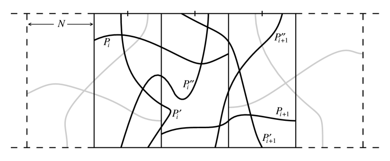
Figure 6. The setting of the proof of Proposition 4.8, case $\alpha_{N}=\lfloor N/2\rfloor$. The collection of paths shown suffices to ensure a left-to right crossing through the four shown translates of $B(N)$. The key points to observe are that $P_{i}$ intersects both $P_{i}^{\prime}$ and $P_{i}^{\prime\prime}$ while $P_{i}^{\prime\prime}$ intersects $P_{i+1}^{\prime}$, for each $i$.

It follows that the graph union of the seven triplets of paths contains a left-to-right crossing of the rectangle $S$ and, by Lemma 2.4, we thus get

$$R_{{\text{\rm LR}};S,{\chi_{M}}}\leq\sum_{i=1}^{7}\Bigl{(}R_{S_{i},\chi_{M}}(\mathcal{P}_{i})+R_{S_{i},\chi_{M}}(\mathcal{P}_{i}^{\prime})+R_{S_{i},\chi_{M}}(\mathcal{P}_{i}^{\prime\prime})\Bigr{)}.$$ (4.42)

In light of the definition (4.20) (and, for simplicity of computation, restricting $\mathcal{P}_{i}$ to paths that terminate only at the top $[\alpha_{N},N]$ portion of the right boundary), (4.40) and the FKG inequality now give (4.39) with $C_{3}:=21C_{3}^{\prime}$ and $c_{0}:=10^{-63}$. ∎

Proof of Proposition 4.8, case $\alpha_{N}<\lfloor N/2\rfloor$. Here, in addition to (4.29) which, as before, we bring to the form (4.40), we will also need (4.30) — this is why we need $\alpha_{N}<\lfloor N/2\rfloor$ — which we extend using Corollary 3.8 and Lemma 4.7 to the form

$$\mathbb{P}\bigl{(}R_{S,[0,\alpha_{N}],\chi_{M}}\leq C_{3}^{\prime\prime}\mathrm{e}^{\hat{\fraktura c}\log\log M}\bigr{)}\geq 0.01$$ (4.43)

for some $C_{3}^{\prime\prime}\in(0,\infty)$, all $N\geq N_{0}$ and all translates $S$ of $B(N)$ such that $S\subseteq B(M/2)$. The same bound holds also for all rotations and reflections of these quantities.

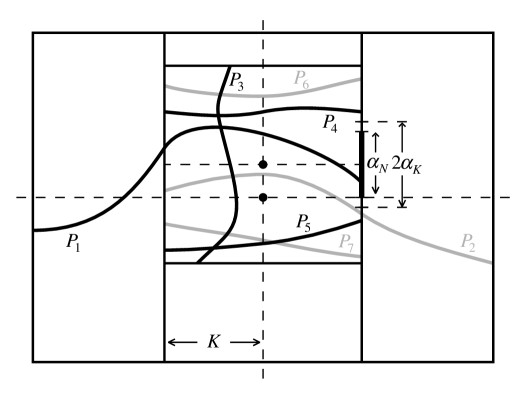
Figure 7. An illustration of the geometric setting underlying the key argument in the proof of Proposition 4.8, case $\alpha_{N}<\lfloor N/2\rfloor$. Here $K:=\lfloor 4N/7\rfloor$ and $\alpha_{N}\leq 2\alpha_{K}$. Examples of paths $P_{1}\in\mathcal{P}_{1}$, $P_{3}\in\mathcal{P}_{3}$, $P_{4}\in\mathcal{P}_{4}$ and $P_{5}\in\mathcal{P}_{5}$ are shown in black. Together with any choice of paths $P_{2}\in\mathcal{P}_{2}$, $P_{6}\in\mathcal{P}_{6}$ and $P_{7}\in\mathcal{P}_{7}$ (shown in gray), these enforce a left-to-right crossing of the rectangle. We note that, although in the above drawing one of $P_{5}$ and $P_{7}$ can be dropped without changing the overall effect, all the depicted paths are generally needed to achieve the desired crossing.

Abbreviate $K:=\lfloor 4N/7\rfloor$ and note that $K<N<2K$ for $N$ large enough. Let us first deal with $S$ being a translate of the rectangle $([-N,3N-2K]\times[-N,N])\cap\mathbb{Z}^{2}$ by some $x\in\mathbb{Z}^{2}$ subject to the restriction $S\subseteq B(4K)$. Consider the squares

$$S_{1}:=x+B(N),\quad S_{2}:=x+2(N-K)e_{1}+B(N)$$ (4.44)

and

$$S_{3}:=x+(N-K)e_{1}+\alpha_{K}e_{2}+[-K,K]^{2}\cap\mathbb{Z}^{2}$$ (4.45)

and note that $S_{1}\cup S_{2}=S$ and $S_{3}\subseteq S_{1}\cap S_{2}$; see Fig. 6. Define the following collections of paths: First, let $\mathcal{P}_{1}$ be all paths in $S_{1}$ from the left side to the $[0,\alpha_{N}]$ portion of the right side. Similarly, let $\mathcal{P}_{2}$ be all paths in $S_{2}$ from the $[0,\alpha_{N}]$ portion of the left side to the right side of $S_{2}$. Next we define the following collections of paths in $S_{3}$:

1. the set $\mathcal{P}_{3}$ of all paths from the top to the bottom sides of $S_{3}$,

2. the set $\mathcal{P}_{4}$ of all paths from the left side of $S_{3}$ to the $[\alpha_{K},K]$ portion of the right side,

3. the set $\mathcal{P}_{5}$ of all paths from the left side of $S_{3}$ to the $[-K,-\alpha_{K}]$ portion of the right side,

4. the set $\mathcal{P}_{6}$ of all paths from the $[\alpha_{K},K]$ portion of the left side of $S_{3}$ to the right side, and

5. the set $\mathcal{P}_{7}$ of all paths from the $[-K,-\alpha_{K}]$ portion of the left side of $S_{3}$ to the right side.

The key point is that, thanks to the assumption $\alpha_{N}\leq 2\alpha_{K}$, for any choice of paths $P_{i}\in\mathcal{P}_{i}$, the graph union of these paths will contain a left-to-right path crossing $S$; see Fig. 6. By Lemma 2.4,

$$R_{{\text{\rm LR}},S,\chi_{M}}\leq\sum_{i=1}^{7}R_{S_{i},\chi_{M}}(\mathcal{P}_{i}),$$ (4.46)

where $S_{4}=\dots=S_{7}:=S_{3}$. From here we get (4.39) for all $2(2N-K)\times 2N$ rectangles $S\subseteq B(M/2)$ with $C_{3}:=21\max\{C_{3}^{\prime},C_{3}^{\prime\prime}\}$ and $c_{0}:=10^{-14}$.

In order to prove the desired claim, consider a translate $S$ of $B(4N,N)$ by $x\in\mathbb{Z}^{2}$ entirely contained in $B(M/2)$ and note that, letting $k:=\lceil\frac{4N}{N-K}\rceil$, and we can cover $S$ by the family of rectangles $S_{0}^{\prime},\dots,S_{k}^{\prime}$ and $S_{1}^{\prime\prime},\dots,S_{k-1}^{\prime\prime}$ defined as follows:

$$S_{j}^{\prime}:=x_{j}+\bigl{(}[0,2(2N-K)]\times[-N,N]\bigr{)}\cap\mathbb{Z}^{2},\quad j=0,\dots,k,$$ (4.47)

where $x_{j}:=x+2(N-K)je_{1}$ for all $j=0,\dots,k-1$ and $x_{k}:=x+[8N-2k(N-K)]e_{1}$, which ensures that all $S_{i}^{\prime}$ lie inside $S$ (and thus inside $B(M/2)$), and

$$S_{j}^{\prime\prime}:=y_{j}+\bigl{(}[-N,N]\times[0,2(2N-K)]\bigr{)}\cap\mathbb{Z}^{2},\quad j=1,\dots,k-1,$$ (4.48)

where $y_{j}-x_{j}$ are such that all $S_{j}^{\prime\prime}$ lie in $B(M/2)$ (this is possible because $2(2N-K)<16N$) and such that $S_{j}^{\prime}\cap S_{j}^{\prime\prime}\subseteq S_{j+1}^{\prime}$ for each $j=1,\dots,k-1$. Assuming each $S_{j}^{\prime}$ and $S_{j}^{\prime\prime}$ contains a path connecting the shorter sides of the rectangle, the graph union of these paths then contains a left-to-right crossing of $S$. Lemma 2.4 then gives

$$R_{{\text{\rm LR}},S,\chi_{M}}\leq\sum_{j=0}^{k}R_{{\text{\rm LR}},S_{j}^{\prime},\chi_{M}}+\sum_{j=1}^{k-1}R_{{\text{\rm UD}},S_{j}^{\prime\prime},\chi_{M}}\,.$$ (4.49)

In light of our earlier proof of (4.39) for rectangles of dimensions $2N\times 2(2N-K)$, we get (4.39) for $2N\times 8N$ rectangles as well with $C_{3}:=21(2k+1)\max\{C_{3}^{\prime},C_{3}^{\prime\prime}\}$ and $c_{0}=10^{-14(2k+1)}$. ∎

4.4. Bounding the growth of $\alpha_{N}$

It appears that Proposition 4.8 could be more than sufficient for proving uniform upper bound on resistance across rectangles, provided we can somehow guarantee that $N\mapsto\alpha_{N}$ does not grow faster than exponentially with $N$. This is the content of:

Proposition 4.9.

For each $c_{0}\in(0,1)$ and each $C_{3}\in(0,\infty)$, there exists an integer $C_{5}>8$ such that if, for some $N\geq 1$,

$$\mathbb{P}\bigl{(}R_{{\text{\rm LR}};S,{\chi_{16N}}}\leq C_{3}\mathrm{e}^{\hat{\fraktura c}\log\log(16N)}\bigr{)}\geq c_{0}$$ (4.50)

holds for all translates or rotates $S$ of $B(4N,N)$ contained in $B(8N)$, then we have $\alpha_{N^{\prime}}\geq N$ for at least one $N^{\prime}\in\{8N,\dots,C_{5}N\}$.

The proof will be based on the following lemma:

Lemma 4.10.

Suppose that, for some $c_{0},C_{3}\in(0,\infty)$ and some $N\geq 1$, (4.50) holds for all translates and rotates of $B(4N,N)$ contained in $B(8N)$. There are $c_{1}$ and $C_{4}$, depending only on $c_{0}$ and $C_{3}$, respectively, such that whenever $K>2N$ is such that $\alpha_{K}\leq N$ and $M\geq 16K$,

$$\mathbb{P}\bigl{(}R_{{\text{\rm LR}},S,\chi_{M}}\leq C_{4}\mathrm{e}^{\hat{\fraktura c}\log\log M}\bigr{)}\geq c_{1}$$ (4.51)

holds for all translates and rotates of $B(4K,K)$ contained in $B(8K)$.

Figure 8. The geometric setup for the proof of Lemma 4.10. The graph union of paths $P_{1},P_{2},P_{1}^{\prime},\dots,P_{4}^{\prime}$ contains a left-to-right crossing of the $4K\times 2K$-rectangle.

Proof. We will first prove this for rectangles $S$ of the form $B(2K,K)$. Consider the squares $S_{1}:=-Ke_{1}+[-K,K]^{2}\cap\mathbb{Z}^{2}$ and $S_{2}:=Ke_{1}+B(K)$ and let $S_{1}^{\prime},\dots,S_{4}^{\prime}$ be the four maximal rectangles of dimensions $N\times 4N$, labeled counterclockwise starting from the one at the bottom, contained in the annulus $B(2N)\smallsetminus B(N)^{\circ}$. Let $P_{1}$ be a path in $S_{1}$ connecting the left-hand side to the $[0,\alpha_{K}]$ portion of the right-hand side and, similarly, $P_{2}$ is the path in $S_{2}$ connecting the $[0,\alpha_{K}]$-portion of the left-hand side to the right hand side. Let $P_{1}^{\prime},\dots,P_{4}^{\prime}$ be paths (in $S_{1}^{\prime},\dots,S_{4}^{\prime}$, respectively) between the shorter sides of $S_{1}^{\prime},\dots,S_{4}^{\prime}$, respectively. Then the assumption $\alpha_{K}\leq N$ implies that the graph union of $P_{1},P_{2},P_{1}^{\prime},\dots,P_{4}^{\prime}$ contains a path in $S$ connecting the left side to the right side; see Fig. 8. Combining (4.51) with (4.43) (in which $N$ is replaced by $K$), we get the claim for $S$ with $C_{4}:=2C_{3}^{\prime\prime}+4C_{3}$ and $c_{1}:=10^{-4}(c_{0})^{4}$.

To extend this to rectangles $S$ of the form $B(4K,K)$, we note that these can be covered by four translates and two rotates of $B(2K,K)$ such that the existence of a crossing between the shorter sides in each of these rectangles forces a crossing of $S$. Thanks to Lemma 4.7, the desired bound then holds for $S$ as well; we just need to multiply the above $C_{4}$ by $6$ and raise the above $c_{1}$ to the sixth power. ∎

We are now ready to give:

Proof of Proposition 4.9. The proof is by way of contradiction; indeed, we will prove that if such $N^{\prime}$ does not exist, then we will ultimately violate the first inequality in (P2) in Lemma 4.5 for a sufficiently large square. This will be done by showing that a path from the left side of the square $B(N^{\prime})$ to the $[0,\alpha_{N^{\prime}}]$ part of the right side can be re-routed to instead terminate in the $[\alpha_{N^{\prime}},N^{\prime}]$-part of the right side. The re-routing will be achieved by showing existence of a path winding around an annulus of inner “radius” at least $\alpha_{N^{\prime}}$ centered at the point $\mathrm{O}_{N^{\prime}}:=(N^{\prime},0)$.

We will focus on $N^{\prime}$ of the form $N^{\prime}:=b^{n}N$, where $b:=8$ and $n\geq 1$. Fix such an $n$ (and thus $N^{\prime}$) and, for $k=1,\dots,n$, let $B_{n,k}:=\mathrm{O}_{N^{\prime}}+B(b^{k}N)$. Consider also the annulus $A_{n,k}:=\mathrm{O}_{N^{\prime}}+B(4b^{k}N)\smallsetminus B(2b^{k}N)^{\circ}$ and define the conditional field

$$\chi_{4N^{\prime},k;v}:=\chi_{4N^{\prime},v}-\mathbb{E}\biggl{(}\chi_{4N^{\prime},v}\,\bigg{|}\,\sigma\Bigl{(}\chi_{4N^{\prime},u}\colon u\in\bigcup_{n-k\leq j\leq n}\partial B_{n,j}\Bigr{)}\biggr{)}.$$ (4.52)

By the Gibbs-Markov property of the GFF, $\{\chi_{4N^{\prime},k;v}\colon v\in A_{n,k}\}$ has the law of the values on $A_{n,k}$ of the GFF in $B(b^{k+1}N)\smallsetminus B(b^{k}N)^{\circ}$ with Dirichlet boundary condition. Let $R_{A_{n,k};\chi_{4N^{\prime},k}}$ denote the sum of the resistances between the shorter sides of the four maximal rectangles contained in $A_{n,k}$, in the field $\chi_{4N^{\prime},k}$.

Assuming $\alpha_{N^{\prime}}\leq N$, Lemma 4.10 in conjunction with Corollary 3.8 and Lemma 4.7 show that, for some $C^{\prime}_{4}\in(0,\infty)$ and $c_{2}>0$:

$$\mathbb{P}\bigl{(}R_{A_{n,k};\chi_{4N^{\prime},k}}\leq C^{\prime}_{4}\mathrm{e}^{\hat{\fraktura c}\log\log N^{\prime}}\bigr{)}\geq c_{2}\,.$$ (4.53)

Let $m$ be the smallest integer such that $(1-c_{2})^{m}\leq 0.01$, let $C_{1}$ be as in the first inequality in (P2) in Lemma 4.5 and let $\widetilde{C}$ be the constant from Lemma 3.10. Define

$$\widetilde{M}_{n,k}:=\min_{v\in A_{n,k}}\mathbb{E}\biggl{(}\chi_{4N^{\prime},v}\,\bigg{|}\,\sigma\Bigl{(}\chi_{N^{\prime},u}\colon u\in\bigcup_{n-k\leq j\leq n}\partial B_{j,n}\Bigr{)}\biggr{)}.$$ (4.54)

Lemma 3.10 (dealing with the LIL for the sequence $M_{n,k}$) and Lemma 3.11 (dealing with the deviations $\Delta_{n}$) tell us that there is a positive integer $m^{\prime}>100$ satisfying

$$\qquad\mathbb{P}\biggl{(}\#\Bigl{\{}k=1,\dots,m^{\prime}-1\colon\gamma\widetilde{M}_{k,m^{\prime}}\geq 0.5\log\frac{C^{\prime}_{4}}{C_{1}}+\log 5+\widetilde{C}\gamma\sqrt{\log m^{\prime}}\Bigr{\}}<m\biggr{)}\\ \leq 0.01+0.01=0.02\,.\qquad$$ (4.55)

Putting together (4.53), (4.55), the choices of $m$ and $m^{\prime}$ along with Lemmas 3.11 and 4.2 we get for all $N$ such that $c\log\big{(}1+\tfrac{(m^{\prime}+1)\log 8}{\log N}\big{)}\leq\log 5$,

$$\mathbb{P}\big{(}\exists k\in\{1,\dots,m^{\prime}\}\colon R_{A_{k,m^{\prime}};\chi_{C_{5}N}}\geq C_{1}\mathrm{e}^{\hat{\fraktura c}\log\log N}\big{)}\leq 0.02+0.01=0.03\,,$$ (4.56)

where $C_{5}:=8^{m^{\prime}+1}$.

Figure 9. The geometric setting for a key argument in the proof of Proposition 4.9: Once $\alpha_{N}$ is less than the inner radius of the depicted annulus, $R_{B(N)_{\chi}}(\mathcal{P}_{N;[\alpha_{N},N]})$ is bounded by $R_{B(N)_{\chi}}(\mathcal{P}_{N;[0,\alpha_{N}]})$ plus the sum of the resistances between the shorter sides of the four maximal rectangles contained in the annulus.

We are now ready to derive the desired contradiction. Lemma 2.4 gives us that if $\alpha_{N^{\prime}}\leq N$ for all $8N\leq N^{\prime}\leq C_{5}N$, then

$$\mathbb{P}\Bigl{(}R_{B(N^{\prime})_{\chi_{N^{\prime}}}}(\mathcal{P}_{N^{\prime};[\alpha_{N^{\prime}},N^{\prime}]})\leq R_{B(N^{\prime})_{\chi_{N^{\prime}}}}(\mathcal{P}_{N^{\prime};[0,\alpha_{N^{\prime}}]})+C_{1}\mathrm{e}^{\hat{\fraktura c}\log\log N}\Bigr{)}\\ \geq 1-0.03=0.97\,.$$ (4.57)

From the second inequality in (P2) in Lemma 4.5 we have

$$\mathbb{P}\bigl{(}R_{B(N^{\prime})_{\chi_{N^{\prime}}}}(\mathcal{P}_{N^{\prime};[0,\alpha_{N^{\prime}}]})\leq 4\mathrm{e}^{\hat{\fraktura c}\log\log N^{\prime}}\bigr{)}\geq 0.17\,.$$ (4.58)

The last two displays and the FKG imply

$$\mathbb{P}\Bigl{(}R_{B(N^{\prime})_{\chi_{N^{\prime}}}}(\mathcal{P}_{N^{\prime};[\alpha_{N^{\prime}},N^{\prime}]})\leq(4+C_{1})\,\mathrm{e}^{\hat{\fraktura c}\log\log N^{\prime}}\Bigr{)}>0.17\times 0.97>0.16\,.$$ (4.59)

in contradiction with the first inequality in (P2) in Lemma 4.5. The claim follows. ∎

4.5. Resistance across rectangles and annuli

As a consequence of the above arguments, we are now ready to state our first unrestricted general upper bound on the effective resistance across rectangles:

Proposition 4.11.

There are constants $C_{6},c_{3}\in(0,\infty)$ and $N_{1}\geq 1$ such that for all $N\geq N_{1}$, all $M\geq 16N$ and for every translate $S$ of $B(4N,N)$ contained in $B(M/2)$, we have

$$\mathbb{P}\bigl{(}R_{{\text{\rm LR}};S,{\chi_{M}}}\leq C_{6}\mathrm{e}^{\hat{\fraktura c}\log\log(M)}\bigr{)}\geq c_{3}\,.$$ (4.60)

The same applies to $R_{{\text{\rm UD}};S,{\chi_{M}}}$ for translates $S$ of $B(N,4N)$ with $S\subseteq B(M/2)$.

We begin by showing that (4.50) holds (with the same constants) along an exponentially growing sequence of $N$. This is where Proposition 4.8 and Proposition 4.9 come together. Later we use Lemma 2.4 to extend this bound to all the intermediate scales by combining the effective resistances along a sequence of appropriately placed rectangles.

Lemma 4.12.

Let $c_{0}$ and $C_{3}$ be as in Proposition 4.8. There is $c\in(0,\infty)$ and an increasing sequence $\{N_{k}\colon k\geq 1\}$ of positive integers such that, for each $k\geq 1$, we have

$$14N_{k}-1\leq N_{k+1}\leq cN_{k}$$ (4.61)

and the bound

$$\mathbb{P}\bigl{(}R_{{\text{\rm LR}};S,{\chi_{16N_{k}}}}\leq C_{3}\mathrm{e}^{\hat{\fraktura c}\log\log(16N_{k})}\bigr{)}\geq c_{0}$$ (4.62)

holds for all translates $S$ of $B(4N_{k},N_{k})$ contained in $B(8N_{k})$.

Proof. We will construct $\{N_{k}\colon k\geq 1\}$ by induction. Suppose that $N_{1},\dots,N_{k}$ have already been defined. Since (4.62) holds for $N_{k}$, Proposition 4.9 shows the existence of an $L\in[8N_{k},C_{5}N_{k}]$ with $\alpha_{L}\geq N_{k}$. Define a sequence $\{L_{j}\colon j\geq 0\}$ by $L_{0}:=L$ and $L_{j+1}:=\min\{L\in\mathbb{N}\colon\lfloor 4L/7\rfloor=L_{j}\}$ and note that $L_{j}\leq c(7/4)^{j}L$ for some numerical constant $c^{\prime}\in(0,\infty)$. Now if $\alpha_{L_{i+1}}>2\alpha_{L_{i}}$ is true for $i=0,\dots,j-1$, then

$$2^{j}N_{k}\leq 2^{j}\alpha_{L}<\alpha_{L_{j}}\leq L_{j}\leq c^{\prime}(7/4)^{j}L\leq c^{\prime}(7/4)^{j}C_{5}N_{k}.$$ (4.63)

The fact that $7/4<2$ implies that this must fail once $j$ is sufficiently large; i.e., for some $j\in\{0,\dots,C_{5}^{\prime}\}$, where $C_{5}^{\prime}$ depends only on $C_{5}$. We thus let $j\geq 1$ be the smallest such that $\alpha_{L_{j}}\leq 2\alpha_{L_{j-1}}$ and set $N_{k+1}:=L_{j}$. Then (4.61) holds by the inequality on the right of (4.63) and the fact that $N_{k+1}\geq L_{1}\geq(7/4)L-1\geq 14N_{k}-1$. The bound (4.62) is implied by Proposition 4.8.

To start the induction, we just take the above sequence $\{L_{j}\}$ with $L:=1$ and find the first index $j$ for which $\alpha_{L_{j}}\leq 2\alpha_{L_{j-1}}$. Then we set $N_{1}:=L_{j}$ and argue as above. ∎

From here we now conclude:

Proof of Proposition 4.11. Let $\{N_{k}\}$ be the sequence from Lemma 4.12. Invoking Corollary 3.8, the bound (4.62) shows that, for each $M\geq 16N_{k}$ and any translate $S$ of $B(4N_{k},N_{k})$ contained in $B(M/2)$,

$$\mathbb{P}\bigl{(}R_{{\text{\rm LR}};S,{\chi_{M}}}\leq C_{3}^{\prime}\mathrm{e}^{\hat{\fraktura c}\log\log(M)}\bigr{)}\geq c_{0}^{\prime}.$$ (4.64)

holds with some constants $C_{3}^{\prime},c_{0}^{\prime}\in(0,\infty)$ independent of $k$ and $M$. By invariance of the law of $\chi_{M}$ with respect to rotations of $B(M)$, the same holds for the resistance $R_{{\text{\rm UD}};S,{\chi_{M}}}$ for all rotations of $B(4N_{k},N_{k})$ contained in $B(M/2)$.

Now pick $N\geq N_{1}$ and let $k$ be such that $N_{k}\leq N<N_{k+1}$. For $M\geq 16N\geq 16N_{k}$, consider a translate $S$ of $B(4N,N)$ contained in $B(M/2)$. Let $m:=\min\{r\in\mathbb{N}\colon(3r+1)N\geq N_{k+1}\}$; by (4.61) this $m$ is bounded uniformly in $k$. We then find rectangles $S_{i}$, $i=1,\dots,m$ that are translates of $B(4N_{k},N_{k})$ such that $S_{i+1}=3Ne_{1}+S_{i}$ for each $i=1,\dots,m-1$ and are centered along the same horizontal line as $S$ and positioned in such a way that they all lie inside $B(M/2)$. Next we find translates $S_{1}^{\prime},\dots,S_{m-1}^{\prime}$ of $B(N_{k},4N_{k})$ such that $S_{i}\cap S_{i+1}$, which is a translate of $B(N)$, is contained in $S_{i}^{\prime}$ for each $i=1,\dots,m-1$. We can again position these so that $S_{i}^{\prime}\subseteq B(M/2)$ for each $i$.

It is clear from the construction that if, for each $i=1,\dots,m$, we are given a path in $S_{i}$ and, for each $i=1,\dots,m-1$, a path in $S_{i}^{\prime}$ and these paths connect the shorter sides of the rectangle they lie in, then the graph union of all these paths contains a path in $S$ between the left side and right side thereof. Lemma 2.4 then gives

$$R_{{\text{\rm LR}};S,{\chi_{M}}}\leq\sum_{i=1}^{m}R_{{\text{\rm LR}};S_{i},{\chi_{M}}}+\sum_{i=1}^{m-1}R_{{\text{\rm UD}};S^{\prime}_{i},{\chi_{M}}}.$$ (4.65)

All the rectangles lie in $B(M/2)$ and so (4.64) applies to the resistances on the right of (4.65). Lemma 4.7 then readily gives (4.62) with the constants given by $C_{6}:=(2m-1)C_{3}^{\prime}$ and $c_{3}:=(c_{0}^{\prime})^{2m-1}$. ∎

In addition to resistance across rectangles, the proofs in Section 5 will also require an lower bound for resistances across annuli. For $N<M$, let $A(N,M):=B(M)\smallsetminus B(N)^{\circ}$ and denote

$$\partial^{\text{\rm in}}A(N,M):=\partial B(N)\quad\text{\rm and}\quad\partial^{\text{\rm out}}A(N,M):=\partial B(M)^{\circ}$$ (4.66)

Note that $\partial^{\text{\rm in}}A(N,M)\subset A(N,M)$ as well as $\partial^{\text{\rm out}}A(N,M)\subset A(N,M)$. We have:

Lemma 4.13.

There $C_{7},c_{4}\in(0,\infty)$ such that for all large-enough $N$ and $A:=A(N,2N)$,

$$\mathbb{P}\Bigl{(}R_{A_{\chi_{4N}}}(\partial^{\text{\rm in}}A,\partial^{\text{\rm out}}A)\geq C_{7}\mathrm{e}^{-3\hat{\fraktura c}\log\log(4N)}\Bigr{)}\geq c_{4}.$$ (4.67)

Proof. Let $S_{1},S_{2},S_{3},S_{4}$ denote the four maximal rectangles contained in $A$. We assume that the rectangles are labeled clockwise starting from the one on the right. Now observe that every path in $A$ from $\partial^{\text{\rm in}}A$ to $\partial^{\text{\rm out}}A$ contains a path that is contained in, and connects the longer sides of, one of the rectangles $S_{1},S_{2},S_{3},S_{4}$. It follows that

$$R_{A_{\chi_{4N}}}(\partial^{\text{\rm in}}A,\partial^{\text{\rm out}}A)\geq R_{{\text{\rm LR}},S_{1},\chi_{4N}}+R_{{\text{\rm UD}},S_{2},\chi_{4N}}+R_{{\text{\rm LR}},S_{3},\chi_{4N}}+R_{{\text{\rm UD}},S_{4},\chi_{4N}}\,.$$ (4.68)

The claim will follow from the FKG inequality if we can show that, for some $p>0$ and $C_{7}^{\prime}>0$,

$$\mathbb{P}\bigl{(}R_{{\text{\rm LR}},S,\chi_{4N}}\geq C_{7}^{\prime}\mathrm{e}^{-3\hat{\fraktura c}\log\log(4N)}\bigr{)}\geq p$$ (4.69)

holds for all translates $S$ of $([0,N]\times[0,4N])\cap\mathbb{Z}^{2}$ contained in $B(2N)$ and all $N$ sufficiently large. (Indeed, then $c_{4}:=p^{4}$ and $C_{7}:=4C_{7}^{\prime}$.)

We will show this using the duality in Lemma 2.6, but for that we will first need to invoke the decomposition $\chi_{4N}=Y_{4N}+Z_{4N}$ from Lemma 3.13. First, for any $r,A>0$,

$$\mathbb{P}\bigl{(}R_{{\text{\rm LR}},S,\chi_{4N}}\geq r\bigr{)}\geq\mathbb{P}\bigl{(}R_{{\text{\rm LR}},S,Z_{4N}}\geq r/A\bigr{)}-\mathbb{P}\bigl{(}R_{{\text{\rm LR}},S,\chi_{4N}}<AR_{{\text{\rm LR}},S,Z_{4N}}\bigr{)}$$ (4.70)

Passing over to conductances, from Lemma 4.2 we then get, as before,

$$\mathbb{P}\bigl{(}R_{{\text{\rm LR}},S,\chi_{4N}}<AR_{{\text{\rm LR}},S,Z_{4N}}\bigr{)}\leq\frac{1}{A}\mathrm{e}^{\hat{\fraktura c}\log\log(4N)},$$ (4.71)

while the duality in Lemma 2.6 gives, as in the proof of Proposition 4.1,

$$\mathbb{P}\Bigl{(}R_{{\text{\rm LR}},S,Z_{4N}}\,R^{\star}_{{\text{\rm UD}},S,Z_{4N}}\geq\mathrm{e}^{-2\gamma c_{1}}/64\Bigr{)}\geq 1-\epsilon.$$ (4.72)

Finally, we use Lemma 4.2 one more time to get

$$\mathbb{P}\bigl{(}R^{\star}_{{\text{\rm UD}},S,Z_{4N}}\leq\tilde{r}\bigr{)}\geq\mathbb{P}\bigl{(}R_{{\text{\rm UD}},S,\chi_{4N}}\leq\tilde{r}/A\bigr{)}-\frac{1}{A}\mathrm{e}^{\hat{\fraktura c}\log\log(4N)}.$$ (4.73)

If we set $\tilde{r}/A:=C_{6}\mathrm{e}^{\hat{\fraktura c}\log\log(4N)}$, Proposition 4.11 bounds the first probability below by $c_{3}$. Now take $A:=C\mathrm{e}^{3\hat{\fraktura c}\log\log(4N)}$ for $C$ large and work your way back to get (4.69). ∎

4.6. Gaussian concentration and upper bound on point-to-point resistances

To get the tail estimate on the effective resistance in Theorem 1.4, we need to invoke a concentration-of-measure argument for the quantity at hand. Recall the notation $R_{A_{\chi}}(\mathcal{P})$ for the effective resistance in network $A_{\chi}$ restricted to the collection of paths in $\mathcal{P}$.

Proposition 4.14.

Suppose $\chi$ is a Gaussian field on $B(N)$ with $\mathrm{Var}(\chi_{x})\leq c_{1}\log N$ for all $u\in B(N)$ and $c_{1}$ independent of $N$. Let $A_{\chi}$ be a subnetwork of $B(N)_{\chi}$ and let $\mathcal{P}$ be a finite collection of paths within $A$ between some given source and destination. There is a constant $c_{2}\in(0,\infty)$ such that for all $N\geq 1$, all $t\geq 0$ and all $\gamma>0$,

$$\mathbb{P}\Bigl{(}\bigl{|}\log{R_{A_{\chi}}(\mathcal{P})}-\mathbb{E}\log{R_{A_{\chi}}(\mathcal{P})}\bigr{|}\geq t\sqrt{\log N}\Bigr{)}\leq 2\mathrm{e}^{-c_{2}\gamma^{-2}t^{2}}\,.$$ (4.74)

For the proof, we will need:

Lemma 4.15.

Let $A$ be a subnetwork of $B(N)$ and $\mathcal{P}$ be a finite collection of paths within $A$ between some given source and destination. Let $g\colon{\mathbb{R}}^{V(A)}\rightarrow{\mathbb{R}}$ be defined by

$$g(\mathbf{x}):=\max_{\mathbf{q}\in\mathcal{Q}}\log\Big{(}\sum_{P\in\mathcal{P}}\frac{1}{\sum\limits_{e\in P}\mathrm{e}^{-\gamma(x_{e_{-}}+x_{e_{+}})}q_{e,P}}\Big{)}\,,$$ (4.75)

where $\mathcal{Q}$ is the set of all $\mathbf{q}=(q_{e,P})_{e\in E(A),P\in\mathcal{P}}\in{\mathbb{R}}_{+}^{E(A)\times\mathcal{P}}$ such that

$$\sum_{P\in\mathcal{P}}\frac{1}{q_{e,P}}\leq 1\,\text{\rm\ for all }\,e\in E(A)\,.$$ (4.76)

Then $g$ is Lipschitz in the $\ell^{\infty}$ norm on ${\mathbb{R}}^{V(A)}$ with Lipschitz constant $2\gamma$.

Proof. Define a new real-valued function, also denoted by $g$, on ${\mathbb{R}}^{V(A)}\times{\mathbb{R}}_{+}^{E(A)\times\mathcal{P}}$ via

$$g(\mathbf{x},\mathbf{q}):=\log\Big{(}\sum_{P\in\mathcal{P}}\frac{1}{\sum\limits_{e\in P}\mathrm{e}^{-\gamma(x_{e_{-}}+x_{e_{+}})}q_{e,P}}\Big{)}\,.$$ (4.77)

Then for any $\mathbf{q}\in\mathcal{Q}$ and $\mathbf{x},\mathbf{y}\in{\mathbb{R}}^{V(A)}$ it is clear that

$$|g(\mathbf{x},\mathbf{q})-g(\mathbf{y},\mathbf{q})|\leq 2\gamma||\mathbf{x}-\mathbf{y}||_{\infty}\,.$$ (4.78)

Hence $g(\mathbf{x})=\max_{\mathbf{q}\in\mathcal{Q}}g(\mathbf{x},\mathbf{q})$ is $2\gamma$- Lipschitz relative to the $\ell^{\infty}$ norm as well. ∎

Proof of Proposition 4.14. The “standard” Gaussian concentration inequality (see [53, 15] and also Lemma 3.1) states that for any centered Gaussian process $\mathbf{X}:=\{X_{v}\colon v\in A\}$ indexed by points in a finite set $A$ and for any $g\colon{\mathbb{R}}^{A}\to{\mathbb{R}}$ obeying $|g(\mathbf{x})-g(\mathbf{y})|\leq c\|\mathbf{x}-\mathbf{y}\|_{\infty}$ for all $\mathbf{x},\mathbf{y}\in{\mathbb{R}}^{A}$,

$$\mathbb{P}\Bigl{(}\,\bigl{|}g(\mathbf{X})-\mathbb{E}g(\mathbf{X})\bigr{|}\geq\lambda\Bigr{)}\leq 2\mathrm{e}^{-\frac{\lambda^{2}}{2c^{2}\sigma^{2}}}\,,\quad\lambda>0,$$ (4.79)

where $\sigma^{2}:=\max_{v\in A}\mathbb{E}(X_{v}^{2})$. The claim then follows via Lemma 4.15. ∎

We are now ready to give a version of the upper bound in Theorem 1.4, albeit for a network arising from a GFF on a finite subset of $\mathbb{Z}^{2}$:

Lemma 4.16.

There is $c_{1}\in(0,\infty)$ depending only on $\gamma$ and a constant $c^{\prime\prime}\in(0,\infty)$ such that

$$\mathbb{P}\Bigl{(}R_{B(N)_{\chi_{M}}}(u,v)\geq c_{1}(\log M)\,\mathrm{e}^{t\sqrt{\log M}}\Bigr{)}\leq 2c_{1}(\log M)\,\mathrm{e}^{-c^{\prime\prime}t^{2}}$$ (4.80)

holds for all $N\geq 1$, all $M\geq 32N$ and all $t\geq 0$.

Proof. We first derive a similar bound for effective resistances across rectangles by Proposition 4.14 and the estimates on its quantiles given by Proposition 4.11 and Corollary 4.3. Then we use a gluing argument like the one used in the proof of Proposition 4.11 to obtain the required upper bound for point-to-point effective resistances. Let us start with the following observation. Combining Proposition 4.11 with Corollary 4.3, for each $\epsilon>0$ there is $N_{0}^{\prime\prime}=N_{0}^{\prime\prime}(\gamma,\epsilon)$ such that if $N\geq N_{0}^{\prime\prime}$, $M\geq 32N$ and $S$ is a translate of $B(4N,N)$ contained in $B(M/2)$, then we have

$$\mathbb{P}\Bigl{(}\bigl{|}\log R_{{\text{\rm LR}};S,\chi_{2M}}\bigr{|}\leq 2\hat{\fraktura c}\log\log(2M)+\log C_{6}\Bigr{)}\geq\epsilon.$$ (4.81)

Decomposing $\chi_{2M}$ on $B(M)$ into a fine field $\chi_{M}^{f}$ and a coarse field $\chi_{M}^{c}$, the fact that

$$|\log R_{{\text{\rm LR}};S,\chi_{2M}}\bigr{|}\geq|\log R_{{\text{\rm LR}};S,\chi_{M}^{f}}\bigr{|}-2\gamma\max_{u\in S}\bigl{|}\chi_{M}^{c}\bigr{|}$$ (4.82)

along with $\chi_{M}^{f}\overset{\text{\rm law}}{=}\chi_{M}$ shows

$$\mathbb{P}\Bigl{(}\bigl{|}\log R_{{\text{\rm LR}};S,\chi_{M}}\bigr{|}\leq 2\hat{\fraktura c}\log\log(2M)+\log C_{6}+2\tilde{c}\gamma\Bigr{)}\geq\epsilon-\mathbb{P}\Bigl{(}\max_{u\in S}\bigl{|}\chi_{M}^{c}\bigr{|}>\tilde{c}\Bigr{)}.$$ (4.83)

The last probability tends to zero as $\tilde{c}\to\infty$ uniformly in $M\geq 1$ and so, by choosing $\tilde{c}$ large, there is a constant $C_{7}\in(0,\infty)$ such that, for all $N\geq N_{0}^{\prime\prime}$,

$$\mathbb{P}\Bigl{(}\bigl{|}\log R_{{\text{\rm LR}};S,\chi_{M}}\bigr{|}\leq 2\hat{\fraktura c}\log\log(2M)+\log C_{7}\Bigr{)}\geq\epsilon/2$$ (4.84)

holds for all $M\geq 32N$ and all translates of $B(4N,N)$ contained anywhere in $B(M)$.

Since (4.84) gives us an interval of width of order $\log\log M$ where $\bigl{|}\log R_{{\text{\rm LR}};S,\chi_{M}}\bigr{|}$ keeps a uniformly positive mass, the Gaussian concentration in Proposition 4.14 shows that, for some constants $c^{\prime},c^{\prime\prime}\in(0,\infty)$,

$$\mathbb{E}\bigl{|}\log R_{{\text{\rm LR}};S,\chi_{M}}\bigr{|}\leq c^{\prime}\sqrt{\log M}$$ (4.85)

and also

$$\mathbb{P}\Bigl{(}\bigl{|}\log R_{{\text{\rm LR}};S,\chi_{M}}\bigr{|}>t\sqrt{\log M}\Bigr{)}\leq 2\mathrm{e}^{-c^{\prime\prime}t^{2}}$$ (4.86)

hold for every $t\geq 0$. The proof has so far assumed $N\geq N_{0}^{\prime\prime}$; to eliminate this assumption we note that $\mathrm{Var}(\chi_{M,v})\leq\tilde{c}\log M$ uniformly in $v\in B(M)$ and so the union bound gives

$$\mathbb{P}\bigl{(}\max_{v\in S}\bigl{|}\chi_{M,v}|>t\sqrt{\log M}\Bigr{)}\leq 2|S|\mathrm{e}^{-\frac{1}{2}\tilde{c}^{-2}t^{2}}.$$ (4.87)

Since $|S|\leq(4N_{0}^{\prime\prime}+1)^{2}$ while $|\log R_{{\text{\rm LR}};S,\chi_{M}}|$ is at most $2\gamma\max_{v\in S}\bigl{|}\chi_{M,v}|$ times an $N_{0}^{\prime\prime}$-dependent constant, by adjusting $c^{\prime\prime}$ we make (4.86) hold for all $N\geq 1$. Due to rotation symmetry, the same bound holds also for $R_{{\text{\rm UD}};S,\chi_{M}}$ and any translate $S$ of $B(N,4N)$ contained in $B(M)$.

Figure 10. A collection of rectangles $4N\times 2N$ or $2N\times 4N$ rectangles with paths that ensure a connection between two given points at distance order $M\geq 32N$.

Now fix $M\geq 32$ and let $u,v\in B(M)$. Then one can find (see Fig. 10) a collection of rectangles of the form $B(N,4N)$ or $B(4N,N)$ with $32N\leq M$ that are contained in $B(M)$ and satisfy:

1. There are at most $c_{1}\log M$ of such rectangles with $c_{1}\in(0,\infty)$ independent of $M$.

2. If a path is chosen connecting the shorter sides in each of these rectangles, then the graph union of these paths contains a path from $u$ to $v$.

By Lemma 2.4, this construction dominates $R_{B(N)_{\chi_{M}}}(u,v)$ by the sum of the resistances between the shorter sides of these rectangles. The FKG inequality, (4.86) and a union bound then imply

$$\mathbb{P}\Bigl{(}R_{B(N)_{\chi_{M}}}(u,v)\geq c_{1}(\log M)\,\mathrm{e}^{t\sqrt{\log M}}\Bigr{)}\leq 2c_{1}(\log M)\,\mathrm{e}^{-c^{\prime\prime}t^{2}}$$ (4.88)

This is the desired claim. ∎

4.7. Adapting the bounds to the full-plane field

In order to extend Lemma 4.16 to the network with the underlying field $\eta$, we first note:

Lemma 4.17.

Let $\eta$ denote the GFF on $\mathbb{Z}^{2}$ pinned at the origin. There are $C_{1},c_{1}\in(0,\infty)$ and $N_{1}\geq 1$ such that for all $N\geq N_{1}$, all $M\geq 16N$ and for every translate $S$ of $B(4N,N)$ contained in  $B(M/2)$, we have

$$\mathbb{P}\bigl{(}R_{{\text{\rm LR}};S,\eta}\leq C_{1}\mathrm{e}^{2\hat{\fraktura c}\log\log(M)}\bigr{)}\geq c_{1}\,.$$ (4.89)

The same applies to $R_{{\text{\rm UD}};S,{\chi_{M}}}$ for translates $S$ of $B(N,4N)$ with $S\subset B(M/2)$.

Proof. We will assume that $M$ is the minimal integer such that $S\subset B(M/2)$. Note that this means that $M/N$ is bounded. We proceed in two steps, first reducing $\eta$ to the GFF in $\Lambda:=B(M)\smallsetminus\{0\}$ and then relating this field to $\chi_{M}$. Using the Gibbs-Markov property, the field $\eta$ can be written as $\chi_{\Lambda}+\chi^{c}$, where $\chi_{\Lambda}$, the fine field, has the law of the GFF on $\Lambda$ while the coarse field $\chi^{c}$ is $\eta$ conditional on its values outside of  $B(M)$. Now pick an $x\in B(M)\smallsetminus B(M/2)^{\circ}$ such that $x$ is at least $M/6$ lattice steps from both $B(M/2)$ and $B(M)^{\text{\rm c}}$. For any $r,A>0$ we then have

$$\mathbb{P}\bigl{(}R_{{\text{\rm LR}};S,\eta}\leq r\bigr{)} \geq\mathbb{P}\bigl{(}R_{{\text{\rm LR}};S,\eta}\leq r,\,\eta_{x}^{c}\geq 0\bigr{)}$$ (4.90)

$$\geq\mathbb{P}\bigl{(}R_{{\text{\rm LR}};S,\eta_{\Lambda}}\leq r/A,\,\eta^{c}_{x}\geq 0\bigr{)}-\mathbb{P}\bigl{(}R_{{\text{\rm LR}};S,\eta}>AR_{{\text{\rm LR}};S,\eta_{\Lambda}},\,\,\eta^{c}_{x}\geq 0\bigr{)}$$

Noting that both events are increasing functions of $\eta$, for the first probability on the right we get

$$\mathbb{P}\bigl{(}R_{{\text{\rm LR}};S,\eta_{\Lambda}}\leq r/A,\,\eta^{c}_{x}\geq 0\bigr{)}\geq\frac{1}{2}\mathbb{P}\bigl{(}R_{{\text{\rm LR}};S,\eta_{\Lambda}}\leq r/A\bigr{)}$$ (4.91)

using the FKG inequality. For the second probability we set

$$\varphi_{u}:=\eta^{c}_{u}-\frac{\mathrm{Cov}(\eta^{c}_{u},\eta^{c}_{x})}{\mathrm{Var}(\eta^{c}_{x})}\eta^{c}_{x},\qquad u\in B(M/2),$$ (4.92)

and note, since $\mathrm{Cov}(\eta^{c}_{u},\eta^{c}_{x})\geq 0$, we have

$$R_{{\text{\rm LR}};S,\eta}\leq R_{{\text{\rm LR}};S,\eta_{\Lambda}+\varphi}\quad\text{on }\{\eta^{c}_{x}\geq 0\bigr{\}}.$$ (4.93)

But the above definition ensures that $\varphi$ is independent of $\eta^{c}_{x}$ and a calculation using the explicit form of the law of $\eta^{c}$ gives that $\max_{v\in\Lambda}\mathrm{Var}(\varphi_{v})$ is bounded by a constant independent of $M$. Markov’s inequality and (4.6) then bound the last probability in (4.90) by $c^{\prime}/A$ for some constant $c^{\prime}\in(0,\infty)$ independent of $A$ or $M$.

Next let $\mathfrak{g}_{M}\colon\mathbb{Z}^{2}\to[0,1]$ be discrete harmonic on $\Lambda$ with $\mathfrak{g}_{M}(0):=1$ and $\mathfrak{g}_{N}(u):=0$ whenever $u\not\in B(M)$. Let $\tilde{\chi}$ have the law of $\chi_{M}(0)\mathfrak{g}(\cdot)$ but assume that $\tilde{\chi}$ is independent of $\chi_{\Lambda}$. The Gibbs-Markov property shows

$$\tilde{\chi}+\chi_{\Lambda}\overset{\text{\rm law}}{=}\chi_{M}.$$ (4.94)

A direct use of Lemma 4.2 is hampered by the fact that $\mathrm{Var}(\tilde{\chi}(0))$ is of order $\log M$. However, this is not a problem when $S$ is at least distance $\delta M$ from the origin because then $\mathfrak{g}_{N}(x)=O(1/\log M)$. Letting $K:=\lfloor N/3\rfloor$, we now note that each translate $S$ of $B(4N,N)$ contains a translate $\tilde{S}$ of $B(4N,K)$ which is at least distance $N$ from the origin and is aligned with one of the longer side of $S$. Lemma 4.2 then gives, for any $b\in{\mathbb{R}}$,

$$R_{{\text{\rm LR}};\tilde{S},\chi_{\Lambda}+\tilde{\chi}}\geq\mathrm{e}^{-c^{\prime\prime}b}R_{{\text{\rm LR}};\tilde{S},\chi_{\Lambda}}\geq\mathrm{e}^{-c^{\prime\prime}b}R_{{\text{\rm LR}};S,\chi_{\Lambda}},\qquad\text{on }\{\tilde{\chi}(0)\leq b\log N\}$$ (4.95)

for some $c^{\prime\prime}>0$. Hence

$$\mathbb{P}\bigl{(}R_{{\text{\rm LR}};S,\chi_{\Lambda}}\leq r/A\bigr{)}\geq\mathbb{P}\bigl{(}R_{{\text{\rm LR}};\tilde{S},\chi_{\Lambda}+\tilde{\chi}}\leq\mathrm{e}^{-\tilde{c}b}r/A\bigr{)}-\mathbb{P}\bigl{(}\tilde{\chi}(0)>b\log N\bigr{)}.$$ (4.96)

Now set $r:=C_{1}\mathrm{e}^{2\hat{\fraktura c}\log\log(M)}$, $A:=\mathrm{e}^{\hat{\fraktura c}\log\log(M)}$ and pick any $b>0$. Then the last probability in both (4.90) and (4.96) tends to zero as $N\to\infty$, while, as soon as $C_{1}$ is large enough, the first probability on the right of (4.96) is uniformly positive by Proposition 4.11 and a routine use of the FKG inequality (to get us from rectangles of the form $B(4N,K)$ to those with aspect ratio $4$). The claim follows. ∎

Using exactly the same argument as in the proof of Lemma 4.16, we then get:

Corollary 4.18.

Let $\eta$ be the GFF in $\mathbb{Z}^{2}\smallsetminus\{0\}$. There are $C,C^{\prime}\in(0,\infty)$ such that

$$\mathbb{P}\Bigl{(}R_{B(N)_{\eta}}(u,v)\geq C\,\mathrm{e}^{Ct\sqrt{\log N}}\,\Bigr{)}\leq C^{\prime}\mathrm{e}^{-t^{2}}\log N$$ (4.97)

holds for all $N\geq 1$ and all $t\geq 0$.

This is one half of Theorem 1.4; the other half will be shown in Section 5.4.

5. Random walk computations

Here we use the techniques developed earlier in this paper to finally prove our main results. We begin with some preparatory claims; the actual proofs start to appear in Section 5.2.

5.1. Points with moderate resistance to origin

Our proofs will require restricting to subsets of $\mathbb{Z}^{2}$ of points with only a moderate value of the effective resistance to the origin and/or the boundary of a box centered there in. Here we give the needed bounds on cardinalities of such sets.

Lemma 5.1.

Denote $A(N,2N):=B(2N)\smallsetminus B(N)^{\circ}$. For any $\delta>0$, we have

$$\mathbb{P}\biggl{(}\,\sum_{v\in A(N,2N)}\pi_{\eta}(v)\,1_{\{R_{B(N)_{\eta}}(0,v)>\mathrm{e}^{(\log N)^{1/2+\delta}}\}}>N^{\psi(\gamma)}\mathrm{e}^{-(\log N)^{\delta}}\biggr{)}\leq\mathrm{e}^{-(\log N)^{\delta}}$$ (5.1)

as soon as $N$ is sufficiently large.

Proof. Abbreviate, as in (3.15), $g:=2/\pi$. We will proceed by a straightforward first-moment estimate, but first we have to localize the problem to a finite box. Write $\eta=\eta^{f}+\eta^{c}$ where $\eta^{f}$ is the fine field on the box $B(4N)$. Since $\mathrm{Var}(\eta^{c}_{v})\leq\mathrm{Var}(\eta_{v})$, the variance of $\eta^{c}$ is bounded by a constant times $\log N$ uniformly on $B(N)$ and so, combining Corollary 3.8 with a bound at one vertex,

$$\mathbb{P}\Bigl{(}\,\min_{v\in A(N,2N)}\eta_{v}^{c}\leq-(\log N)^{1/2+\delta/2}\Bigr{)}\leq c\mathrm{e}^{-\tilde{c}(\log N)^{\delta}}.$$ (5.2)

On the event when $\eta^{c}\geq-(\log N)^{1/2+\delta/2}$ we have

$$R_{B(N)_{\eta}}(0,v)\leq R_{B(N)_{\eta}^{f}}(0,v)\,\mathrm{e}^{2\gamma(\log N)^{1/2+\delta/2}}$$ (5.3)

and so comparing this with the restriction on the effective resistance in (5.1) we may as well estimate the probability in (5.1) for $\eta$ replaced by $\chi_{4N}$.

Here we will still need to employ a truncation to keep the field $\chi_{4N}$ below its typical maximum scale. The following crude estimate based on a union bound is sufficient,

$$\mathbb{P}\Bigl{(}\,\max_{v\in B(N)}\chi_{4N,v}\geq 2\sqrt{g}\log N+(\log N)^{\delta}\Bigr{)}\leq c\mathrm{e}^{-\tilde{c}(\log N)^{\delta}}$$ (5.4)

for some constants $c,\tilde{c}\in(0,\infty)$. Writing $F_{N}$ for the complementary event and inserting $F_{N}$ in the probability in (5.1) with $\eta$ replaced by $\chi_{4N}$, Markov’s inequality bounds the result by

$$N^{-\psi(\gamma)}\mathrm{e}^{(\log N)^{\delta}}\sum_{v\in A(N,2N)}\mathbb{E}\Bigl{(}\pi_{\chi_{4N}}(v)1_{\{R_{B(N)_{\chi_{4N}}}(0,v)>\mathrm{e}^{(\log N)^{1/2+\delta}}\}}\,\Big{|}\,F_{N}\Bigr{)}\,.$$ (5.5)

Now $\eta\mapsto\pi_{\eta}(v)$ is increasing while $\{R_{B(N)_{\eta}}(0,v)>\mathrm{e}^{(\log N)^{\delta}}\}$ is a decreasing event. Since the conditioning on $F_{N}$ preserves the FKG inequality, the quantity in (5.5) is no larger than

$$\frac{1}{\mathbb{P}(A_{N})^{2}}N^{-\psi(\gamma)}\mathrm{e}^{(\log N)^{\delta}}\sum_{v\in B(N)}\mathbb{E}\bigl{(}\pi_{\chi_{4N}}(v);\,F_{N}\bigr{)}\mathbb{P}\Bigl{(}R_{B(N)_{\chi_{4N}}}(0,v)>\mathrm{e}^{(\log N)^{1/2+\delta}}\Bigr{)}.$$ (5.6)

Corollary 4.18 bounds the last probability by $\mathrm{e}^{-\tilde{c}(\log N)^{2\delta}}$ so we just have to compute the sum of the expectations of $\pi_{\eta_{4N}}(v)$’s.

Pick a pair of nearest neighbors $u$ and $v$, with $v\in A(N,2N)$, and let $X:=\chi_{4N,u}+\chi_{4N,v}$. Disregarding the event $F_{N}$, a moment computation using $\mathrm{Var}(\chi_{4N,v})\leq g\log N+c$ for $v\in A(N,2N)$ shows

$$\mathbb{E}\bigl{(}\mathrm{e}^{\gamma X}\bigr{)}=\mathrm{e}^{\frac{1}{2}\gamma^{2}\mathrm{Var}(X)}\leq cN^{2\gamma^{2}g},\qquad v\in A(N,2N).$$ (5.7)

On the other hand, a change of measure argument gives

$$\mathbb{E}\bigl{(}\mathrm{e}^{\gamma X};F_{N}\bigr{)} \leq\mathrm{e}^{\frac{1}{2}\gamma^{2}\mathrm{Var}(X)}\mathbb{P}\Bigl{(}X\leq 4\sqrt{g}\log N+2(\log N)^{\delta}-\gamma\mathrm{Var}(X)\Bigr{)}$$ (5.8)

$$\leq cN^{2\gamma^{2}g}\,\mathbb{P}\Bigl{(}X\leq 4(\sqrt{g}-\gamma g)\log N+3(\log N)^{\delta}\Bigr{)}$$

For $\gamma>\gamma_{\text{\rm c}}:=1/\sqrt{g}$, the probability itself decays as $N^{-2(1-\gamma/\gamma_{\text{\rm c}})^{2}}\mathrm{e}^{c^{\prime}(\log N)^{\delta}}$. Invoking the definition of $\psi(\gamma)$ in (1.5), the inequalities (5.7–5.8) thus give

$$\mathbb{E}\bigl{(}\pi_{\chi_{4N}}(v);\,F_{N}\bigr{)}\leq cN^{\psi(\gamma)-2}\mathrm{e}^{c^{\prime}(\log N)^{\delta}},\qquad v\in A(N,2N).$$ (5.9)

Summing over $v\in A(N,2N)$, the claim follows. ∎

Consider now the set

$$\Xi_{N}:=\{0\}\cup\Bigl{\{}v\in A(N,2N)\colon R_{B(4N)_{\eta}}(0,v)\leq\mathrm{e}^{(\log T)^{1/2+\delta}}\Bigr{\}}.$$ (5.10)

With the help of the above lemma we then show:

Lemma 5.2.

For each $\delta>0$, there is $c>0$ such that for all $N$ sufficiently large,

$$\mathbb{P}\Bigl{(}\,\pi_{\eta}(\Xi_{N})\leq N^{\psi(\gamma)}\mathrm{e}^{-(\log N)^{\delta}}\Bigr{)}\leq\frac{c}{(\log N)^{2}}.$$ (5.11)

Proof. In light of Lemma 5.1, it suffices to show that

$$\mathbb{P}\biggl{(}\,\sum_{v\in A(N,2N)}\pi_{\eta}(v)\,\leq 3N^{\psi(\gamma)}\mathrm{e}^{-(\log N)^{\delta}}\biggr{)}\leq\frac{c}{(\log N)^{2}}.$$ (5.12)

Thanks to the Gibbs-Markov property, it actually suffices to show this (with $\delta$ replaced by $\delta/2$) for $\eta$ replaced by $\chi_{N}$ and $A(N,2N)$ replaced by a box $B(N)$. (Indeed, we just need to take a translate $B$ of $B(N)$ with $B\subset A(N,2N)$ and then use the Gibbs-Markov property on a translate of $B(\lfloor 3N/2\rfloor)$ centered at the same point as $B$. The contribution of the coarse field is estimated using Corollary 3.8.)

The argument for (5.12) is different depending on the relation between $\gamma$ and $\gamma_{\text{\rm c}}$. For $\gamma\geq\gamma_{\text{\rm c}}$ we use that the maximum of the GFF has doubly-exponential lower tails (see [25]). Invoking the Gibbs-Markov property we then conclude that, with probability at least $\mathrm{e}^{-(\log N)^{c}}$, for some $c>0$, there is at least one point $u$ where

$$\chi_{N,u}\geq 2\sqrt{g}\log N-\hat{\fraktura c}\log\log N$$ (5.13)

for some large enough $C>0$. As $\chi_{N,u}-\chi_{N,v}$, for $u$ and $v$ neighbors, have bounded (in fact, stationary) variances, a union bound shows that (5.13) will hold also for the neighbors of $u$. On this event, and denoting by $v$ a neighbor of $u$,

$$\sum_{v\in B(N)}\pi_{\chi_{N}}(v)\geq\mathrm{e}^{\gamma(\chi_{N,u}+\chi_{N,v})}=N^{4\sqrt{g}\gamma}\mathrm{e}^{-c^{\prime}\log\log N}.$$ (5.14)

Since $4\sqrt{g}\gamma=4(\gamma/\gamma_{\text{\rm c}})$ equals $\psi(\gamma)$ for $\gamma\geq\gamma_{\text{\rm c}}$, we are done here.

Concerning $\gamma<\gamma_{\text{\rm c}}$, here we will apply Theorem 3.12 for $\alpha:=\gamma/\gamma_{\text{\rm c}}$. Recall the notation $\mathcal{A}_{N,\alpha}$ for the level set in (3.52). A straightforward computation using the explicit form of the Gaussian probability density shows

$$\mathbb{P}\bigl{(}x\in\mathcal{A}_{N,\alpha}\bigr{)}\geq\frac{c}{\log N}\,N^{-2\alpha^{2}},$$ (5.15)

and so $\mathbb{E}(|\mathcal{A}_{N,\alpha}|)\geq cN^{\psi(\gamma)}/\log N$. Theorem 3.12 ensures that $|\mathcal{A}_{N,\alpha}|\geq\delta\mathbb{E}(|\mathcal{A}_{N,\alpha}|)$ occurs with probability $O(\delta^{c})$. This statements permits even setting $\delta:=1/(\log N)^{c^{\prime}}$, whereby the claim readily follows. ∎

We also record an upper estimate on the total volume of $\pi_{\eta}$:

Lemma 5.3.

For any $\delta>0$, we have

$$\mathbb{P}\biggl{(}\,\,\sum_{v\in B(N)}\pi_{\eta}(v)\,>N^{\psi(\gamma)}\mathrm{e}^{(\log N)^{\delta}}\biggr{)}\leq\mathrm{e}^{-(\log N)^{\delta}}$$ (5.16)

as soon as $N$ is sufficiently large.

Proof. This follows directly from the Markov inequality and the calculations in the formulas (5.7–5.8). ∎

5.2. Upper bound on heat-kernel and exit time

The starting point of our proofs is an upper bound on the return probability for the random walk. We remark that numerous methods exist in the literature to derive such bounds. Some of these are based on geometric properties of the underlying Markov graph such as isoperimetry and volume growth, others are based on resistance estimates. The most natural approach to use would be that of [3] (see also [37]); unfortunately, this does not seem possible due to our lack of required uniform control of the resistance growth. Instead, we base our presentation on the general strategy outlined in [40, Chapter 21.5]. We begin by restating, and proving, one half of Theorem 1.1:

Lemma 5.4.

For each $\delta>0$,

$$\lim_{T\to\infty}\,\mathbb{P}\Bigl{(}P_{\eta}^{0}(X_{2T}=0)\leq\mathrm{e}^{(\log T)^{1/2+\delta}}T^{-1}\Bigr{)}=1\,.$$ (5.17)

Proof. Pick $\delta>0$ and a large integer $T$, and recall the notation $\Xi_{T}$ for the set in (5.10). Consider the random walk $\{\widetilde{X}_{t}\colon t\geq 0\}$ on the network $B(4T)_{\eta}$; this walk starts at $0$ and moves around $B(4T)$ indefinitely using the transition probabilities (1.7) that are modified on the boundary of $B(4T)$ so that jumps outside $B(4T)$ are suppressed. Let $\{Y_{t}\colon t\geq 0\}$ record the successive visits of $\widetilde{X}$ to $\Xi_{T}$. Then $Y$ is a Markov chain on $\Xi_{T}$ with stationary distribution

$$\nu(x):=\frac{\pi_{\eta}(x)}{\pi_{\eta}(\Xi_{T})}.$$ (5.18)

Let $\tau_{0}:=0$, $\tau_{1}$, $\tau_{2}$, etc be the times of the successive visits of $Y$ to $0$. Define

$$\hat{\sigma}:=\inf\bigl{\{}k\geq 1\colon\tau_{k}\geq T\,\,\text{and}\,\,Y_{k}=0\bigr{\}}.$$ (5.19)

Then we have

$$(T/2)\cdot P^{0}(\widetilde{X}_{T}=0) \leq E^{0}\Bigl{(}\,\,\sum_{t=0}^{T-1}\,1_{\{\widetilde{X}_{t}=0\}}\Bigr{)}$$ (5.20)

$$\leq E^{0}\Bigl{(}\,\,\sum_{k=0}^{T-1}\,1_{\{Y_{k}=0\}}\Bigr{)}\leq E^{0}\Bigl{(}\,\,\sum_{k=0}^{\hat{\sigma}-1}\,1_{\{Y_{k}=0\}}\Bigr{)},$$

where the first inequality comes from the monotonicity of $2T\mapsto P^{0}(\widetilde{X}_{2T}=0)$ (see, e.g., [40, Proposition 12.8]) and the second inequality reflects the fact that $0\in\Xi_{T}$. Since $Y_{\hat{\sigma}}=0$, by, e.g., [40, Lemma 10.5] we have

$$E^{0}\Bigl{(}\,\sum_{k=0}^{\hat{\sigma}-1}\,1_{\{Y_{k}=x\}}\Bigr{)}=E^{0}(\hat{\sigma})\nu(x).$$ (5.21)

(This is proved by noting that the object on the left is a stationary measure for the walk $Y$ of total mass $E^{0}(\hat{\sigma})$.) By conditioning on $Y_{T}$ we further estimate

$$E^{0}(\hat{\sigma})\leq T+\max_{u\in\Xi_{T}}E^{u}(\sigma_{0}),$$ (5.22)

where $\sigma_{0}:=\inf\{k\geq 0\colon Y_{k}=0\}$ and note that

$$E^{u}(\sigma_{0})\leq\pi_{\eta}(\Xi_{T})\,R_{B(4T)_{\eta}}(0,u)\leq\pi_{\eta}(\Xi_{T})\,\mathrm{e}^{(\log T)^{1/2+\delta}},\qquad u\in\Xi_{T},$$ (5.23)

by the commute-time identity (usually attributed to [21] but appearing already in [18]; see also [42, Corollary 2.21]). Combining this with (5.20–5.21) and (5.18) we then get

$$P^{0}(\widetilde{X}_{T}=0)\leq\frac{1}{T}\,\pi_{\eta}(0)\,\mathrm{e}^{(\log T)^{1/2+\delta}},$$ (5.24)

which proves (5.17) because, due to the jumps being only to nearest neighbors, the walk $\widetilde{X}$ coincides with the walk $X$ up to time at least $4T$. ∎

This now permits to give:

Proof of Theorem 1.3. A standard calculation based on reversibility and the Cauchy-Schwarz inequality yields

$$P^{0}(X_{2T}=0) \geq\sum_{x\in B(N)}P^{0}(X_{T}=x)P^{x}(X_{T}=0)$$ (5.25)

$$=\pi_{\eta}(0)\sum_{x\in B(N)}\frac{P^{0}(X_{T}=x)^{2}}{\pi_{\eta}(x)}\geq\pi_{\eta}(0)\frac{P^{0}\bigl{(}X_{T}\in B(N)\bigr{)}^{2}}{\pi_{\eta}\bigl{(}B(N)\bigr{)}}.$$

Invoking the upper bound on the heat-kernel and Lemma 5.3, we get that with probability tending rapidly to one as $N$ and $T$ tend to infinity, we have

$$P^{0}\bigl{(}X_{T}\in B(N)\bigr{)}\leq\Bigl{[}\frac{1}{T}\mathrm{e}^{(\log T)^{1/2+\delta}}\,N^{\psi(\gamma)}\mathrm{e}^{(\log N)^{\delta}}\Bigr{]}^{1/2}\,.$$ (5.26)

Setting $T:=N^{\psi(\gamma)}\mathrm{e}^{(\log N)^{1/2+2\delta}}$ gives the desired claim. ∎

The same conclusion could in fact be inferred from the following claim which constitutes one half of Theorem 1.2:

Lemma 5.5.

For each $\delta>0$ and all $N$ sufficiently large,

$$\mathbb{P}\Bigl{(}E^{0}(\tau_{B(N)^{\text{\rm c}}})>N^{\psi(\gamma)}\mathrm{e}^{(\log N)^{1/2+\delta}}\Bigr{)}\leq\mathrm{e}^{-(\log N)^{\delta}}.$$ (5.27)

Proof. By the hitting time identity (or, alternatively, the commute time identity)

$$E^{0}(\tau_{B(N)^{\text{\rm c}}})\leq R_{B(N+1)_{\eta}}\bigl{(}0,\partial B(N)\bigr{)}\pi_{\eta}\bigl{(}B(N)\bigr{)}$$ (5.28)

The claim then follows from Corollary 4.18 and Lemma 5.3. ∎

5.3. Bounding the voltage from below

We now move to the proofs of the required lower bounds. Here the focus will be directed to the expected exit time which we write using the hitting time identity as

$$E^{0}(\tau_{B(N)^{\text{\rm c}}})=R_{B(N+1)_{\eta}}\bigl{(}0,\partial B(N)\bigr{)}\sum_{v\in B(N)}\pi_{\eta}(v)\phi(v),\,$$ (5.29)

where, using our convention that $\partial B(N)$ is the external boundary of $B(N)$,

$$\phi(v):=P^{v}(\tau_{0}<\tau_{\partial B(N)})$$ (5.30)

is the electrostatic potential, a.k.a. voltage, in  $B(N)$ with $\phi(0)=1$ and $\phi$ vanishing on $\partial B(N)$. Estimating (5.29) from below naturally requires finding a sufficiently good lower bound on $\phi$. The idea is to recast the problem using a simple electric network and invoke suitable effective resistance estimates. The following computation will be quite useful:

Lemma 5.6.

Consider a resistor network with three nodes, $\{1,2,3\}$, and for each $i,j$ let $c_{ij}$ denote the conductance of the edge $(i,j)$. Let $R_{ij}$ denote the effective resistance between node $i$ and node $j$. Then,

$$\frac{c_{12}}{c_{12}+c_{13}}=\frac{R_{13}+R_{23}-R_{12}}{2R_{23}}.$$ (5.31)

Proof. By the Parallel and Series Laws we get,

$$R_{12}=\frac{1}{c_{12}+(c_{13}^{-1}+c_{23}^{-1})^{-1}}.$$ (5.32)

Computing $R_{13}$ and $R_{23}$ in a similar way and plugging them into the right hand side of (5.31), we deduce the claim. ∎

Using this lemma we then get:

Corollary 5.7.

For any $v\in B(N)\smallsetminus\{0\}$ and $\phi$ as above,

$$\quad 2R_{B(N+1)_{\eta}}\bigl{(}0,\partial B(N)\bigr{)}\phi(v)\\ =R_{B(N+1)_{\eta}}\bigl{(}0,\partial B(N)\bigr{)}+R_{B(N+1)_{\eta}}\bigl{(}v,\partial B(N)\bigr{)}-R_{B(N+1)_{\eta}}(0,v).\quad$$ (5.33)

Proof. As $v\not\in\{0\}\cup\partial B(N)$, we may apply the network reduction principle to represent the problem on an effective network of three nodes, with node $1$ labeling $v$, node $2$ marking the origin and node $3$ standing for $\partial B(N)$. Since $\phi$ is harmonic on $B(N)\smallsetminus\{0\}$, it is also harmonic on the effective network. But there $\phi(v)$ is just the probability that the random walk at $v$ jumps right to $0$ in the first step. Using conductances, this probability is exactly the expression on the left of (5.31). Plugging in the effective resistances, the claim follows. ∎

A key point is to bound the expression involving effective resistances on the right of (5.33) from below. This is the subject of:

Proposition 5.8.

Let $D_{N,\eta}(v)$ denote the difference on the right of (5.33), i.e.,

$$D_{N,\eta}(v):=R_{B(N+1)_{\eta}}\bigl{(}0,\partial B(N)\bigr{)}+R_{B(N+1)_{\eta}}\bigl{(}v,\partial B(N)\bigr{)}-R_{B(N+1)_{\eta}}(0,v).$$ (5.34)

For any $\delta\in(0,1)$, we then have

$$\lim_{N\to\infty}\,\mathbb{P}\Bigl{(}\,\,\min_{v\in B(\lfloor N\mathrm{e}^{-(\log N)^{\delta}}\rfloor)}\,\,D_{N,\eta}(v)\geq\log N\Bigr{)}=1.$$ (5.35)

The main idea behind the proof is to find an annulus between $B_{N}$ and $B(\lfloor N\mathrm{e}^{-(\log N)^{\delta}}\rfloor)$ with high probability which provides a “shortcut” for diverting the flow from 0 to $v$. To this end we recall the annulus decomposition of the GFF from Section 3.2. Let $b:=8$ and for a given $N\geq 1$ and $n\in\mathbb{N}$, set $N^{\prime}:=b^{n}N$. Define the annuli

$$A^{\prime}_{n,k}:=B(b^{n-k+1}N)\smallsetminus B(b^{n-k}N)^{\circ},\qquad k=1,\dots,n-1.$$ (5.36)

and

$$A_{n,k}:=B(4b^{n-k}N)\smallsetminus B(2b^{n-k}N)^{\circ},\qquad k=1,\dots,n-1.$$ (5.37)

Note that $A_{n,k}\subset A^{\prime}_{n,k}$. Write $\eta=\eta^{c}+\chi_{2N^{\prime}}$, where $\eta^{c}$ is the coarse field on $B(2N^{\prime})$ and $\chi_{2N^{\prime}}$ is the corresponding fine field. Denote

$$\Delta^{\prime}:=\max_{v\in B(N^{\prime})}|\eta^{c}_{v}|.$$ (5.38)

Define $M_{n,k}$ as in (3.37) and for $1\leq\ell<m\leq n$ let

$$\Delta_{\ell,m}:=\max_{k=\ell,\dots,m-1}\,\,\max_{v\in A_{n,k}}\,\Bigl{|}M_{n,k}-\mathbb{E}\bigl{(}\chi_{N^{\prime},v}\,\big{|}\,\chi_{N^{\prime},v}:v\in{\textstyle\bigcup_{n\geq j\geq n-k}}\partial B(b^{j}N)\bigr{)}\Bigr{|}.$$ (5.39)

(Both objects are measurable with respect to $\eta$.) Similarly to Lemma 3.11 we get

$$\mathbb{P}\Bigl{(}\Delta_{\ell,m}\geq\widetilde{C}\sqrt{m-\ell}\,\Bigr{)}\leq\frac{1}{(m-\ell)^{2}}$$ (5.40)

as soon as $m-\ell$ is sufficiently large.

Let $\chi_{k,v}^{f}$ denote the fine field on $A_{n,k}^{\prime}$,

$$\chi_{k,v}^{f}:=\mathbb{E}\Bigl{(}\chi_{2N^{\prime},v}\,\Big{|}\,\chi_{2N^{\prime},u}\colon u\in\partial A_{n,k}\Bigr{)},\qquad v\in A_{n,k},$$ (5.41)

(we think of $\chi_{k}^{f}$ as set to zero outside $A^{\prime}_{n,k}$) and $\chi_{k}^{c}:=\chi_{2N^{\prime}}-\chi_{k}^{f}$ be the corresponding coarse field. The definitions ensure

$$\max_{k=\ell,\dots,m}\,\max_{v\in A_{n,k}}\,\bigl{|}\eta_{v}-(\chi_{k,v}^{f}+M_{n,k})\bigr{|}\leq\Delta_{\ell,m}+\Delta^{\prime}.$$ (5.42)

Note also that $M_{n,k}$ and $\chi_{k^{\prime}}^{f}$ are independent as long as $k\geq k^{\prime}$.

Next recall that $R_{A,\eta}$, for $A$ an annulus in $\mathbb{Z}^{2}$, denotes the sum of the effective resistances in network $A_{\eta}$ between the shorter sides of the four maximal rectangles contained in $A$. Recall also that $R_{A,\eta}(\partial^{\text{\rm in}}A,\partial^{\text{\rm out}}A)$ denotes the effective resistance in $A_{\eta}$ between the inner and outer boundaries of annulus $A$. We define the events:

$$\mathcal{E}_{n,k}^{\star}:=\Bigl{\{}R_{A_{n,k},\chi_{k}^{f}}(\partial^{\text{\rm in}}A_{n,k},\partial^{\text{\rm out}}A_{n,k})\geq\mathrm{e}^{-3\hat{\fraktura c}\log\log(b^{-k}N^{\prime})}\Bigr{\}}\\ \cap\Bigl{\{}M_{n,k}\leq-C^{\star}\sqrt{k\log\log(k)}\Bigr{\}}$$ (5.43)

and

$$\mathcal{E}_{n,k}^{\star\star}:=\Bigl{\{}R_{A_{n,k},\chi_{k}^{f}}\leq\mathrm{e}^{\hat{\fraktura c}\log\log(b^{-k}N^{\prime})}\Bigr{\}}\cap\Bigl{\{}\min_{v\in A_{n,k}}\eta_{k,v}^{c}\geq-\log\log(N^{\prime})\Bigr{\}}.$$ (5.44)

Here $\hat{\fraktura c}$ is the constant Proposition 4.1 and $C^{\star}$ is fixed via:

Lemma 5.9.

For each $\delta>0$ there are $n_{0}\geq 1$, $N_{0}\geq 1$, $c_{1}\in(0,\infty)$ such that one can choose $C^{\star}\in(0,\infty)$ in the definitions of $\mathcal{E}_{n,k}^{\star}$ and $\mathcal{E}_{n,k}^{\star\star}$ so that, for all $N\geq N_{0}$ and all $n\geq n_{0}$,

$$\mathbb{P}\Bigl{(}\exists k^{\star},k_{\star}\colon\mathrm{e}^{\sqrt{\log n}}<k^{\star}<k_{\star}<n,\,\,\mathcal{E}_{n,k^{\star}}^{\star}\cap\mathcal{E}_{n,k_{\star}}^{\star\star}\text{\rm\ occurs}\Bigr{)}\geq 1-\frac{c_{1}}{\log\log n}.$$ (5.45)

Proof. Abbreviate by $E_{k}^{\star}$ the first event on the right of (5.43). This event is measurable with respect to $\chi_{k}^{f}$ and so $\{E_{k}\colon k=1,\dots,n\}$ are independent. By Lemma 4.13, $\mathbb{P}(E_{k}^{\star})\geq p$ holds for some $p>0$ and all $k$ as soon as $N\geq N_{0}$. We are first interested in a simultaneous occurrence of $E_{k}^{\star}$ and $\{M_{n,k}\leq-C^{\star}\sqrt{k\log\log(k)}\}$.

Recalling that $k\mapsto M_{n,k}$ is a random walk, define the stopping time

$$T_{n}:=\inf\bigl{\{}k\colon\mathrm{e}^{\sqrt{\log(n)}}\leq k\leq n,\,M_{n,k}\leq-2C^{\star}\sqrt{k\log\log(k)}\bigr{\}}.$$ (5.46)

Then, for $C^{\star}$ sufficiently small, Lemma 3.9 shows

$$\mathbb{P}\bigl{(}T_{n}>n/4\bigr{)}\leq\frac{c_{1}}{\log\log n}$$ (5.47)

for some constant $c_{1}\in(0,\infty)$. Since the increments of $M_{n,k}$ are independent centered Gaussians with a uniform bound on their tail, for the event

$$\mathcal{G}_{n,k}:=\Bigl{\{}M_{n,k+j+1}-M_{n,k+j}\leq\log(k)\colon 0\leq j\leq\log(k)^{2}\Bigr{\}}$$ (5.48)

the fact that $T_{n}\geq\mathrm{e}^{\sqrt{\log(n)}}$ yields

$$\mathbb{P}\Bigl{(}\bigl{\{}T_{n}\leq n/4\bigr{\}}\cap\mathcal{G}_{n,T_{n}}\Bigr{)}\geq 1-\frac{2c_{1}}{\log\log n}$$ (5.49)

as soon as $n$ is larger than a positive constant. Under a similar restriction on $n$, we then also have

$$\bigl{\{}T_{n}\leq n/4\bigr{\}}\cap\mathcal{G}_{n,T_{n}}\subseteq\bigcap_{T_{n}\leq k\leq T_{n}+(\log T_{n})^{2}}\bigl{\{}M_{n,k}\leq-C^{\star}\sqrt{k\log\log(k)}\bigr{\}}.$$ (5.50)

Therefore, on the event on the left, $E_{k}^{\star}\cap\{M_{n,k}\leq-C^{\star}\sqrt{k\log\log(k)}\}$ will not occur for some $k<n/2$ only if the sequence $\{1_{E_{k}^{\text{\rm c}}}\colon 1\leq k\leq n\}$ contains a run of 1’s of length at least $\log(n)^{2}$. This has probability $n(1-p)^{\lfloor\log(n)\rfloor^{2}}$. As $p>0$, we get

$$\mathbb{P}\Bigl{(}\bigcup_{1\leq k<n/2}E_{k}^{\star}\cap\bigl{\{}M_{n,k}\leq-C^{\star}\sqrt{k\log\log(k)}\bigr{\}}\Bigr{)}\geq 1-\frac{2c_{1}}{\log\log n}$$ (5.51)

as soon as $n$ is larger than some positive constant.

For event $\mathcal{E}_{n,k}^{\star\star}$, the fact that the coarse field $\eta^{c}$ on $A_{n,k}$ has uniformly bounded variances implies, via Corollary 3.8,

$$\mathbb{P}\biggl{(}\,\bigcup_{0\leq k-n/2\leq(\log n)^{2}}\Bigl{\{}\min_{v\in A_{n,k}}\eta_{k,v}^{c}\geq-\log\log(N^{\prime})\Bigr{\}}\biggr{)}\geq 1-c^{\prime}(\log n)^{2}\mathrm{e}^{-c^{\prime\prime}(\log\log N^{\prime})^{2}}$$ (5.52)

for some $c^{\prime},c^{\prime\prime}>0$. Proposition 4.11 in turn shows that the first event on the right of (5.44) has a uniformly positive probability. The claim then follows as before. ∎

We are ready to complete:

Proof of Proposition 5.8. Fix $N^{\prime}\geq 1$ large and, given $\delta\in(0,1)$, let $n$ be the largest integer such that $N:=b^{-n}N^{\prime}>N^{\prime}\mathrm{e}^{-(\log N^{\prime})^{\delta}}$. (We are assuming the setting of Lemma 5.9.) Abbreviate $k_{n}:=\mathrm{e}^{\sqrt{\log n}}$ and suppose that the event

$$\mathcal{E}_{n,k^{\star}}^{\star}\cap\mathcal{E}_{n,k_{\star}}^{\star\star}\cap\bigl{\{}\Delta^{\prime}\leq\log\log(N^{\prime})\bigr{\}}\cap\bigcap_{k_{n}\leq k\leq n}\bigl{\{}\Delta_{k_{n},k}\leq\widetilde{C}\sqrt{k}\bigr{\}}$$ (5.53)

occurs for some $k^{\star},k_{\star}$ with $k_{n}\leq k^{\star}<k_{\star}\leq n$. Then

$$R_{A_{n,k^{\star}},\eta}\bigl{(}\partial^{\text{\rm in}}A_{n,k^{\star}},\partial^{\text{\rm out}}A_{n,k^{\star}}\bigr{)} \geq\mathrm{e}^{-2\gamma(\Delta^{\prime}+M_{n,k^{\star}}+\Delta_{k_{n},k^{\star}})}R_{A_{n,k^{\star}}^{\star},\chi_{k^{\star}}^{f}}\bigl{(}\partial^{\text{\rm in}}A_{n,k^{\star}},\partial^{\text{\rm out}}A_{n,k^{\star}}\bigr{)}$$ (5.54)

$$\geq\mathrm{e}^{2\gamma[C^{\star}\sqrt{k^{\star}\log\log k^{\star}}-\widetilde{C}\sqrt{k^{\star}}-\log\log(N^{\prime})\,]}\,\mathrm{e}^{-3\hat{\fraktura c}\log\log(N^{\prime})}$$

$$\geq\mathrm{e}^{\tilde{c}\sqrt{k^{\star}\log\log k^{\star}}}$$

holds for some constant $\tilde{c}>0$, where we used that $k^{\star}\geq k_{n}$ implies $\sqrt{k^{\star}}\gg\log\log(N^{\prime})$ as soon as $N^{\prime}$ is sufficiently large. Similarly, abbreviating $\mathfrak{m}_{n,k}:=\min_{v\in A_{n,k}}\eta_{k,v}^{c}$, we get

$$R_{A_{n,k_{\star}},\eta}\leq\mathrm{e}^{-2\gamma(\mathfrak{m}_{n,k_{\star}}-\Delta^{\prime})}R_{A_{n,k_{\star}},\chi_{k_{\star}}^{f}} \leq\mathrm{e}^{4\gamma\log\log(N^{\prime})}\,\mathrm{e}^{\hat{\fraktura c}\log\log(N^{\prime})}$$ (5.55)

$$\leq R_{A_{n,k^{\star}},\eta}\bigl{(}\partial^{\text{\rm in}}A_{n,k^{\star}},\partial^{\text{\rm out}}A_{n,k^{\star}}\bigr{)}-\log(N^{\prime}),$$

where we again used that $\sqrt{k^{\star}}\gg\log\log(N^{\prime})$.

Next observe that if $v\in B(N)$, then the Nash-Williams estimate implies

$$R_{B(N^{\prime}),\eta}\bigl{(}v,\partial B(N^{\prime})\bigr{)}\geq R_{B(N^{\prime}),\eta}\bigl{(}v,\partial^{\text{\rm in}}A_{n,k^{\star}}\bigr{)}+R_{A_{n,k^{\star}},\eta}\bigl{(}\partial^{\text{\rm in}}A_{n,k^{\star}},\partial^{\text{\rm out}}A_{n,k^{\star}}\bigr{)}$$ (5.56)

while the Series Law gives

$$R_{B(N^{\prime}),\eta}(0,v)\leq R_{B(N^{\prime}),\eta}\bigl{(}0,\partial^{\text{\rm out}}A_{n,k_{\star}}\bigr{)}+R_{B(N^{\prime}),\eta}\bigl{(}v,\partial^{\text{\rm out}}A_{n,k_{\star}}\bigr{)}+R_{A_{n,k_{\star}},\eta}.$$ (5.57)

Since $k^{\star}<k_{\star}$ implies that $A_{n,k^{\star}}$ lies outside $A_{n,k_{\star}}$, we also have

$$R_{B(N^{\prime}),\eta}\bigl{(}v,\partial^{\text{\rm in}}A_{n,k^{\star}}\bigr{)}\geq R_{B(N^{\prime}),\eta}\bigl{(}v,\partial^{\text{\rm out}}A_{n,k_{\star}}\bigr{)}.$$ (5.58)

Combining (5.55–5.58) we thus get that $D_{N^{\prime},\eta}(v)\geq\log N^{\prime}$ for all $v\in B(N)$ as soon as the event in (5.53) occurs. The claim follows (for $N$ replaced by $N^{\prime}$) from (5.40) and Lemma 5.9. ∎

5.4. Proofs of the main results

We will now move to prove the remaining part of our main results. Fix $\delta\in(0,\infty)$ small, abbreviate $N_{\delta}:=N\mathrm{e}^{(\log N)^{\delta}}$ and consider the set

$$\Xi_{N}^{\star}:=\{0\}\cup\partial B(N)\\ \cup\Bigl{\{}v\in A(N_{\delta},2N_{\delta})\colon R_{B(N+1)_{\eta}}(0,v)\vee R_{B(N+1)_{\eta}}(v,\partial B(N))\leq\mathrm{e}^{(\log N)^{1/2+\delta}}\Bigr{\}}.$$ (5.59)

We again claim:

Lemma 5.10.

For each $\delta>0$, there is $c>0$ such that for all $N$ sufficiently large,

$$\mathbb{P}\Bigl{(}\,\pi_{\eta}(\Xi_{N}^{\star})\leq N^{\psi(\gamma)}\mathrm{e}^{-(\log N)^{\delta}}\Bigr{)}\leq\frac{c}{(\log N)^{2}}.$$ (5.60)

Proof. Using the same proof, Lemma 5.1 applies also for resistance $R_{B(N)_{\eta}}(v,\partial B(N))$. In light of

$$R_{\,B(N+1)_{\eta}}\bigl{(}v,\partial B(N)\bigr{)}\leq R_{\,B(N+1)_{\eta}}(v,u),\qquad u\in\partial B(N),$$ (5.61)

Corollary 4.18 applies to $R_{B(N+1)_{\eta}}(v,\partial B(N))$ just as well. Combining this with (5.12), we proceed as in the proof of Lemma 5.2 to get the result. ∎

We are now ready to give:

Proof of Theorem 1.2. The upper bound has already been shown in Lemma 5.5, so we just need to derive the corresponding lower bound. For this we write (5.29) as a bound and apply (5.33) with Proposition 5.8 to get that, with probability tending to one as $N\to\infty$,

$$\mathbb{E}^{0}(\tau_{B(N)^{\text{\rm c}}})\geq R_{B(N+1)_{\eta}}\bigl{(}0,\partial B(N)\bigr{)}\sum_{v\in\Xi_{N}^{\star}}\pi_{\eta}(v)\phi(v)\geq\pi_{\eta}(\Xi_{N}^{\star})\log(N).$$ (5.62)

The claim then follows from Lemma 5.10. ∎

We then use the lower bound on the expected exit time to also get:

Proof of Theorem 1.1. The upper bound on the return probability has already been proved in Lemma 5.4, so we will focus on the lower bound and recurrence. Consider again the random walk $\widetilde{X}$ on $B(N+1)$ and let $Y$ be its trace on $\Xi_{N}^{\star}$. Let $\hat{\tau}_{\partial B(N)}:=\inf\{k\geq 0\colon Y_{k}\in\partial B(N)\}$. Then

$$\quad\mathbb{E}^{0}(\hat{\tau}_{\partial B(N)}) \leq T\mathbb{P}^{0}(\hat{\tau}_{\partial B(N)}\leq T)+\mathbb{P}^{0}(\hat{\tau}_{\partial B(N)}>T)\bigl{(}T+\max_{v\in\Xi_{N}^{\star}\smallsetminus\partial B(N)}\mathbb{E}^{v}(\hat{\tau}_{\partial B(N)})\bigr{)}$$ (5.63)

$$=T+\mathbb{P}^{0}(\hat{\tau}_{\partial B(N)}>T)\max_{v\in\Xi_{N}^{\star}\smallsetminus\partial B(N)}\mathbb{E}^{v}(\hat{\tau}_{\partial B(N)}).$$

The hitting time estimate in conjunction with the definition of $\Xi_{N}^{\star}$ gives

$$\mathbb{E}^{v}(\hat{\tau}_{\partial B(N)})\leq\pi_{\eta}(\Xi_{N}^{\star})\,\mathrm{e}^{(\log N)^{1/2+\delta}},\qquad v\in\Xi_{N}^{\star}\smallsetminus\partial B(N)$$ (5.64)

whereby we get

$$\mathbb{P}^{0}(\hat{\tau}_{\partial B(N)}>T)\geq\pi_{\eta}(\Xi_{N}^{\star})^{-1}\mathrm{e}^{-(\log N)^{1/2+\delta}}\bigl{(}\mathbb{E}^{0}(\hat{\tau}_{\partial B(N)})-T\bigr{)}.$$ (5.65)

Since (5.62) applies also for the expectation of $\hat{\tau}_{\partial B(N)}$, the choice $N:=T^{1/\psi(\gamma)}\mathrm{e}^{(\log N)^{\delta}}$ implies $\mathbb{E}^{0}(\hat{\tau}_{\partial B(N)})\geq 2T$ and thus, using (5.62) one more time,

$$\mathbb{P}^{0}(\hat{\tau}_{\partial B(N)}>T)\geq\mathrm{e}^{-(\log N)^{1/2+\delta}}.$$ (5.66)

But $\hat{\tau}_{\partial B(N)}\leq\tau_{\partial B(N)}:=\inf\{k\geq 0\colon X_{k}\in\partial B(N)\}$ and so we get

$$\mathbb{P}^{0}\bigl{(}X_{T}\in B(N)\bigr{)}\geq\mathbb{P}^{0}(\tau_{\partial B(N)}>T)\geq\mathrm{e}^{-(\log N)^{1/2+\delta}}$$ (5.67)

as well. Using this in (5.25), the desired lower bound then follows from, e.g., (5.12).

It remains to show recurrence. Here we note that (5.54) and (5.56) along with Lemma 5.9 imply that $R_{B(N),\eta}(0,\partial B(N))\to\infty$ in probability along a sufficiently rapidly growing deterministic sequence of $N$’s. Since the sequence of resistances is increasing in $N$, the convergence holds almost surely. By a well known criterion, this implies recurrence. ∎

It remains to give:

Proof of Theorem 1.4. The bound (1.10) has already been shown in Corollary 4.18. A completely analogous argument produces also the estimate

$$\mathbb{P}\Bigl{(}R_{\mathbb{Z}^{2}_{\eta}}(0,B(N)^{\text{\rm c}})\geq C\mathrm{e}^{Ct\sqrt{(\log N)\log\log N}}\,\Bigr{)}\leq C^{\prime}(\log N)^{1-t^{2}}.$$ (5.68)

Taking $t$ sufficiently large and invoking the Borel-Cantelli lemma then proves (1.11) for $N$ restricted to powers of $2$. The monotonicity of $N\mapsto R_{\mathbb{Z}^{2}_{\eta}}(0,B(N)^{\text{\rm c}})$ extends this to general $N$.

It remains to prove (1.12). We will use a decomposition of $\eta$ from [12, Proposition 3.12]. Let $b:=8$ and consider the annuli $A_{k}^{\prime}:=B(b^{k+1})\smallsetminus B(b^{k})^{\circ}$ and $A_{k}:=B(4b^{k})\smallsetminus B(2b^{k})$ for all $k\geq 0$. Then

$$\eta_{v}=\sum_{k\geq 0}\Bigl{[}\mathfrak{b}_{k}(v)X_{k}+\psi_{k,v}+\eta^{f}_{k,v}\Bigr{]},$$ (5.69)

where $\mathfrak{b}_{k}\colon\mathbb{Z}^{2}\to{\mathbb{R}}$ is a function such that

$$\mathfrak{b}_{k}(v)=-1\,\,\text{if}\,\,v\not\in B(b^{k})\quad\text{\rm and}\quad\bigl{|}\mathfrak{b}_{k}(v)\bigr{|}\leq cb^{\ell-k}\,\,\text{if}\,\,v\in B(b^{\ell})\subseteq B(b^{k}),$$ (5.70)

while $\{X_{k}\colon k\geq 0\}$ are random variables and $\{\psi_{k}\colon k\geq 0\}$ and $\{\eta_{k}^{f}\colon k\geq 0\}$ are random fields (all measurable with respect to $\eta$) that are independent of one another and distributed as centered Gaussian with the specifics of the law determined as follows:

1. $\lim_{k\to\infty}\mathrm{Var}(X_{k})=g\log b$,

2. writing $\chi_{k}^{c}$ for the coarse field obtained as the conditional expectation of the GFF on $B(b^{k})$ given its values on $\partial B(b^{k-1})$, we have

   $$\psi_{k}\overset{\text{\rm law}}{=}\chi_{k}^{c}-\mathbb{E}(\chi_{k}^{c}|\chi_{k,0}^{c}),$$ (5.71)

3. $\eta_{k}^{f}$ is the fine field on $A_{k}^{\prime}$.

For $\psi_{k}$, we in addition have the following variance estimate,

$$\mathrm{Var}(\psi_{k,v})\leq cb^{\ell-k},\qquad v\in B(b^{\ell})\subseteq B(b^{k}).$$ (5.72)

See [12, Lemma 3.7] for (5.70) and [12, Lemma 3.8] for (5.72).

Clearly, only one of the fine fields $\chi_{k}^{f}$ can contribute in (5.69) for each given $v$ and $\chi_{k,v}=0$ unless $v\in B(b^{k})$. Setting (with some abuse of our earlier notation),

$$\Delta_{k}:=\max_{v\in A_{k}}\,\Bigl{|}\sum_{j>k}\mathfrak{b}_{j}(v)X_{j}+\sum_{j\geq k}\psi_{j,v}\Bigr{|}$$ (5.73)

[12, Lemma 3.8] shows that, for some constants $c,c^{\prime}\in(0,\infty)$,

$$\mathbb{P}\bigl{(}\Delta_{k}\geq c+t\bigr{)}\leq\mathrm{e}^{-c^{\prime}t^{2}},\qquad t\geq 0.$$ (5.74)

The first half of (5.70) then lets us write

$$\eta_{v}+\sum_{j=0}^{k}X_{k}-\chi_{k,v}^{f}\leq\Delta_{k},\qquad v\in A_{k}.$$ (5.75)

We now set $S_{k}:=\sum_{j=0}^{k}X_{k}$ and note that the Nash-Williams estimate and Lemma 4.2 imply

$$R_{B(N+1)_{\eta}}\bigl{(}0,\partial B(N)\bigr{)}\geq\max_{k=1,\dots,n-1}\Bigl{[}\,\mathrm{e}^{-2\gamma(\Delta_{k}-S_{k})}\,R_{A_{k},\eta_{k}^{f}}\bigl{(}\partial^{\text{\rm in}}A_{n,k},\partial^{\text{\rm out}}A_{n,k}\bigr{)}\Bigr{]}$$ (5.76)

where $n:=\max\{k\geq 0\colon b^{k}\leq N\}$.

The Borel-Cantelli lemma, straightforward estimates for Gaussian random variables and the tail bound (5.74) show the existence of a random variable $n_{0}$ with $\mathbb{P}(n_{0}<\infty)=1$ such that

$$\max_{0\leq k\leq n}\Delta_{k}\leq(\log n)^{2},\quad n\geq n_{0},$$ (5.77)

and

$$\max_{\begin{subarray}{c}0\leq k,l\leq n\\ |k-\ell|\leq(\log n)^{5/4}\end{subarray}}|S_{k}-S_{l}|\leq(\log n)^{2},\quad n\geq n_{0}.$$ (5.78)

Denoting

$$F_{k}:=\Bigl{\{}R_{A_{k},\eta_{k}^{f}}\bigl{(}\partial^{\text{\rm in}}A_{n,k},\partial^{\text{\rm out}}A_{n,k}\bigr{)}\geq C\mathrm{e}^{-3\hat{\fraktura c}\log(b^{k})}\Bigr{\}}.$$ (5.79)

Lemma 4.13 tells us $\inf_{k\geq 1}\mathbb{P}(F_{k})>0$. The events $\{F_{k}\}$ are also independent, we may assume that $n_{0}$ is also such that, for $n\geq n_{0}$, the longest run of $k=1,\dots,n$ where $F_{k}$ fails is at most a constant time $\log n$. Since by (5.78), $S$ changes by at most $(\log n)^{2}$ over that interval, from (5.77) and $b^{k}\leq N$ we get

$$R_{B(N+1)_{\eta}}\bigl{(}0,\partial B(N)\bigr{)}\geq\Bigl{(}\,\max_{0\leq k\leq n}\mathrm{e}^{2\gamma S_{k}}\Bigr{)}\mathrm{e}^{-4\gamma(\log n)^{2}}\,C\mathrm{e}^{-3\hat{\fraktura c}\log N}$$ (5.80)

as soon as $N$ (and thus $n$) is sufficiently large. The growth of the maximum is controlled by Chung’s Law of the Iterated Logarithm [23] which gives

$$\liminf_{n\to\infty}\,\frac{\max_{k\leq n}S_{k}}{\sqrt{n/\log n}}>0$$ (5.81)

The claim follows by using this in (5.80) and invoking that $n$ is order $\log N$. ∎

References

- [1] R. J. Adler. An introduction to continuity, extrema and related topics for general gaussian processes. 1990. Lecture Notes - Monograph Series. Institute Mathematical Statistics, Hayward, CA.
- [2] S. Andres and N. Kajino. Continuity and estimates of the Liouville heat kernel with applications to spectral dimensions. Probab. Theory Rel. Fields, 166, 713-752, 2016.
- [3] M. T. Barlow, T. Coulhon, and T. Kumagai. Characterization of sub-Gaussian heat kernel estimates on strongly recurrent graphs. Comm. Pure Appl. Math., 58(12):1642–1677, 2005.
- [4] V. Beffara and H. Duminil-Copin. The self-dual point of the two-dimensional random-cluster model is critical for . Probab. Theory Related Fields, 153(3-4):511–542, 2012.
- [5] I. Benjamini and N. Curien. Simple random walk on the uniform infinite planar quadrangulation: subdiffusivity via pioneer points. Geom. Funct. Anal., 23(2):501–531, 2013.
- [6] I. Benjamini and O. Schramm. Recurrence of distributional limits of finite planar graphs. Electron. J. Probab., 6:no. 23, 13 pp. (electronic), 2001.
- [7] N. Berestycki. Diffusion in planar Liouville quantum gravity. Ann. Inst. Henri Poincaré Probab. Stat., 51(3), 947-964, 2015.
- [8] K. A. Berman and M. H. Konsowa. Random paths and cuts, electrical networks, and reversible Markov chains. SIAM J. Discrete Math., 3(3):311–319, 1990.
- [9] M. Biskup. Recent progress on the random conductance model. Probab. Surv., 8:294–373, 2011.
- [10] M. Biskup. Extrema of the two-dimensional Discrete Gaussian Free Field. Lecture notes for 2017 CRM-PIMS summer school (to appear). arXiv:1712.09972
- [11] M. Biskup and R. Kotecký. Phase coexistence of gradient Gibbs states. Probab. Theory Related Fields, 139(1-2):1–39, 2007.
- [12] M. Biskup and O. Louidor. Full extremal process, cluster law and freezing for two-dimensional discrete Gaussian Free Field. Adv. Math., 330, 589–687, 2018.
- [13] M. Biskup and O. Louidor. On intermediate level sets of two-dimensional discrete Gaussian Free Field. Ann. Inst. Henri Poincaré (to appear). arXiv:1612.01424.
- [14] E. Bolthausen, J.-D. Deuschel, and G. Giacomin. Entropic repulsion and the maximum of the two-dimensional harmonic crystal. Ann. Probab., 29(4):1670–1692, 2001.
- [15] C. Borell. The Brunn-Minkowski inequality in Gauss space. Invent. Math., 30(2):207–216, 1975.
- [16] M. Bramson, J. Ding, and O. Zeitouni. Convergence in law of the maximum of the two-dimensional discrete Gaussian free field. Comm. Pure Appl. Math., 69(1):62–123, 2016.
- [17] M. Bramson and O. Zeitouni. Tightness of the recentered maximum of the two-dimensional discrete Gaussian free field. Comm. Pure Appl. Math., 65:1–20, 2011.
- [18] K. Burdzy and G.F. Lawler. Rigorous exponent inequalities for random walks. J. Phys. A Math. Gen., 23, L23-L28, 1990.
- [19] D. Carpentier and P. Le Doussal. Glass transition of a particle in a random potential, front selection in nonlinear rg and entropic phenomena in liouville and sinhgordon models. Phys. rev. E., 63:026110, 2001.
- [20] H. E. Castillo and P. Le Doussal. Freezing of dynamical exponents in low dimensional random media. Phys. Rev. Lett., 86:4859, 2001.
- [21] A. K. Chandra, P. Raghavan, W. L. Ruzzo, R. Smolensky, and P. Tiwari. The electrical resistance of a graph captures its commute and cover times. Comput. Complexity, 6(4):312–340, 1996/97.
-
[22]
S. Chatterjee, A. Dembo, and J. Ding.
On level sets of gaussian fields.
Preprint, available at
http://arxiv.org/abs/1310.5175. - [23] K.L. Chung. On the maximum partial sums of sequences of independent random variables. Trans. Amer. Math. Soc., 64, 205-233, 1948.
- [24] O. Daviaud. Extremes of the discrete two-dimensional Gaussian free field. Ann. Probab., 34(3):962–986, 2006.
- [25] J. Ding. Exponential and double exponential tails for maximum of two-dimensional discrete Gaussian free field. Probab. Theory Related Fields, 157(1-2):285–299, 2013.
- [26] J. Ding and A. Dunlap. Liouville first passage percolation: subsequential scaling limits at high temperatures. Ann. Probab. 47(2): 690–742, 2019.
- [27] J. Ding and S. Goswami. Upper bounds on Liouville first passage percolation and Watabiki’s prediction. Commun. Pure Appl. Math (to appear); arXiv:1610.09998.
- [28] J. Ding and L. Li. Chemical distances for level-set percolation of two-dimensional discrete Gaussian free fields. Commun. Math. Phys. 360(2): 523-553, 2018.
- [29] H. Duminil-Copin, C. Hongler, and P. Nolin. Connection probabilities and RSW-type bounds for the two-dimensional FK Ising model. Comm. Pure Appl. Math., 64(9):1165–1198, 2011.
- [30] H. Duminil-Copin, I. Manolescu, and V. Tassion. An RSW theorem for Gaussian free field. In preparation.
- [31] H. Duminil-Copin, A. Raoufi, and V. Tassion. A new computation of the critical point for the planar random-cluster model with . Ann. Inst. H. Poincar Probab. Statist., 54(1), 422–436, 2018.
- [32] H. Duminil-Copin, V. Sidoravicius, and V. Tassion. Continuity of the phase transition for planar random-cluster and potts models with . Commun. Math. Phys. 349(1), 47–107, 2017.
- [33] C. Garban, R. Rhodes, and V. Vargas. Liouville Brownian motion. Ann. Probab., 44(4), 3076–3110, 2016.
- [34] C. Garban, R. Rhodes, and V. Vargas. On the heat kernel and the Dirichlet form of Liouville Brownian motion. Electron. J. Probab., 19:no. 96, 25, 2014.
- [35] G. Grimmett. Percolation, volume 321 of Grundlehren der Mathematischen Wissenschaften [Fundamental Principles of Mathematical Sciences]. Springer-Verlag, Berlin, second edition, 1999.
- [36] O. Gurel-Gurevich and A. Nachmias. Recurrence of planar graph limits. Ann. of Math. (2), 177(2):761–781, 2013.
- [37] T. Kumagai. Random walks on disordered media and their scaling limits, volume 2101 of Lecture Notes in Mathematics. Springer, Cham, 2014. Lecture notes from the 40th Probability Summer School held in Saint-Flour, 2010, École d’Été de Probabilités de Saint-Flour. [Saint-Flour Probability Summer School].
- [38] G. F. Lawler and V. Limic. Random walk: a modern introduction, volume 123 of Cambridge Studies in Advanced Mathematics. Cambridge University Press, Cambridge, 2010.
- [39] M. Ledoux. The concentration of measure phenomenon, volume 89 of mathematical surveys and monographs. 2001. American Mathematical Society, Providence, RI.
- [40] D. A. Levin, Y. Peres, and E. L. Wilmer. Markov chains and mixing times. American Mathematical Society, Providence, RI, 2009. With a chapter by James G. Propp and David B. Wilson.
- [41] T. Lupu and W. Werner. The random pseudo-metric on a graph defined via the zero-set of the Gaussian free field on its metric graph. Probab. Theory Rel. Fields 171(3-4): 775–818, 2018.
- [42] R. Lyons and Y. Peres. Probability on Trees and Networks. Cambridge University Press, 2016. Available at http://pages.iu.edu/~rdlyons/.
- [43] T. Madaule. Maximum of a log-correlated Gaussian field. Ann. Inst. Henri Poincaré Probab. Stat., 51(4):1369–1431, 2015.
- [44] P. Maillard, R. Rhodes, V. Vargas, and O. Zeitouni. Liouville heat kernel: regularity and bounds. Ann. Inst. H. Poincar Probab. Statist., 52(3), 1281–1320, 2016.
- [45] J. Miller and S. Sheffield. Liouville quantum gravity and the Brownian map I: The QLE(8/3,0) metric. Invent. Math. (to appear).
-
[46]
J. Miller and S. Sheffield.
Liouville quantum gravity and the Brownian map II: The
QLE(8/3,0) metric.
Preprint, available at
https://arxiv.org/abs/1605.03563. - [47] L. D. Pitt. Positively correlated normal variables are associated. Ann. Probab., 10(2):496–499, 1982.
- [48] R. Rhodes and V. Vargas. Spectral dimension of Liouville quantum gravity. Ann. Henri Poincaré, 15(12):2281–2298, 2014.
- [49] L. Russo. A note on percolation. Z. Wahrsch. Verw. Gebiete, 43(1):39–48, 1978.
- [50] L. Russo. On the critical percolation probabilities. Z. Wahrsch. Verw. Gebiete, 56(2):229–237, 1981.
- [51] P. D. Seymour and D. J. A. Welsh. Percolation probabilities on the square lattice. Ann. Discrete Math., 3:227–245, 1978. Advances in graph theory (Cambridge Combinatorial Conf., Trinity College, Cambridge, 1977).
- [52] D. Slepian. The one-sided barrier problem for Gaussian noise. Bell System Tech. J., 41:463–501, 1962.
- [53] V. N. Sudakov and B. S. Cirel′son. Extremal properties of half-spaces for spherically invariant measures. Zap. Naučn. Sem. Leningrad. Otdel. Mat. Inst. Steklov. (LOMI), 41:14–24, 165, 1974. Problems in the theory of probability distributions, II.
- [54] V. Tassion. Crossing probabilities for voronoi percolation. Ann. Probab. 44 (5), 3385-3398, 2016.