Equations of motion for charged particles in strong laser fields

Abstract

Starting from the Dirac equation coupled to a classical radiation field a set of equations of motion for charged quasi-particles in the classical limit for slowly varying radiation and matter fields is derived. The radiation reaction term derived in the paper is the Abraham-Lorentz-Dirac term.

1 Introduction

The interaction of electrons and positrons with their radiation field is described by the Dirac equation coupled to Maxwell’s equations.

The goal of the present paper is to outline the derivation of a dynamical framework for charged quasi-particles in the classical limit neglecting spin for slowly varying matter and radiation fields from first principles.

The present paper is structured as follows: First, a classical Vlasov equation is derived for spinless electrons and positrons coupled to Maxwell’s equations from the fundamental theory of electromagnetism. Next, the concept of quasi-particles for scalar electrons and positrons is introduced. In a third step dynamical equations for the energy-momentum tensors of the matter and radiation fields are derived. The latter are utilized to obtain a set of classical molecular dynamical (MD) equations of motion for electrons and positrons coupled to their retarded radiation fields. The Lorentz-Abraham-Dirac (LAD) term for radiation reaction is obtained. The LAD term, however, is not the only radiation reaction force that can be derived with the help of the methodology presented in this paper.

2 Matter and radiation fields

We start by defining the concept of a Wigner operator outlined in [1]. The Wigner operator is

$$\tensor{\hat{W}}{{}_{d}{}_{b}}\left(x,p\right)=\int\frac{d^{4}y}{(2\pi\hbar)^{4}}\,e^{-i\frac{p\cdot y}{\hbar}}\,\tensor{\hat{\Psi}}{{}_{d}{}_{b}}\left(x+\frac{y}{2},x-\frac{y}{2}\right)$$ (1)

with the kernel

$$\tensor{\hat{\Psi}}{{}_{d}{}_{b}}\left(x_{1},x_{2}\right)=\tensor{\bar{\psi}}{{}_{b}}\left(x_{1}\right)\,U\left(A,x_{1},x_{2}\right)\,\tensor{\psi}{{}_{d}}\left(x_{2}\right)\,,$$ (2)

where

$$U\left(A,x_{1},x_{2}\right)$$ (3)

$$=\exp\left[-\frac{ie}{\hbar}\,\left(x_{1}-x_{2}\right)^{\nu}\int^{1}_{0}ds\,A_{\nu}\left(\frac{x_{1}+x_{2}}{2}+\left\{s-\frac{1}{2}\right\}\left(x_{1}-x_{2}\right)\right)\right]\,.$$

With the help of the Dirac equation coupled to the radiation field equations of motion for the Wigner operator (1) are obtained [1]. In the limit of a slowly varying classical radiation field we obtain

$$\left[m\,\tensor{\left(\mathds{1}\right)}{{}_{c}{}_{a}}-\tensor{\left(\gamma^{\mu}\right)}{{}_{c}{}_{a}}\,\left(p_{\mu}+\frac{i}{2}\left(\partial^{x}_{\mu}-e\,\tensor{F}{{}_{\mu}{}_{\nu}}\left(x\right)\partial^{\nu}_{p}\right)\right)\right]\,\tensor{\hat{W}}{{}_{a}{}_{b}}\left(x,p\right)=0\,.$$ (4)

Next, it is useful to expand the Wigner operator in spin space [1]. This yields

$$\hat{W}_{\mathrm{ab}}\left(x,p\right)=\left[\left(1+\tensor{\gamma}{{}^{\beta}}\frac{\tensor{p}{{}_{\beta}}}{m}\right)\,\left(\hat{\cal{F}}+\tensor{\gamma}{{}^{\alpha}}\gamma_{5}\tensor{\hat{\cal{A}}}{{}_{\alpha}}\right)\right]_{\mathrm{ab}}\left(x,p\right)\,,$$ (5)

where $\hat{\cal{F}}$ is a scalar and $\tensor{\hat{\cal{A}}}{{}^{\alpha}}$ is an axial vector. It is found that in the classical limit

$$\tensor{p}{{}_{\mu}}\left(\tensor{\partial}{{}^{\mu}}_{\mathrm{x}}-e\,\tensor{F}{{}^{\mu}_{\nu}}\left(x\right)\,\tensor{\partial}{{}^{\nu}}_{\mathrm{p}}\right)\,\hat{\cal{F}}\left(x,p\right)=0\,,$$ (6)

$$\tensor{p}{{}_{\mu}}\left(\tensor{\partial}{{}^{\mu}}_{\mathrm{x}}-e\,\tensor{F}{{}^{\mu}_{\nu}}\left(x\right)\,\tensor{\partial}{{}^{\nu}}_{\mathrm{p}}\right)\,\tensor{\hat{\cal{A}}}{{}^{\alpha}}\left(x,p\right)=e\,\tensor{F}{{}^{\alpha}{}^{\nu}}\left(x\right)\,\tensor{\hat{\cal{A}}}{{}_{\nu}}\left(x,p\right)$$ (7)

hold. Both equations come along with the following constraints

$$\left(p^{2}-m^{2}\right)\,\hat{\cal{F}}\left(x,p\right)=0\,,$$ (8)

$$\left(p^{2}-m^{2}\right)\,\tensor{\hat{\cal{A}}}{{}^{\mu}}\left(x,p\right)=0\,,\quad\tensor{p}{{}_{\mu}}\,\tensor{\hat{\cal{A}}}{{}^{\mu}}\left(x,p\right)=0\,.$$ (9)

The $4$-current is given by

$$\tensor{\hat{j}}{{}^{\mu}}^{\mathrm{M}}\left(x\right)=-e\,\int d^{4}p\,\tensor{\gamma}{{}^{\mu}}_{\mathrm{ab}}\,:\tensor{\hat{W}}{{}_{b}{}_{a}}\left(x,p\right):$$ (10)

$$\hphantom{\tensor{\hat{j}}{{}^{\mu}}^{\mathrm{M}}\left(x\right)}=-e\,\int d^{4}p\,\frac{\tensor{p}{{}^{\mu}}}{m}\,:\hat{\cal{F}}\left(x,p\right):$$

and the energy-momentum tensor by

$$\tensor{\hat{t}}{{}^{\mu}{}^{\nu}}^{\mathrm{M}}\left(x\right)=\int d^{4}p\;\tensor{p}{{}^{\nu}}\tensor{\gamma}{{}^{\mu}}_{\mathrm{ab}}\,:\tensor{\hat{W}}{{}_{b}{}_{a}}\left(x,p\right):$$ (11)

$$\hphantom{\tensor{\hat{t}}{{}^{\mu}{}^{\nu}}^{\mathrm{M}}\left(x\right)}=\int d^{4}p\,\frac{\tensor{p}{{}^{\mu}}\tensor{p}{{}^{\nu}}}{m}\,:\hat{\cal{F}}\left(x,p\right):\,,$$

where normal ordering is implied. In what follows we neglect spin. The associated classical radiation field is obtained with the help of the ensemble-averaged current

$$\tensor{\partial}{{}_{\mu}}\tensor{F}{{}^{\mu}{}^{\nu}}\left(x\right)=\frac{1}{\epsilon_{0}c^{2}}\,\tensor{j}{{}^{\nu}}^{\mathrm{M}}\left(x\right)\,,\quad\tensor{j}{{}^{\nu}}^{\mathrm{M}}\left(x\right)=\langle\tensor{\hat{j}}{{}^{\nu}}^{\mathrm{M}}\left(x\right)\rangle\,.$$ (12)

In addition to the energy-momentum tensor of the Dirac field (11) the radiative energy-momentum tensor is needed. It is given by

$$\tensor{t}{{}^{\mu}{}^{\nu}}^{R}\left(x\right)=\epsilon_{0}c^{2}\,\left[\tensor{F}{{}^{\mu}_{\alpha}}\,\tensor{F}{{}^{\alpha}{}^{\nu}}+\frac{\tensor{g}{{}^{\mu}{}^{\nu}}}{4}\,\tensor{F}{{}_{\alpha}{}_{\beta}}\,\tensor{F}{{}^{\alpha}{}^{\beta}}\right]\left(x\right)\,,$$ (13)

where

$$\tensor{F}{{}^{\mu}{}^{\nu}}=\left(\begin{array}[]{cccc}0&-\frac{E_{x}}{c}&-\frac{E_{y}}{c}&-\frac{E_{z}}{c}\\ \frac{E_{x}}{c}&0&-B_{z}&B_{y}\\ \frac{E_{y}}{c}&B_{z}&0&-B_{x}\\ \frac{E_{z}}{c}&-B_{y}&B_{x}&0\end{array}\right)\,.$$ (18)

3 On-shell scalar Vlasov equation

Next, we decompose $\hat{\cal{F}}$ into positive and negative energy parts due to the contraint equation (8). We find

$$\hat{\cal{F}}\left(x,p\right)=m\,\delta\left(p_{0}-\frac{E_{p}}{c}\right)\,\hat{\cal{F}}^{+}\left(x,\vec{p}\right)$$ (19)

$$\hphantom{\hat{\cal{F}}\left(x,p\right)=}+m\,\delta\left(p_{0}+\frac{E_{p}}{c}\right)\,\hat{\cal{F}}^{-}\left(x,\vec{p}\right)\,.$$

An on shell equations is obtained by performing energy averaging. We obtain

$$\left(\partial_{t}+\vec{v}\cdot\partial_{\vec{x}}\right)\left[f\left(x,\vec{p}\,\right)+\bar{f}\left(x,\vec{p}\,\right)\right]$$ (20)

$$-e\left(\vec{E}+\vec{v}\times\vec{B}\right)\cdot\partial_{\vec{p}}\left[f\left(x,\vec{p}\,\right)-\bar{f}\left(x,\vec{p}\,\right)\right]=0\,,$$

where following the outline in [2]

$$f\left(x,\vec{p}\right)=+\frac{E_{p}}{c}\,\langle\hat{\cal{F}}^{+}\left(x,+\vec{p}\,\right)\rangle\,,$$ (21)

$$\bar{f}\left(x,\vec{p}\right)=-\frac{E_{p}}{c}\,\langle\hat{\cal{F}}^{-}\left(x,-\vec{p}\,\right)\rangle\,.$$ (22)

Equation (20) is the desired scalar Vlasov equation for particle and anti-particle distributions $f\left(x,\vec{p}\,\right)$ and $\bar{f}\left(x,\vec{p}\,\right)$. Finally (20) has to be augumented with Maxwells’s equations given by

$$\tensor{\partial}{{}_{\mu}}\tensor{F}{{}^{\mu}{}^{\nu}}\left(x\right)=-\frac{e}{\epsilon_{0}c^{2}}\,\int\frac{d^{3}p}{p^{0}}\,c\tensor{p}{{}^{\nu}}\,\left[f\left(x,\vec{p}\right)-\bar{f}\left(x,\vec{p}\right)\right]\,.$$ (23)

4 The concept of quasi-particles

We depart from $f$ and $\bar{f}$ defined as continuous functions on phase space and make the ansatz

$$g\left(\vec{x},\vec{p},t\right)=\sum_{q}\delta^{3}\left(\vec{x}-\vec{x}_{q}(t)\right)\,\delta^{3}\left(\vec{p}-\vec{p}_{q}(t)\right)\,,$$ (24)

$$\bar{g}\left(\vec{x},\vec{p},t\right)=\sum_{q}\delta^{3}\left(\vec{x}-\vec{\bar{x}}_{q}(t)\right)\,\delta^{3}\left(\vec{p}-\vec{\bar{p}}_{q}(t)\right)$$ (25)

to approximate the on shell distribution functions (21) and (22). We require that

$$\lvert|g-f\rvert|<\epsilon\,,$$ (26)

$$\lvert|\bar{g}-\bar{f}\rvert|<\bar{\epsilon}$$ (27)

hold with arbitrary $\epsilon,\bar{\epsilon}>0$ for an appropriate proximity measure. Since quasi-particles interact via their radiation fields retardation constraints will be encountered in space-time.

5 The radiation field

Next, (23) is solved with the help of (24) and (25). We obtain for the $4$-current

$$\tensor{j}{{}^{\nu}}\left(\tensor{x}{{}^{\alpha}}\right)=-e\,\int\frac{d^{3}p}{p^{0}}\,c\tensor{p}{{}^{\nu}}\,\left[g\left(x,\vec{p}\right)-\bar{g}\left(x,\vec{p}\right)\right]$$ (28)

$$\hphantom{\tensor{j}{{}^{\nu}}\left(\tensor{x}{{}^{\alpha}}\right)}=-ec\sum_{q}\int d\tau_{\mathrm{q}}\,\left[\tensor{u}{{}^{\nu}}_{\mathrm{q}}(\tau_{\mathrm{q}})\,\delta^{4}\left(\tensor{x}{{}^{\alpha}}-\tensor{x}{{}^{\alpha}}_{\mathrm{q}}(\tau_{\mathrm{q}})\right)\right.$$

$$\hphantom{\tensor{j}{{}^{\nu}}\left(\tensor{x}{{}^{\alpha}}\right)=}\left.\hskip 85.35826pt-\tensor{\bar{u}}{{}^{\nu}}_{\mathrm{q}}(\tau_{\mathrm{q}})\,\delta^{4}\left(\tensor{x}{{}^{\alpha}}-\tensor{\bar{x}}{{}^{\alpha}}_{\mathrm{q}}(\tau_{\mathrm{q}})\right)\right]\,.$$

We pick the retarded vector potential solutions of Maxwells’s equations implying

$$\tensor{A}{{}^{\mu}}_{\mathrm{ret}}(\tensor{x}{{}^{\alpha}})=\frac{1}{\epsilon_{0}c^{2}}\,\int d^{4}y\,G_{\mathrm{ret}}\left(\tensor{x}{{}^{\alpha}}-\tensor{y}{{}^{\alpha}}\right)\,\tensor{j}{{}^{\mu}}\left(\tensor{y}{{}^{\alpha}}\right)\,,$$ (29)

where the retarded Green’s function is given by

$$G_{\mathrm{ret}}\left(\tensor{z}{{}^{\alpha}}\right)=\frac{1}{2\pi}\,\Theta\left(z^{0}\right)\,\delta\left(z^{2}\right)\,,\quad\tensor{z}{{}^{\alpha}}=\tensor{x}{{}^{\alpha}}-\tensor{y}{{}^{\alpha}}\,.$$ (30)

Plugging (28) and (30) into (29) yields

$$\tensor{A}{{}^{\mu}}_{\mathrm{ret}}\left(\tensor{x}{{}^{\alpha}}\right)=-\frac{e}{\epsilon_{0}c}\,\sum_{q}\int d\tau_{\mathrm{q}}\,\left[\tensor{u}{{}^{\mu}}_{\mathrm{q}}(\tau_{\mathrm{q}})\,G_{\mathrm{ret}}\left(\tensor{x}{{}^{\alpha}}-\tensor{x}{{}^{\alpha}}_{\mathrm{q}}(\tau_{\mathrm{q}})\right)\right.$$ (31)

$$\hskip 113.81102pt\left.-\tensor{\bar{u}}{{}^{\mu}}_{\mathrm{q}}(\tau_{\mathrm{q}})\,G_{\mathrm{ret}}\left(\tensor{x}{{}^{\alpha}}-\tensor{\bar{x}}{{}^{\alpha}}_{\mathrm{q}}(\tau_{\mathrm{q}})\right)\right]\,.$$

Defining $\tau_{\mathrm{q\,ret}}$ and $\bar{\tau}_{\mathrm{q\,ret}}$ for particles and anti-particles by

$$\left[x-x_{\mathrm{q}}\left(\tau_{\mathrm{q\,ret}}\right)\right]^{2}=0\,,\quad\tensor{x}{{}^{0}}_{\mathrm{q}}\left(\tau_{\mathrm{q\,ret}}\right)<\tensor{x}{{}^{0}}\,,$$ (32)

$$\left[x-\bar{x}_{\mathrm{q}}\left(\bar{\tau}_{\mathrm{q\,ret}}\right)\right]^{2}=0\,,\quad\tensor{\bar{x}}{{}^{0}}_{\mathrm{q}}\left(\bar{\tau}_{\mathrm{q\,ret}}\right)<\tensor{x}{{}^{0}}$$ (33)

we can solve (29) by observing [3]

$$\Theta\left(\tensor{x}{{}^{0}}-\tensor{x}{{}^{0}}_{\mathrm{q}}(\tau_{\mathrm{q}})\right)\,\delta\left[\left(x-x_{\mathrm{q}}(\tau_{\mathrm{q}})\right)^{2}\right]=\frac{1}{2\left[x-x_{\mathrm{q}}(\tau_{\mathrm{q\,ret}})\right]\cdot u_{\mathrm{q}}\left(\tau_{\mathrm{q\,ret}}\right)}\,,$$ (34)

$$\Theta\left(\tensor{x}{{}^{0}}-\tensor{\bar{x}}{{}^{0}}_{\mathrm{q}}(\tau_{\mathrm{q}})\right)\,\delta\left[\left(x-\bar{x}_{\mathrm{q}}(\tau_{\mathrm{q}})\right)^{2}\right]=\frac{1}{2\left[x-\bar{x}_{\mathrm{q}}(\bar{\tau}_{\mathrm{q\,ret}})\right]\cdot\bar{u}_{\mathrm{q}}\left(\bar{\tau}_{\mathrm{q\,ret}}\right)}\,,$$ (35)

since the particle worldlines intersect the backward light cone at the observation point $\tensor{x}{{}^{\alpha}}$ for the retarded times. Hence, we obtain the familiar retarded field solutions [3]

$$\tensor{A}{{}^{\mu}}_{\mathrm{ret}}\left(\tensor{x}{{}^{\alpha}}\right)=-\frac{e}{4\pi\epsilon_{0}c}\,\sum_{q}\left[\frac{\tensor{u}{{}^{\mu}}_{\mathrm{q}}\left(\tau_{\mathrm{q\,ret}}\right)}{u_{\mathrm{q}}\left(\tau_{\mathrm{q\,ret}}\right)\cdot\left[x-x_{\mathrm{q}}\left(\tau_{\mathrm{q\,ret}}\right)\right]}\right.$$ (36)

$$\left.\hskip 142.26378pt-\frac{\tensor{\bar{u}}{{}^{\mu}}_{\mathrm{q}}\left(\bar{\tau}_{\mathrm{q\,ret}}\right)}{\bar{u}_{\mathrm{q}}\left(\bar{\tau}_{\mathrm{q\,ret}}\right)\cdot\left[x-\bar{x}_{\mathrm{q}}\left(\bar{\tau}_{\mathrm{q\,ret}}\right)\right]}\right]\,,$$

where $\tensor{x}{{}^{\alpha}}_{\mathrm{q}}\left(\tau_{\mathrm{q\,ret}}\right)$ is the location of particle $q$ at its retarded time $\tau_{\mathrm{q\,ret}}$. The same holds for the anti-particles labeled with a bar.

The radiation field (36) is linked to the worldlines of the particles and anti-particles. Hence, it is not defined for all space-time points due to the retardation conditions (32) and (33).

6 Equations of motion for quasi-particles

To derive equations of motion for the quasi-particles we make use of the energy-momentum tensors for the matter (11) and radiation fields (12). They are given by

$$\tensor{t}{{}^{\mu}{}^{\nu}}^{M}=\int\frac{d^{3}p}{p^{0}}\,c\tensor{p}{{}^{\mu}}\tensor{p}{{}^{\nu}}\,\left(g+\bar{g}\right)$$ (37)

and (13). To obtain an equation of motion for (37) along worldlines of quasi-particles we make use of (20).

We pick an arbitrary quasi-particle at $\vec{x}_{\mathrm{p}}\left(t\right)$ and define a spherical volume $V_{\mathrm{p}}\left(t\right)$ with radius $R_{\mathrm{sp}}\left(t\right)$ surrounding it in such a way that there is no 2nd quasi-particle at $\vec{x}_{q}\left(t\right)$ with $q\neq p$ in the same volume.

From (36) we conclude that $V_{\mathrm{p}}\left(t\right)$ contains the retarded field from the quasi-particle at $\vec{x}_{\mathrm{p}}\left(t\right)$ inside $V_{\mathrm{p}}\left(t\right)$ and the fields from all quasi-particles at $\vec{x}_{q}\left(t\right)$ with $q\neq p$ outside $V_{\mathrm{p}}\left(t\right)$. The latter form the external field seen in $V_{\mathrm{p}}\left(t\right)$ by quasi-particle $\vec{x}_{\mathrm{p}}\left(t\right)$.

To shorten notation it is useful to split the total radiation field into the source field $\tensor{F}{{}^{\mu}{}^{\nu}}_{\mathrm{p}}$ of quasi-particle $p$ and the external field $\tensor{F}{{}^{\mu}{}^{\nu}}_{\mathrm{ext}}$ produced by all quasi-particles $q\neq p$. We obtain

$$\partial_{\nu}\tensor{t}{{}^{\mu}{}^{\nu}}^{M}_{\mathrm{p}}=\left(\tensor{F}{{}^{\mu}{}^{\nu}}_{\mathrm{p}}+\tensor{F}{{}^{\mu}{}^{\nu}}_{\mathrm{ext}}\right)\,\tensor{j}{{}_{\nu}}_{\mathrm{p}}\,,\quad\tensor{F}{{}^{\mu}{}^{\nu}}_{\mathrm{ext}}=\sum_{q\neq p}\tensor{F}{{}^{\mu}{}^{\nu}}_{\mathrm{q}}\,.$$ (38)

To obtain an equation of motion for (13) we consider only the field of quasi-particle $p$ inside the volume $V_{\mathrm{p}}$. Hence, we find

$$\partial_{\nu}\tensor{t}{{}^{\mu}{}^{\nu}}^{R}_{\mathrm{p}}=-\tensor{F}{{}^{\mu}{}^{\nu}}_{\mathrm{p}}\,\tensor{j}{{}_{\nu}}_{\mathrm{p}}\,.$$ (39)

We note that only the field of quasi-particle $p$ contributes. Adding (38) and (39) we find

$$\partial_{\nu}\left(\tensor{t}{{}^{\mu}{}^{\nu}}^{M}_{\mathrm{p}}+\tensor{t}{{}^{\mu}{}^{\nu}}^{R}_{p}\right)=\tensor{F}{{}^{\mu}{}^{\nu}}_{\mathrm{ext}}\,\tensor{j}{{}_{\nu}}_{\mathrm{p}}\,.$$ (40)

Equation (40) does not contain singular terms and can be used to define a set of delay equations for radiation reaction. We will not do this here but follow the tradiational derivation of radiation reaction terms, which lead us to the LAD equations.

7 LAD equations

We now solve (39) instead of (40) explicitly for the retarded field solution (36). To do this we first infer the current for source $p$ from (28) and integrate over the volume $V_{\mathrm{p}}$ around $p$. We obtain

$$\int_{V_{\mathrm{p}}}d^{3}x\left[\partial_{\nu}\tensor{t}{{}^{\mu}{}^{\nu}}^{R}_{\mathrm{p}}\right]=\frac{q_{\mathrm{p}}}{\gamma(\tau_{\mathrm{p}})}\tensor{F}{{}^{\mu}{}^{\nu}}_{\mathrm{p\,ret}}\left[x\left(\tau_{\mathrm{p}}\right)\right]\,\tensor{u}{{}_{\nu}}_{\mathrm{p}}\left(\tau_{\mathrm{p}}\right)\,.$$ (41)

We next evaluate

$$\tensor{F}{{}^{\mu}{}^{\nu}}_{\mathrm{p\,ret}}\left[\tensor{x}{{}^{\alpha}}\right]\,\tensor{u}{{}_{\nu}}_{\mathrm{p}}(\tau_{\mathrm{p}})$$ (42)

following the outline in [4]. It is found after a few intermediate steps

$$\int_{V_{\mathrm{p}}}d^{3}x\left[\partial_{\nu}\tensor{t}{{}^{\mu}{}^{\nu}}^{M}_{\mathrm{p}}\right]+\left(\frac{\tau_{0}}{2\gamma(\tau_{\mathrm{p}})}\int^{\infty}_{0}ds\,\frac{\delta\left(s\right)}{s}\right)\tensor{a}{{}^{\mu}}_{\mathrm{p}}\left(\tau_{\mathrm{p}}\right)$$ (43)

$$=\frac{q_{\mathrm{p}}}{\gamma(\tau_{\mathrm{p}})}\tensor{F}{{}^{\mu}{}^{\nu}}_{\mathrm{ext}}\left[x\left(\tau_{\mathrm{p}}\right)\right]\,\tensor{u}{{}_{\nu}}_{\mathrm{p}}\left(\tau_{\mathrm{p}}\right)+\frac{2\tau_{0}}{3\gamma(\tau_{\mathrm{p}})}\left(\tensor{\dot{a}}{{}^{\mu}}_{\mathrm{p}}+\frac{a_{\mathrm{p}}\cdot a_{\mathrm{p}}}{c^{2}}\,\tensor{u}{{}^{\mu}}_{\mathrm{p}}\right)\left(\tau_{\mathrm{p}}\right)\,,$$

where $\tau_{0}=q^{2}_{\mathrm{p}}/4\pi\epsilon_{0}c^{3}$ and $\tensor{a}{{}^{\mu}}_{\mathrm{p}}$ is the 4-acceleration. Finally, we obtain the following set of ordinary differential equations for each quasi-element $p$

$$\tensor{\dot{x}}{{}^{\mu}}_{\mathrm{p}}\left(\tau_{\mathrm{p}}\right)=\tensor{u}{{}^{\mu}}_{\mathrm{p}}\left(\tau_{\mathrm{p}}\right)\,,$$ (44)

$$\left(m_{\mathrm{p}}+\frac{\tau_{0}}{2}\int^{\infty}_{0}ds\,\frac{\delta\left(s\right)}{s}\right)\tensor{\dot{u}}{{}^{\mu}}_{\mathrm{p}}\left(\tau_{\mathrm{p}}\right)$$ (45)

$$=q_{\mathrm{p}}\left[\tensor{F}{{}^{\mu}{}^{\nu}}_{\mathrm{ext}}\,\tensor{u}{{}_{\nu}}_{\mathrm{p}}\right]\left(\tau_{\mathrm{p}}\right)+\frac{2\tau_{0}}{3}\left(\tensor{\ddot{u}}{{}^{\mu}}_{\mathrm{p}}+\frac{a_{\mathrm{p}}\cdot a_{\mathrm{p}}}{c^{2}}\,\tensor{u}{{}^{\mu}}_{\mathrm{p}}\right)\left(\tau_{\mathrm{p}}\right)\,,$$

the solutions of which have to be plugged into (36) to obtain the field distribution of the particle and anti-particle ensemble.

The self-force terms in (45) are part of the LAD equations, which have well-known mathematical problems [4]. We note that the derivation of the LAD equations given here makes the assuption that the radiation fields can be Taylor expanded around their singularities along the worldlines. No need for similar Taylor expansions would arise in the case of the aforementioned delay equations as a replacement for LAD.

8 The dynamical framework

Taking all together we obtain a set of classical MD equations of motion given by

$$\tensor{\dot{x}}{{}^{\alpha}}_{\mathrm{p}}=\tensor{u}{{}^{\alpha}}_{\mathrm{p}}\,,$$ (46)

$$\bar{m}_{\mathrm{p}}\,\tensor{\dot{u}}{{}^{\alpha}}_{\mathrm{p}}=q_{\mathrm{p}}\tensor{F}{{}^{\alpha}{}^{\nu}}_{\mathrm{ext}}\,\tensor{u}{{}_{\nu}}_{\mathrm{p}}+\frac{2\tau_{0}}{3}\left(\tensor{\ddot{u}}{{}^{\alpha}}_{\mathrm{p}}+\frac{a_{\mathrm{p}}\cdot a_{\mathrm{p}}}{c^{2}}\,\tensor{u}{{}^{\alpha}}_{\mathrm{p}}\right)\,,$$

where $\bar{m}_{\mathrm{p}}$ denotes the renormalized mass

$$\bar{m}_{\mathrm{p}}=m_{\mathrm{p}}+\frac{\tau_{0}}{2}\int^{\infty}_{0}ds\,\frac{\delta\left(s\right)}{s}\,.$$ (47)

The external electromagnetic field at $\tensor{x}{{}^{\alpha}}_{\mathrm{p}}$ is generated by all surrounding particles with $\tensor{x}{{}^{\alpha}}_{\mathrm{p}}\neq\tensor{x}{{}^{\alpha}}_{\mathrm{q}}$

$$\tensor{F}{{}^{\mu}{}^{\nu}}_{\mathrm{ext}}\left(\tensor{x}{{}^{\alpha}}_{\mathrm{p}}\right)=\sum_{\mathrm{q}\neq\mathrm{p}}\tensor{F}{{}^{\mu}{}^{\nu}}_{\mathrm{q}}\left({x}{{}^{\alpha}}_{\mathrm{p}}\right)\,,$$ (48)

$$\tensor{F}{{}^{\mu}{}^{\nu}}_{\mathrm{q}}\left({x}{{}^{\alpha}}_{\mathrm{p}}\right)=\left(\begin{array}[]{cccc}0&-\frac{\tensor{E}{{}^{1}}_{\mathrm{q}}}{c}&-\frac{\tensor{E}{{}^{2}}_{\mathrm{q}}}{c}&-\frac{\tensor{E}{{}^{3}}_{\mathrm{q}}}{c}\\ \frac{\tensor{E}{{}^{1}}_{\mathrm{q}}}{c}&0&-\tensor{B}{{}^{3}}_{\mathrm{q}}&\tensor{B}{{}^{2}}_{\mathrm{q}}\\ \frac{\tensor{E}{{}^{2}}_{\mathrm{q}}}{c}&\tensor{B}{{}^{3}}_{\mathrm{q}}&0&-\tensor{B}{{}^{1}}_{\mathrm{q}}\\ \frac{\tensor{E}{{}^{3}}_{\mathrm{q}}}{c}&-\tensor{B}{{}^{2}}_{\mathrm{q}}&\tensor{B}{{}^{1}}_{\mathrm{q}}&0\end{array}\right)\left({x}{{}^{\alpha}}_{\mathrm{p}}\right)\,.$$ (53)

The retarded electromagnetic fields are obtained from (36). They are given by [3]

$$\tensor{E}{{}^{i}}_{\mathrm{q}}\left({x}{{}^{\alpha}}_{\mathrm{p}}\right)=\frac{e}{4\pi\epsilon_{0}}\left(\frac{c^{2}\,\left(\tensor{n}{{}^{i}}_{\mathrm{q}}-\tensor{\beta}{{}^{i}}_{\mathrm{q}}\right)}{\left({u}{{}^{0}}_{\mathrm{q}}\right)^{2}\,(1-\vec{\beta}_{\mathrm{q}}\cdot\vec{n}_{\mathrm{q}})^{3}R^{2}_{\mathrm{q}}}\vphantom{\frac{\tensor{\left[\vec{n}_{\mathrm{q}}\times\left((\vec{n}_{\mathrm{q}}-\vec{\beta}_{\mathrm{q}})\times\dot{\vec{\beta}}_{\mathrm{q}}\right)\right]}{{}^{i}}}{c\,\left(1-\vec{\beta}_{\mathrm{q}}\cdot\vec{n}_{\mathrm{q}}\right)^{3}R_{\mathrm{q}}}}\right.$$ (54)

$$\hphantom{\tensor{E}{{}^{i}}_{\mathrm{q}}\left({x}{{}^{\alpha}}_{\mathrm{p}}\right)=}\left.+\frac{\tensor{\left[\vec{n}_{\mathrm{q}}\times\left((\vec{n}_{\mathrm{q}}-\vec{\beta}_{\mathrm{q}})\times\dot{\vec{\beta}}_{\mathrm{q}}\right)\right]}{{}^{i}}}{{u}{{}^{0}}_{\mathrm{q}}\,\left(1-\vec{\beta}_{\mathrm{q}}\cdot\vec{n}_{\mathrm{q}}\right)^{3}R_{\mathrm{q}}}\right)\left({x}{{}^{\alpha}}_{\mathrm{p}}\right)\,,$$

$$\tensor{B}{{}^{i}}_{\mathrm{q}}\left({x}{{}^{\alpha}}_{\mathrm{p}}\right)=\frac{1}{c}\,\tensor{\epsilon}{{}^{i}{}^{j}{}^{k}}\,\tensor{n}{{}^{j}}_{\mathrm{q}}\,\tensor{E}{{}^{k}}_{\mathrm{q}}\left({x}{{}^{\alpha}}_{\mathrm{p}}\right)\,,$$ (55)

where

$$R_{\mathrm{q}}=|\vec{{x}}-\vec{{x}}^{\mathrm{\;ret}}_{\mathrm{q}}|\,,\quad\tensor{n}{{}^{i}}_{\mathrm{q}}=\frac{\tensor{{x}}{{}^{i}}-\tensor{{x}}{{}^{i}}^{\mathrm{\;ret}}_{\mathrm{q}}}{R_{\mathrm{q}}}\,,$$ (56)

$$\tensor{{\beta}}{{}^{i}}_{\mathrm{q}}=\frac{\tensor{\dot{{x}}}{{}^{i}}^{\mathrm{\;ret}}_{\mathrm{q}}}{c}\,,\quad u^{0}_{\mathrm{q}}=\dot{{x}}{{}^{0}}^{\mathrm{\;ret}}_{\mathrm{q}}\,.$$ (57)

The retardation constraint is

$$c\,\left({t}-{t}^{\mathrm{\;ret}}_{\mathrm{q}}\right) =\left|\vec{{x}}-\vec{{x}}^{\mathrm{\;ret}}_{\mathrm{q}}\right|\,,$$ (58)

where

$$\tensor{x}{{}^{\mu}}^{\mathrm{\;ret}}_{\mathrm{q}} =\tensor{x}{{}^{\mu}}_{\mathrm{q}}\left(\tau_{\mathrm{q\,ret}}\right)\,.$$ (59)

Constraint (58) must be solved for all $\mathrm{q}\neq\mathrm{p}$. In case a solution exists particle $\mathrm{q}$ contributes to the external field at particle $\mathrm{p}$. Else it does not. The situation is illustrated in Fig. 1. The discussion of the setup problem of the radiative MD system is omitted in this paper.

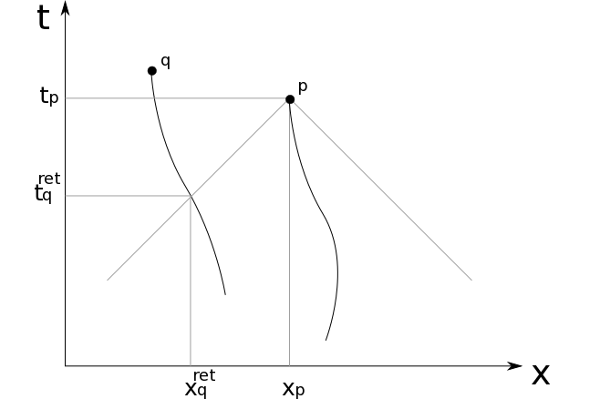
Figure 1: Intersection of the backward light cone of the observation point at $x^{\mu}_{p}$ with the worldline $x^{\mu}_{q}(\tau)$ of particle $q$ in Minkowski space.

9 Conclusions

Starting from the field equations of electrodynamics equations of motion for scalar quasi-electrons and positrons have been derived. Together with their radiation fields they form a set of MD equations with self-force effects. The derivation of the latter makes use of the energy-momentum tensors of the matter and radiation fields. In the paper the LAD terms for radiation reaction have been motivated.