Accurate Interatomic Force Fields via Machine Learning with Covariant Kernels

Abstract

We present a novel scheme to accurately predict atomic forces as vector quantities, rather than sets of scalar components, by Gaussian Process (GP) Regression. This is based on matrix-valued kernel functions, on which we impose the requirements that the predicted force rotates with the target configuration and is independent of any rotations applied to the configuration database entries. We show that such covariant GP kernels can be obtained by integration over the elements of the rotation group $SO(d)$ for the relevant dimensionality $d$. Remarkably, in specific cases the integration can be carried out analytically and yields a conservative force field that can be recast into a pair interaction form. Finally, we show that restricting the integration to a summation over the elements of a finite point group relevant to the target system is sufficient to recover an accurate GP. The accuracy of our kernels in predicting quantum-mechanical forces in real materials is investigated by tests on pure and defective Ni, Fe and Si crystalline systems.

I Introduction

Recent decades have witnessed an exponential growth of computer processing power (“Moore’s Law” Moore:1998gt ) and an equally fast progress of storage technology (“Kryder’s Law” Walter:2005be ; Grochowski:2003gg ). Atomistic modelling methods based on computation and data-intensive quantum mechanical methods, such as Density Functional Theory (DFT) Hartree:2008fd ; Fock:1930dx ; Slater:1951en , have correspondingly evolved in both feasibility and scope. Moreover, the possibility of retaining at low cost very large amounts of data generated by Quantum Mechanical (QM) codes has prompted novel efforts to make the data openly accessible Untitled:Bxh2cefs .

The information contained in the data can thus be harnessed and re-used indefinitely, in various ways. High throughput techniques are routinely used to identify new correlations between physical properties, with the aim of designing new high-performance materials Ghiringhelli:2015kr ; Pilania:2013di ; Kim:2016ev . Inference techniques can meanwhile also be used as a boost or substitute for QM techniques. This typically involves predicting a physical property for a new system configuration, on the basis of its values for an existing database of configurations. If the database is sufficiently large and representative, the new property values can be quickly inferred, rather than calculated anew by expensive QM procedures, with controllable accuracy.

Machine Learning techniques have been successfully used to predict properties as diverse as atomisation energies Rupp:2012kxa , density functionals Snyder:2012da , Green’s functions Arsenault:2014ema , electronic transport coefficients LopezBezanilla:2014iq , potential energy surfaces Bartok:2010fj ; Behler:2007fe ; Shapeev:2016kn and free energy landscapes Stecher:2014gi . The high configuration space complexity of real chemical systems has also inspired “learning” molecular dynamics schemes that never assume database completeness, but rather combine inference with on-the-fly QM calculations (learning on-the-fly, LOTF) DeVita:1997fp ; Csanyi:2004dh ; Podryabinkin:2016ta carried out when inference is infeasible or not deemed sufficiently accurate.

A well established general concept within the Machine Learning community is that functional invariance properties under some known transformation can be used to improve prediction, whether this is carried out by e.g. Gaussian Process (GP) regression Haasdonk:2007ff ; Williams:2006vz or neural networks Bishop:998831 . Exploiting in similar ways properties other than invariance has received more limited attention Krejnik:2012eo . In the same spirit, materials modellers have been successful in exploiting the invariance of energy under rotation or translation to improve the performance of energy prediction techniques Bartok:2010fj ; Behler:2007fe . In LOTF molecular dynamics applications the high-accuracy target and local interpolation character of force prediction makes it appealing to learn forces directly rather than learning a potential energy scalar field first and then deriving forces by differentiation. In previous works Li:2015eb ; Caccin:2015co ; Botu:2014kc this was accomplished by using GP regression to separately learn individual force components.

Here, we show how Vectorial Gaussian Process (VGP) Micchelli:2004uv ; Alvarez:2012ew regression provides a more natural framework for force learning, where the correct vector behaviour of forces under symmetry transformations can be obtained by using a new family of vector kernels of covariant nature. These kernels prove particularly efficient at exploiting the information contained in QM force databases, however constructed, together with any prior knowledge of the symmetry properties of the physical system under investigation. The next section provides a brief overview of the notion of a VGP, where we pay particular attention to the problem of force learning. Then we define a covariant kernel, explain its symmetry properties and give a general recipe to generate such kernels. The procedure is best exemplified by looking at one and two dimensional systems, where the relevant symmetry force transformation groups are $D_{1}$ and $O(2)$. Finally we address the full three dimensional case, where covariant kernels are tested by examining their performance in learning QM forces in realistic physical systems.

II Vectorial Gaussian Process Regression

We wish to model by a VGP the force $\mathbf{f}$ acting on an atom whose chemical environment is in a configuration $\mathbf{\rho}$ that encodes the positions of all neighbours of the atom, up to a suitable cutoff radius, in an arbitrary Cartesian reference frame. In the absence of long range ionic interactions, the existence of such a local map is guaranteed for all finite-temperature systems by the "nearsightedness" principle of electronic matter Kohn:1996hn ; Prodan:2005eu .

In a Bayesian setting, before any data is considered, $\mathbf{\mathbf{f}}$ is treated as a Gaussian Process, i.e., it is assumed that for any finite set of configurations $\{\rho_{i,\,}i=1,\dots N\}$ the values $\mathbf{f}(\rho_{i})$ taken by the vector function $\mathbf{f}$ are well described by a multivariate Gaussian distribution Williams:2006vz . We write:

$$\mathbf{f}(\rho)\sim\mathcal{GP}(\mathbf{m}(\rho),\mathbf{K}(\rho,\rho^{\prime}))$$ (1)

where $\mathbf{m}(\rho)$ is a vector-valued mean function and $\mathbf{K}(\rho,\rho^{\prime})$ is a matrix-valued kernel function. Before any data is considered, $\mathbf{m}$ is usually assumed to be zero as all prior information on $\mathbf{f}$ is encoded into the kernel function $\mathbf{K}(\rho,\rho^{\prime})$. The latter represents the correlation of the vectors $\mathbf{f}(\rho)$ and $\mathbf{f}(\rho^{\prime})$ as a function of the two configurations (“input space points”) $\rho$ and $\rho^{\prime}$:

$$\mathbf{K}(\rho,\rho^{\prime})=\langle\mathbf{f}(\rho)\mathbf{f}^{{\rm T}}(\rho^{\prime})\rangle,$$ (2)

where angular brackets here signify the expected value over the multivariate Gaussian distribution. Any kernel $\mathbf{K}$ consistent with this definition must be a positive semi-definite matrix function, since for any collection of vectors $\{\mathbf{v}_{i}\}$

$$\sum_{ij}\mathbf{v}_{i}^{{\rm T}}\mathbf{K}(\rho_{i},\rho_{j})\mathbf{v}_{j}=\langle(\sum_{i}\mathbf{v}_{i}^{{\rm T}}\mathbf{f}(\rho_{i}))^{2}\rangle\geq 0.$$ (3)

To train the prediction model we need to access a database of atomic configurations and reference forces $\mathcal{D}=\{(\rho,\mathbf{f}^{r})_{i},\,i=1,\dots,N\}$. Using Bayes’ theorem Bayes:1763ug the distribution (1) is modified to take the data $\mathcal{D}$ into account Williams:2006vz . If the likelihood function Bishop:998831 is also Gaussian (which effectively assumes that the observed forces $\mathbf{f}_{i}^{r}$ are the true forces subject to Gaussian noise of variance $\sigma_{n}^{2}$) then the resulting posterior distribution $\mathbf{f}(\rho\mid\mathcal{D})$, conditional on the data, will also be a Gaussian process

$$\mathbf{f}(\rho\mid\mathcal{D})\sim\mathcal{GP}(\mathbf{\hat{f}}(\rho\mid\mathcal{D}),\mathbf{\hat{C}}(\rho,\rho^{\prime})).$$ (4)

The mean function of the posterior distribution, $\hat{\mathbf{f}}(\rho\mid\mathcal{D})$, is at this point the best estimate for the true underlying function:

$$\hat{\mathbf{f}}(\rho\mid\mathcal{D})=\sum_{ij}^{N}\mathbf{K}(\rho,\rho_{i})[\mathbb{K}+\mathbb{I}\sigma_{n}^{2}]_{ij}^{-1}\mathbf{f}_{j}^{r}.$$ (5)

Here $\sigma_{n}^{2}$, formally the noise affecting the observed forces $\mathbf{f}^{r}$, serves in practice as a regulariser for the matrix inverse. In the following, blackboard bold characters such as $\mathbb{K}$ or $\mathbb{I}$ indicate $N\times N$ block matrices (for instance, the Gram matrix $\mathbb{K}$ is defined as $(\mathbb{K})_{ij}=\mathbf{{K}}(\rho_{i},\rho_{j})$). Similarly, we denote by $[\mathbb{K}+\mathbb{I}\sigma_{n}^{2}]_{ij}^{-1}$ the $ij$-block of the inverse matrix.

We next examine how to incorporate the vector behaviour of forces into the learning algorithm. The relevant symmetry transformations in the input space are: rigid translation of all atoms, permutation of atoms of the same chemical species, rotations and reflections of atomic configurations. Forces are invariant with respect to translations and atomic permutations, and covariant with respect to rotations and reflections. Assuming that the representation of the atomic configuration is local, i.e., the atom subject to the force $\mathbf{f}_{i}$ is at the origin of the reference frame used for $\rho_{i}$, translations are automatically taken into account. The remaining symmetries must be addressed in the construction of covariant kernels.

III Covariant Kernels

From now on we will define $\mathcal{S}$ to be any symmetry operator (rotation or reflection) acting on an atomistic configuration of a $d$-dimensional system. Rotations will be denoted by $\mathcal{R}$ and reflections by $\mathcal{Q}$.

We require two properties to apply to the predicted force $\hat{\mathbf{f}}(\rho\mid\mathcal{D})$, once configurations are transformed by an operator $\mathcal{S}$ (represented by a matrix $\mathbf{S}$):

Property 1

If the target configuration $\rho$ is transformed to $\mathcal{S}\rho$, the predicted force must transform accordingly:

$$\hat{\mathbf{f}}(\mathcal{S}\rho\mid\mathcal{D})=\mathbf{S}\hat{\mathbf{f}}(\rho\mid\mathcal{D}).$$ (6)

Property 2

The predicted force must not change if we arbitrarily transform the configurations in the database ($\mathcal{D}\rightarrow\tilde{\mathcal{D}}=\{(\mathcal{S}_{i}\rho_{i},\mathbf{S}_{i}\mathbf{f}_{i}^{r})\}$) with any chosen set of roto-reflections $\{\mathcal{S}_{i}\}$.

We next introduce a special class of kernel functions that automatically guarantees these two properties: a covariant kenrel has the defining property

$$\mathbf{K}(\mathcal{S}\rho,\mathcal{S}^{\prime}\rho^{\prime})=\mathbf{S}\mathbf{K}(\rho,\rho^{\prime})\mathbf{S}^{\prime{\rm T}}.$$ (7)

That a covariant kernel imposes Property 1 follows straightforwardly from Eq. (5):

$$\hat{\mathbf{f}}(\mathcal{S}\rho\mid\mathcal{D}) = \sum_{ij}^{N}\mathbf{K}(\mathcal{S}\rho,\rho_{i})[\mathbb{K}+\mathbb{I}\sigma_{n}^{2}]_{ij}^{-1}\mathbf{f}_{j}^{r}$$ (8)

$$= \sum_{ij}^{N}\mathbf{S}\mathbf{K}(\rho,\rho_{i})[\mathbb{K}+\mathbb{I}\sigma_{n}^{2}]_{ij}^{-1}\mathbf{f}_{j}^{r}$$

$$= \mathbf{S}\hat{\mathbf{f}}(\rho\mid\mathcal{D}).$$

To prove Property 2 we note that, if the kernel function is covariant, the transformed database $\tilde{\mathcal{D}}$ has Gram matrix $(\mathbb{\tilde{K}})_{ij}=\mathbf{K}(\mathcal{S}_{i}\rho_{i},\mathcal{S}_{j}\rho_{j})=\mathbf{S}_{i}\mathbf{K}(\rho_{i},\rho_{j})\mathbf{S}_{j}^{{\rm T}}$. If we define the block-diagonal matrix $\mathbb{S}_{ij}=\delta_{ij}\mathbf{S}_{i}$, this can be written in the simple block-matrix form $\mathbb{\tilde{K}}=\mathbb{\mathbb{S}K}\mathbb{S}^{{\rm T}}$. Using kernel covariance again to write $\mathbf{K}(\rho,\mathcal{S}_{i}\rho_{i})=\mathbf{K}(\rho,\rho_{i})\mathbb{S}_{ii}^{{\rm T}}$ the prediction associated with the transformed database $\tilde{\mathcal{D}}$ can be written as

$$\hat{\mathbf{f}}(\rho\mid\tilde{\mathcal{D}})=\sum_{ij}^{N}\mathbf{K}(\rho,\rho_{i})\mathbb{S}_{ii}^{{\rm T}}[\mathbb{S}\mathbb{K}\mathbb{S}^{{\rm T}}+\mathbb{I}\sigma_{n}^{2}]_{ij}^{-1}\mathbb{S}_{jj}\mathbf{f}_{j}^{r}.$$ (9)

By simple matrix manipulations it is now possible to show that in the above expression the symmetry transformations cancel out; indeed

$$\mathbb{S}^{{\rm T}}[\mathbb{S}\mathbb{K}\mathbb{S}^{{\rm T}}+\mathbb{I}\sigma_{n}^{2}]^{-1}\mathbb{S} = \mathbb{S}^{{\rm T}}[\mathbb{S}(\mathbb{K}+\mathbb{I}\sigma_{n}^{2})\mathbb{S}^{{\rm T}}]^{-1}\mathbb{S}$$ (10)

$$= \mathbb{S}^{{\rm T}}(\mathbb{S}^{{\rm T}})^{-1}[\mathbb{K}+\mathbb{I}\sigma_{n}^{2}]^{-1}\mathbb{S}^{{\rm-1}}\mathbb{S}$$

$$= [\mathbb{K}+\mathbb{I}\sigma_{n}^{2}]^{-1}$$

Equation (10) along with (9) implies $\hat{\mathbf{f}}(\rho\mid\mathcal{\tilde{{D}}})$ = $\hat{\mathbf{f}}(\rho\mid\mathcal{D})$, that is, Property 2. It is easy to check that standard kernels such as the squared exponential Bishop:998831 or the overlap integral of atomic configuration Ferre:2015dq do not possess the covariance property (7). Designing, entirely by feature engineering, a covariant kernel is in principle possible but can require complex tuning and is likely to be highly system dependent (see e.g. Li:2015eb ). We note that non covariant kernels can be used and avoid these difficulties, and some have been successfully implemented Botu:2014kc ; Botu:2015kb . This leaves space for improvement as prediction efficiency will generally be enhanced by increased exploitation of symmetry (see e.g., Figure 3 below for a simple test of this).

We next present a general method for transforming a standard matrix kernel into a covariant one, followed by numerical tests suggesting that the resulting kernel improves very significantly on the force-learning properties of the initial one, its error converging with just a fraction of the training data. This proceeds along the lines of previous techniques for generating scalar invariants, namely the transformation integration procedure developed in Haasdonk:2007ff and the Smooth Overlap of Atomic Orbitals (SOAP) representation for learning potential energy surfaces of atomic systems Bartok:2013cs ; Bartok:2015iw .

Given a group $\mathcal{S}$ and a base kernel $\mathbf{K}^{b}$, a covariant kernel $\mathbf{K}^{c}$ can be constructed by

$$\mathbf{K}^{c}(\rho,\rho^{\prime})=\int d\mathcal{S}_{1}d\mathcal{S}_{2}\mathbf{\,S}_{1}^{{\rm T}}\mathbf{K}^{b}(\mathcal{S}_{1}\rho,\mathcal{S}_{2}\rho^{\prime})\mathbf{S}_{2}$$ (11)

where $d\mathcal{S}$ is the normalised Haar measure for the symmetry group we are integrating over Mehta:1086514 .

The covariance of $\mathbf{K}^{c}$ as given by (11) is easily checked as

$$\mathbf{K}^{c}(\mathcal{S}\rho,\mathcal{S}^{\prime}\rho^{\prime}) = \int d\mathcal{S}_{1}d\mathcal{S}_{2}\mathbf{\,S}_{1}^{{\rm T}}\mathbf{K}^{b}(\mathcal{S}_{1}\mathcal{S}\rho,\mathcal{S}_{2}\mathcal{S}^{\prime}\rho^{\prime})\mathbf{S}_{2}$$ (12)

$$= \int d\tilde{\mathcal{S}}_{1}d\tilde{\mathcal{S}}_{2}\mathbf{\,S}\tilde{\mathbf{S}}_{1}^{{\rm T}}\mathbf{K}^{b}(\mathcal{\tilde{S}}_{1}\rho,\tilde{\mathcal{S}}_{2}\rho^{\prime})\tilde{\mathbf{S}}_{2}\mathbf{S}^{\prime{\rm T}}$$

$$= \mathbf{S}\mathbf{K}^{c}(\rho,\rho^{\prime})\mathbf{S}^{\prime{\rm T}}$$

where the second line follows from the substitutions $\tilde{\mathcal{S}}_{1}=\mathcal{S}_{1}\mathcal{S}$ and $\mathcal{\tilde{S}}_{2}=\mathcal{S}_{2}\mathcal{S}^{\prime}$. Note that these transformations have unit Jacobian because of the translational invariance (within the group) of any Haar measure Aubert:2003hs ; Mehta:1086514 .

It can be shown that the positive semi-definiteness of the base kernel is preserved under the operation (11) of covariant integration. In particular, a kernel is positive semi-definite if and only if it is a scalar product in some (possibly infinite dimensional) vector space Mercer:1909wb ; Williams:2006vz . Hence the base kernel can be written as $\mathbf{K}^{b}(\rho,\rho^{\prime})=\int d\alpha\boldsymbol{\,\phi}_{\alpha}(\rho)\boldsymbol{\phi}_{\alpha}^{{\rm T}}(\rho^{\prime}).$ It is then possible to show that its covariant counterpart $\mathbf{K}^{c}$ [Eq. (11)] will also be a scalar product in a new function space. Indeed

$$\mathbf{K}^{c}(\rho,\rho^{\prime}) = \int d\mathcal{S}_{1}d\mathcal{S}_{2}\mathbf{\,S}_{1}^{{\rm T}}\mbox{$\mathbf{K}$}^{b}(\mathcal{S}_{1}\rho,\mathcal{S}_{2}\rho^{\prime})\mathbf{S}_{2}$$ (13)

$$= \int d\alpha\,d\mathcal{S}_{1}d\mathcal{S}_{2}\,\mathbf{S}_{1}^{{\rm T}}\boldsymbol{\phi}_{\alpha}(\mathcal{S}_{1}\rho)\boldsymbol{\phi}_{\alpha}^{{\rm T}}(\mathcal{S}_{2}\rho^{\prime})\mathbf{S}_{2}$$

$$= \int d\alpha\boldsymbol{\,\psi}_{\alpha}(\rho)\boldsymbol{\psi}_{\alpha}^{{\rm T}}(\rho^{\prime})$$

where the new basis vectors were defined as $\boldsymbol{\psi}_{\alpha}(\rho)=\int d\mathcal{S}\,\mathbf{S}^{{\rm T}}\boldsymbol{\phi}_{\alpha}(\mathcal{S}\rho).$ Hence, $\mathbf{K}^{c}$ will also be positive definite.

The completely general procedure above can be cumbersome to apply in practice, because of the double integration over group elements in (11) and the dependence on the design of the base kernel matrix $\mathbf{K}^{b}$. As a simplification, we assume the base kernel to be of diagonal form; assuming equivalence of all space directions, we can then write

$$\mathbf{K}^{b}(\rho,\rho^{\prime})=\mathbf{\mathbf{I}}k^{b}(\rho,\rho^{\prime}).$$ (14)

where the scalar base kernel $k^{b}$ is independent on the reference frame in which the configurations are expressed. This requires that

$$k^{b}(\mathcal{S}\rho,\mathcal{S}\rho^{\prime})=k^{b}(\rho,\rho^{\prime}),$$ (15)

that is, scalar invariance of the base kernel (a property very commonly found in standard kernels). The double integration in (11) reduces at this point to a single one

$$\mathbf{K}^{c}(\rho,\rho^{\prime}) = \int d\mathcal{S}_{1}d\mathcal{S}_{2}\mathbf{\,S}_{1}^{{\rm T}}\mathbf{S}_{2}k^{b}(\mathcal{S}_{1}\rho,\mathcal{S}_{2}\rho^{\prime})$$ (16)

$$= \int d\mathcal{S}_{1}d\mathcal{S}_{2}\,\mathbf{S}_{1}^{{\rm T}}\mathbf{S}_{2}k^{b}(\rho,\mathcal{S}_{1}^{{\rm-1}}\mathcal{S}_{2}\rho^{\prime})$$

$$= \int d\mathcal{S}\,\mathbf{S}\,k^{b}(\rho,\mathcal{S}\rho^{\prime})$$

where the second line follows from property (15) and the third line is obtained by the substitution $\mathcal{S}=\mathcal{S}_{1}^{{\rm-1}}\mathcal{S}_{2}$.

In the next section we show that some base kernels allow analytical integration of (16). Here we note that incorporating our prior knowledge of the correct behaviour of forces in the kernel enables us to learn and predict forces associated with any configuration, regardless of its orientation. However, being able to do this for completely generic orientations is not always necessary. In many systems (e.g. crystalline solids where the orientation is known) all relevant configurations cluster around particular discrete symmetries. For these systems the relevant physics can be captured by restricting Eq. (11) to a discrete sum over the relevant group elements:

$$\mathbf{K}^{c}(\rho,\rho^{\prime})=\frac{1}{|G|}\sum_{\mathcal{G}\in G}\mathbf{G}k(\rho,\,\mathcal{G}\rho^{\prime}),$$ (17)

and since there are 48 distinct group elements at most (the order of the full $O_{48}$ group), the procedure remains computationally feasible. In the particular case of one-dimensional systems, where the only available symmetry operation other than the identity is the inversion, Eqs. (16) and (17) are formally equivalent.

IV Covariant Kernels from 1 to 3 dimensions

In the following we will assume that a single chemical species is present, so that permutation invariance will be simply enforced by representing configurations as linear combinations of $n$ Gaussian functions each centred on one atom, all having the same width $\sigma$, and suitably normalised depending on the dimension $d$ considered:

$$\rho(\mathbf{r},\{\mathbf{r}_{i}\})=\frac{1}{(2\pi\sigma^{2})^{d/2}}\sum_{i}^{n}\mathrm{e}^{-\frac{\|\mathbf{r}-\mathbf{r}_{i}\|^{2}}{2\sigma^{2}}}.$$ (18)

From (18), a linear base kernel $k_{L}^{b}$ can be defined as the overlap integral of two configurations Ferre:2015dq ; Bartok:2010fj

$$k_{L}^{b}(\rho,\rho^{\prime}) = \int d\mathbf{r}\,\rho(\mathbf{r},\{\mathbf{r}_{i}\})\rho^{\prime}(\mathbf{r},\{\mathbf{r}^{\prime}_{j}\})$$ (19)

$$= \frac{1}{(2\pi\sigma^{2})^{d}}\sum_{ij}^{nn^{\prime}}\int d\mathbf{r}\,\mathrm{e}^{-\frac{\|\mathbf{r}-\mathbf{r}_{i}\|^{2}}{2\sigma^{2}}}\mathrm{e}^{-\frac{\|\mathbf{r}-\mathbf{r}^{\prime}_{j}\|^{2}}{2\sigma^{2}}}$$

$$= \frac{1}{(2\sqrt{\pi\sigma^{2}})^{d}}\sum_{ij}\mathrm{e}^{-\frac{\|\mathbf{r}_{i}-\mathbf{r}^{\prime}_{j}\|^{2}}{4\sigma^{2}}}$$

where the integration yielding the third line is performed by standard completion of the square.

We can interpret the linear kernel $k_{L}^{b}$ in (19) as a scalar product in function space, so that $k_{L}^{b}(\rho,\rho)=\|\rho\|^{2}$ can be thought of as the squared norm of the $\rho$ configuration function. A permutation invariant distance is also readily obtained as $d(\rho,\rho^{\prime})=\|\rho-\rho^{\prime}\|$, which can be used within a squared exponential kernel to give

$$k_{SE}^{b}(\rho,\rho^{\prime}) = \mathrm{e}^{-\|\rho-\rho^{\prime}\|^{2}/2\theta}$$ (20)

$$= \mathrm{e}^{-(k_{L}^{b}(\rho,\rho)+k_{L}^{b}(\rho^{\prime},\rho^{\prime})-2k_{L}^{b}(\rho,\rho^{\prime}))/2\theta}.$$

The representation described above is by construction translation (and atomic permutation) invariant. We next address the transformations for which the atomic force is covariant, i.e., rotations and reflections, using the approach described in the previous section. Systems with dimensions $d=1,2,3$ are considered in the following three subsections. The first two provide a useful conceptual playground where the features of “covariant learning” can be more easily visualised. The third one benchmarks the method in real physical systems, simulated at the DFT level of accuracy.

IV.1 1D systems

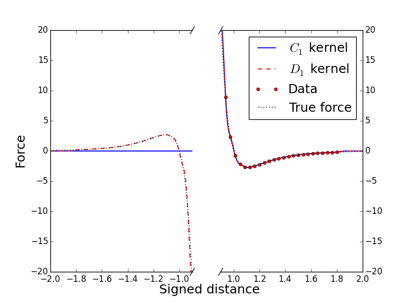
Figure 1: Lennard-Jones dimer force field, learned with data from one atom only. The base kernel ($C_{1}$) does not learn the symmetric counterpart (reaction force), while the covariant ($D_{1}$) does. The kernels are labelled by the symmetry group used to make them covariant; see main text for details.

A key feature of covariant kernels is the ability to enable “learning” of the entire set of configurations that are equivalent by symmetry to those actually provided in the database. For instance, the force acting on the (“central”) atom at the origin of configuration $\rho$ can be predicted even if only configurations $\rho^{\prime}$ of different symmetry are contained in the database. The only relevant symmetry transformation in 1D is the reflection $\mathcal{Q}$ of a configuration about its centre. In the simplest possible system, a dimer, this maps configurations where the central atom has a right neighbour (i.e. those for which the central atom is the left atom in the dimer) onto configurations where the central atom has a left neighbour. The covariant symmetrisation discussed in the previous section [Eq. (17)] takes the very simple form

$$k^{c}(\rho,\rho^{\prime})=\frac{1}{2}[k_{L}^{b}(\rho,\rho^{\prime})-k_{L}^{b}(\rho,\mathcal{Q}\rho^{\prime})].$$ (21)

Note that $k^{c}$ is identically zero for inversion-symmetric configurations $\rho$ or $\rho^{\prime}$ whose associated forces must vanish.

The force field associated with a 1D Lennard Jones dimer is plotted in Fig. 1 (dotted curve) as a function of a single signed number – the 1D vector going from the central atom to its neighbour. The figure also shows the predictions of the unsymmetrised base kernel using training data coming from configurations centred on the left atom only (solid blue curve). This closely reproduces the true LJ forces in the region where the data are available, and predicts the pure prior mean (i.e. zero) in the symmetry related region, i.e. the left half of the figure. Meanwhile, because of the covariant constraint (prior information) the GP based on the covariant kernel learns the left part of the field by just reflecting the right part appropriately.

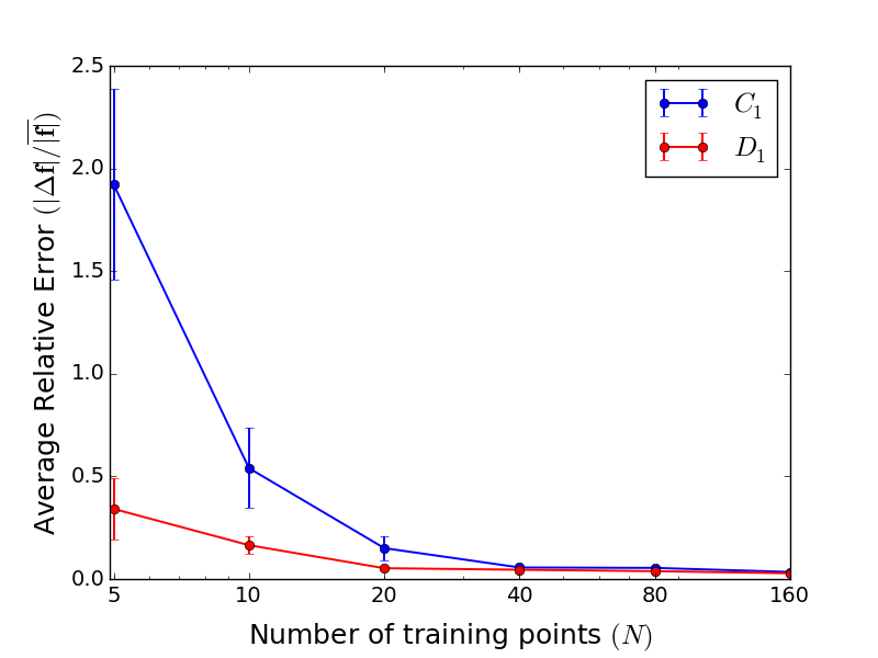
Figure 2: Learning Curves for a 1D chain of LJ atoms. The covariant kernel ($D_{1}$) learns twice as fast as the base one ($C_{1}$).

To further check the performance of the covariant kernel (21) we extended the comparison above to predicting the forces associated with a 1D Lennard Jones 50-atom chain system, in periodic boundary conditions. A database of training configurations and an independent test set of local configurations and forces were sampled from a constant temperature molecular dynamics simulation using a Langevin thermostat.

Before presenting the results, it is necessary to introduce some conventions that will apply throughout the rest of this work. As a measure of error between reference force $\mathbf{f}^{r}(\rho)$ and predicted force $\hat{\mathbf{f}}(\rho)$, we will take the absolute value of their vector difference $|\Delta\mathbf{f}|=|\mathbf{f}^{r}(\rho)-\hat{\mathbf{f}}(\rho)|$. Relative errors are obtained by dividing this absolute error by the time-ensemble average of the force modulus $\bar{|\mathbf{f}|}$. Average errors are found by randomly sampling $N$ training configurations and $1000$ test configurations. Repeating this operation provides the standard deviation and hence the error bars on absolute and relative errors. We furthermore denote by $C_{n}$ the cyclic group of order $n$ and by $D_{n}$ the dihedral group (containing also reflections) of order $2n$ ($C_{1}$ hence indicates the trivial group).

With the above clarifications, we can proceed with the analysis of Figure 2, which reports the average relative force error made by the GP regression on the test set as a function of training set size. It is immediately apparent that the covariant kernel performance is comparable to that of the base kernel with double the number of data points for training. We will observe the same effect also in two and three dimensions: symmetrising over a relevant finite group of order $|G|$ gives rise to an error drop approximately equivalent to a $|G|$-fold increase in the number of training points. Since the computational complexity of training a GP is $\mathcal{O}(N^{3})$, this can obviously lead to significant computer time savings.

IV.2 2D systems

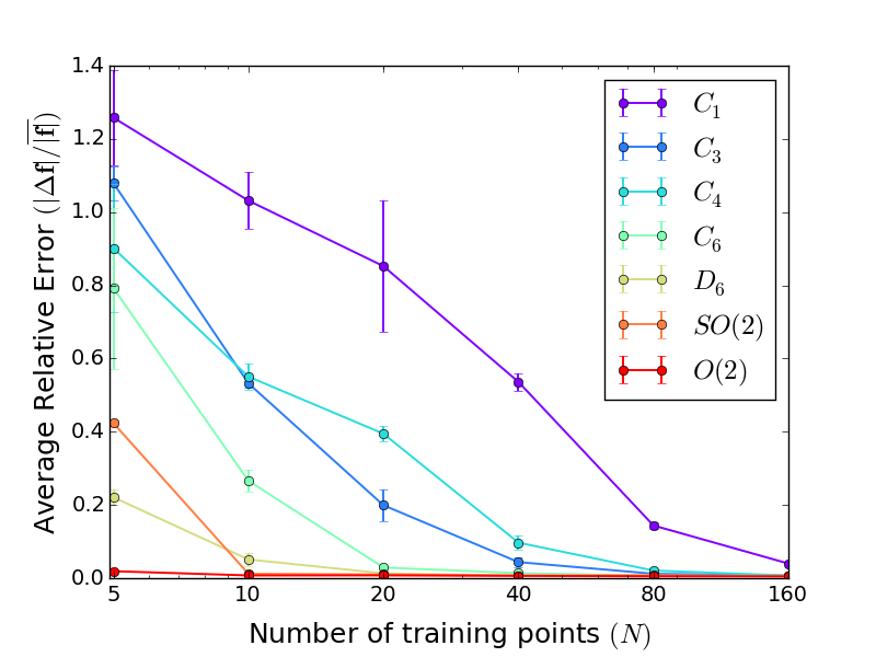
Figure 3: Learning curves for 2D triangular grid of LJ atoms. The larger the symmetry group used to construct the kernel, the faster the learning, provided that the lattice symmetry is captured.

In two dimensions all rotations and reflections, as well as any combination of these, are elements of $O(2)$. Moreover, the $O(2)$ group can be represented by the following set of matrices $O(2)=\{\mathbf{R}(\theta),\,\theta\in(0,2\pi]\}\cup\{\mathbf{R}(\theta)\mathbf{Q},\,\theta\in(0,2\pi]\}$ where $\mathbf{R}(\theta)=\begin{pmatrix}\cos(\theta)&\sin(\theta)\\ -\sin(\theta)&\cos(\theta)\end{pmatrix}$ and $\mathbf{Q}$ is any $2\times 2$ reflection matrix.

This makes the covariant integration (16) over $O(2)$ trivial once the matrix elements resulting from the integration over $SO(2)$ have been calculated. We next carry out the integration for the linear base kernel of Eq. (19). This can be expressed as a sum of pair contributions, where the first atom in each pair belongs to $\rho$ and the second to $\rho^{\prime}$ :

$$\mathbf{K}_{SO(2)}^{c}(\rho,\rho^{\prime})=\frac{1}{L}\sum_{ij}^{nn^{\prime}}\int_{SO(2)}d\mathcal{R}\,\mathbf{R}\,\mathrm{e}^{-\frac{\|\mathbf{r}_{i}-\mathbf{R}\mathbf{r}^{\prime}_{j}\|^{2}}{4\sigma^{2}}}.$$ (22)

Consistent with Eq. (16), only one atom of the pair is rotated during the integration, with $L$ being the normalisation factor [cf. Eq. (19)]. The pairwise integrals in (22) are calculated in two steps. We first define $\mathbf{R}_{ij}$ to be the rotation matrix which aligns $\mathbf{r}_{j}^{\prime}$ onto $\mathbf{r}_{i}$, and then perform the change of variable $\tilde{\mathbf{R}}=\mathbf{R}\mathbf{R}_{ij}^{{\rm T}}$ (and analogously $\mathcal{\tilde{R}=\mathcal{R}\mathcal{R}}_{ij}^{-1}$) yielding

$$\mathbf{K}_{SO(2)}^{c}(\rho,\rho^{\prime})=\frac{1}{L}\sum_{ij}\left(\int_{SO(2)}d\mathcal{\tilde{R}}\,\tilde{\mathbf{R}}\,\mathrm{e}^{-\frac{\|\mathbf{r}_{i}-\tilde{\mathbf{R}}\mathbf{R}_{ij}\mathbf{r}^{\prime}_{j}\|^{2}}{4\sigma^{2}}}\right)\mathbf{R}_{ij}.$$ (23)

Since the two vectors $\mathbf{r}_{i}$ and $\mathbf{R}_{ij}\mathbf{r}_{j}^{\prime}$ are now aligned, the integral in Eq. (23) can only depend on the two moduli $r_{i}$ and $r_{j}^{\prime}$ . The final result takes a very simple analytic form (cf. Supplemental Material):

$$\mathbf{K}_{SO(2)}^{c}(\rho,\rho^{\prime})=\frac{1}{L}\sum_{ij}\mathrm{e}^{-\frac{r_{i}^{2}+r_{j}^{\prime 2}}{4\sigma^{2}}}I_{1}\left(\frac{r_{i}r_{j}^{\prime}}{2\sigma^{2}}\right)\mathbf{R}_{ij}$$ (24)

where $I_{1}(\cdot)$ is a modified Bessel function of the first kind. The kernel in (24) is rotation-covariant by construction as can be seen immediately by comparison with Eq. (7).

By exploiting the internal structure of the orthogonal group discussed above, it is straightforward to show that the roto-reflection covariant kernel is given by

$$\mathbf{K}_{O(2)}^{c}(\rho,\rho^{\prime})=\frac{1}{2}\left(\mathbf{K}_{SO(2)}^{c}(\rho,\rho^{\prime})+\mathbf{K}_{SO(2)}^{c}(\rho,\mathcal{Q}\rho^{\prime})\mathbf{Q}\right),$$ (25)

which is the two-dimensional analog of Eq. (21). Interestingly, the resulting kernel can be also cast in the more intuitive form

$$\mathbf{K}_{O(2)}^{c}(\rho,\rho^{\prime})=\frac{1}{L}\sum_{ij}\mathrm{e}^{-\frac{r_{i}^{2}+r_{j}^{\prime 2}}{4\sigma^{2}}}I_{1}\left(\frac{r_{i}r_{j}^{\prime}}{2\sigma^{2}}\right)\hat{\mathbf{r}}_{i}\hat{\mathbf{r}}_{j}^{\prime{\rm T}},$$ (26)

where the hat denotes a normalised vector. Equation (26) implies that the predicted force on an atom at the centre of a configuration $\rho$ will be a sum of pairwise forces oriented along the directions $\hat{\mathbf{r}}_{i}$ connecting the central atom with each of its neighbours (while each neighbour will experience a corresponding reaction force). The modulus of these forces will be a function of the interatomic distance completely determined by the training database, whose integral can be thought of as a pairwise energy potential. Clearly then, the resulting force field will be conservative: for any fixed database, the forces predicted by GP inference using this kernel will do zero work if integrated along any closed trajectory loop in configuration space.

To test the relative performance of the learning models discussed above, we constructed training and test databases for a two-dimensional triangular lattice, sampled from a constant temperature molecular dynamics simulation of a 48-particle system interacting via standard Lennard-Jones forces, once more using periodic boundary conditions and a Langevin thermostat. As the chosen lattice has three-fold and six-fold symmetry, we can also examine the performance of covariant kernels that obey the two properties described above restricted to appropriate finite groups; these kernels are constructed as in Eq. (17). In this way we can monitor how imposing a progressively higher degree of symmetry on the kernel changes the rate at which forces in this system can be learned.

Our results are reported in Fig. 3. As anticipated, we find that the discrete covariant summation over the elements of a group $G$ is approximately equivalent to a $|G|$-fold increase in the number of data points. This can be seen e.g. from the results for the $C_{3}$ kernel (3-fold rotations) and the $C_{6}$ kernel (6-fold rotations), by comparing the error incurred in the two cases using $20$ and $10$ datapoints, respectively. More generally, we observe that the larger the group, the faster the learning. Note, however, that for the covariant summation (17) to extract content from the database that is actually useful for predicting forces in the test configurations at hand, the group used must describe a true underlying point symmetry of the system. Hence, for instance, the $C_{4}$ kernel gives rise to much slower learning than the $C_{3}$ kernel for the 2D triangular lattice examined. Consistently, for this lattice the full point group $D_{6}$ performs almost as well as the continuous symmetry kernels, suggesting that not much more is to be gained once the full (finite-group) symmetry of a system has been captured. This finding enables accurate force prediction in crystalline system when base kernels are used for which the covariant integration cannot be performed analytically, because the summation over a discrete symmetry group is available as a viable alternative.

IV.3 3D systems

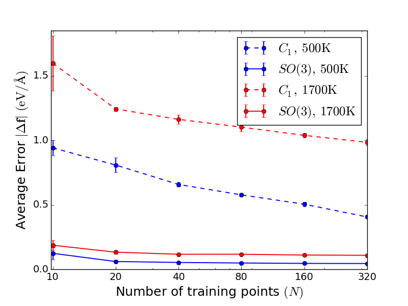
Figure 4: Learning Curves for crystalline nickel at two target temperatures. The $SO(3)$ covariant kernel (full lines) outperforms the base one (dashed lines).

We next benchmark the accuracy of our kernels in predicting DFT forces in three-dimensional bulk metal systems. As in the 2D case, starting from the linear base kernel we proceed to carry out the covariant integration analytically. After expressing the integration as a sum of pairwise integrals, the position vectors $\mathbf{r}_{i}$ and $\mathbf{\mathbf{r}}_{j}^{\prime}$ of two atoms in each pair are aligned onto each other. A convenient way to achieve this is by making both vectors parallel to the $z$-axis with appropriate rotations $\mathbf{R}_{i}^{z}$ and $\mathbf{R}_{j}^{z}$. As before, the covariant integration will yield a matrix whose elements are scalar functions of the radii $r_{i}$ and $r_{j}^{\prime}$ only. The integration can be carried out analytically over the standard three Euler angle variables (cf. Supplemental Material for further details). Due to the $z$-axis orientation, the kernel matrix elements turn out to be all zero except for the $zz$ one. The result reads

$$\mathbf{K}_{SO(3)}^{c}(\rho,\rho^{\prime}) = \frac{1}{L}\sum_{ij}\mathbf{R}_{i}^{z{\rm T}}\begin{pmatrix}0&0&0\\ 0&0&0\\ 0&0&\phi(r_{i},r_{j}^{\prime})\end{pmatrix}\mathbf{R}_{j}^{z},$$

$$\phi(r_{i},r_{j}) = \frac{\mathrm{e}^{-\alpha_{ij}}}{\gamma_{ij}^{2}}(\gamma_{ij}\cosh\gamma_{ij}-\sinh\gamma_{ij}),$$

$$\alpha_{ij} = \frac{r_{i}^{2}+r_{j}^{\prime 2}}{4\sigma^{2}},$$

$$\gamma_{ij} = \frac{r_{i}r_{j}^{\prime}}{2\sigma^{2}}.$$ (27)

As in the 2D case, this covariant kernel matrix can be rewritten in terms of the unit vectors $\hat{\mathbf{r}}_{i}$ and $\hat{\mathbf{r}}_{j}^{\prime}$ associated with the atoms of the configurations $\rho,\rho^{\prime}$ as

$$\mathbf{K}_{SO(3)}^{c}(\rho,\rho^{\prime})=\frac{1}{L}\sum_{ij}\phi(r_{i},r_{j}^{\prime})\hat{\mathbf{r}}_{i}\hat{\mathbf{r}}_{j}^{\prime{\rm T}},$$ (28)

making it apparent that the kernel models a pairwise conservative force field. However, while in 2D we needed to impose the full roto-reflection symmetry in order to obtain Eq. (26), rotations alone are sufficient to arrive at the fully covariant kernel in (28). This is a consequence of the fact that, in three dimensions, the covariant integral over rotations already imposes that the predicted force any atom will exert on any other is aligned along the vector connecting the pair: by symmetry there can be no preferred direction for an orthogonal force component after integrating over all rotations around the connecting vector, so that $\mathbf{K}_{O(3)}^{c}=\mathbf{K}_{SO(3)}^{c}$. This is not the case in two dimensions where covariant integration is over rotations around the $z$-axis orthogonal to all connecting vectors lying in the $xy$ plane, so that non-aligned predicted force components associated with a non-zero torque are not forbidden by symmetry in $\mathbf{K}_{SO(2)}^{c}$, and only the fully symmetrised kernel (25) will reduce to the pairwise form (26).

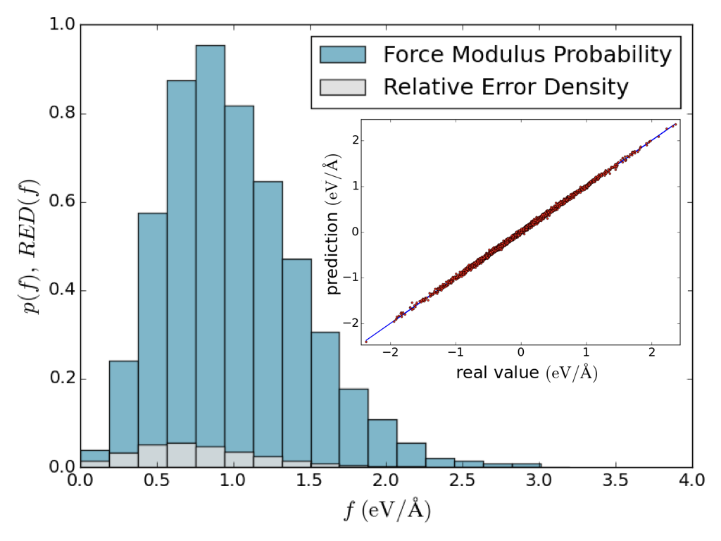
Figure 5: Density of relative error made by the GP algorithm ($N=320$) for bulk nickel at $500\rm{K}$. The inset shows the scatter plot of real vs. predicted cartesian components for the same data.

More generally we may conjecture that the rotationally covariant kernel $\mathbf{K}_{O(d)}^{c}$ derived from a linear base kernel predicts pairwise central forces, and hence is conservative, in any dimension $d$.

We note that energy conserving kernels have previously been obtained as double derivatives (Hessian matrices) of scalar energy kernels (as originally described in Refs. Narcowich:2007tl ; Macedo:2008vq and used for atomistic systems in Refs. in Bartok:2015iw to learn energies and more recently in Ref. Chmiela:2017ff to learn forces). However, no closed-form expressions exist for the energy kernels that would yield our $O(d)$ energy conserving kernels through this route, since the required double integration of the kernels (21), (26), (28) cannot be carried out analytically.

To test our models, we performed DFT-accurate dynamical simulation with exchange and correlation energy modeled via the PBE/GGA approximation Perdew:1996iq . The systems considered were $4\times 4\times 4$ supercells of fcc nickel and bcc iron in periodic boundary conditions. A weakly coupled Langevin thermostat was used to control the temperature. We first examine bulk nickel at the target temperatures of $500{\rm K}$ and $1700{\rm K}$, i.e. for an intermediate temperature where anharmonic behaviour is already significant, and at a temperature close to the melting point where the strong thermal fluctuations make the system explore a more complex target configuration space. Figure 4 illustrates the performance of the kernel in Eq. (27) on this system.

The effect of adding symmetry information on the learning curve is very significant for both temperatures. In particular, the $SO(3)$ covariant kernel achieves a force error average lower than the $0.1\rm{eV}/\text{\AA}$ threshold using remarkably few training points: $10$ and $80$ for the lower and higher temperatures in this test, respectively. The errors of the most accurate models (achieved with a $N=320$ database) are particularly low: $0.0435(\pm 0.0006)\rm{eV}/\text{\AA}$ and $0.095(\pm 0.003)\rm{eV}/\text{\AA}$ respectively. Moreover, we note that the error on each force component (often reported in the literature, and different from the error on the full force vector used here) will be lower by a factor $\sqrt{3}$. This yields errors of $0.025\rm{eV}/\text{\AA}$ and $0.052\rm{eV}/\text{\AA}$ in the two cases, the former comparing well with the $0.09\rm{eV}/\text{\AA}$ value obtained by using a state of the art Embedded Atom Model (EAM) interatomic potential for nickel Mishin:2004bh ; Bianchini:2016jn .

Figure 5 allows one to assess the accuracy of the GP predictions in a complementary way: here we plot the probability distribution of the atomic forces as a function of the force modulus (blue histogram) and the associated relative error density (grey histogram). We define the latter as $RED(f)=\frac{|\Delta\mathbf{f}|}{f}p(f)$, which is normalised to $0.055$, reflecting the $5.5\%$ average relative error incurred by force prediction. The fact that $RED(f)$ is everywhere a small fraction of $p(f)$ demonstrates that a reasonable accuracy is achieved for the whole range of forces predicted.

The results presented so far indicate that fully exploiting symmetry significantly improves the accuracy of force prediction. Covariance is thus always used in the following analysis, where we compare the performance of different symmetry-aware kernels. We start by choosing iron systems for these tests as many properties of iron-based systems remain out of modelling reach. This is mostly due to technical limitations. On the one hand, full DFT calculations on large systems are too computationally expensive and even hybrid quantum-classical (“QM/MM”) simulations of iron systems are typically overwhelmingly costly, as they require large QM-zone buffered clusters to fully converge the forces Bianchini:cxBexsLf . On the other hand, in many situations even the best available, state of the art classical force fields may not guarantee accurate force prediction, as they may incur systematic errors Bianchini:cxBexsLf ; Bianchini:2016jn , or may be hard to extend to complex chemical compositions vonPezold:2011iz , so that a technique that can indefinitely re-use all computed QM forces via GP inference and produce results that are traceably aligned with DFT-accurate forces could be very useful Szlachta:2014jh ; Li:2015eb .

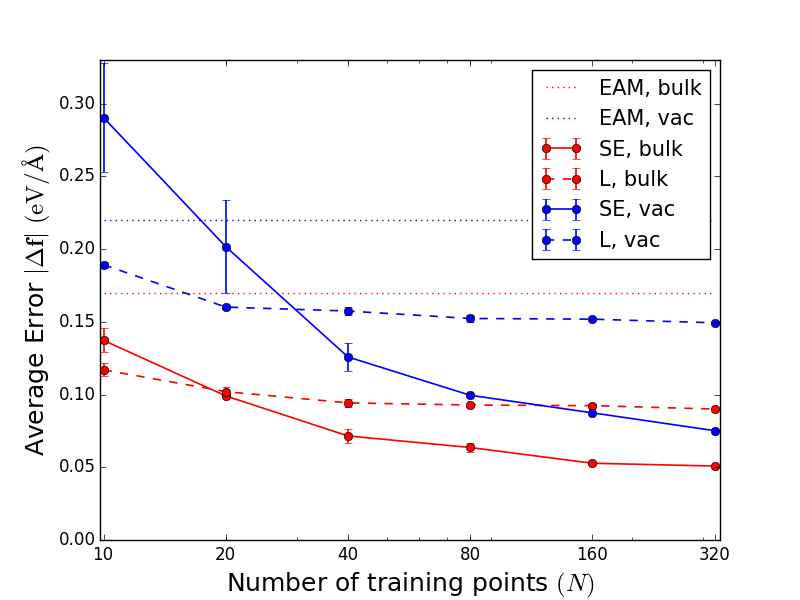
Figure 6: Learning curves associated with force prediction by the linear (L, dashed lines) and squared exponential (SE, solid lines) covariant kernels in bulk iron systems. Red and blue colours indicate undefected systems and model systems containing a vacancy, respectively.

We carried out constant temperature $(500{\rm K}$) molecular dynamics simulations of two bcc iron systems: a 64-atom crystalline system and a 63-atom system derived from this and containing a single vacancy. In the latter, only the atoms within the first two neighbour shells of the vacancy were used to test the algorithm, to better resolve the performance of our kernels in a defective system. Figure 6 shows the learning curves for the two symmetrised kernels: the linear kernel covariant over $O(3)$ and the squared exponential kernel (20) covariant over the full cubic point-group of the crystal. The figure also reports the performance of a high-quality EAM potential Mendelev:2003co . Both kernels perform better than the EAM potentials in this test. However, the error rate of the linear kernel (dashed lines) levels off to some constant non-zero value that might or might not be satisfactory (depending on the application), and will generally depend on the system being examined. In bulk iron the error floor value is about $0.09{\rm eV}/\text{\AA}$ while in the vicinity of a vacancy it is considerably higher ($0.15{\rm eV}/\text{\AA}$), suggesting that in spite of its many attractive properties (e.g. fast evaluation, fast convergence, energy conservation), the linear class of kernels of the form (28) is by no means complete, that is, it sometimes cannot capture and reproduce the entirety of the reference QM physical interaction. In many situations, kernels capable of reproducing higher order interactions could be needed to reach the target accuracy. This is exemplified by the much better performance of the squared exponential kernel (full lines in the figure), which yields higher accuracy, particularly for the more complex vacancy system (about $0.05{\rm eV}/\text{\AA}$ and $0.075{\rm eV}/\text{\AA}$ for atoms in the bulk and near the vacancy respectively). It is worth noting here that, in general, conserving energy exactly by construction provides no guarantee of higher force accuracy. For instance, in the case above, the squared exponential kernel delivers much more precise forces even though it conserves energy only approximately. As the approximation will in any case improve with the accuracy of the predicted forces, while no $SO(3)$-invariant energy conserving equivalent of this kernel has been proposed or appears viable, whether it is preferable to use this kernel or a less accurate but energy conserving alternative one, will generally depend on both the target system and the application at hand.

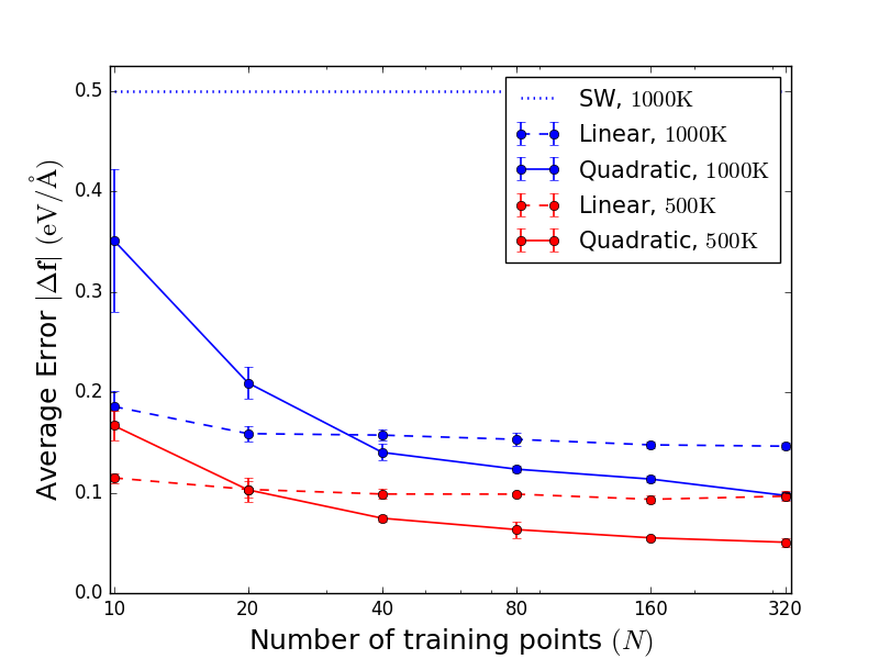
Figure 7: Learning curves obtained for crystalline silicon using the linear kernel (dashed lines) or the quadratic kernel (solid lines). Different colours indicate different temperatures.

For target systems with no clear point symmetry, a full covariant integration would always be desirable. This cannot be carried out analytically for the squared exponential kernel, where symmetrising by a discrete summation is the only option. However, interactions beyond pairwise can be still captured by the quadratic kernel obtained by taking the square of the linear kernel (19). In contrast to the squared exponential kernel, this is analytically tractable (for instance, an $SO(3)$-invariant scalar quadratic kernel was obtained in Bartok:2013cs ), and our analysis reveals that a matrix-valued quadratic kernel covariant over $O(3)$ can be derived analytically (details of the calculation are a subject for future work Glielmo:kZKvR16V ). The resulting model generates a roto-reflection symmetric three-body force field that can be expected to properly describe non close-packed bonding, such as found in covalent systems, for example.

Figure 7 illustrates the errors incurred by the linear and the quadratic kernel while attempting to reproduce the forces obtained during Langevin dynamics of a 64-atom crystalline silicon system using Density Functional Tight Binding (DFTB) Elstner:1998gh . Both linear and quadratic kernel are significantly more accurate than a classical Stillinger Weber (SW) potential Stillinger:1985zz fitted to reproduce the DFTB lattice parameter and bulk modulus Li:2015eb . Due to its more restricted associated function space, the linear kernel is the one that learns faster, and would be the more accurate if only very restricted databases had to be used. However, the quadratic kernel eventually performs much better than the (effective two-body) linear one for both of the temperatures, $500\rm{K}$ and $1000\rm{K}$, that we investigated in this covalent system. We obtain errors of $0.05{\rm eV}/\text{\AA}$ and $0.1{\rm eV}/\text{\AA}$ in the two cases, corresponding respectively to approximately $4\%$ and $6\%$ of the mean force. These are very close to the minimum baseline locality error Deringer:2017ea associated with the finite cutoff radius used for the Gaussian expansion in (18).

V Conclusion

In this work we presented a new method to learn quantum forces on local configurations. This method is based on a Vectorial Gaussian Process that encodes prior knowledge in a matrix valued kernel function. We showed how to include rotation and reflection symmetry of the force in the GP process via the notion and use of covariant kernels. A general recipe was provided to impose this property on otherwise non-symmetric kernels. The essence of this recipe lies in a special integration step, which we call covariant integration, over the full roto-reflection group associated with the relevant number of system dimensions. This calculation can be performed analytically starting from a linear base kernel, and the resulting $O(d)$ covariant kernels can be shown to generate conservative force fields.

We furthermore tested covariant kernels on standard physical systems in one, two and three dimensions. The one- and two-dimensional scenarios served as playgrounds to better understand and illustrate the essential features of such learning. The 3D systems allowed some practical benchmarking of the methodology in real systems. In agreement with what physical intuition would suggest, we consistently found that incorporating symmetry gives rise to more efficient learning. In particular, if both database and target configurations belong to a system with a definite underlying symmetry, restricting kernel covariance to the corresponding finite symmetry group will deliver the full speed-up of error convergence with respect to database size. At the same time this approach lifts the requirement of analytical integrability over the full $SO(d)$ manifold, as the restricted integration becomes a simple discrete sum over the relevant finite set of group elements. Testing on nickel, silicon and iron (the latter both pure and defective) reveals that the present recipes can improve significantly on available classical potentials. In general, non-linear kernels may be needed for accurate force predictions in the presence of complicated interactions, e.g. in the study of plasticity or embrittlement/fracture behaviour of covalent or metallic systems. In particular, a quadratic base kernel yields a fully $O(3)$ covariant effective three-body force field, and our tests suggest that this can be used successfully to improve the accuracy of force prediction in covalent materials. Current work is focussing on amorphous Si systems, where the lack of a clear point symmetry makes the full $O(3)$ covariance strictly necessary.

Our results reveal that force covariance is achievable without imposing energy conservation to the kernel form. While both are desirable properties, we find that lifting the exact energy conservation constraint can sometimes yield higher force accuracy. For instance, no invariant local energy based kernel has been proposed for the squared exponential ("universal approximator") kernel, since the analytic integration over $SO(3)$ is not viable. However, we find that covariance limited to the $O_{48}$ point group is very effective for force predictions in crystalline Fe systems using this kernel (see Fig. 6).

In general, while predicting forces with high accuracy is the main motivation for machine learning-based work in this field, the best compromise between accuracy, energy conservation and covariance will depend on the specific target application. For instance, kernels built from a covariant integration (or summation) that do not conserve energy exactly should not be used as substitutes for conventional interatomic potentials to perform long NVE simulations, since they might in principle lead to non-negligible spurious energy drifts. This is not a problem in NVT simulations, where a thermostat exchanges energy with the system to achieve and conserve the target temperature, which will be able to compensate for any such drift if appropriately chosen Jones:2011fh . Furthermore, the same kernels will be particularly suited for schemes that are in all cases incompatible with strict energy conservation. These include the LOTF approach and any online learning scheme similarly involving a dynamically updated force model. They also include any highly accurate and transferable scheme based on a fixed, very large database where, to maximise efficiency, each force prediction only uses its corresponding most relevant database subset.

On the other hand, any usage style is possible for covariant kernels conserving energy exactly, such as the covariant linear kernels of Eqs. (21), (26), and (28). In fact, the conservative pairwise interaction forces generated by these covariant linear kernels can be easily integrated to provide effective “optimal” standard pairwise potentials for any application needing a total energy expression. We also note that while the pair interaction form would still ensure very fast evaluation of the predicted forces, its accuracy for complex systems could be improved by dropping the transferability requirement of a single pairwise function. In such a scheme, different system regions could conceivably be modelled by locally optimised forces/potentials, where the local tuning could be simply achieved by restricting the inference process to subsets of the database pertinent to each target region.

Supplemental Material

Covariant integration

The integral we wish to evaluate, repeated here for convenience, is

$$\mathbf{K}^{c}\ (\rho,\rho^{\prime}) = \frac{1}{L}\sum_{ij}\int d\mathcal{R}\,\mathbf{R}\mathrm{e}^{-(\mathbf{r}_{i}-\mathbf{Rr}_{j}^{\prime})^{2}/4\sigma^{2}}$$

$$= \frac{1}{L}\sum_{ij}I_{ij}.$$

First of all it is convenient to separate the radial part from the angular one as the first of these does not depend on rotations:

$$I_{ij} = \mathrm{e}^{-(r_{i}^{2}+r_{j}^{\prime 2})/4\sigma^{2}}\int d\mathcal{R}\,\mathbf{R}\,\mathrm{e}^{\mathbf{r}_{i}^{{\rm T}}\mathbf{Rr}_{j}^{\prime}/2\sigma^{2}}$$

$$= C_{ij}\int d\mathcal{R}\,\mathbf{R}\,\mathrm{e}^{\mathbf{r}_{i}^{{\rm T}}\mathbf{Rr}_{j}^{\prime}/2\sigma^{2}}.$$

2D systems

If we define $\mathbf{R}_{ij}$ to be the rotation matrix that brings the vector $\mathbf{r}_{j}^{\prime}$ onto $\mathbf{r}_{i}$, then we can perform the change of variable $\tilde{\mathbf{R}}=\mathbf{R}\mathbf{R}_{ij}^{{\rm T}}$

$$I_{ij} = C_{ij}\int d\mathcal{\tilde{R}}\,\tilde{\mathbf{R}}\,\mathrm{e}^{\mathbf{r}_{i}^{{\rm T}}\tilde{\mathbf{R}}\mathbf{R}_{ij}\mathbf{r}_{j}^{\prime}/2\sigma^{2}}\mathbf{R}_{ij}$$

$$= C_{ij}\int d\mathcal{\tilde{R}}\,\tilde{\mathbf{R}}\,\mathrm{e}^{\mathbf{r}_{i}^{{\rm T}}\tilde{\mathbf{R}}\tilde{\mathbf{r}}_{j}^{\prime}/2\sigma^{2}}\mathbf{R}_{ij}.$$

where the two vectors $\mathbf{r}_{i}$ and $\tilde{\mathbf{r}}_{j}$ are now aligned with each other. By parametrising all rotations by a single angle $\theta$ we can rewrite the above integration as

$$I_{ij} = C_{ij}\int_{0}^{2\pi}\frac{d\theta}{2\pi}\mathbf{\,R}(\theta)\mathrm{e}^{\mathbf{r}_{i}^{{\rm T}}\mathbf{R}(\theta)\tilde{\mathbf{r}}_{j}^{\prime}/2\sigma^{2}}\mathbf{R}_{ij}$$

$$= C_{ij}\left(\int_{0}^{2\pi}\frac{d\theta}{2\pi}\mathbf{\,R}(\theta)\mathrm{e}^{r_{i}r_{j}^{\prime}\cos\theta/2\sigma^{2}}\right)\mathbf{R}_{ij}.$$

The integral in brackets can now be given an analytic form. The rotation matrix $\mathbf{R}(\theta)$ is composed by $\cos\theta$ on the diagonal and $\{\sin\theta,-\sin\theta\}$ off the diagonal. Evaluating the above integration for such terms one finds that

$$\begin{cases}\int_{0}^{2\pi}\frac{d\theta}{2\pi}\cos\theta\,\mathrm{e}^{r_{i}r_{j}^{\prime}\cos\theta/2\sigma^{2}}&=I_{1}\left(\frac{r_{i}r_{j}^{\prime}}{2\sigma^{2}}\right)\\ \int_{0}^{2\pi}\frac{d\theta}{2\pi}\sin\theta\,\mathrm{e}^{r_{i}r_{j}^{\prime}\cos\theta/2\sigma^{2}}&=0\end{cases}$$

where $I_{1}(\cdot)$ is a modified Bessel function of the first kind. The second line follows because we are integrating an odd function over an even domain. The first line, on the other hand, results from a definition of modified Bessel functions of the first kind $I_{n}(z)$ for integer values of $n$ (Abramowitz:1972vl p. 376), i.e.

$$I_{n}(z)=\frac{1}{\pi}\int_{0}^{\pi}\mathrm{e}^{z\cos\theta}\cos(n\theta)d\theta.$$

Hence the final integral reads

$$I_{ij}=C_{ij}I_{1}\left(\frac{r_{i}r_{j}^{\prime}}{2\sigma^{2}}\right)\mathbf{R}_{ij}.$$

3D systems

In three dimensions, it is first of all convenient to cast the integral in the following form

$$I_{ij} = \int d\mathcal{R}\,\mathbf{R}\mathrm{e}^{-(\mathbf{r}_{i}-\mathbf{Rr}_{j}^{\prime})^{2}/4\sigma^{2}}$$

$$= \int d\mathcal{R}\,\mathbf{R}\,k^{p}(\mathbf{r}_{i},\mathbf{Rr}_{j}^{\prime}).$$

Now we can use the global invariance of the base pairwise kernels $k^{p}$, that is $k^{p}(\mathbf{r},\mathbf{r}^{\prime})=k^{p}(\mathbf{Rr},\mathbf{Rr}^{\prime})$, in order to align $\mathbf{r}_{i}$ onto the $z$-axis. We call the rotation that does so $\mathbf{R}_{i}^{z}$ and we have

$$I_{ij} = \int d\mathcal{R}\,\mathbf{R}\,k^{p}(\mathbf{R}_{i}^{z}\mathbf{r}_{i},\mathbf{R}_{i}^{z}\mathbf{Rr}_{j}^{\prime})$$

$$= \int d\mathcal{R}\,\mathbf{R}\,k^{p}(\tilde{\mathbf{r}}_{i},\mathbf{R}_{i}^{z}\mathbf{R}\mathbf{r}_{j}^{\prime}).$$

where we defined $\tilde{\mathbf{r}}_{i}=\mathbf{R}_{i}^{z}\mathbf{r}_{i}$. At this point we find the matrix $\mathbf{R}_{j}^{z}$ that brings also $\mathbf{r}_{j}$ parallel to the $z$-axis. We then insert it in front of $\mathbf{r}_{j}^{\prime}$ in the form of the identity $\mathbf{R}_{j}^{z{\rm T}}\mathbf{R}_{j}^{z}$:

$$I_{ij} = \int d\mathcal{R}\,\mathbf{R}\,k^{p}(\tilde{\mathbf{r}}_{i},\mathbf{R}_{i}^{z}\mathbf{R}\mathbf{R}_{j}^{z{\rm T}}\mathbf{R}_{j}^{z}\mathbf{r}_{j}^{\prime})$$

$$= \int d\mathcal{R}\,\mathbf{R}\,k^{p}(\tilde{\mathbf{r}}_{i},\mathbf{R}_{i}^{z}\mathbf{R}\mathbf{R}_{j}^{z{\rm T}}\tilde{\mathbf{r}}_{j}^{\prime})$$

where we again used the tilde notation to define the vector now aligned to the $z$-azis. Finally we perform the change of variables $\tilde{\mathbf{R}}=\mathbf{R}_{i}^{z}\mathbf{R}\mathbf{R}_{j}^{z{\rm T}}$ to obtain

$$I_{ij} = \mathbf{R}_{i}^{z{\rm T}}\int d\tilde{\mathcal{R}}\,\tilde{\mathbf{R}}\,k^{p}(\tilde{\mathbf{r}}_{i},\tilde{\mathbf{R}}\tilde{\mathbf{r}}_{j}^{\prime})\mathbf{R}_{j}^{z}$$

$$= \mathbf{R}_{i}^{z{\rm T}}\mathbf{R}_{ij}\mathbf{R}_{j}^{z}.$$

The central integral yielding $\mathbf{R}_{ij}$ remains to be performed. Its evaluation is considerably simpler than the original problem since now both vectors $\tilde{\mathbf{r}}_{i},\tilde{\mathbf{r}}_{j}^{\prime}$ are along the $z$-axis. Hence, by parametrising all rotations by Euler angles $\alpha,\beta,\gamma$ around the $z,y,z$ axes respectively, we find by geometric reasoning that the argument of the exponential has to be invariant upon rotations of angles $\alpha$ and $\gamma$ around the $z$-axis. In fact, we have that

$$\mathbf{R}_{ij}=C_{ij}\int\frac{d\alpha d\beta d\gamma\sin\beta}{8\pi^{2}}\mathbf{R}(\alpha,\beta,\gamma)\mathrm{e}^{r_{i}r_{j}^{\prime}\cos\beta/2\sigma^{2}}$$

where we made use of the normalised Haar measure $d\alpha d\beta d\gamma\sin\beta/8\pi^{3}$. The rotation matrix to be averaged reads

$$\mathbf{R}(\alpha,\beta,\gamma)=\begin{pmatrix}c_{\alpha}c_{\gamma}-c_{\beta}s_{\alpha}s_{\gamma}&-c_{\gamma}c_{\beta}s_{\alpha}-c_{\alpha}s_{\gamma}&s_{\alpha}s_{\beta}\\ c_{\gamma}s_{\alpha}+c_{\alpha}c_{\beta}s_{\gamma}&c_{\alpha}c_{\gamma}c_{\beta}-s_{\alpha}s_{\gamma}&-c_{\alpha}s_{\beta}\\ s_{\gamma}s_{\beta}&c_{\gamma}s_{\beta}&c_{\beta}\end{pmatrix}.$$

All the elements of the above matrix apart from the $zz$ element vanish since there is always either a sine or a cosine integrated over an entire period. By defining $\gamma_{ij}=r_{i}r_{j}^{\prime}/2\sigma^{2}$, the only non trivial integral reads

$$\int_{0}^{\pi}\frac{d\beta\sin\beta}{2}\cos\beta\mathrm{e}^{r_{i}r_{j}^{\prime}\cos\beta/2\sigma^{2}} = \int_{0}^{\pi}\frac{d\beta}{2}\frac{\sin(2\beta)}{2}\mathrm{e}^{\gamma_{ij}\cos\beta}$$

$$= \left[\frac{\mathrm{e}^{\gamma_{ij}\cos\beta}(1-\gamma_{ij}\cos\beta)}{2\gamma_{ij}^{2}}\right]_{0}^{\pi}$$

$$= \frac{\gamma_{ij}\cosh\gamma_{ij}-\sinh\gamma_{ij}}{\gamma_{ij}^{2}}.$$

References

- (1) G. E. Moore, “Cramming more components onto integrated circuits (Reprinted from Electronics, pg 114-117, April 19, 1965),” Proceedings of the Ieee, vol. 86, no. 1, pp. 82–85, Jan. 1998.
- (2) C. Walter, “Kryder’s Law,” Scientific American, vol. 293, no. 2, pp. 32–33, Aug. 2005.
- (3) E. Grochowski and R. D. Halem, “Technological impact of magnetic hard disk drives on storage systems,” IBM Systems Journal, vol. 42, no. 2, pp. 338–346, 2003.
- (4) D. R. Hartree, “The wave mechanics of an atom with a non-Coulomb central field. Part I. Theory and methods,” Mathematical Proceedings of the Cambridge Philosophical Society, 1928.
- (5) V. Fock, “Näherungsmethode zur Lösung des quantenmechanischen Mehrkörperproblems,” Zeitschrift für Physik, vol. 61, no. 1-2, pp. 126–148, 1930.
- (6) J. C. Slater, “A Simplification of the Hartree-Fock Method,” Physical review, vol. 81, no. 3, pp. 385–390, Feb. 1951.
- (7) Nomad Database, “http://nomad-repository.eu/cms/.”
- (8) L. M. Ghiringhelli, J. Vybiral, S. V. Levchenko, C. Draxl, and M. Scheffler, “Big Data of Materials Science: Critical Role of the Descriptor,” Physical Review Letters, vol. 114, no. 10, pp. 105 503–5, Mar. 2015.
- (9) G. Pilania, C. Wang, X. Jiang, S. Rajasekaran, and R. Ramprasad, “Accelerating materials property predictions using machine learning,” Scientific Reports, vol. 3, pp. 1–6, Sep. 2013.
- (10) C. Kim, G. Pilania, and R. Ramprasad, “From Organized High-Throughput Data to Phenomenological Theory using Machine Learning: The Example of Dielectric Breakdown,” Chemistry of Materials, vol. 28, no. 5, pp. 1304–1311, Mar. 2016.
- (11) M. Rupp, A. Tkatchenko, K. R. Müller, and O. A. von Lilienfeld, “Fast and Accurate Modeling of Molecular Atomization Energies with Machine Learning,” Physical Review Letters, vol. 108, no. 5, pp. 058 301–5, Jan. 2012.
- (12) J. C. Snyder, M. Rupp, K. Hansen, K. R. Müller, and K. Burke, “Finding Density Functionals with Machine Learning,” Physical Review Letters, vol. 108, no. 25, pp. 253 002–5, Jun. 2012.
- (13) L. F. Arsenault, A. Lopez-Bezanilla, O. A. von Lilienfeld, and A. J. Millis, “Machine learning for many-body physics: The case of the Anderson impurity model,” Physical Review B, vol. 90, no. 15, pp. 155 136–16, Oct. 2014.
- (14) A. Lopez-Bezanilla and O. A. von Lilienfeld, “Modeling electronic quantum transport with machine learning,” Physical Review B, vol. 89, no. 23, pp. 235 411–5, Jun. 2014.
- (15) A. P. Bartók, M. C. Payne, R. Kondor, and G. Csányi, “Gaussian Approximation Potentials: The Accuracy of Quantum Mechanics, without the Electrons,” Physical Review Letters, vol. 104, no. 13, pp. 136 403–4, Apr. 2010.
- (16) J. Behler and M. Parrinello, “Generalized Neural-Network Representation of High-Dimensional Potential-Energy Surfaces,” Physical Review Letters, vol. 98, no. 14, pp. 146 401–4, Apr. 2007.
- (17) A. V. Shapeev, “Moment Tensor Potentials: A Class of Systematically Improvable Interatomic Potentials,” Multiscale Modeling & Simulation, vol. 14, no. 3, pp. 1153–1173, Jan. 2016.
- (18) T. Stecher, N. Bernstein, and G. Csányi, “Free Energy Surface Reconstruction from Umbrella Samples Using Gaussian Process Regression,” Journal of Chemical Theory and Computation, vol. 10, no. 9, pp. 4079–4097, Sep. 2014.
- (19) A. De Vita and R. Car, “A Novel Scheme for Accurate Md Simulations of Large Systems,” MRS Proceedings, vol. 491, p. 473, Jan. 1997.
- (20) G. Csányi, T. Albaret, M. C. Payne, and A. De Vita, ““Learn on the Fly”: A Hybrid Classical and Quantum-Mechanical Molecular Dynamics Simulation,” Physical Review Letters, vol. 93, no. 17, pp. 175 503–4, Oct. 2004.
- (21) E. V. Podryabinkin and A. V. Shapeev, “Active learning of linear interatomic potentials,” Nov. 2016.
- (22) B. Haasdonk and H. Burkhardt, “Invariant kernel functions for pattern analysis and machine learning,” Machine Learning, vol. 68, no. 1, pp. 35–61, May 2007.
- (23) C. K. I. Williams and C. E. Rasmussen, “Gaussian processes for machine learning,” the MIT Press, 2006.
- (24) C. M. Bishop, Pattern Recognition and Machine Learning, ser. Information Science and Statistics. New York, NY: Springer, 2006.
- (25) M. Krejnik and A. Tyutin, “Reproducing Kernel Hilbert Spaces With Odd Kernels in Price Prediction,” IEEE Transactions on Neural Networks and Learning Systems, vol. 23, no. 10, pp. 1564–1573, Sep. 2012.
- (26) Z. Li, J. R. Kermode, and A. De Vita, “Molecular Dynamics with On-the-Fly Machine Learning of Quantum-Mechanical Forces,” Physical Review Letters, vol. 114, no. 9, pp. 096 405–5, Mar. 2015.
- (27) M. Caccin, Z. Li, J. R. Kermode, and A. De Vita, “A framework for machine-learning-augmented multiscale atomistic simulations on parallel supercomputers,” International Journal of Quantum Chemistry, Jun. 2015.
- (28) V. Botu and R. Ramprasad, “Adaptive machine learning framework to accelerate ab initiomolecular dynamics,” International Journal of Quantum Chemistry, Dec. 2014.
- (29) C. A. Micchelli and M. Pontil, “Kernels for multi-task learning,” in Advances in Neural Information Processing Systems. University at Albany State University of New York, Albany, United States, Jan. 2005.
- (30) M. A. Alvarez, L. Rosasco, and N. D. Lawrence, “Kernels for Vector-Valued Functions: A Review,” Foundations and Trends® in Machine Learning, vol. 4, no. 3, pp. 195–266, 2012.
- (31) W. Kohn, “Density Functional and Density Matrix Method Scaling Linearly with the Number of Atoms,” Physical Review Letters, vol. 76, no. 17, pp. 3168–3171, Apr. 1996.
- (32) E. Prodan and W. Kohn, “Nearsightedness of electronic matter,” Proceedings of the National Academy of Sciences, vol. 102, no. 33, pp. 11 635–11 638, Aug. 2005.
- (33) T. Bayes and M. Price, “An essay towards solving a problem in the doctrine of chances. by the late rev. mr. bayes, frs communicated by mr. price, in a letter to john canton, amfrs,” Philosophical Transactions (1683-1775), 1763.
- (34) G. Ferré, J. B. Maillet, and G. Stoltz, “Permutation-invariant distance between atomic configurations,” The Journal of Chemical Physics, vol. 143, no. 10, pp. 104 114–13, Sep. 2015.
- (35) V. Botu and R. Ramprasad, “Learning scheme to predict atomic forces and accelerate materials simulations,” Physical Review B, vol. 92, no. 9, pp. 094 306–5, Sep. 2015.
- (36) A. P. Bartók, R. Kondor, and G. Csányi, “On representing chemical environments,” Physical Review B, vol. 87, no. 18, pp. 184 115–16, May 2013.
- (37) A. P. Bartók and G. Csányi, “Gaussian approximation potentials: A brief tutorial introduction,” International Journal of Quantum Chemistry, vol. 115, no. 16, pp. 1051–1057, Apr. 2015.
- (38) M. L. Mehta, Random Matrices; 3rd ed., ser. Pure and applied mathematics series. San Diego, CA: Elsevier, 2004.
- (39) S. Aubert and C. S. Lam, “Invariant integration over the unitary group,” Journal of Mathematical Physics, vol. 44, no. 12, pp. 6112–21, 2003.
- (40) J. Mercer, “Functions of positive and negative type, and their connection with the theory of integral equations,” Proceedings of the Royal Society of London Series a-Containing Papers of a Mathematical and Physical Character, vol. 83, no. 559, pp. 69–70, Nov. 1909.
- (41) E. J. Fuselier Jr, “Refined error estimates for matrix-valued radial basis functions,” Ph.D. dissertation, Texas A&M University, May 2006.
- (42) I. Macêdo and R. Castro, Learning divergence-free and curl-free vector fields with matrix-valued kernels. Instituto Nacional de Matematica Pura e Aplicada, 2008.
- (43) S. Chmiela, A. Tkatchenko, H. E. Sauceda, I. Poltavsky, K. T. Schütt, and K. R. Müller, “Machine learning of accurate energy-conserving molecular force fields,” Science Advances, vol. 3, no. 5, p. e1603015, May 2017.
- (44) J. P. Perdew, K. Burke, and M. Ernzerhof, “Generalized Gradient Approximation Made Simple,” Physical Review Letters, vol. 77, no. 18, pp. 3865–3868, Oct. 1996.
- (45) Y. Mishin, “Atomistic modeling of the and ’-phases of the Ni–Al system,” Acta Materialia, vol. 52, no. 6, pp. 1451–1467, Apr. 2004.
- (46) F. Bianchini, J. R. Kermode, and A. De Vita, “Modelling defects in Ni–Al with EAM and DFT calculations,” Modelling and Simulation in Materials Science and Engineering, pp. 1–15, Apr. 2016.
- (47) F. Bianchini, A. Glielmo, J. R. Kermode, and A. De Vita, “In Preparation.”
- (48) J. von Pezold, L. Lymperakis, and J. Neugebeauer, “Hydrogen-enhanced local plasticity at dilute bulk H concentrations: The role of H-H interactions and the formation of local hydrides,” Acta Materialia, vol. 59, no. 8, pp. 2969–2980, May 2011.
- (49) W. J. Szlachta, A. P. Bartók, and G. Csányi, “Accuracy and transferability of Gaussian approximation potential models for tungsten,” Physical Review B, vol. 90, no. 10, pp. 104 108–6, Sep. 2014.
- (50) M. I. Mendelev, S. Han, D. J. Srolovitz, G. J. Ackland, D. Y. Sun, and M. Asta, “Development of new interatomic potentials appropriate for crystalline and liquid iron,” Philosophical Magazine, vol. 83, no. 35, pp. 3977–3994, Dec. 2003.
- (51) A. Glielmo, P. Sollich, and A. De Vita, “In Preparation.”
- (52) M. Elstner, D. Porezag, G. Jungnickel, J. Elsner, M. Haugk, T. Frauenheim, S. Suhai, and G. Seifert, “Self-consistent-charge density-functional tight-binding method for simulations of complex materials properties,” Physical Review B, vol. 58, no. 11, pp. 7260–7268, Sep. 1998.
- (53) F. H. Stillinger and T. A. Weber, “Computer simulation of local order in condensed phases of silicon,” Physical review, vol. B31, no. 8, pp. 5262–5271, 1985.
- (54) V. L. Deringer and G. Csányi, “Machine learning based interatomic potential for amorphous carbon,” Physical Review B, vol. 95, no. 9, p. 094203, Mar. 2017.
- (55) A. Jones and B. Leimkuhler, “Adaptive stochastic methods for sampling driven molecular systems,” The Journal of Chemical Physics, vol. 135, no. 8, pp. 084 125–12, 2011.
- (56) M. Abramowitz and I. A. Stegun, Handbook of mathematical functions with formulas, graphs, and mathematical tables. National Bureau of Standards: Applied Mathematics Series, 1972.