Effective sparse representation of X-Ray medical images

Abstract

Effective sparse representation of X-Ray medical images within the context of data reduction is considered. The proposed framework is shown to render an enormous reduction in the cardinality of the data set required to represent this class of images at very good quality. The particularity of the approach is that it can be implemented at very competitive processing time and low memory requirements.

I Introduction

Within the field of medical imaging for diagnosis, radiology generates huge volumes of data in the form of X-Ray images. Complying with archive provisions legislation, which may require to store the patient’s data for up to ten years, represents a demanding burden for hospitals and individual radiology practices. Additionally, the prompt distribution of remote radiology reporting is one of the challenges in teleradiology. These matters have led several radiological societies to recommend to use irreversible (or ‘lossy’) compression “in a manner that is visually imperceptible and/or without loss of diagnostic performance” [1].

At least for extensive use, the state of the art for lossy image compression are the JPEG and JPEG2000 standards. Both techniques belong to the category of transformation coding, because are based on a compression scheme that applies an invertible transformation as the first step in the process. JPEG uses the Discrete Cosine Transform (DCT) for that purpose and JPEG2000 the Discrete Wavelet Transform (DWT). Both transformations play the role of reducing the non-negligible points in the transformed domain. The transformation we adopt here for the same purpose is different in essence. Rather than transforming the data into an array of the same dimensionality to disregard some points there, we expand the representation domain and strive to achieve a highly sparse representation in the extended domain.

Apart from the perceived advantage of sparse representations for medical image processing and health informatics [2], the emerging theory of compressive sensing has introduced a strong reason to achieve sparsity. Within the compressive sensing structure the number of measurements needed for accurate representation of a signal informational content decreases if the sparsity of the representation improves [3, 4, 5].

This Communication presents a framework rendering high sparsity in the representation of X-Ray medical images. This is achieved by:

• Creating a large redundant ‘dictionary’ of suitable elements for the image decomposition.

• Applying effective strategies for selecting the particular elements which enable the sparse decomposition of a given image.

The goal is to achieve high sparsity, with high quality reconstruction, at competitive processing time. Comparison of the results arising from the proposed framework with those yielded by the traditional DCT or DWT approximations demonstrates a massive improvement in sparsity.

II Sparse Image Representation

Let’s start by introducing some notational convention: bold face lower and upper cases are used to represent one dimension (1D) and two dimension (2D) arrays, respectively. Standard mathematical fonts indicate component, e.g., $\mathbf{c}\in\mathbb{R}^{K}$ is an array of real components, $c(k),\,k=1,\ldots,K$, and $\mathbf{I}\in\mathbb{R}^{N_{x}\times N_{y}}$ an array of real elements, $I(i,j),\,i=1,\ldots,N_{x},\,i=1,\ldots,N_{y}$.

Restricting considerations to $l$-bit gray scale images, an image is represented by an array $\mathbf{I}\in\mathbb{R}^{N_{x}\times N_{y}}$ the elements of which, called intensity pixels, are given by integer numbers from 0 to $2^{l}$-$1$.

Within the adopted framework for representations using dictionaries an image $\mathbf{I}\in\mathbb{R}^{N_{x}\times N_{y}}$ is approximated by a linear decomposition of the form:

$$\mathbf{I}^{K}=\sum_{k=1}^{K}c(k)\mathbf{D}_{\ell_{k}},$$ (1)

where each $\mathbf{D}_{\ell_{k}}$ is an element of $\mathbb{R}^{N_{x}\times N_{y}}$ normalized to unity, called ‘atom’. The $K$-atoms in (1) are selected from a redundant set called a dictionary. A sparse approximation of $\mathbf{I}$ is an approximation of the form (1) such that the number of $K$-terms in the decomposition is significantly smaller than ${N=N_{x}N_{y}}$.

The problem of how to select from a given dictionary the sparsest possible representation of a signal is a NP-hard problem [6]. In practical applications one looks for ‘tractable sparse’ solutions. The mathematical methods which are used for this purpose are either based on the minimization of the $l_{1}$-norm [7, 8] or are greedy strategies which evolve by stepwise selection of atoms from the dictionary [9, 10, 11, 12, 13, 14, 15, 16, 17, 18, 19]. Greedy strategies are better suited for practical applications. In particular, in this work we consider algorithms which have been shown effective for approximating by partitioning [20, 21].

II-A Approximation of X-Ray medical images by partitioning

A characteristic of X-Ray medical images is that they can be best approximated in the wavelet domain. This entails to:

• Apply a wavelet transform to the image, i.e. to convert the intensity image $\mathbf{I}$ into a transformed array $\mathbf{U}$.

• Approximate the array $\mathbf{U}$.

• Invert the approximated array to recover the approximated intensity image.

The effectiveness of our proposal is based on (a) the suitability of the proposed dictionary and (b) the selection approach for approximating the transformed image by dividing it into small blocks $\mathbf{U}_{q},\,q=1,\ldots,Q$, which we refer to as a ‘partition’ of the array $\mathbf{U}$. Without loss of generality the blocks are assumed to be square of size $N_{b}\times N_{b}$. We restrict the dictionary to be separable, i.e., a $2$D dictionary $\mathcal{D}=\{\mathbf{D}_{i}\in\mathbb{R}^{N_{b}\times N_{b}}\}_{i=1}^{M}$, which is obtained as the tensor product $\mathcal{D}=\mathcal{D}^{x}\otimes\mathcal{D}^{y}$ of two 1D dictionaries $\mathcal{D}^{x}=\{\mathbf{d}^{x}_{n}\in\mathbb{R}^{N_{b}}\}_{n=1}^{M_{x}}$ and $\mathcal{D}^{y}=\{\mathbf{d}^{y}_{m}\in\mathbb{R}^{N_{b}}\}_{m=1}^{M_{y}}$, with $M_{x}M_{y}=M$. This represents an important saving in storage. Indeed, instead of having to store a $N_{b}^{2}\times M$ array, only two arrays of size $N_{b}\times M_{x}$ and $N_{b}\times M_{y}$ are to be stored. The reduction in computer memory requirements allows us to work with large dictionaries.

For $q=1,\ldots,Q$ every element $\mathbf{U}_{q}$ is approximated by an atomic decomposition as below:

$$\mathbf{U}_{q}^{k_{q}}=\sum_{n=1}^{k_{q}}c^{k_{q},q}(n)\mathbf{d}^{x}_{\ell^{x,q}_{n}}(\mathbf{d}^{y}_{\ell^{y_{,}q}_{n}})^{T},$$ (2)

where $(\mathbf{d}^{y}_{\ell^{y_{,}q}_{n}})^{T}$ indicates the transpose of $\mathbf{d}^{y}_{\ell^{y_{,}q}_{n}}\in\mathbb{R}^{N_{b}}$. The approximated array $\mathbf{U}^{K}$ is the result of assembling the approximated blocks, i.e., $\mathbf{U}^{K}=\hat{\operatorname{J}}_{q=1}^{Q}\mathbf{U}_{q}^{k_{q}}$, where $K=\sum_{q=1}^{Q}k_{q}$ and $\hat{\operatorname{J}}$ stands for the assembling operator, which reconstructs $\mathbf{U}^{K}\in\mathbb{R}^{N_{x}\times N_{y}}$ from the $Q$ disjoint blocks $\mathbf{U}_{q}^{k_{q}}\in\mathbb{R}^{N_{b}\times N_{b}}$.

The Sparsity Ratio (SR) arising from the approximation is defined as

$$\mathrm{SR}=\frac{NxNy}{K}=\frac{QN_{b}^{2}}{K}.$$

Our goal is to produce an effective high quality approximation with a high value of SR.

The quality of an image approximation is quantified by the Mean Structural SIMilarity (MSSIM) index [22, 23] and the classical Peak Signal-to-Noise Ratio (PSNR), calculated as

$$\mathrm{PSNR}=10\log_{10}\left(\frac{{(2^{l}-1)}^{2}}{\mathrm{MSE}}\right),\quad\mathrm{MSE}=\frac{\|\mathbf{I}-\mathbf{I}^{K}\|_{F}^{2}}{N_{x}N_{y}},$$

where $l$ is the number of bits used to represent the intensity of the pixels and $\|\cdot\|_{F}^{2}$ indicates the Frobenius norm induced by the Frobenius inner product, which for $\mathbf{G}_{1}\in\mathbb{R}^{N_{x}\times N_{y}}$ and $\mathbf{G}_{2}\in\mathbb{R}^{N_{x}\times N_{y}}$ is defined as

$$\left\langle\mathbf{G}_{1},\mathbf{G}_{2}\right\rangle_{F}=\sum_{i,j=1}^{N_{x},N_{y}}G_{1}(i,j)G_{2}\!(i,j).$$ (3)

Consequently,

$$\|\mathbf{G}_{1}\|_{F}^{2}=\sum_{i,j=1}^{N_{x},N_{y}}|G_{1}(i,j)|^{2}.$$ (4)

We aim at achieving high PSNR and MSSIM very close to one. The question then arises as to how to decide on the number of atoms, $k_{q}$, for approximating each block in the partition. One possibility is to approximate each block totally independently of the other blocks and up to a fixed tolerance error. This possibility has the advantage of enabling straightforward parallelization with multiprocessors. Nevertheless, linking the approximation of all the blocks through a global constraint on sparsity, or quality, usually amounts to improving sparsity results [20, 21].

II-B Effective greedy strategy for approximating by partitioning

The common step of the techniques we consider for constructing approximations of the form (2) is the stepwise selection of atoms for each block $q$. On setting $k_{q}=0$ and $\mathbf{R}_{q}^{0}=\mathbf{U}_{q}$ at iteration $k_{q}+1$ the algorithm selects the indices $\ell^{x,q}_{k_{q}+1}$ and $\ell^{y,q}_{k_{q}+1}$ as follows:

$$\ell^{x,q}_{k_{q}+1},\ell^{y,q}_{k_{q}+1}=\operatorname*{arg\,max}_{\begin{subarray}{c}n=1,\ldots,M_{x}\\ m=1,\ldots,M_{y}\end{subarray}}\left|\left\langle\mathbf{d}^{x}_{n},\mathbf{R}_{q}^{k_{q}}\mathbf{d}^{y}_{m}\right\rangle_{F}\right|,$$ (5)

where $\mathbf{R}_{q}^{k_{q}}=\mathbf{U}_{q}-\mathbf{U}_{q}^{k_{q}}$. For the calculation of $\mathbf{R}_{q}^{k_{q}}$ we find the coefficients in (2) through the orthogonal projection onto the subspace of selected atoms $\mathbb{V}_{k_{q}}={\mbox{\rm{span}}}\{\mathbf{d}^{x}_{\ell^{x,q}_{n}}(\mathbf{d}^{y}_{\ell^{y,q}_{n}})^{T}\}_{n=1}^{k_{q}}$, which is equivalent to the minimization of $\|\mathbf{R}_{q}^{k_{q}}\|_{F}$. For the effective calculation of the projections we may choose two different routes, depending on the size of the blocks in the partition.

• Adaptive biorthogonalization of the selected atoms $\mathbf{A}_{n}^{k_{q},q}=\mathbf{d}^{x}_{\ell^{x,q}_{n}}(\mathbf{d}^{y}_{\ell^{y,q}_{n}})^{T}\in\mathbb{R}^{N_{b}\times N_{b}},\,n=1,\ldots,k_{q}$. This route gives rise to what is known as the Orthogonal Matching Pursuit (OMP) approach [10]. Our implementation for separable dictionaries in 2D, termed OMP2D [24], involves the orthogonalization and re-orthogonalization of the selected atoms $\{\mathbf{A}_{n}^{k_{q},q}\}_{n=1}^{k_{q}}$, producing the orthogonal set $\{\mathbf{W}_{n}^{k_{q},q},\in\mathbb{R}^{N_{b}\times N_{b}}\}_{n=1}^{k_{q}}$, which allows for an effective calculation of the set $\{\mathbf{B}_{n}^{k_{q},q}\in\mathbb{R}^{N_{b}\times N_{b}}\}_{n=1}^{k_{q}}$. The elements of this set are biorthogonal to the atoms $\{\mathbf{A}_{n}^{k_{q},q}\}_{n=1}^{k_{q}}$ and are used to compute the coefficients in (2) as

  $$c_{n}^{k_{q},q}=\left\langle\mathbf{B}_{n}^{k_{q},q},\mathbf{I}_{q}\right\rangle_{F}.$$ (6)

• The Self Projected Matching Pursuit (SPMP) methodology [25], which uses the seminal Matching Pursuit (MP) method [9] as a mean to calculate orthogonal projections.

The implementation details of the above described OMP2D method are given in [24] (Appendix A). Such an implementation is very effective up to some block size. For larger blocks the use of the SPMP method, which in 2D for a separable dictionary is referred to as SPMP2D [25], is advised. Because it fully exploits the separability of dictionaries, the SPMP2D method is less demanding in terms of computer memory even though theoretically equivalent to OMP2D. Full details for its implementation are given in [25]. The algorithm to realize the self projection step is sketched below.

Suppose that for approximating the block $q$ the selection process has chosen $k_{q}$ linearly independent atoms labeled by the pair of indices $\{\ell^{x,q}_{n},\ell^{y,q}_{n}\}_{n=1}^{k_{q}}$ and let $\tilde{\mathbf{U}}_{q}^{k_{q}}$ be an atomic decomposition of the form

$$\tilde{\mathbf{U}}_{q}^{k_{q}}=\sum_{n=1}^{k_{q}}a^{q}(n)\mathbf{d}^{x}_{\ell^{x,q}_{n}}(\mathbf{d}^{y}_{\ell^{y_{,}q}_{n}})^{T},$$ (7)

where the coefficients $a^{q}(n),\,n=1,\ldots,k_{q}$ are arbitrary real numbers. Every array $\tilde{\mathbf{U}}_{q}\in\mathbb{R}^{N_{b}\times N_{b}}$ can be expressed as

$$\tilde{\mathbf{U}}_{q}=\tilde{\mathbf{U}}_{q}^{k_{q}}+\tilde{\mathbf{R}}.$$ (8)

For $\tilde{\mathbf{U}}_{q}^{k_{q}}$ to be the optimal representation of $\tilde{\mathbf{U}}_{q}$ in $\mathbb{V}_{k_{q}}={\mbox{\rm{span}}}\{\mathbf{d}^{x}_{\ell^{x,q}_{n}}(\mathbf{d}^{y}_{\ell^{y,q}_{n}})^{T}\}_{n=1}^{k_{q}}$, in the sense of minimizing the norm of the residue $\tilde{\mathbf{R}}$, it should be true that $\hat{P}_{\mathbb{V}_{k_{q}}}\tilde{\mathbf{R}}=0$. The SPMP2D method fulfills this property by approximating $\tilde{\mathbf{R}}$ in $\mathbb{V}_{k_{q}}$, via the MP method, and subtracting that component from $\tilde{\mathbf{R}}$. The next algorithm describes the procedure.

Iterative orthogonal projection

Given a set of previously selected atoms $\{\mathbf{d}^{x}_{\ell^{x,q}_{n}}(\mathbf{d}^{y}_{\ell^{y,q}_{n}})^{T}\}_{n=1}^{k_{q}}$ set $\mathbf{T}^{0}=0$, $\tilde{\mathbf{R}}^{0}=\tilde{\mathbf{R}}$, $j=1$ and at each iteration apply the steps below:

• Select the pair of indices such that

  $$\ell^{x,q}_{j},\ell^{y,q}_{j}=\operatorname*{arg\,max}_{\begin{subarray}{c}n=1,\ldots,k_{q}\\ m=1,\ldots,k_{q}\end{subarray}}\left|\left\langle\mathbf{d}^{x}_{\ell^{x,q}_{n}},\tilde{\mathbf{R}}^{j-1}\mathbf{d}^{y}_{\ell^{y,q}_{m}}\right\rangle_{F}\right|.$$ (9)

• Compute:

  $$t(j) = \left\langle\mathbf{d}^{x}_{\ell^{x,q}_{j}},\tilde{\mathbf{R}}^{j-1}\mathbf{d}^{y}_{\ell^{y,q}_{j}}\right\rangle,$$

  $$\tilde{\mathbf{R}}^{j} = \tilde{\mathbf{R}}^{j-1}-t(j)\mathbf{d}^{x}_{\ell^{x,q}_{j}}(\mathbf{d}^{y}_{\ell^{y,q}_{j}})^{T},$$

  $$\mathbf{T}^{j} = \mathbf{T}^{j-1}+t(j)\mathbf{d}^{x}_{\ell^{x,q}_{j}}(\mathbf{d}^{y}_{\ell^{y,q}_{j}})^{T}.$$

• Set $j\leftarrow j+1$ and repeat the process until for a given tolerance error $\epsilon$ the condition $\|\mathbf{T}^{j}-\mathbf{T}^{j-1}\|_{F}<\epsilon$ is reached.

The asymptotic exponential convergence of $\mathbf{T}^{j}\rightarrow\hat{P}_{\mathbb{V}_{k_{q}}}\tilde{\mathbf{R}}$ is proven in [26].

II-C Ranking blocks for the order in their approximation

Especially when an approximation by partitioning is realized in the wavelet domain, and the image is sparse in that domain, it is convenient to impose a global condition on sparsity or quality. This introduces a hierarchized sequence in which the blocks are approximated. The procedure is termed Hierarchized Block Wise (HBW) implementation of greedy strategies [20, 21].

Assuming that $\ell^{x,q}_{k_{q}+1}$ and $\ell^{y,q}_{k_{q}+1},\,q=1,\ldots,Q$ are the indices resulting from (5), the block to be approximated in the next iteration corresponds to the value $q^{\star}$ such that

$$q^{\star}=\operatorname*{arg\,max}_{q=1,\ldots,Q}\left|\left\langle\mathbf{d}^{x}_{\ell^{x,q}_{k_{q}+1}},\mathbf{R}_{q}^{k_{q}}\,\mathbf{d}^{y}_{\ell^{y,q}_{k_{q}+1}}\right\rangle\right|.$$

This implies an increment in complexity, with respect to the identical strategy without ranking the blocks, of a factor $K$O$(Q)$, with O$(Q)$ accounting for the complexity’s order for finding the maximum element of an array of length $Q$. As will be illustrated by the results in Table I, the extra computational cost is in many cases compensated by the improvement of sparsity. However, the storage requirement of the HBW-OMP2D approach is elevated. Notice that, in the implementation of OMP2D discussed above, the HBW version needs to store at least the orthogonal sets $\{\mathbf{W}_{n}^{k_{q},q},\in\mathbb{R}^{N_{b}\times N_{b}}\}_{n=1}^{k_{q}}$ for each of the blocks in the partition, only for the realization of the orthogonal projection. An implementation of the same strategy, requiring much less computer memory, realizes the orthogonal projection via the above iterative projection algorithm. Such an approach is the HBW version of the SPMP2D method (HBW-SPMP2D) [26].

II-D HBW Pruning

In this section we consider the downgrading of a given approximation when carried out in a HBW manner. To this end, firstly the approximation of each block is realized, up to the same tolerance error, totally independently of the other blocks. This leaves room for the possibility of parallelization of the block approximation when multiprocessors are available. The outcome of this stage is an approximation of the form (2) for every block $q=1,\ldots,Q$. The second stage consists in slightly downgrading the approximation by pruning some of the coefficients in the atomic decomposition of the blocks, in a HBW fashion. As mentioned in the previous section, the HBW version of a greedy strategy for approximating by partitioning ranks the blocks for their sequential approximation. The optimized way of downgrading an approximation in a HBW manner is termed HBW Backwards Optimized Orthogonal Matching Pursuit (HBW-BOOMP) [21]. For large images this approach is demanding in terms of storage. A method with less memory requirements, though not optimized, is termed HBW Backwards Self Projected Matching pursuit (HBW-BSPMP) [26]. This method downgrades an approximation by disregarding some coefficients in a HBW fashion. Given the approximation of a partition as in (2), the HBW-BSPMP algorithm in 2D (HBW-BSPMP2D) iterates as follows:

• For $q=1,\ldots,Q$ select the ‘potential’ coefficient $c^{q}(j^{q})$ to be eliminated from the atomic decomposition of every block $q$, according to the criterion:

  $$j^{q}=\operatorname*{arg\,min}_{n=1,\ldots,k_{q}}|c^{q}(n)|^{2}.$$

• Select the block ${q^{\diamond}}$ such that

  $${q^{\diamond}}=\operatorname*{arg\,min}_{q=1,\ldots,Q}|c^{q}(j^{q})|^{2}$$

  and downgrade the atomic decomposition of the block ${q^{\diamond}}$ by removing the atoms corresponding to the indices $\ell^{x,{q^{\diamond}}}_{j^{{q^{\diamond}}}},\ell^{y,{q^{\diamond}}}_{j^{{q^{\diamond}}}}$. This produces the additional residual component $\Delta\tilde{\mathbf{R}}_{{q^{\diamond}}}=c^{{q^{\diamond}}}\!(j^{{q^{\diamond}}})\mathbf{d}^{x}_{\ell^{x,{q^{\diamond}}}_{j^{{q^{\diamond}}}}}(\mathbf{d}^{y}_{\ell^{y,{q^{\diamond}}}_{j^{{q^{\diamond}}}}})^{T}$.

• Approximate $\Delta\tilde{\mathbf{R}}_{{q^{\diamond}}}$ in ${\mbox{\rm{span}}}\{\mathbf{d}^{x}_{\ell^{x,{q^{\diamond}}}_{n}}(\mathbf{d}^{x}_{\ell^{x,{q^{\diamond}}}_{n}})^{T}\}_{\!\!\!\!{\begin{subarray}{c}\!\!n=1\\ \,\,\,\,\,n\neq j^{{q^{\diamond}}}\end{subarray}}}^{k_{{q^{\diamond}}}}$ using the projection algorithm given in Sec. II-B to obtain

  $$\Delta\tilde{\mathbf{R}}_{{q^{\diamond}}}=\sum_{i=1}^{k_{q}}t(i)\mathbf{d}^{x}_{\ell^{x,{q^{\diamond}}}_{n}}(\mathbf{d}^{y}_{\ell^{y,{q^{\diamond}}}_{n}})^{T}.$$

  Update the coefficients in the atomic decomposition of the block ${q^{\diamond}}$ as

  $$\left\{c^{{q^{\diamond}}}\!(n)\right\}_{\!\!\!\!{\begin{subarray}{c}\!\!n=1\\ \,\,\,\,\,n\neq j^{{q^{\diamond}}}\end{subarray}}}^{k_{{q^{\diamond}}}}\leftarrow\left\{c^{{q^{\diamond}}}\!(n)+t(n)\right\}_{\!\!\!\!{\begin{subarray}{c}\!\!n=1\\ \,\,\,\,\,n\neq j^{{q^{\diamond}}}\end{subarray}}}^{k_{{q^{\diamond}}}}.$$

• Shift the indices of the coefficients and atoms in the decomposition corresponding to the block ${q^{\diamond}}$, to allow for the removal of the $j^{{q^{\diamond}}}$-th term.

• Set $k_{{q^{\diamond}}}\leftarrow k_{{q^{\diamond}}}-1$ and check if the stopping criterion has been met.
  Otherwise:

  • Select a new potential coefficient to be removed from the atomic decomposition of block ${q^{\diamond}}$ using the same criterion as in 1).

  • Repeat steps 2) - 5).

II-E Constructing suitable dictionaries for X-Ray medical images

The degree of success in achieving high sparsity using a dictionary approach, depends on the suitability of the dictionary. One possibility to produce a ‘good’ dictionary is to learn it from training data. In the last decade a number of techniques for learning dictionaries have been proposed [27, 28, 29, 30, 31, 32]. Most techniques, though, are not designed for learning large separable dictionaries. In this work we propose a separable dictionary, which is very easy to construct and allows us to achieve the goals of the paper. It is a mixed dictionary consisting of two classes of sub-dictionaries of different nature: I) The trigonometric dictionaries $\mathcal{D}_{C}^{x}$ and $\mathcal{D}_{S}^{x}$, defined below,

$$\mathcal{D}_{C}^{x}\!\! = \!\!\{w_{c}(n)\cos{\frac{{\pi(2i-1)(n-1)}}{2M}},i=1,\ldots,N\}_{n=1}^{M}$$

$$\mathcal{D}_{S}^{x}\!\! = \!\!\{w_{s}(n)\sin{\frac{{\pi(2i-1)(n)}}{2M}},i=1,\ldots,N\}_{n=1}^{M},$$

where $w_{c}(n)$ and $w_{s}(n),\,n=1,\ldots,M$ are normalization factors. II) The dictionary $\mathcal{D}_{L}^{x}$, which is constructed by translation of the prototype atoms in Fig.1. Notice that those prototypes are ‘Hadamard-like’ atoms, but with support one, two, and three. The mixed dictionary $\mathcal{D}^{x}$ is built as $\mathcal{D}^{x}=\mathcal{D}_{C}^{x}\cup\mathcal{D}_{S}^{x}\cup\mathcal{D}_{L}^{x}$ and $\mathcal{D}^{y}=\mathcal{D}^{x}$. The concomitant 2D dictionary, $\mathcal{D}=\mathcal{D}^{x}\otimes\mathcal{D}^{y}$, may be very large, but never needed as such.

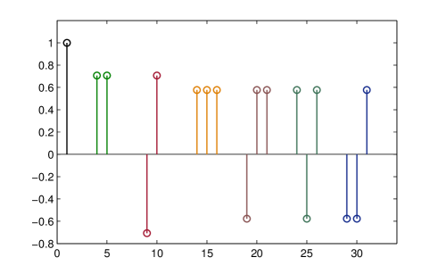
Figure 1: Prototype atoms, which generate the dictionaries $\mathcal{D}_{L}^{x}$ by sequential translations of one point. Each prototype is shown in a different color.

The graphs in Fig.2 depict four different 2D atoms.

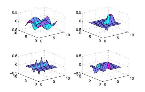
Figure 2: Four different 2D atoms, $\mathbf{d}^{x}_{\ell_{i}}(\mathbf{d}^{y}_{\ell_{j}})^{T}$, with $\mathbf{d}^{x}_{\ell_{i}}$ a member of $\mathcal{D}_{C}^{x}$ and $\mathbf{d}^{y}_{\ell_{j}}$ a member of $\mathcal{D}_{C}^{y}$ (top left graph), $\mathbf{d}^{x}_{\ell_{i}}$ a member of $\mathcal{D}_{L}^{x}$ and $\mathbf{d}^{y}_{\ell_{j}}$ a member of $\mathcal{D}_{L}^{y}$ (top right graph), $\mathbf{d}^{x}_{\ell_{i}}$ a member of $\mathcal{D}_{L}^{x}$ and $\mathbf{d}^{y}_{\ell_{j}}$ a member of $\mathcal{D}_{S}^{y}$ (bottom left graph), $\mathbf{d}^{x}_{\ell_{i}}$ a member of $\mathcal{D}_{C}^{x}$ and $\mathbf{d}^{y}_{\ell_{j}}$ a member of $\mathcal{D}_{L}^{y}$ (bottom right graph)

Remark 1: The mixed dictionary given above is specially suited for approximations in the wavelet domain. Once the approximation of the blocks is concluded, these are assembled to produce the approximated array $\mathbf{U}^{K}=\hat{\operatorname{J}}_{q=1}^{Q}\mathbf{U}_{q}^{k_{q}}$. Finally, the inverse wavelet transform is applied to convert the array $\mathbf{U}^{K}$ into the approximation of the intensity image $\mathbf{I}^{K}$.

Numerical Examples

We illustrate now the suitability of the proposed mixed dictionary to produce high quality approximations of the set of X-ray medical images shown in Fig. 3. This set of twenty images is the Lukas 2D 8 bit medical image corpus, available on [33].

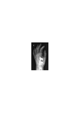
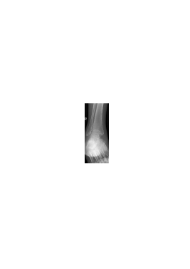
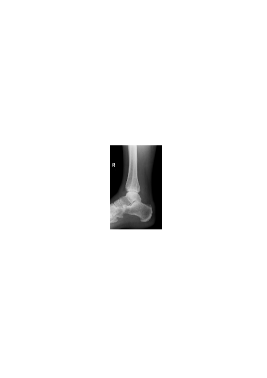
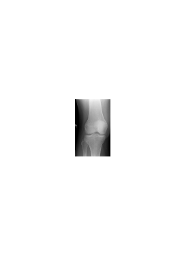
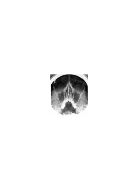
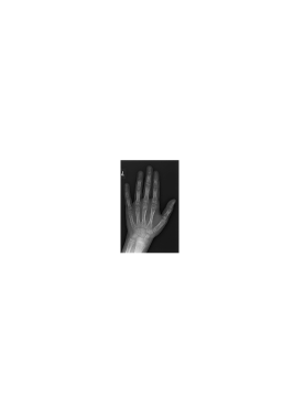
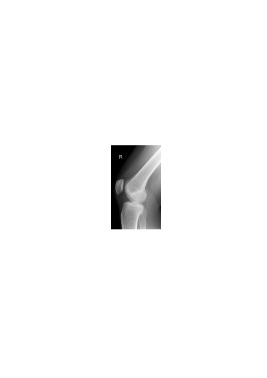
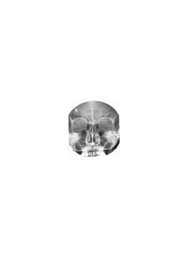
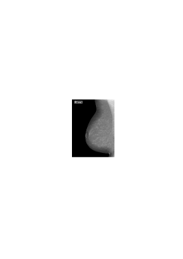
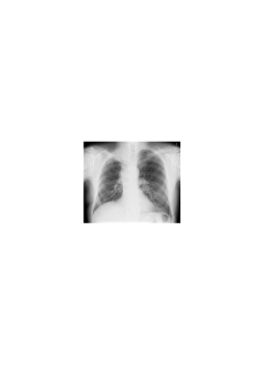
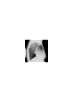
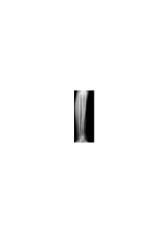
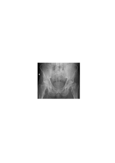
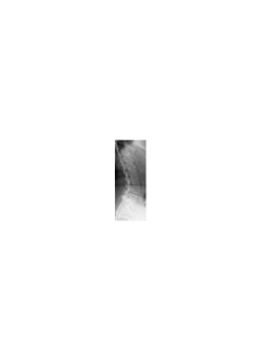
Figure 3: Lukas Corpus [33] listed in Table I. From top to bottom and left to right: Hand₀, Foot₁, Foot₀, Head₀, Knee₁, Sinus₀, Hand₀, Head₁, Knee₀, Sinus₁, Breast₀, Breast₁, Thorax₀, Thorax₁, Leg₀. Leg₁, Pelvis₁, Pelvis₀, Spine₁, Spine₀.

The comparison is performed with respect to the SR achieved by nonlinear thresholding of the DCT and DWT coefficients, respectively, to produce an approximation of the same quality. The quality is set by requiring a value of MSSIM greater than 0.998, and fixing the PSNR as a value for which the DWT approach produces the required MSSIM. The PSNR is more sensitive to small variations in the approximation than the MSSIM. By fixing the PSNR, at the values given in Table I, the equivalence of quality is ensured with respect to both measures. Certainly, in its original size is not possible to distinguish the actual images from their approximations with any of the approaches.

The first column of Table I lists the images in Fig. 3. The second column displays the value of PSNR. The third and forth columns correspond to the SR obtained through the DWT and DCT, respectively. The DWT approximation is calculated by applying the Cohen-Daubechies-Feauveau 9$/$7 (CDF97) wavelet transform on the whole image (using the waveletcdf97 MATLAB routine available on [34]) and reducing coefficients, by iteratively thresholding, to produced the required quality in the pixel-intensity domain. The DCT approximation is calculated by applying the DCT to the intensity image on a partition of block size $8\times 8$ and reducing coefficients in a HBW manner. This procedure and block size yield the best sparsity results using DCT. The images are ordered according to the SR achieved with the DWT approximation. The sparsest is the first image and the least sparse the last one.

The first step in the implementation of the dictionary approximation is to transform the image, for which we use the waveletcdf97 function. For the images in the upper part of the table (from Head₁ to Breast₀) the SR results rendered by this approach, for a partition of block size $8\times 8$, strongly depend on the method used for the selection process. Because those images are sparse in the wavelet domain, the ranking of the blocks for their approximation through the HBW-OMP2D method yields significantly higher SR (sixth column) than the standard application of OMP2D (fifth column).

Image PSNR DWT DCT OMP2D HBW Hand₁ 48.1 30.0 26.4 39.0 72.6 Foot₁ 48.6 26.6 26.1 30.4 44.9 Foot₀ 48.6 25.5 26.1 42.7 65.2 Head₀ 47.4 25.3 24.3 51.9 63.2 Knee₁ 48.0 22.7 23.0 34.5 59.8 Sinus₀ 47.1 18.9 18.7 31.3 46.7 Hand₀ 48.8 18.6 18.7 32.2 47.9 Head₁ 46.4 17.5 15.1 38.3 44.4 Knee₀ 49.1 17.4 17.5 33.2 45.9 Sinus₁ 45.8 17.2 17.1 29.5 43.0 Breast₀ 44.3 15.7 15.3 36.7 41.0 Breast₁ 44.3 11.5 11.2 27.7 29.7 Thorax₀ 44.1 10.6 10.9 25.1 27.4 Thorax₁ 43.4 10.3 9.6 25.4 26.3 Leg₀ 48.9 8.2 8.4 21.2 22.3 Leg₁ 49.2 5.8 5.9 15.1 15.4 Pelvis₁ 44.3 4.8 4.7 12.3 12.6 Pelvis₀ 44.4 4.6 4.7 12.4 12.6 Spine₁ 47.0 3.5 3.6 9.3 9.4 Spine₀ 47.4 2.9 2.8 7.1 7.7

TABLE I: Comparison of the SR calculated by the DWT, DCT, and dictionary approaches. The approximation with DCT and dictionary are carried out on a partition of $8\times 8$ blocks. The values corresponding to the dictionary are those obtained with the OMP2D method and its corresponding HBW version. All the approximations produce a MSSIM greater than 0.998.

The images in the lower part of Table I (from Breast₁ to Spine₀) are less sparse in the wavelet domain, as indicated by the SR produced by the DWT approximation. Thus, even if the dictionary method achieves, for all the images, a very significant gain in SR with respect to the DWT and DCT approaches, the results corresponding to the OMP2D and HBW-OMP2D methods are much closer than they are for the images in the upper part of the table. As can be seen in Table II, the processing time with both methods is very competitive, considering that the results have been produced in a MATLAB environment using C++ MEX files for the OMP2D and HBW-OMP2D routines.

Corpus Mean value size OMP2D HBW X-Ray Lukas $1943\times 1364$ pixels 5.1 secs 10.3 secs

TABLE II: Mean value processing time (per image) to obtain the results of Table I. The second column shows the mean value size of the images in the set. The third column corresponds to the OMP2D method and the forth column to the HWB-OMP2D one. The given times are the average of five independent runs with a single processor in a notebook Core i7 3520M, 4GB RAM.

While for the images in the upper part of the table is worth applying the HBW-OMP2D method, for most of the images in the lower part of the table the difference is not significant. All further results of SR will be presented by grouping the first eleven images (from Hand₁ to Breast₀) in a set, say $\cal{U}$, and the remaining images (from Breast₁ to Spine₀) in a set $\cal{L}$.

For the same quality as in Table I , with the dictionary approach we also consider partitions of block size $16\times 16$ and $24\times 24$. The points in the top graph of Fig. 3 represent the mean vale of the SR with respect to the images in the set $\cal{U}$, vs block size $8\times 8,16\times 16$, and $24\times 24$. In order to facilitate a visual comparison, the DCT and DWT results are simply repeated. They correspond to the best result for the DWT, which occurs when each image is processed as a whole, and the best result for DCT, which occurs for a partition of block size $8\times 8$.

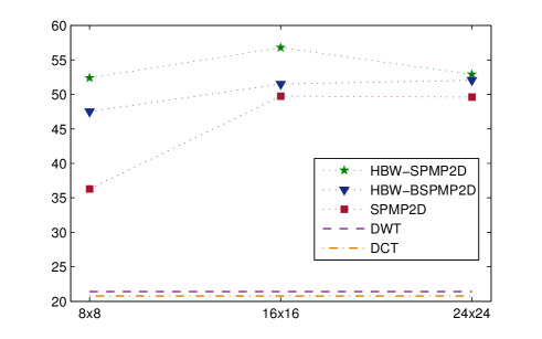
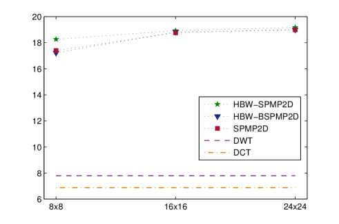
Figure 4: Mean SR vs block size $N_{b}\times N_{b}$ for the X-Ray images in Fig. 3. The green stars are the values obtained with HBW-SPMP2D, the red squares with SPMP2D, and the blue triangles with HBW-BSPMP2D. The dashed line and the dash-dot line represent the DWT and DCT results, respectively. The top graph corresponds to the images in the upper part of Table I (set ${\cal{U}}$) and the bottom one corresponds to the images in the lower part of that table (set ${\cal{L}.}$)

Due to memory requirements, for the images in the set ${\cal{L}}$ and for the partition of block of size $24\times 24$ we can only implement HBW-SPMP2D. Hence, for consistency, the graphs in Fig. 4 have been produced with the SPMP2D and HBW-SPMP2D methods. The red squares correspond to the mean SR value obtained by SPMP2D and the green stars are those obtained by HBW-SPMP2D. The blue triangles in the same graphs are the result of applying a combination of approaches. Firstly, each image is approximated block by block with SPMP2D up to a PSNR $2\%$ higher than the required PSNR. Subsequently, the approximation is downgraded in a HBW fashion to produce the required global PSNR by means of the HBW-BSPMP2D approach, as described in Sec. II-D. The top graph in Fig. 4 corresponds to the images in the set ${\cal{U}}$, and the difference between approaches is noticeable. On the contrary, as seen in the bottom graph corresponding to the images in the set ${\cal{L}}$, except for block size $8\times 8$ all the three methods yield equivalent results.

Remark 2: The numerical tests presented in this section lead to the following conclusions:

• Approximating the set of medical images in Fig. 3 using the proposed mixed dictionary produces a very significant gain in the mean $\mathrm{SR}$ value, in relation to the one yielded by traditional DCT and DWT approximations.

• The best compromise between sparsity and computational time is attained for a partition of block size $16\times 16$. The quantification of the relative gain in SR of one particular approach, in relation to other, is given by the quantity:

  $$\mathrm{G}=\frac{\mathrm{SR}_{A}-\mathrm{SR}_{B}}{\mathrm{SR}_{B}}100\%,$$

  where $\mathrm{SR}_{B}$ is the SR produced by the approach for which the gain is referred to. Accordingly, the mean value sparsity gain in relation to DWT results, including all the twenty images in the set, is $142\%$ with standard deviation of $18\%$. These results can be obtained very effectively through the HBW-OMP2D method, if the images are sparse in the wavelet domain. Otherwise, the OMP2D method is more effective because it produces faster equivalent results. Moreover, parallelization of block approximation with multi-processors is straightforward.

• For blocks larger than $16\times 16$ the methods SPMP2D and HBW-SPMP2D (low memory implementations of OMP2D and HBW-OMP2D respectively) may be required. However, when the approximation is carried out in the wavelet domain blocks of size larger than $16\times 16$ do not improve sparsity in a significant way.

• For partitions of block size $8\times 8$, refining a OMP2D approximation by HBW-BSPMP2D pruning is an option worth consideration, if the image is sparse in the wavelet domain. The actual results vary according to how far the forward selection goes. The results presented here correspond to a slight pruning which degrades the quality of the forward approximation only $2\%$.

• Since the DWT is a fast approximation, it can be used as a tool to help decide the strategy for approximating with dictionaries. If the fast DWT approximation gives a high $\mathrm{SR}$ (say $\mathrm{SR}>10$ for the high quality reconstruction required in this context) then using the HBW version of a pursuit strategy is strongly advised.

Note: All the routines for implementation of the approximation methods and the script for reproducing results have been made available on the website [35].

III Conclusions

Sparse representation of X-Ray medical images in the context of data reduction has been considered. The success of the framework is based on (a) the suitability of the proposed dictionary and (b) the effectiveness of the algorithms for realizing the approximation. The comparison with traditional approaches such as non linear approximations through DWT and DCT redounds in a mean value gain of sparsity of up to $148\%$ (for block size $16\times 16$) which is achieved at a very competitive time (11.4 secs per image) even when the implementation is carried out in a small notebook within a MATLAB environment. The results are really encouraging. We feel confident that the proposed framework will be of assistance to X-ray image processing applications relying on data reduction. In order to facilitate further developments, as well as the reproduction of the results in this paper, the implementation of all the algorithms has been made available on a dedicated website [35].

References

- [1] European Society of Radiology, “Usability of irreversible image compression in radiological imaging”, Insights Imaging 2, 103–115 (2011).
- [2] J. Andreu-Perez, C C. Y. Poon, R. D Merrifield, S. T. C. Wong, G-Z Yang, “Big Data for Health”, IEEE Journal of Biomedical and Health Informatics, 19, 1193–1208, (2015)
- [3] D. L. Donoho, “Compressed sensing”, IEEE Trans. Inf. Theory,52, 1289–1306 (2006).
- [4] E. Candès and M. Wakin, “An introduction to compressive sampling”, IEEE Signal Processing Magazine, 25, 21 – 30 (2008).
- [5] R. Baraniuk, “More Is less: Signal processing and the data deluge”, Science, 331, 717 – 719 (2011).
- [6] B. K. Natarajan, “Sparse Approximate Solutions to Linear Systems”, SIAM Journal on Computing, 24, 227–234 (1995).
- [7] S. S. Chen, D. L. Donoho, and M. A Saunders, “Atomic Decomposition by Basis Pursuit”, SIAM Journal on Scientific Computing, 20, 33–61 (1998).
- [8] M. Elad, Sparse and Redundant Representations: From Theory to Applications in Signal and Image Processing, Springer (2010).
- [9] S. Mallat and Z. Zhang, “Matching pursuit with time-frequency dictionaries,” IEEE Transactions on Signal Processing, Vol (41,12) 3397–3415 (1993).
- [10] Y.C. Pati, R. Rezaiifar, and P.S. Krishnaprasad, “Orthogonal matching pursuit: recursive function approximation with applications to wavelet decomposition,” Proc. of the 27th ACSSC,1,40–44 (1993).
- [11] L. Rebollo-Neira and D. Lowe, “Optimized orthogonal matching pursuit approach”, IEEE Signal Process. Letters, 9, 137–140 (2002).
- [12] M. Andrle, L. Rebollo-Neira, and E. Sagianos, “Backward-optimized orthogonal matching pursuit approach”, IEEE Signal Process. Let.,11,705–708 (2004).
- [13] J. A. Tropp, “Greed is good: algorithmic results for sparse approximation”, IEEE Transactions on Information Theory, 50, 2231–2242 (2004).
- [14] M. Andrle and L. Rebollo-Neira, “A swapping-based refinement of orthogonal matching pursuit strategies”, Signal Processing, 86, 480–495 (2006).
- [15] D. L. Donoho , Y. Tsaig , I. Drori , and J. Starck, “Stagewise Orthogonal Matching Pursuit”, IEEE Transactions on Information Theory, 58, 1094–1121 (2006).
- [16] T. Blumensath, M. E. Davies, “Gradient Pursuits”, IEEE Transactions on Signal Processing, 56, 2370 – 2382 (2008).
- [17] D. Needell and J.A. Tropp, “CoSaMP: Iterative signal recovery from incomplete and inaccurate samples”, Applied and Computational Harmonic Analysis, 26, 301–321 (2009).
- [18] D. Needell and R. Vershynin, “Signal Recovery From Incomplete and Inaccurate Measurements via Regularized Orthogonal Matching Pursuit”, IEEE Journal of Selected Topics in Signal Processing, 4, 310–316 (2010).
- [19] Y. Eldar, P. Kuppinger, and H. Biölcskei, “Block-Sparse Signals: Uncertainty Relations and Efficient Recovery”, IEEE Trans. Signal Process., 58, 3042–3054 (2010).
- [20] L. Rebollo-Neira, R. Matiol, and S. Bibi, “Hierarchized block wise image approximation by greedy pursuit strategies,” IEEE Signal Process. Letters, 20, 1175–1178 (2013).
- [21] L. Rebollo-Neira, “Cooperative greedy pursuit strategies for sparse signal representation by partitioning”, Signal Processing, 125, 365–375 (2016).
- [22] Z. Wang, A. C. Bovik, H. R. Sheikh, E. P. Simoncelli, “Image quality assessment: From error visibility to structural similarity,” IEEE Transactions on Image Processing, 13, 600–612 (2004).
- [23] I. Kowalik-Urbaniak, D. Brunet, J. Wang, D. Koff, N. Smolarski-Koff, E. Vrscay, B. Wallace, and Z. Wang, “The quest for ‘diagnostically lossless’ medical image compression: a comparative study of objective quality metrics for compressed medical images”, Proc. SPIE 9037, Medical Imaging 2014: Image Perception, Observer Performance, and Technology Assessment, 903717 (March 11, 2014); doi:10.1117/12.2043196.
- [24] L. Rebollo-Neira, J. Bowley, A. Constantinides and A. Plastino, “Self contained encrypted image folding”, Physica A, 391, 5858–5870 (2012).
- [25] L. Rebollo-Neira, J.Bowley Sparse representation of astronomical images, Journal of The Optical Society of America A, 30, 758–768 (2013).
- [26] L. Rebollo-Neira, P. Sasmal, “Low memory implementation of Orthogonal Matching Pursuit like greedy algorithms: Analysis and Applications”, http://arxiv.org/abs/1609.00053 (2016)
- [27] K. Kreutz-Delgado, J. F. Murray, B. D. Rao, K. Engan, Te-Won Lee, and T. J. Sejnowski, “Dictionary Learning Algorithms for Sparse Representation”, Neurocomputing, 15, 349–396 (2003).
- [28] M. Aharon, M. Elad, and A. Bruckstein, “K-SVD: An Algorithm for Designing Overcomplete Dictionaries for Sparse Representation”, IEEE Trans. Signal Process. 54, 4311–4322 (2006).
- [29] R. Rubinstein, M. Zibulevsky, and M. Elad, “Double Sparsity: Learning Sparse Dictionaries for Sparse Signal Approximation”, IEEE Trans. Signal Process. 58, 1553–1564 (2010).
- [30] I. Tos̆ić and P. Frossard, “Dictionary Learning: What is the right representation for my signal?”, IEEE Signal Processing Magazine, 28, 27–38 (2011).
- [31] J. Zepeda, C. Guillemot, E. Kijak, “Image Compression Using Sparse Representations and the Iteration-Tuned and Aligned Dictionary”, IEEE Journal of Selected Topics in Signal Processing, 5,1061–1073 (2011).
- [32] M. Srinivas, R. R. Naidu, C.S. Sastry, C. Krishna Mohana, “Content based medical image retrieval using dictionary learning”, Neurocomputing, 168, 880–895 (2015).
-
[33]
http://www.data-compression.info/Corpora/
LukasCorpus/ - [34] http://www.getreuer.info/home/waveletcdf97
-
[35]
http://www.nonlinear-approx.info/examples/
node06.htm