Cluster Mass Calibration at High Redshift: HST Weak Lensing Analysis of 13 Distant Galaxy Clusters from the South Pole Telescope Sunyaev-Zel’dovich Survey
Abstract
We present an HST/ACS weak gravitational lensing analysis of 13 massive high-redshift () galaxy clusters discovered in the South Pole Telescope (SPT) Sunyaev-Zel’dovich Survey. This study is part of a larger campaign that aims to robustly calibrate mass-observable scaling relations over a wide range in redshift to enable improved cosmological constraints from the SPT cluster sample. We introduce new strategies to ensure that systematics in the lensing analysis do not degrade constraints on cluster scaling relations significantly. First, we efficiently remove cluster members from the source sample by selecting very blue galaxies in colour. Our estimate of the source redshift distribution is based on CANDELS data, where we carefully mimic the source selection criteria of the cluster fields. We apply a statistical correction for systematic photometric redshift errors as derived from Hubble Ultra Deep Field data and verified through spatial cross-correlations. We account for the impact of lensing magnification on the source redshift distribution, finding that this is particularly relevant for shallower surveys. Finally, we account for biases in the mass modelling caused by miscentring and uncertainties in the concentration–mass relation using simulations. In combination with temperature estimates from Chandra we constrain the normalisation of the mass–temperature scaling relation to , consistent with self-similar redshift evolution when compared to lower redshift samples. Additionally, the lensing data constrain the average concentration of the clusters to .
keywords:
gravitational lensing: weak – cosmology: observations – galaxies: clusters: general1 Introduction
Constraints on the number density of clusters as a function of their mass and redshift probe the growth of structure in the Universe, therefore holding great promise to constrain cosmological models (e.g. Haiman, Mohr & Holder, 2001; Allen, Evrard & Mantz, 2011; Weinberg et al., 2013). Previous studies using samples of at most a few hundred clusters have delivered some of the tightest cosmological constraints currently available on dark energy properties, theories of modified gravity, and the species-summed neutrino mass (e.g. Vikhlinin et al. 2009b; Rapetti et al. 2009, 2013; Schmidt, Vikhlinin & Hu 2009; Mantz et al. 2010, 2015; Bocquet et al. 2015; de Haan et al. 2016). Recently, CMB experiments have begun to substantially increase the number of massive, high-redshift clusters found with well-characterised selection functions, detected via their Sunyaev-Zel’dovich (SZ, Sunyaev & Zel’dovich, 1970, 1972) signature from inverse Compton scattering off the electrons in the hot cluster plasma (Hasselfield et al., 2013; Bleem et al., 2015; Planck Collaboration et al., 2016a). Upcoming experiments such as SPT-3G (Benson et al., 2014) and eROSITA (Merloni et al., 2012) are expected to soon provide samples of – massive clusters with well-characterised selection functions, yielding a statistical constraining power that may mark the transition between “Stage III” and “Stage IV” dark energy constraints (see Albrecht et al., 2006) from clusters if systematic uncertainties are well controlled.
Cluster observables such as X-ray luminosity, SZ signal, or optical/NIR richness and luminosity have been shown to scale with mass (e.g. Reiprich & Böhringer, 2002; Lin, Mohr & Stanford, 2004; Andersson et al., 2011). In order to adequately exploit the statistical constraining power of large cluster surveys, an accurate and precise calibration of the scaling relations between such mass proxies and mass is needed. Already for current surveys cosmological constraints are primarily limited by uncertainties in the calibration of mass–observable scaling relations (e.g. Rozo et al., 2010; Sehgal et al., 2011; Benson et al., 2013; von der Linden et al., 2014b; Mantz et al., 2015; Planck Collaboration et al., 2016c). It is therefore imperative to improve this calibration empirically. In this context our work focuses especially on calibrating mass–observable relations at high redshifts, which together with low-redshift measurements, provides constraints on their redshift evolution. Particularly for constraints on dark energy properties, which are primarily derived from the redshift evolution of the cluster mass function, it is critical to ensure that systematic errors in the evolution of mass–observable scaling relations do not mimic the signature of dark energy. Most previous cosmological cluster studies had to rely on priors for the redshift evolution derived from numerical cluster simulations (e.g. Vikhlinin et al., 2009b; Benson et al., 2013; de Haan et al., 2016). It is crucial to test the assumed models of cluster astrophysics in these simulations by comparing their predictions to observational constraints on the scaling relations (e.g. Le Brun et al., 2014), and to shrink the uncertainties on the scaling relation parameters.
Progress in the field critically requires improvements in the cluster mass calibration through large multi-wavelength follow-up campaigns. For example, high-resolution X-ray observations provide mass proxies with low intrinsic scatter, which can be used to constrain the relative masses of clusters (e.g. Vikhlinin et al., 2009a; Reichert et al., 2011; Andersson et al., 2011). On the other hand, weak gravitational lensing has been recognised as the most direct technique for the absolute calibration of the normalisation of cluster mass observable relations (Allen, Evrard & Mantz, 2011; Hoekstra et al., 2013; Applegate et al., 2014; Mantz et al., 2015). The main observable is the weak lensing reduced shear, a tangential distortion caused by the projected tidal gravitational field of the foreground mass distribution. It is directly related to the differential projected cluster mass distribution, and can be estimated from the observed shapes of background galaxies (e.g. Bartelmann & Schneider, 2001; Schneider, 2006).
To date, the majority of cluster weak lensing mass estimates have been obtained for lower redshift clusters (–) using ground-based observations (e.g. High et al., 2012; Israel et al., 2012; Oguri et al., 2012; Applegate et al., 2014; Gruen et al., 2014; Umetsu et al., 2014; Hoekstra et al., 2015; Ford et al., 2015; Kettula et al., 2015; Battaglia et al., 2016; Lieu et al., 2016; van Uitert et al., 2016; Okabe & Smith, 2016; Simet et al., 2017; Melchior et al., 2017). To constrain the evolution of cluster mass-observable scaling relations, these measurements need to be complimented with constraints for higher redshift clusters. Here, ground-based measurements suffer from low densities of sufficiently resolved background galaxies with robust shape measurements. This can be overcome using high-resolution Hubble Space Telescope (HST) images, where so far Jee et al. (2011) present the only weak lensing constraints for the cluster mass calibration of a large sample of massive high-redshift () clusters, which were drawn from optically, NIR, and X-ray-selected samples. Interestingly, their results suggest a possible evolution in the scaling relation in comparison to self-similar extrapolations from low redshifts, with lower masses at the level. HST weak lensing measurements have also been used to constrain mass-observable scaling relations for lower (Leauthaud et al., 2010) and intermediate mass clusters (Hoekstra et al., 2011a).
This paper is part of a larger effort to obtain improved observational constraints on the calibration of cluster masses as function of redshift. Here we analyse new HST observations of 13 massive high- clusters detected by the South Pole Telescope (Carlstrom et al., 2011) via the SZ effect. This constitutes the first high- sample of clusters with HST weak lensing observations which were drawn from a single, well-characterised survey selection function. As a major part of this paper, we carefully investigate and account for the relevant sources of systematic uncertainty in the weak lensing mass analysis, and discuss their relevance for future studies of larger samples.
The primary technical challenges for weak lensing studies are accurate measurements of galaxy shapes from noisy data in the presence of instrumental distortions, and the need for an accurate knowledge of the source redshift distribution which enters through the geometric lensing efficiency. Within the weak lensing community substantial progress has been made on the former issue through the development of improved shape measurement algorithms tested using image simulations (e.g. Miller et al., 2013; Hoekstra et al., 2015; Bernstein et al., 2016; Fenech Conti et al., 2017). For the latter issue, previous studies have typically estimated the redshift distribution from photometric redshifts (photo-s) given the incompleteness of spectroscopic redshift samples (spec-s) at the relevant magnitudes, requiring that the photo--based estimates are sufficiently accurate. If sufficient wavelength coverage is available, photo-s can be estimated directly for the weak lensing survey fields of interest (used in the cluster context e.g. by Leauthaud et al., 2010; Applegate et al., 2014; Ford et al., 2015). Otherwise, photo-s can be used from external reference deep fields, requiring that statistically consistent and sufficiently representative galaxy populations are selected in both the survey and reference fields. For cluster weak lensing studies both approaches are complicated by the fact that the presence of a cluster means that the corresponding line-of-sight is over-dense at the cluster redshift, while both the default priors of photo- codes and the reference deep fields ought to be representative for the cosmic mean distribution. Previous studies employing reference fields have typically dealt with this issue by applying colour selections (“colour cuts”) that remove galaxies at the cluster redshift (e.g. High et al., 2012; Hoekstra et al., 2012; Okabe & Smith, 2016). In case of incomplete removal the approach can be complemented by a statistical correction for the residual cluster member contamination if that can be estimated sufficiently well (e.g. Hoekstra et al., 2015). For cluster weak lensing studies a further complication arises when parametric models are fitted to the measured tangential reduced shear profiles, as issues such as miscentring (e.g. Johnston et al., 2007; George et al., 2012) or uncertainties regarding assumed cluster concentrations can lead to non-negligible biases, introducing the need for calibrations using simulations (e.g. Becker & Kravtsov, 2011).
This paper is organised as follows: Sect. 2 summarises relevant aspects of weak lensing theory. This is followed by a description of our cluster sample in Sect. 3 and a description of the analysed data and image processing in Sect. 4. Sect. 5 details on the weak lensing shape measurements and a new test for signatures of potential residuals of charge-transfer inefficiency in the weak lensing catalogues. In Sect. 6 we describe in detail our approach to remove cluster galaxies via colour cuts and reliably estimate the source redshift distribution using data from the CANDELS fields. In Sect. 7 we present our weak lensing shear profile analysis, mass reconstructions, and mass estimates, which we use in Sect. 8 to constrain the mass–temperature scaling relation. Finally, we discuss our findings in Sect. 9 and conclude in Sect. 10.
Throughout this paper we assume a standard flat CDM cosmology characterised by , , and km/s/Mpc with , as approximately consistent with recent CMB constraints (Hinshaw et al., 2013; Planck Collaboration et al., 2016b). For the computation of large-scale structure noise on the weak lensing estimates and the concentration–mass relation according to Diemer & Kravtsov (2015) we furthermore assume , , and . All magnitudes are in the AB system and are corrected for extinction according to Schlegel, Finkbeiner & Davis (1998).
2 Summary of Relevant Weak Lensing Theory
The images of distant background galaxies are distorted by the tidal gravitational field of a foreground mass concentration, see e.g. the reviews by Bartelmann & Schneider (2001); Schneider (2006), as well as Hoekstra et al. (2013) in the context of galaxy clusters. In the weak lensing regime the size of a source is much smaller than the characteristic scale on which variations in the tidal field occur. In this case the lens mapping as function of observed position can be described using the reduced shear and the convergence , which is the ratio of the surface mass density and the critical surface mass density
| (1) |
with the speed of light , the gravitational constant , and the geometric lensing efficiency
| (2) |
where , , and indicate the angular diameter distances to the source, to the lens, and between lens and source, respectively. The reduced shear
| (3) |
describes the observable anisotropic shape distortion due to weak lensing. It is a two component quantity, conveniently written as a complex number
| (4) |
where constitutes the strength of the distortion and its orientation with respect to the coordinate system. The reduced shear is a rescaled version of the unobservable shear , and can be estimated from the ensemble-averaged PSF-corrected ellipticities of background galaxies (see Sect. 5), with the expectation value
| (5) |
Due to noise from the intrinsic galaxy shape distribution and measurement noise we need to average the ellipticities of a large ensemble of galaxies
| (6) |
to obtain useful constraints, where indicates the two ellipticity components and indicates galaxy . The shape weights are included to improve the measurement signal-to-noise ratio, where contains contributions both from the measurement noise and the intrinsic shape distribution (see Appendix A, where we constrain both contributions empirically using CANDELS data).
It is often useful to decompose the shear, reduced shear, and the ellipticity into their tangential components, e.g. , and cross components, e.g. , with respect to the centre of a mass distribution as
| (7) | |||||
| (8) |
where is the azimuthal angle with respect to the centre. The azimuthal average of the tangential shear at a radius around the centre of the mass distribution is linked to the mean convergence inside and at via
| (9) |
The weak lensing convergence and shear scale for an individual source galaxy at redshift with the geometric lensing efficiency , which is often conveniently written as
| (10) |
where and correspond to the values for a source at infinite redshift, and . In practise, we average the ellipticities of an ensemble of galaxies distributed in redshift, providing an estimate for
| (11) |
While one could in principle compute the exact model prediction for this from the source redshift distribution weighted by the lensing weights, a sufficiently accurate approximation is provided in Hoekstra, Franx & Kuijken (2000):
| (12) |
(see also Seitz & Schneider, 1997; Applegate et al., 2014), where
| (13) |
need to be computed from the estimated source redshift distribution, taking the shape weights into account.
When the signal of lenses at different redshifts is compared or stacked, it can be useful to conduct the analysis in terms of the differential surface mass density
| (14) |
to compensate for the redshift dependence of the signal, where the the summation is conducted over sources in a separation interval around .
Gravitational lensing leaves the surface brightness invariant. Accordingly, a relative change in the observed flux of a source due to lensing is solely given by the relative magnification of the source
| (15) |
Together with the change in solid angle this also changes the observed density of background sources and their redshift distribution, as investigated in Sect. 6.7.
3 The Cluster Sample
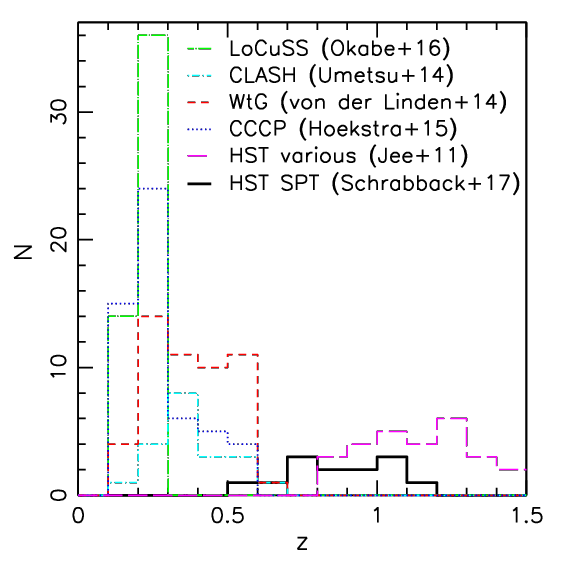
We study a total of 13 distant galaxy clusters detected by the SPT in the redshift range via the SZ effect; see Table 1 for details and Fig. 1 for a comparison of the cluster redshift distribution to recent large weak lensing cluster samples from the Canadian Cluster Comparison Project (CCCP; Hoekstra et al., 2015), Weighing the Giants (WtG; von der Linden et al., 2014a), the Cluster Lensing And Supernova survey with Hubble (CLASH; Umetsu et al., 2014), the Local Cluster Substructure Survey (LoCuSS; Okabe & Smith, 2016), and the analysis of HST observations of X-ray, optically, and NIR selected high-redshift clusters by Jee et al. (2011).
The SPT clusters were observed in HST Cycles 18 and 19. At the time of the target selection, the SPT cluster follow-up campaign was still incomplete. From the clusters with measured spectroscopic redshifts prior to the corresponding cycle, we selected the most massive SPT-SZ clusters at for the Cycles 18 programme, and the most massive clusters at for the Cycle 19 programme. Nine clusters in our overall sample originate from the first 178 deg2 of the sky surveyed by SPT (Vanderlinde et al., 2010, hereafter V10). Using updated estimates of the SZ detection significance from the cluster catalogue for the full 2,500 deg2 SPT-SZ survey (Bleem et al., 2015, hereafter B15), our selection of clusters from the V10 sample includes all clusters from the first 178 deg2 at with plus all clusters at with (see Table 1), except for SPT-CL 05405744 (). Additionally, our sample includes all clusters at from Williamson et al. (2011, henceforth W11), who present a catalogue of the 26 most significant SZ cluster detections in the full 2500 deg2 SPT survey region. This adds three clusters in addition to SPT-CL 23375942, which is part of both samples. Finally, with SPT-CL 20405725 a single further cluster is included from Reichardt et al. (2013, hereafter R13), who present the cluster sample constructed from the first 720 deg2 of the SPT cluster survey. In addition to the aforementioned sample papers, more detailed studies of individual clusters were published for SPT-CL J05465345 (Brodwin et al., 2010) and SPT-CL J21065844 (Foley et al., 2011). Spectroscopic cluster redshift measurements are described in Ruel et al. (2014) and Bayliss et al. (2016). In Table 1 we also list X-ray centroids as estimated from the available Chandra or XMM-Newton data (detailed in Andersson et al., 2011; Benson et al., 2013; McDonald et al., 2013; Chiu et al., 2016b, see also Sect. 8), and BCG positions from Chiu et al. (2016b).
| Cluster name | Coordinates centres [deg J2000] | Sample | ||||||||
|---|---|---|---|---|---|---|---|---|---|---|
| SZ | SZ | X-ray | X-ray | BCG | BCG | [] | ||||
| SPT-CL 00005748 | 0.702 | 8.49 | 0.2499 | 0.2518 | 0.2502 | V10 | ||||
| SPT-CL 01024915 | 0.870 | 39.91 | 15.7294 | 15.7350 | 15.7407 | W11 | ||||
| SPT-CL 05335005 | 0.881 | 7.08 | 83.4009 | 83.4018 | 83.4144 | V10 | ||||
| SPT-CL 05465345 | 1.066 | 10.76 | 86.6525 | 86.6532 | 86.6569 | V10 | ||||
| SPT-CL 05595249 | 0.609 | 10.64 | 89.9251 | 89.9357 | 89.9301 | V10 | ||||
| SPT-CL 06155746 | 0.972 | 26.42 | 93.9650 | 93.9652 | 93.9656 | W11 | ||||
| SPT-CL 20405725 | 0.930 | 6.24 | 310.0573 | 310.0631∗ | 310.0552 | R13 | ||||
| SPT-CL 21065844 | 1.132 | 22.22 | 316.5206 | 316.5174 | 316.5192 | W11 | ||||
| SPT-CL 23315051 | 0.576 | 10.47 | 352.9608 | 352.9610 | 352.9631 | V10 | ||||
| SPT-CL 23375942 | 0.775 | 20.35 | 354.3523 | 354.3516 | 354.3650 | V10, W11 | ||||
| SPT-CL 23415119 | 1.003 | 12.49 | 355.2991 | 355.3009 | 355.3014 | V10 | ||||
| SPT-CL 23425411 | 1.075 | 8.18 | 355.6892 | 355.6904 | 355.6913 | V10 | ||||
| SPT-CL 23595009 | 0.775 | 6.68 | 359.9230 | 359.9321 | 359.9324 | V10 | ||||
Note. — Basic data from Bleem et al. (2015) and Chiu et al. (2016b) for the 13 clusters targeted in this weak lensing analysis. Column 1: Cluster designation. Column 2: Spectroscopic cluster redshift. Column 3: Peak signal-to-noise ratio of the SZ detection. Columns 4–9: Right ascension and declination of the cluster centres used in the weak lensing analysis from the SZ peak, X-ray centroid, and BCG position. ∗: X-ray centroid from XMM-Newton data, otherwise Chandra (see Sect. 8). Column 10: Mass derived from the SZ-Signal. Column 11: SPT parent sample for HST follow-up selection.
4 Data and data reduction
In this section we provide details on the data analysed in this study and their reduction. For the SPT clusters we make use of HST observations (Sect. 4.1.1) for shape and colour measurements, as well as VLT observations (Sect. 4.2) for colour measurements in the outer cluster regions. To optimise our weak lensing pipeline, and to be able to apply consistent selection criteria to photo- catalogues from Skelton et al. (2014), we also process HST observations of the CANDELS fields (Sect. 4.1.3).
4.1 HST/ACS data
4.1.1 SPT cluster observations
We measure weak lensing galaxy shapes from high-resolution Hubble Space Telescope imaging obtained during Cycles 18 and 19 as part of programmes 12246 (PI: C. Stubbs) and 12477111This program also includes observations of SPT-CL J02055829 (). However, we do not include it in the current analysis given its high-redshift, which would require deeper -band observations for the background selection (see Sect. 6) than currently available. (PI: F. W. High), and observed between Sep 29, 2011 and Oct 24, 2012 under low sky background conditions. Each cluster was observed with a ACS/WFC mosaic in the F606W filter, where each tile consists of 4 dithered exposures of 480 s, adding to a total exposure time of 1.92 ks per tile. These mosaic observations allow us to probe the cluster weak lensing signal out to approximately the virial radius. Additionally, a single tile was observed with ACS in the F814W filter on the cluster centre (1.92 ks). These data are included in our photometric analysis (Sect. 6). For the weak lensing shape measurements we chose observations in the F606W filter as it is the most efficient ACS filter in terms of weak lensing galaxy source density (see, e.g. Schrabback et al., 2007). However note that our analysis in Appendix A.4 suggests that future programmes could benefit from mosaic observations in both F606W and F814W to simultaneously obtain robust shape measurements and colour estimates. In fact, a F814W ACS mosaic was obtained for one of the clusters in our sample, SPT-CL 06155746, through the independent HST programme 12757 (PI: Mazzotta), with observations conducted Jan 19–22, 2012. For the current analysis we include these additional data in the colour measurements but not the shape analysis.
We denote magnitudes measured from the ACS F606W and F814W images as and , respectively. By default these correspond to magnitudes measured in circular apertures with a diameter 07 unless explicitly stated differently.
4.1.2 HST data reduction
For basic image reductions we largely employ the standard ACS calibration pipeline CALACS. The main exception is our use of the Massey et al. (2014, M14 henceforth) algorithm for the correction of charge-transfer inefficiency (CTI). CTI constitutes an important systematic effect for HST weak lensing shape analyses if left uncorrected (e.g. Rhodes et al., 2007; Schrabback et al., 2010, S10 henceforth). It is caused by radiation damage in space. The resulting CCD defects act as charge traps during the read-out process, introducing non-linear charge-trails behind objects in the parallel-transfer read-out direction. M14 updated their time-dependent model of the charge trap densities by fitting charge trails behind hot pixels in CANDELS ACS/F606W imaging exposures of the COSMOS field (Grogin et al., 2011), which were obtained at a similar epoch as our cluster data (between Dec 06, 2011 and Apr 15, 2012). Given that we conduct the CTI correction using the M14 code, we also have to CTI-correct the master dark frames using this pipeline. As further differences to standard CALACS processing we compute accurately normalised r.m.s. noise maps as detailed in S10 and optimise the bad pixel mask, where we flag satellite trails and cosmic ray clusters, and unflag the removed CTI trails of hot pixels.
The further data reduction for the individual ACS tiles closely follows S10, to which we refer the reader for details. As the first step, we carefully refine relative shifts and rotations between the exposures by matching the positions of compact objects. We then use MultiDrizzle (Koekemoer et al., 2003) for the cosmic ray removal and stacking, where we employ the lanczos3 kernel at the native pixel scale 005 to minimise noise correlations while only introducing a low level of aliasing for ellipticity measurements (Jee et al., 2007). The pipeline also generates correctly scaled r.m.s. noise maps for stacks that are used for the object detection. We conduct weak lensing shape measurements on these individual stacked ACS tiles (see Sect. 5).
For the joint photometric analysis with available VLT data (Sect. 6.4 with details given in Appendix D) we additionally generate stacks for the ACS mosaics. Here we iteratively align neighbouring tiles by first resampling them separately onto a common pixel grid, only stacking the exposures of the corresponding tile. We then use the differences between the positions of matched objects in the overlapping regions to compute shifts and rotations, in order to update the astrometry.
4.1.3 CANDELS HST data
When estimating the redshift distribution of our source sample (see Sect. 6) we need to apply the same selection function (consisting of photometric, shape, and size cuts) to the galaxies in the CANDELS fields, which act as our reference sample. To be able to employ consistent weak lensing cuts, we reduce and analyse ACS imaging in the CANDELS fields with the same pipeline as the HST observations of the SPT clusters. This includes data from the CANDELS (Grogin et al., 2011, Proposal IDs 12440, 12064), GOODS (Giavalisco et al., 2004, Proposal IDs 9425, 9583), GEMS (Rix et al., 2004, Proposal ID 9500), and AEGIS (Davis et al., 2007, Proposal ID 10134) programmes. Here we perform a tile-wise analysis, always stacking exposures with good spatial overlap which add to approximately 1-orbit depth, roughly matching the depth of our cluster field data (see Appendix A.2 for additional information).
We use these blank field data also as a calibration sample to derive an empirical weak lensing weighting scheme that is based on the measured ellipticity dispersion as function of logarithmic signal-to-noise ratio and employed in our cluster lensing analysis (see Appendix A.5). This analysis also provides updated constraints on the dispersion of the intrinsic galaxy ellipticities and allows us to compare the weak lensing performance of the ACS F606W and F814W filters, aiding the preparation of future weak lensing programmes (see Appendix A.4).
4.2 VLT/FORS2 data
For our analysis we make use of VLT/FORS2 imaging of all of our targets taken as part of programmes 086.A-0741 (PI: Bazin), 088.A-0796 (PI: Bazin), 088.A-0889 (PI: Mohr), and 089.A-0824 (PI: Mohr) in the pass-band, which we call . The FORS2 focal plane is covered with two MIT CCDs. The data were taken with the standard resolution collimator in binning, providing imaging over a field-of-view with a pixel scale of 025, matching the size of our ACS mosaics well.
| Cluster name | IQ | Used range | |||
|---|---|---|---|---|---|
| bright cut | faint cut | ||||
| SPT-CL 00005748 | 2.1 ks | 26.0 | 065 | 24.0–25.5 | 25.5–26.0 |
| SPT-CL 01024915 | 2.1 ks | 25.8 | 075 | 24.0–25.0 | 25.0–25.5 |
| SPT-CL 05335005 | 2.1 ks | 25.8 | 073 | 24.0–25.5 | - |
| SPT-CL 05465345 | 2.1 ks | 25.7 | 075 | 24.0–25.0 | 25.0–25.5 |
| SPT-CL 05595249 | 1.9 ks | 25.6 | 065 | 24.0–25.0 | 25.0–25.5 |
| SPT-CL 06155746 | 2.5 ks | 25.6 | 093 | 24.0–24.5 | 24.5–25.5 |
| SPT-CL 20405725 | 2.9 ks | 25.7 | 070 | 24.0–25.0 | 25.0–25.5 |
| SPT-CL 21065844 | 4.8 ks | 25.8 | 080 | 24.0–25.0 | 25.0–25.5 |
| SPT-CL 23315051 | 2.4 ks | 25.9 | 083 | 24.0–25.5 | 25.5–26.0 |
| SPT-CL 23375942 | 2.1 ks | 25.7 | 080 | 24.0–25.5 | 25.5–26.0 |
| SPT-CL 23415119 | 2.1 ks | 25.8 | 080 | 24.0–25.5 | 25.5–26.0 |
| SPT-CL 23425411 | 2.1 ks | 25.7 | 093 | 24.0–25.0 | 25.0–25.5 |
| SPT-CL 23595009 | 2.1 ks | 25.9 | 068 | 24.0–25.5 | 25.5–26.0 |
Note. — Details of the analysed VLT/FORS2 imaging data. Column 1: Cluster designation. Column 2: Total co-added exposure time. Column 3: -limiting magnitude computed for 15 apertures in the stack from the single pixel noise r.m.s. values of the contributing exposures. Column 4: Image Quality defined as from Source Extractor. Column 5: magnitude range with low photometric colour scatter , for which the “bright” colour cut is applied (see Table 11 in Appendix D). Column 6: magnitude range with increased photometric colour scatter , for which the “faint” colour cut is applied (see Table 11 in Appendix D).
We reduced the data using theli (Erben et al., 2005; Schirmer, 2013), applying bias and flat-field correction, relative photometric calibration, and sky background subtraction using Source Extractor (Bertin & Arnouts, 1996). We use the object positions in the HST F606W image as astrometric reference for the distortion correction. For an initial absolute photometric calibration using the stars located in the central HST tile we employ the relation
| (16) |
which was derived employing the Pickles (1998) stellar library. This relation is valid for and assumes total magnitudes for the computation of . We list total exposure times, limiting magnitudes, and delivered image quality for the co-added images in Table 2. For further details on the data reduction see Chiu et al. (2016b), who also analyse observations obtained with FORS2 in the and pass-bands. In our analysis we do not include these additional bands. Our initial testing indicates that their inclusion would only yield a minor increase in the usable background galaxy source density given the depth of the different observations and typical colours of the dominant background source population.
5 Weak lensing galaxy shapes
5.1 Shape measurements
For the generation of weak lensing shape catalogues we employ the pipeline from S10, which was successfully used for cosmological weak lensing measurements that typically have more stringent requirements on the control of systematics than cluster weak lensing studies. We refer the reader to this publication for a more detailed pipeline description. Here we summarise the main steps and provide details on recent changes to our pipeline only. One of the main changes is the application of the pixel-based CTI correction from M14 (Sect. 4.1.2), which is more accurate than the catalogue-level correction employed in S10. This change has become necessary as we analyse more recent ACS data with stronger CTI degradation.
As the first step in the catalogue generation we use Source Extractor (Bertin & Arnouts, 1996) to detect objects in the F606W stacks and measure basic object properties. For the ellipticity measurement and correction for the point-spread function (PSF) we employ the KSB+ formalism (Kaiser, Squires & Broadhurst, 1995; Luppino & Kaiser, 1997; Hoekstra et al., 1998) as implemented by Erben et al. (2001) with modifications from Schrabback et al. (2007) and S10. We interpolate the spatially and temporally varying ACS PSF using a model derived from a principal component analysis of PSF variations in dense stellar fields. S10 showed that the dominant contribution to ACS PSF ellipticity variations can be described with a single principal component (related to the HST focus position). This one-parameter PSF model is sufficiently well constrained by the high- stars available for PSF measurements in extragalactic ACS pointings. We obtain a PSF model for each contributing exposure based on stellar ellipticity and size measurements in the image prior to resampling (to minimise noise), from which we compute the combined model for the stack. For the current work we recalibrated this algorithm using archival ACS F606W stellar field observations taken after Servicing Mission 4. We processed these data with the same CTI correction method as our cluster field data.
Following S10 we select galaxies in terms of their half-light radius , where is the upper limit of the pixel wide stellar locus, and “pre-seeing” shear polarisability tensor with . Deviating from S10 we exclude very extended galaxies with pixels, as they are poorly covered by the employed postage stamps. As done in S10 we mask galaxies close to the image boundaries, large galaxies, or bright stars.
S10 introduced an empirical correction for noise bias in the ellipticity measurement as a function of the KSB signal-to-noise ratio from Erben et al. (2001). S10 calibrated this correction using simulated images of ground-based weak lensing observations from STEP2 (Massey et al., 2007), and verified that the same correction robustly corrects simulated high-resolution ACS-like weak lensing data with less than 2% residual multiplicative ellipticity bias ( on average). However, as recently shown by Hoekstra et al. (2015), the STEP2 image simulations lack sources at the faint end, affecting the derived bias calibration (see also Hoekstra, Viola & Herbonnet, 2017). Also, deviations in the assumed intrinsic galaxy shape distribution influence the noise-bias correction (e.g. Viola, Kitching & Joachimi, 2014). To minimise the impact of such uncertainties we apply a more conservative galaxy selection requiring from Source Extractor222This cut is more conservative than the cut from S10, which is based on the Erben et al. (2001) signal-to-noise ratio definition that includes a radial weak lensing weight function. approximately corresponds to for our typical source galaxies, but note that there is a significant scatter between both estimates due to the different radial weighting.. To be conservative, we additionally double the systematic uncertainty for the shear calibration in the error-budget of our current cluster study (4%), which is comparable to the mean shear calibration correction of the galaxies passing our cuts (average factor 1.05). In the context of cluster weak lensing studies a relevant question is also if the image simulations probe the relevant range of shears sufficiently well. We expect that this is not a major concern for our study given that for all of our clusters within the radial range used for the mass constraints (see Sect. 7). For comparison, the basic KSB+ implementation used in our analysis was tested in Heymans et al. (2006) using shears up to , where no indications were found for significant quadratic shear bias terms that would result in an inaccurate correction using our linear correction scheme.
We apply the same shape measurement pipeline to the CANDELS data discussed in Sect. 4.1.3. When mimicking our cluster field selection in these catalogues and assigning weights, we rescale the values prior to the cut to account for slight differences in depth. Hence, if a CANDELS tile is slightly shallower (deeper) compared to the cluster tile considered, we will apply a correspondingly slightly lower (higher) cut in the CANDELS tile to select consistent galaxy samples. On average the depth of our CANDELS stacks agrees well with the depth of the cluster field stacks (to 0.065 mag). Together with the fact that depends only weakly on for our colour-selected sample at the faint end (see Sect. 6.5), we therefore ignore second-order effects such as incompleteness differences between the CANDELS and cluster field catalogues.
5.2 Test for residual CTI signatures in the ACS cluster data
CTI generates charge-trails behind objects dominantly in the parallel-transfer readout direction. For raw ACS images this corresponds to the -direction, and this is approximately also the case for distortion-corrected images if MultiDrizzle is run using the native detector orientation. M14 test the performance of their pixel-based CTI correction by averaging the PSF-corrected ellipticity estimates of galaxies in blank field CANDELS data. Images without CTI correction show a prominent alignment with the -axis (), where the magnitude of the effect increases with the -separation relative to the readout amplifiers. In contrast, this alignment is undetected if the correction is applied.
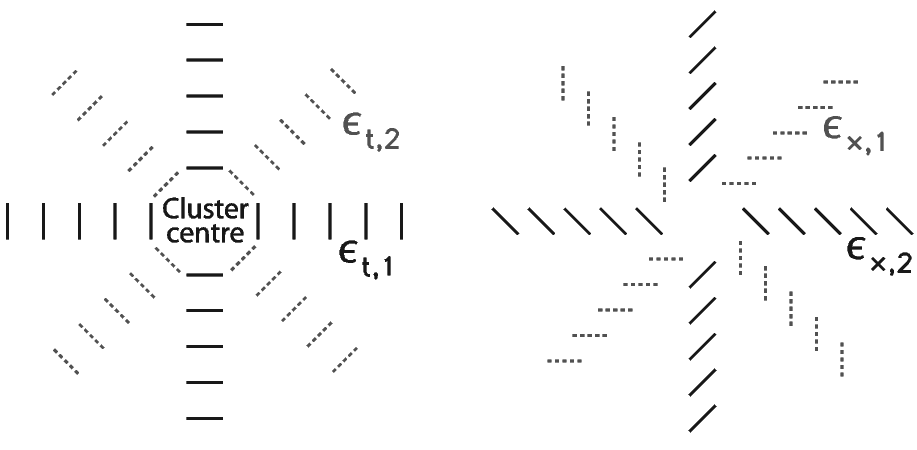
We cannot apply the same test to our ACS data of the cluster fields given the presence of massive clusters, which are always located at the same position within the mosaics, and whose weak gravitational lensing shear would add to the saw-tooth CTI signature. However, we can make use of the fact that CTI primarily affects the ellipticity component (measured along the image axes) but not the ellipticity component (measured along the field diagonals). The tangential and cross components of the ellipticity with respect to the cluster centre
| (17) | |||||
| (18) |
(compare Equations 7 and 8) receive contributions from both ellipticity components with
| (19) | |||||
| (20) | |||||
| (21) | |||||
| (22) |
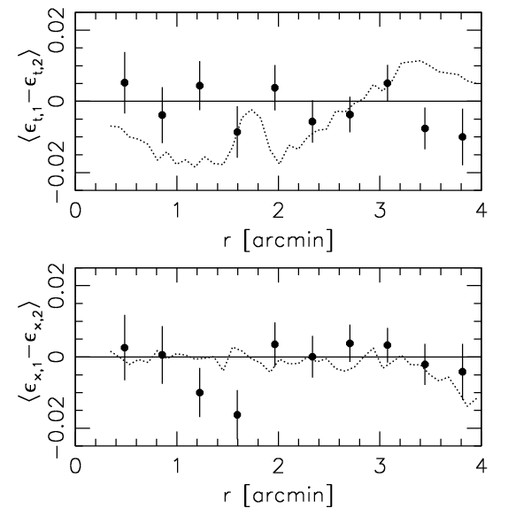
see the sketch in the top panel of Fig. 2 for an illustration of these components. In our test we stack the signal from all clusters. Here we expect that any anisotropy in the reduced shear pattern due to cluster halo ellipticity will average out leading to an approximately circularly symmetric shear field. Accordingly, in the absence of residual systematics we expect that and are consistent with zero when averaged azimuthally. Fig. 2 shows that this is indeed the case for our data (), confirming the success of the CTI correction within the statistical precision of the data. For comparison, the dotted line in Fig. 2 shows the signal that would be caused by a typical uncorrected CTI ellipticity saw-tooth pattern with 333M14 measure an average uncorrected CTI-induced galaxy ellipticity at of from CANDELS/COSMOS F606W images, which were observed at a similar epoch but have higher background levels than our data, and thus weaker CTI signals..
6 Cluster member removal and estimation of the source redshift distribution
Robust weak lensing mass measurements require accurate knowledge of the mean geometric lensing efficiency of the source sample and its variance (see Sect. 2). For a given cosmological model these depend only on the source redshift distribution and cluster redshift. Surveys with sufficiently deep imaging in sufficiently many bands can attempt to estimate the probability distribution of source redshifts directly via photo-s (e.g. Applegate et al., 2014). However, such data are not available for our cluster fields. Hence, we have to rely on an estimate of the redshift distribution from external reference fields. Here we use photometric redshift estimates for the CANDELS fields from the 3D-HST team (Skelton et al., 2014) as primary data set (see Sect. 6.1). Additionally, we use spectroscopic and grism redshift estimates for galaxies in the CANDELS fields, as well as much deeper data from the Hubble Ultra Deep field (HUDF) to investigate and statistically correct for systematic features in the CANDELS photo-s (Sect. 6.3).
Given that our cluster fields are over-dense at the cluster redshift we have to apply a colour selection that robustly removes galaxies at the cluster redshift both in the reference catalogue and our actual cluster field catalogues. Here we use colour estimates from the HST/ACS F606W and F814W images in the inner regions (“ACS-only” selection, Sect. 6.2), and we use VLT/FORS2 -band imaging for the cluster outskirts (“ACS+FORS2” selection, Sect. 6.4 with details given in Appendix D). As discussed in Appendix E we also explored a different analysis scheme which substitutes the colour selection with a statistical correction for cluster member contamination, but we found that we could not control the systematics of the correction to the needed level due to the limited radial range probed by the F606W images. We optimise the analysis by splitting the colour-selected sources into magnitude bins (Sect. 6.5), investigate the influence of line-of-sight variations (Sect. 6.6), and account for weak lensing magnification (Sect. 6.7). Sect. 6.8 presents consistency checks for our analysis based on the source number density measured as function of magnitude and cluster-centric distance.
6.1 CANDELS photometric redshift reference catalogues from 3D-HST
We make use of photometric redshift catalogues computed by the 3D-HST team (Brammer et al., 2012; Skelton et al., 2014, hereafter S14) for the CANDELS fields (Grogin et al., 2011), which consist of five independent lines-of-sight (AEGIS, COSMOS, GOODS-North, GOODS-South, UDS). Hence, their combination efficiently suppresses the impact of sampling variance. All CANDELS field were observed by HST with ACS and WFC3, including ACS F606W and F814W444For the GOODS-North field we estimate the magnitudes from the S14 flux measurements in the F775W and F850LP filters. When conducting selections or binning in based on the S14 photometry we undo their correction for total magnitudes in order to employ aperture magnitudes that are consistent with our cluster field measurements. imaging mosaics that have at least the depth of our cluster field observations (see Koekemoer et al., 2011). This includes observations from the CANDELS program (Grogin et al., 2011) and earlier projects (Giavalisco et al., 2004; Rix et al., 2004; Davis et al., 2007; Scoville et al., 2007). The S14 catalogues are based on detections from combined HST/WFC3 NIR F125W+F140W+F160W images, and include photometric measurements from a total of 147 distinct imaging data sets from HST, Spitzer, and ground-based facilities with a broad wavelength coverage from ( data sets per field). S14 compute photometric redshifts using EAZY (Brammer, van Dokkum & Coppi, 2008), which fits the observed SED constraints of each object with a linear combination of galaxy templates.
We have matched the S14 catalogues with our F606W-detected shape catalogues of the CANDELS fields (see Sect. 5). After applying weak lensing cuts, accounting for masks, and restricting the analysis to the overlap region of the ACS and WFC3 mosaics, we find that of the galaxies in the shape catalogues with have a direct match within 05 in the S14 catalogues, showing that they are nearly complete within our employed magnitude range (see Appendix B for an investigation of the of non-matching galaxies which shows that they have a negligible impact).
6.2 Source selection using ACS-only colours
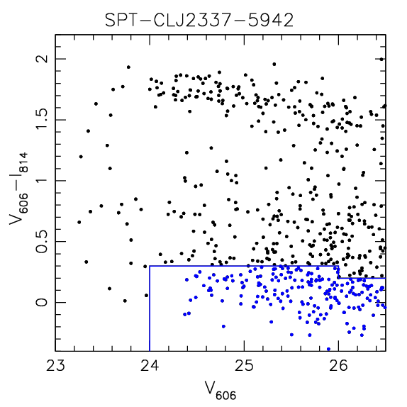
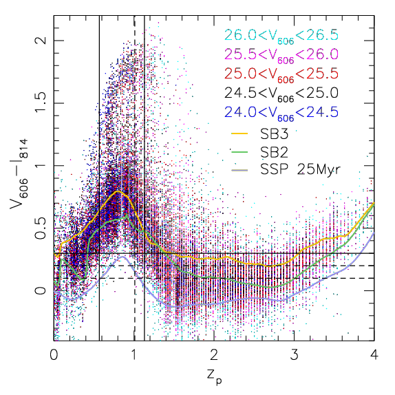
In the inner cluster regions we apply a colour selection (indicated in Fig. 3) using our ACS F606W and F814W images, selecting only galaxies that are bluer than nearly all galaxies at the cluster redshift. This is illustrated in Fig. 4, where we plot the EAZY peak photometric redshift for the CANDELS galaxies as function of colour from S14 (measured with the same 07 aperture diameter as employed for our ACS colour measurements). Figures 4 and 5 illustrate that the selection of blue galaxies in colour in CANDELS is very effective in removing galaxies at our cluster redshifts, while it selects the majority of the background galaxies. The latter are high-redshift star-forming galaxies observed at rest-frame UV wavelength with very blue spectral slopes. In contrast, nearly all galaxies at the cluster redshifts show a redder colour, as they contain either the 4000Å break (early type galaxies, see the cluster red sequence in Fig. 3) or the Balmer break (late type galaxies) within the filter pair.
We note that our approach rejects both red and blue cluster members. It is therefore more conservative and robust than redder colour cuts that some studies have used to remove red sequence cluster members only (e.g. Jee et al., 2011). Note that, in contrast, Okabe et al. (2013) select only galaxies that are redder than the red sequence. This is a useful approach for the low-redshift clusters targeted in their study, but less effective for the high-redshift clusters studied here, as most of the background galaxies are blue at optical wavelengths (see Fig. 5). Likewise, some studies of lower redshift clusters have used combinations of blue and red regions in colour space to minimise cluster member contamination (e.g. Medezinski et al., 2010; High et al., 2012; Umetsu et al., 2014). It is evident from Fig. 4 that a selection of blue galaxies in colour is inefficient for clusters at low redshifts , as it would either require extremely blue cuts that drastically shrink the source sample, or lead to a larger residual contamination by galaxies at the cluster redshift. Similar results were found by Ziparo et al. (2016), who conclude that optical observations alone are not sufficient to reduce the cluster member contamination below the per-cent level for blue source samples and clusters at .
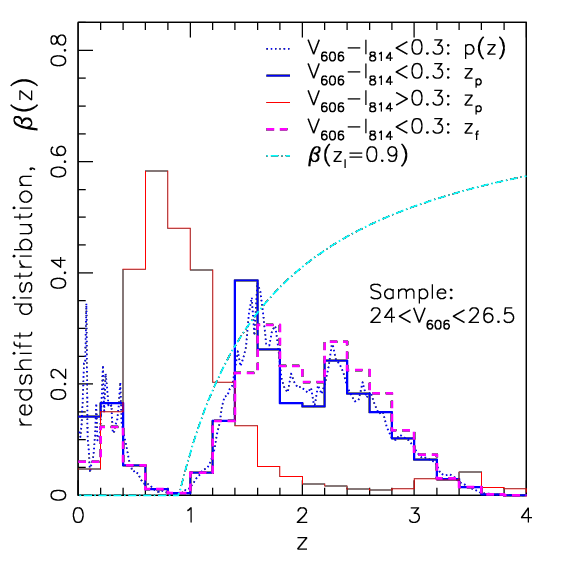
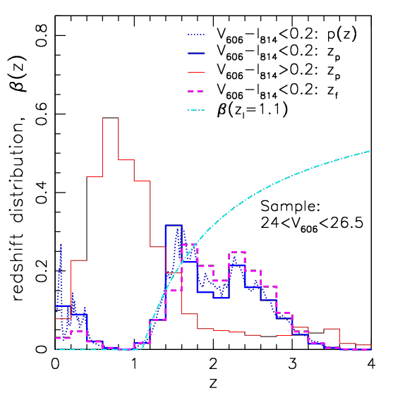


For clusters at we select source galaxies with . This maximises the background galaxy density while at the same time removing of the CANDELS galaxies at that pass the other weak lensing cuts, see the top left panel of Fig. 5. For the higher redshift clusters we apply a more stringent cut which still yields a suppression of galaxies at , at the expense of a slightly lower source density (top right panel of Fig. 5). When conducting the analysis for our cluster fields we apply slightly more conservative colour cuts that are bluer by 0.1 mag for the faintest sources in our analysis, as they show the largest photometric scatter. As a result, we obtain a similar fraction of removed galaxies at the cluster redshifts when taking photometric scatter into account (see Sect. 6.4 and Appendix D.3).
In Fig. 4 we also over-plot synthetic colours of redshifted SED templates for star forming galaxies employed in the Bayesian Photometric Redshift (BPZ) algorithm (Benítez, 2000). This includes the SB3 and SB2 star burst templates from Kinney et al. (1996) as recalibrated by Benítez et al. (2004). We additionally include a young star burst model (SSP 25Myr), which is one of the templates introduced by Coe et al. (2006) into BPZ to improve photometric redshift estimates for very blue galaxies in the HUDF. The shown SED corresponds to a simple stellar population (SSP) model with an age of 25 Myr and metallicity (Bruzual & Charlot, 2003). At the cluster redshifts, the colours of the SB3 and SB2 templates approximately describe the range of colours of typical blue cloud galaxies, which are well removed by our colour selection. In contrast, while the colour of the SSP 25 Myr model appears to be representative for a considerable fraction of the background galaxies, it approximately marks the location of the most extreme blue outliers at the cluster redshifts, which are not fully removed by our colour selection scheme. If the clusters contain a substantial fraction of such extremely blue galaxies, this might introduce some residual cluster member contamination in our lensing catalogue. We investigate this issue in Appendix F, concluding that such galaxies have a negligible impact for our analysis despite the physical over-density of galaxies in clusters. We also present empirical tests for residual contamination by cluster galaxies in Sect. 6.8.
6.3 Statistical correction for systematic features in the photometric redshift distribution
We base our estimate of the source redshift distribution on the CANDELS photo- catalogues because of their high completeness at the depth of our SPT ACS observations (Sect. 6.1), allowing us to select galaxies that are representative for the galaxies used in our lensing analysis. However, it is important to realise that such photo- estimates may contain systematic features (e.g. catastrophic outliers) that can bias the inferred redshift distribution and accordingly the lensing results. As an example, the cosmological weak lensing analysis of COSMOS data by S10 suggests that the majority of faint galaxies in the COSMOS-30 photometric redshift catalogue (Ilbert et al., 2009) that have a primary peak in their posterior redshift probability distribution at low redshifts but also a secondary peak at high redshifts, are truly at high redshift. Likewise, the galaxy-galaxy lensing analysis of CFHTLenS data by Heymans et al. (2012) indicates that a significant fraction of galaxies with an assigned photometric redshift are truly at high redshift. In the following subsections we exploit additional data sets to check the accuracy of the CANDELS photo-s and implement a statistical correction for relevant systematic features.
6.3.1 Tests and statistical correction based on HUDF data
The Hubble Ultra Deep Field (HUDF) is located within one of the CANDELS fields (GOODS-South). The very deep multi-wavelength observations conducted in the HUDF can therefore be used for cross-checks of the CANDELS photo-s.
As first data set we use a combination of high-fidelity spectroscopic redshifts (“spec-s”, ) compiled by Rafelski et al. (2015)555Rafelski et al. (2015) note that the object 10157 in their catalogue is problematic as it consists of a blend of two galaxies at different redshifts. We therefore exclude it from the spec-/grism- sample used in our analysis., and redshift estimates extracted by the 3D-HST team (Brammer et al., 2012, 2013) from the combination of deep HST WFC3/IR slitless grism spectroscopy and very deep HST optical/NIR imaging. These “grism-s” () significantly enlarge the sample of high- () galaxies with high quality redshift estimates, where typical errors of the grism-s are (Brammer et al., 2012; Momcheva et al., 2016).
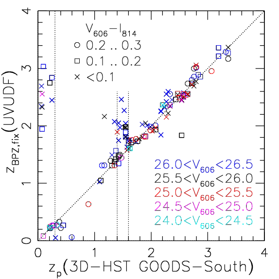
We compare the CANDELS photo-s to the HUDF estimates in the left panel of Fig. 6. The majority of the data points closely follow the diagonal, suggesting that the 3D-HST photo-s are overall well calibrated as needed for unbiased estimates of the redshift distribution. However, we note the presence of two relevant systematic features: first, there are three catastrophic outliers that are at high , but are assigned a low . Second, there is an increased, asymmetric scatter at . Most notably, many galaxies with an assigned photometric redshift are actually at higher redshift. This is likely the result of redshift focusing effects (e.g. Wolf, 2009) caused by the broad band HST filters. While this comparison allows us to identify these issues, the matched catalogue is insufficient to derive a robust statistical correction for our full photometric sample given the incompleteness of the sample.
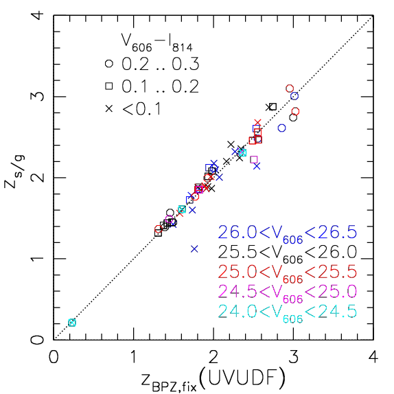
To overcome this limitation of incompleteness, we use deep photometric redshifts computed by Rafelski et al. (2015) using HUDF data as a second comparison sample. Compared to the CANDELS photo-s they benefit from much deeper HST optical (Beckwith et al., 2006) and NIR imaging (Koekemoer et al., 2013), and additionally incorporate new HST/UVIS Near UV imaging from the UVUDF project (Teplitz et al., 2013) taken in the F225W, F275W, and F336W filters. These bands probe the Lyman break in the redshift range , which contains most of our weak lensing source galaxies. At these redshifts, the NIR imaging additionally probes the location of the Balmer/4000Å break. Hence, we expect that the resulting photo- should be highly robust against catastrophic outliers. We test this by comparing them to the redshifts in the middle panel of Fig. 6. Here we use the photo- estimates obtained by Rafelski et al. (2015) using BPZ as it yields the highest robustness against catastrophic outliers in their analysis. Note that the comparison of and suggests that slightly overestimates the redshifts for the colour-selected sample in the redshift intervals and , with median redshift offsets of 0.071 and 0.171, respectively. We have therefore subtracted these offsets in the corresponding redshift intervals, yielding , which is shown in Fig. 6. As visible in the middle panel of Fig. 6, correlates tightly with . In particular, the three catastrophic outliers from the left panel are now correctly placed at high redshifts. Likewise, the redshift focusing effects are basically removed. The remaining scatter with one moderate outlier has negligible impact on our results. For example, agrees to 0.4% between and for the matched catalogue and clusters at (we include this in the systematic error budget of Sect. 6.3.2). This suggests that provides a sufficiently accurate approximation for the true redshift. Hence, we use as a reference to obtain a statistical correction for the systematic features of the CANDELS photo-s.
We compare the 3D-HST photo-s in the HUDF to in the right panel of Fig. 6, again showing the previously identified catastrophic outliers at and redshift focusing effects at , but now at the full depth of our photometric sample. The catastrophic outliers with are dominated by blue galaxies, for which 9 out of 12 galaxies appear to be truly at high redshifts. In order to implement a statistical correction for these outliers for the full CANDELS catalogue, we note the 12 redshift offsets . We bootstrap this empirically defined distribution to define the correction: for each CANDELS galaxy with and we add a randomly drawn offset to its . Likewise, we apply a statistical correction for the redshift focusing within the redshift range for galaxies with (which are most strongly affected, see Fig. 6), again randomly sampling from the corresponding offsets in the HUDF. For the latter correction we split the galaxies into two magnitude ranges ( and ) given that the fainter galaxies appear to suffer from the redshift focusing effects more strongly. We show the resulting distribution of statistically corrected redshifts as magenta dashed histograms in the top panels of Fig. 5. As expected, it has a lower fraction of low- galaxies compared to the uncorrected distribution, as well as a reduction of the redshift focusing peak at . Both effects are compensated by a higher fraction of high- galaxies, where we also note that the local minimum at , which likely results from the redshift focusing (see also Sect. 6.3.3), is reduced.
Averaged over our full cluster sample, and accounting for the magnitude-dependent effects explained in the following sections (e.g. shape weights), the application of this correction scheme leads to a 12% decrease of the resulting cluster masses. Of this, 10% originate from the correction for catastrophic outliers, and 2% from the correction for redshift focusing.
6.3.2 Uncertainty of the statistical correction of the redshift distribution
The statistical correction of the redshift distribution explained in Sect. 6.3.1 has a non-negligible impact on our analysis. Therefore it is important to quantify its uncertainty. We consider a number of effects that affect the uncertainty: first, we estimate the statistical uncertainty originating from the limited size of the HUDF catalogue by generating bootstrapped versions of it, which are then used to generate the offset samples. This yields a small, 0.5% uncertainty regarding the average masses. Second, our correction scheme assumes that the relative effects seen in the HUDF are representative for the full CANDELS area. However, some previous studies suggest that the GOODS-South field, which contains the HUDF, could be somewhat under-dense at lower redshifts compared to the cosmic mean (e.g. Schrabback et al., 2007; Hartlap et al., 2009). To obtain a worst case estimate of the impact this could have, we assume that the GOODS-South field could be under-dense at low redshifts by a factor 3 compared to the cosmic mean. Hence, we artificially boost the number of HUDF galaxies with that are truly at low- by a factor 3 for the generation of the offset pool. On average this leads to a 3% increase of the cluster masses. Third, we note that our correction for redshift focusing incorporates most but not all of the corresponding outliers in the right panel of Fig. 6. We assume a conservative 50% relative uncertainty on the 2% correction, corresponding to an absolute 1% uncertainty. Adding all individual systematic uncertainties identified here and in Sect. 6.3.1 in quadrature yields a combined systematic uncertainty for the systematic corrections to the photometric redshifts of 3.3% in the average cluster mass.
6.3.3 Consistency checks using spectroscopic and grism redshifts in the CANDELS fields
In Sect. 6.3.1 we obtained a statistical correction for systematic features in the CANDELS photo-s using very deep data available in the HUDF. Here we present cross-checks for this correction using the CANDELS redshift catalogue from Momcheva et al. (2016), which combines a compilation of high fidelity spectroscopic redshifts from S14 with redshift estimates derived from their joint analysis of slitless WFC3/NIR grism spectra from the 3D-HST project and the S14 photometric catalogues. These grism data are shallower than those available in the HUDF (see Sect. 6.3.1) but cover a much wider area. We restrict the use of these grism-s to relatively bright galaxies (NIR magnitude ). These galaxies were individually inspected by the 3D-HST team, allowing us to select galaxies classified to have robust redshift estimates. For these relatively bright galaxies the continuum emission is comfortably detected in the grism data, yielding high-quality redshift estimates with a typical redshift error of (Momcheva et al., 2016), which we can neglect compared to the photo- uncertainties.
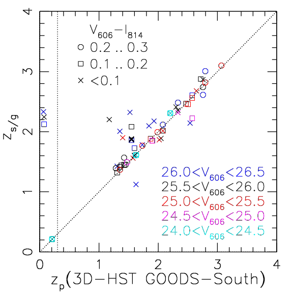
For the combined sample of galaxies with spec-s and grism-s we compare the colour-selected histogram of spec-s/grism-s (, using in case both are available) to the histogram of their photo-s in the bottom panels of Fig. 5. Here we note two points: First, the spec-s/grism-s confirm that the colour selection indeed provides a very efficient removal of galaxies at our targeted cluster redshifts. Second, the high- galaxies are distributed in a relatively symmetric, unimodal peak that has a maximum at according to spec-s/grism-s. In contrast, the photo- histogram shows two slight peaks ( and ). This is consistent with the conclusion from Sect. 6.3.1 that the peaks in the photo- histogram of the full photometric sample (top panels of Fig. 5) at these redshifts are a result of redshift focusing effects and not true large-scale structure peaks in the galaxy distribution.
As a further cross-check we reconstruct the redshift distribution of the photometric sample by exploiting its spatial cross-correlation with the spec-s/grism- sample, applying the technique developed by Newman (2008); Schmidt et al. (2013); Ménard et al. (2013). Specifically, we use the implementation in The-wiZZ666Available at https://github.com/morriscb/The-wiZZ redshift recovery code (Morrison et al., 2017). We provide the details of this analysis in Appendix C, showing that it independently confirms the presence of the catastrophic redshift outliers and redshift focusing effects.
6.3.4 Limitations of the averaged posterior probability distribution
Past weak lensing studies suggest that a better approximation of the true source redshift distribution may be given by the average photometric redshift posterior probability distribution of all sources compared to a histogram of the best-fit (or peak) photometric redshifts (see e.g. Heymans et al., 2012; Benjamin et al., 2013; Bonnett, 2015). To test this we recompute the using EAZY from the S14 photometric catalogues, which is necessary as the are not reported in the S14 catalogues.
As visible in Fig. 5, the redshift distribution inferred from the averaged is relatively similar to the normalised histogram of the peak photometric redshifts . We note that the redshift focusing peak at and local minimum at are slightly less pronounced in the averaged , but they do not reach the level suggested by the corrected histogram. More severely, the averaged over predicts the fraction of low- galaxies compared to the distribution similarly to the histogram. We therefore conclude that the use of the averaged instead of the histogram is insufficient to account for the systematic features identified in Sect. 6.3.1.
6.4 Source selection in the presence of photometric scatter
Outside the area of the central F814W ACS tile we only have single band F606W observations from HST. For the colour selection we therefore have to combine the F606W data with the VLT/FORS2 -band imaging (see Sect. 4.2). We measure colours between these images as described in Appendix D.1. However, VLT/FORS2 -band observations are not available in all CANDELS fields. We therefore need to accurately map the selection in the ACS+FORS2-based colour to the colour available in CANDELS. We empirically obtain this mapping through the comparison of both colour estimates in the inner cluster regions, where both are available (see Appendix D.2).
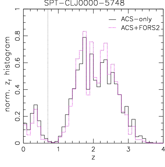
As described in Appendix D.3 we add photometric scatter to the catalogues from the CANDELS fields to mimic the noise properties of the cluster fields for the colour selection. In particular, we apply an empirical model for the (non-Gaussian) scatter between the ACS-only and the ACS+FORS2 colours derived from the comparison of the colour measurements in the inner cluster regions. The ACS-only colour selection has higher signal-to-noise, allowing us to include galaxies with in the analysis. In contrast, the ACS+FORS2 colour selection is more noisy, which is why we have to employ shallower magnitude limits (dependent on the depth of the VLT data, see Table 2) and more stringent colour cuts (see Table 11 in Appendix D). Fig. 7 demonstrates that this approach leads to a robust removal of galaxies at the cluster redshift despite the presence of noise. Here we show the histogram of the statistically corrected redshift estimates for the CANDELS galaxies passing the colour selection for SPT-CL 00005748 after application of the photometric scatter. Averaged over the cluster sample we find that 98.9% (98.1%) of the CANDELS galaxies with are removed by the ACS+FORS2 (ACS-only) colour selection scheme when the noise is taken into account. As shown in Appendix F this translates into a negligible expected cluster member contamination in the weak lensing analysis. In addition, we will show in Sect. 6.8 that the total source density and the source density profiles provide limits on the residual cluster member contamination, which are consistent with no contamination.
6.5 Analysis in magnitude bins
As shown in Fig. 8, increases moderately within the magnitude range , which is due to a larger fraction of high-redshift galaxies passing the colour selection at fainter magnitudes. We only include galaxies with in our analysis as brighter galaxies contain only a low fraction of background sources. We split the source galaxies into subsets according to magnitude (0.5 mag-wide bins) in order to optimise the of our measurement. This allows us to adequately weight the bins in the analysis not only accounting for the shape weight , but also the geometric lensing efficiency.
6.6 Accounting for line-of-sight variations
There is statistical uncertainty on how well we can estimate the cosmic mean in a magnitude bin (given our lensing and colour selection) due to sampling variance and the finite sky-coverage of CANDELS. Furthermore, the actual redshift distribution along the line-of-sight to each of our clusters will be randomly sampled from this cosmic mean distribution, leading to additional statistical scatter, see e.g. Hoekstra et al. (2011b), who show that this is particularly relevant for high- clusters.
To account for the statistical scatter in our weak lensing mass analysis (Sect. 7), we subdivide the CANDELS fields into sub-patches that match the size of our cluster field observations (single ACS tiles for the ACS-only colour selection and mosaics for the ACS+FORS2 selection) and compute and from the redshift distribution of each sub-patch . From the scatter of these quantities between all sub-patches we compute the resulting scatter in the mass constraints in Sect. 7.2.
Furthermore, we need to investigate if the uncertainty on the estimate of the cosmic mean due to the finite sky-coverage of CANDELS adds a significant systematic uncertainty in our error-budget. For this, we first compute the uncertainty on the mean from the variance of the . Assuming all sub-patches were statistically independent, we find a very small relative uncertainty () for our lowest-redshift cluster SPT-CL J23315051 at and () for our highest-redshift cluster SPT-CL J21065844 at using the ACS-only (ACS+FORS2) colour selection combining all magnitude bins. However, due to large-scale structure the within each CANDELS field will be correlated. A more conservative estimate can be obtained by computing for each CANDELS field (without sub-patches) and estimating from the variation between the five fields777Here we want to investigate how well we can estimate the cosmic mean redshift distribution from CANDELS, for which sub-patches are not needed. The sub-patches are needed to estimate the line-of-sight scatter in between the different cluster fields, as discussed in the second paragraph of this subsection.. This yields (0.6%) for SPT-CL J23315051 and () for SPT-CL J21065844, again employing the ACS-only (ACS+FORS2) colour selection. This uncertainty is taken into account in our systematic error budget in Sect. 7.5, but we note that it is very small compared to our statistical errors in all cases.
6.7 Accounting for magnification
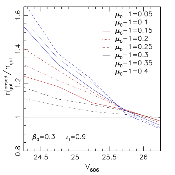
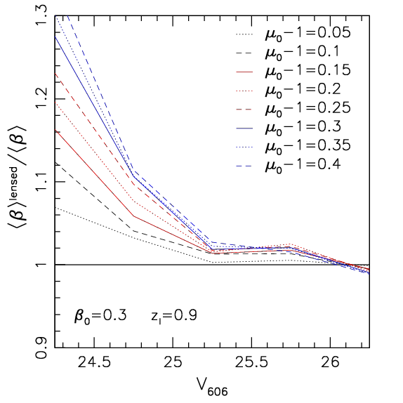
In addition to the shear, the weak lensing effect of the clusters magnifies background sources by a factor given by Eq. (15). This effectively alters the source redshift distribution, but this effect has typically been ignored in previous studies. For our analysis this has three effects: first, it increases the fluxes of sources by a factor , which may place them into brighter magnitude bins, thus increasing the total source density by including galaxies which are intrinsically too faint to be included. Second, it reduces the source sky area we observe, diluting the number density of sources by a factor . Finally, the magnification of object sizes may lead to the inclusion of some small galaxies which would otherwise be excluded by the lensing size cut. However, the large majority of our galaxies are well-resolved with HST, so we will ignore this latter effect (but it may be more relevant for data with lower image quality).
We estimate the impact of the first and second effect from a colour-selected888Here we account for the magnitude-dependence of our colour cut (see Table 11 in Appendix D), by basing it on the lensed magnitude. S14 CANDELS catalogue (lensing is achromatic). Here we restrict the analysis to the deeper GOODS fields, initially including galaxies down to . For this part of the analysis we do not require a matching entry in our 1 orbit-depth shape catalogue in order to maximise the completeness at the faint end. We include the statistical correction for catastrophic redshift outliers and redshift focusing from Sect. 6.3.1, where we apply the same scheme also for one additional magnitude bin with . For each cluster redshift we compute for each galaxy (using ) in the CANDELS catalogue and approximate the magnification as
| (23) |
where indicates the magnification at an arbitrary fiducial , for which we use close to the mean for our higher redshift clusters (compare Table 3). The scaling in Eq. (23) is adequate in the weak lensing limit (, ), in which case Eq. (15) simplifies to
| (24) |
where and are the convergence and shear for . In practice we find that the assumed linear scaling with in Eq. (23) is sufficiently accurate for all of our clusters within the considered radial range of the tangential reduced shear profile fits (see Sect. 7.2).
| Cluster | |||||
|---|---|---|---|---|---|
| ACS-only | ACS+FORS2 | ||||
| SPT-CL 00005748 | 0.466 | 0.243 | 0.053 | 18.2 | 7.2 |
| SPT-CL 01024915 | 0.374 | 0.163 | 0.068 | 20.4 | 3.6 |
| SPT-CL 05335005 | 0.368 | 0.159 | 0.062 | 19.7 | 5.4 |
| SPT-CL 05465345 | 0.303 | 0.107 | 0.083 | 13.1 | 2.9 |
| SPT-CL 05595249 | 0.505 | 0.288 | 0.064 | 18.2 | 4.0 |
| SPT-CL 06155746 | 0.334 | 0.132 | 0.075 | 18.0 | 2.3 |
| SPT-CL 20405725 | 0.344 | 0.141 | 0.077 | 16.2 | 3.5 |
| SPT-CL 21065844 | 0.282 | 0.093 | 0.087 | 9.2 | 2.0 |
| SPT-CL 23315051 | 0.522 | 0.308 | 0.059 | 16.2 | 8.3 |
| SPT-CL 23375942 | 0.425 | 0.205 | 0.059 | 18.3 | 7.6 |
| SPT-CL 23415119 | 0.320 | 0.122 | 0.067 | 19.1 | 9.3 |
| SPT-CL 23425411 | 0.300 | 0.105 | 0.082 | 15.8 | 2.5 |
| SPT-CL 23595009 | 0.423 | 0.204 | 0.055 | 16.6 | 8.7 |
Note. — Column 1: Cluster designation. Columns 2–4: , , and averaged over both colour selection schemes and all magnitude bins that are included in the NFW fits according to their corresponding shape weight sum. Columns 5–6: Density of selected sources in the cluster fields for the ACS-only and the ACS+FORS2 colour selection schemes, respectively.
For each galaxy in the CANDELS catalogue we compute for a range of . We then estimate the magnified magnitude for each galaxy, and keep track of the reduced sky area through a weight . By binning in we then compute the lensed number density
| (25) |
and the mean lensed geometric lensing efficiency
| (26) |
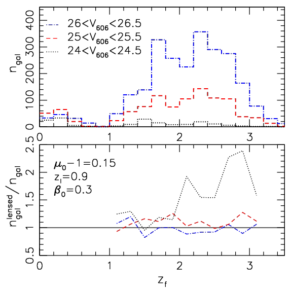
where the summations are over all galaxies with lensed magnitudes falling into the corresponding bin. In Fig. 9 we plot the ratio of these quantities to their not-lensed counterparts and computed in bins with uniform weight999When computing the relative impact of magnification on the number density and mean lensing efficiency we deliberately do not include the shape weights, as we would otherwise need to account for the increase in and thus due to the magnification. Since we perform the full analysis in magnitude bins, with very little variation in within a bin, our approach constitutes a very good approximation. . This shows that magnification has only a minor net effect at magnitudes –, which contain a large fraction of our source galaxies. In contrast, it significantly boosts both quantities for brighter magnitudes . The net impact of magnification on high- cluster mass estimates therefore strongly depends on the depth of the observations. For illustration we also show the redshift distributions within three magnitude bins and their relative change after applying magnification with and in Fig. 10.
Previous weak lensing magnification studies have made the simplifying assumptions that sources are located at a single redshift and that the source counts can be described as a power law. Under these assumptions the ratio of the lensed and non-lensed cumulative source densities above a magnitude
| (27) |
depends only on the magnification and the slope of the logarithmic cumulative number counts
| (28) |
(e.g. Broadhurst, Taylor & Peacock, 1995; Chiu et al., 2016a), where slopes () lead to a net increase (decrease) of the counts. As an illustration we estimate from our colour () and shape-selected GOODS-South and GOODS-North catalogue, finding that it can approximately be described as
| (29) |
for . Under these simplifying assumptions we therefore expect a significant boost in the source density at bright magnitudes (–) where the slope of the number counts is steep, and only a small boost towards fainter magnitudes (), where the slope of the number counts is shallower. This roughly agrees with the more accurate results shown in Fig. 9, but there are noticeable differences, such as the slight net decrease in the source density at in Fig. 9. As our sources are not at a single redshift, the simplifying assumptions are clearly not met, which is why we base our analysis on the more accurate approach described above.
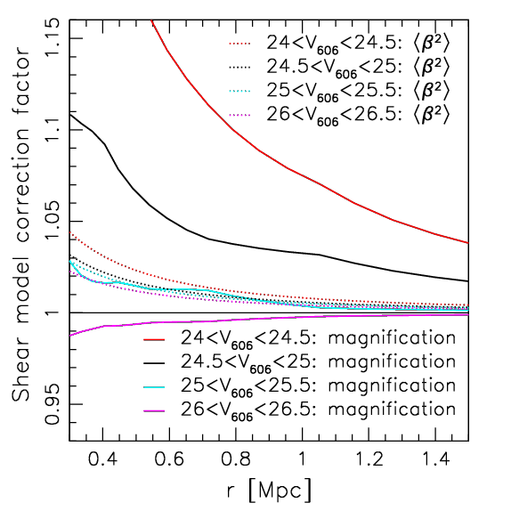
When fitting the reduced cluster shear profiles with NFW models in Sect. 7, we compute a profile for magnitude bin and a given mass from the NFW model predictions for both and according to Eq. (15). Employing Eq. (23) with we compute the corresponding profile and obtain radius-dependent corrections and by interpolating our CANDELS-based estimates (Fig. 9) between the discrete values. The fact that we compute the magnification in the NFW prediction from both and is our primary motivation to conduct the interpolation in terms of and not . This provides a more accurate correction than if the shear contribution is ignored, even though we assume the linear scaling in in Eq. (23) to simplify the CANDELS analysis.
On average the application of the correction for magnification-induced changes in the redshift distribution reduces our estimated cluster masses by 3%. This net impact is relatively small since the majority of our sources are at , requiring small corrections. Also, we exclude the cluster cores, where the correction is the largest (see Fig. 11), from our tangential shear profile fits (see Sect. 7). However, we emphasise that weak lensing studies of high- clusters using shallower data will be affected more strongly and should adequately model this effect.
We note a subtle limitation of our modelling approach for magnification which results from our choice to conduct the analysis as function of aperture magnitude. Here we ignore the fact that the increase in size due to magnification will lead to a larger fraction of the flux being outside the fixed aperture radius than without magnification. As a test we also conducted the magnification analysis using aperture-corrected magnitudes from CANDELS101010The 3D-HST CANDELS catalogue provides aperture magnitudes, which we can directly compare to our measurements, plus an aperture correction based on the -band, which is however not available for our cluster fields., finding similar models as in Fig. 9 but shifted to brighter magnitudes, with reaching unity at –. Given the very minor impact magnification has for our data compared to the statistical uncertainties, the described subtle limitation can safely be ignored for the current study. In the future this can be avoided by computing aperture corrections in the filter used for shape measurements both for CANDELS and the cluster fields.
6.8 Number density consistency tests
The measurements of the total source density and its radial dependence can be used to test the cluster member removal and our procedure to consistently select galaxies in the cluster and CANDELS fields in the presence of noise (Sect. 6.4). When computing the source density we account for masks and apply an approximate correction111111Here we approximate the sky area blocked by a galaxy through the parameter from Source Extractor. Hoekstra et al. (2015) present a more detailed treatment using image simulations, finding that obscuration by cluster members is a relatively minor effect for their analysis. Our cluster galaxies are at higher redshift and are thus more strongly dimmed, leading to an even smaller impact of obscuration by cluster members. Our pipeline automatically masks the image region around bright and very extended galaxies. With this applied we find that accounting for the sky area blocked by unmasked brighter galaxies via the parameter leads to per cent changes in the source density even for the faintest galaxies considered in our analysis. for the impact of obscuration by cluster members (Simet & Mandelbaum, 2015). We also account for the impact of cluster magnification, employing the corresponding radius-dependent magnification model for each cluster from Sect. 6.7.
6.8.1 Total source density
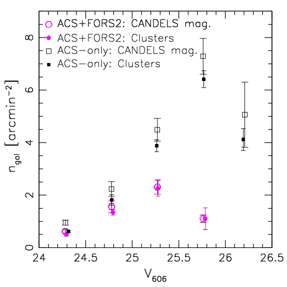
In Fig. 12 we compare the average density of selected source galaxies in the cluster fields as function of to the corresponding average density in the CANDELS fields corrected for the expected influence of magnification given our best-fit NFW cluster mass models. There is very good agreement for the ACS+FORS2 selection and reasonable agreement for the ACS-only selection (error-bars are correlated because of large-scale structure). Fig. 12 also visualises that the ACS-only analysis (with two ACS bands) provides a substantially higher average total density of selected sources in the cluster fields of 16.8 galaxies/arcmin2 compared to 5.2 galaxies/arcmin2 for the ACS+FORS2 colour selection (see Table 3 for the total source densities in each field). This shows that either substantially deeper ground-based imaging or ACS-based colours for the full imaging area would be required for the colour selection in order to adequately exploit the full depth of the ACS shape catalogues.
6.8.2 Source density profile
As an additional cross-check for the removal of cluster galaxies and our magnification model we plot the radial source density profiles for the ACS-only and ACS+FORS2 selected samples in Fig. 13, averaged over all clusters, as function of cluster-centric distance from the X-ray centre (nearly identical results are obtained when using the SZ peak location, see Sect. 7) in units of their corresponding as estimated from the SZ signal. Here we compare the case with and without applying the magnification correction. The difference is small given that the magnification is relatively weak for the majority of the clusters. Also, most of the source galaxies have faint magnitudes, where the net impact of magnification is small (see Fig. 9). The net difference is strongest for the inner cluster regions where the magnification is strongest.
In the case of a complete cluster galaxy removal and an accurate correction for magnification we expect to measure a number density that is consistent with being flat as function of radius. To test this, we perform a model comparison test using the cluster sample-averaged number density profiles, assuming that errors were independent and Gaussian distributed. Each radial bin used in the test is the average of at least three clusters, while uncertainties are determined by bootstrapping the cluster sample. With these measures, the statistic should be a crude yet useful approximation to the true uncertainty distribution, while allowing us to use analytic model quality of fit and comparison tests.
As expected for adequate removal of cluster members and magnification correction, we find that the source density profiles are consistent with being flat. For the ACS-only case, the maximum likelihood constant number density model returns a with 4 degrees of freedom, while a inverse-r profile with two parameters, the contamination fraction at and the background number density (Hoekstra, 2007), returns a with 3 degrees of freedom. Both are acceptable models at , where the improvement in is consistent with random according to an F-test (). The rather low values might be due to our assumption of independent errors between bins, which neglects the effects of large-scale structure. For the ACS+FORS2 selection, the constant number density model returns with 8 degrees of freedom, while an exponential model (see Appendix E and Applegate et al., 2014), which is preferred over the inverse-r model in this case, returns with 7 degrees of freedom, again suggesting that a flat number density model is sufficient ( from the F-test). For a general test for the consistency of the combined number density profile being flat we allow for negative in these fits, which could for example be mimicked by an incorrect magnification correction. The maximum likelihood parameter value for the inverse-r contamination model fit to the ACS-only number density profile indeed peaks at slightly, but not significantly negative values, . Fig. 13 shows the measured number density profiles and maximum-likelihood model fits for both selections.
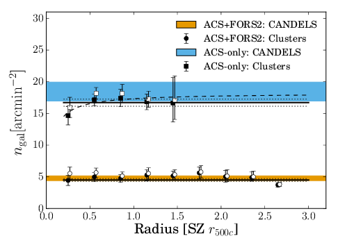
7 Weak lensing constraints and mass analysis
We reconstruct the projected mass distribution in our cluster fields in Sect. 7.1 and constrain the cluster masses via fits to the tangential reduced shear profile in Sect. 7.2. In Sect. 7.3 we compare the stacked shear profiles from all clusters for the different centres used in the analysis and investigate the consistency of the data with different concentration–mass relations. In Sect. 7.4 we detail on the simulations used to calibrate the mass estimates. We discuss the systematic error budget in Sect. 7.5.
7.1 Mass maps
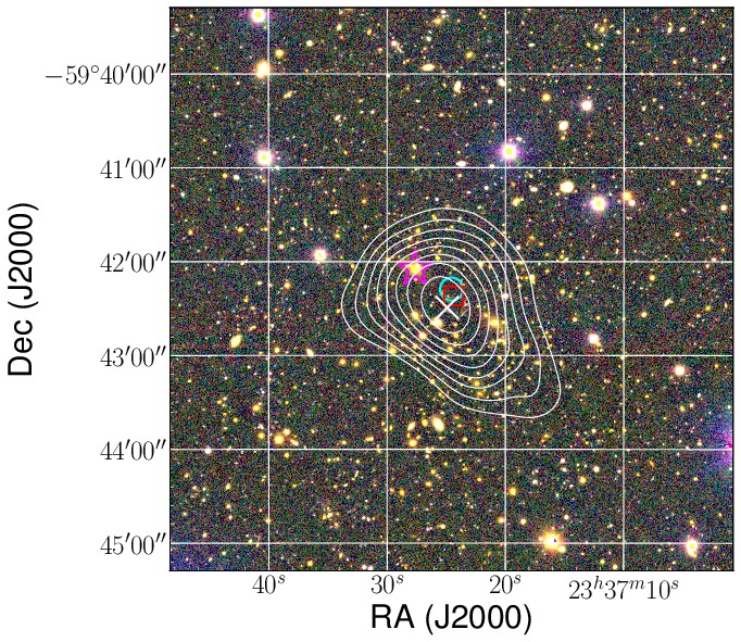
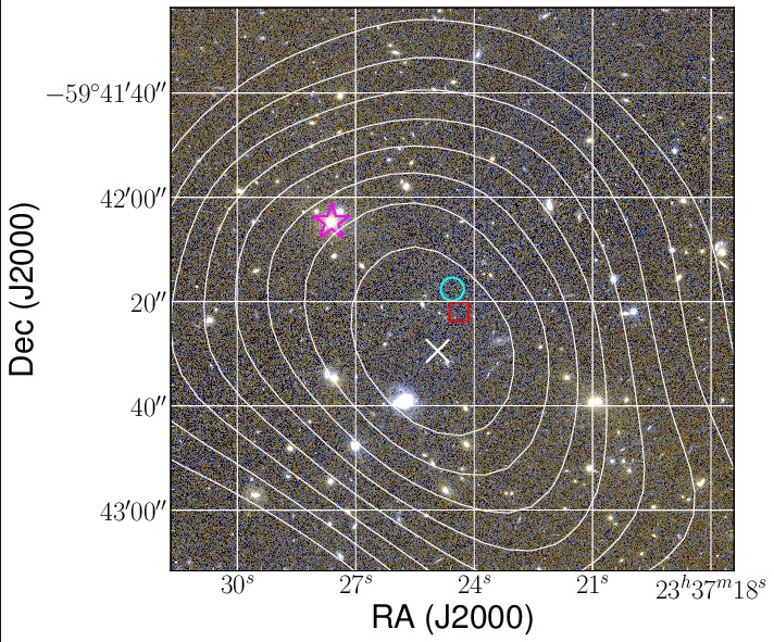
The weak lensing shear and convergence are linked as they are both based on second-order derivatives of the lensing potential. Therefore, a reconstruction of the convergence field can be obtained from the shear field up to a constant (Kaiser & Squires, 1993), which is the mass-sheet degeneracy (Schneider & Seitz, 1995). Motivated by the different colour-selected source densities in the inner and outer regions of our clusters we employ a Wiener filter for the convergence reconstruction using an implementation described in McInnes et al. (2009) and Simon, Taylor & Hartlap (2009). This code estimates the convergence on a grid taking the spatial variation in the source number density into account; it applies more smoothing where the number density of sources is lower. The smoothing in the Wiener filtered map employs the shear two-point correlation function (e.g. Schneider, 2006) as a prior on the angular correlation of the convergence, which affects the degree of smoothing. For this, we measure in the cluster fields and find that it is on average approximately described by the fitting function . We fix the mass-sheet degeneracy by setting the average convergence inside each cluster field to zero. While this underestimates the overall convergence for our relatively small cluster fields, this is irrelevant as we use the reconstructions to study positional offsets and the signal-to-noise () ratio of relative mass distributions, but not to obtain quantitative mass constraints. To compute the mass maps we generate 500 noise maps for each cluster by randomising the ellipticity phases and repeating the mass reconstruction. We then define the mass map as the ratio of the reconstruction from the actual data and the r.m.s. image of the noise reconstructions.
| Cluster | |||||||
|---|---|---|---|---|---|---|---|
| [deg J2000] | [deg J2000] | [arcsec] | [arcsec] | [kpc] | [kpc] | ||
| SPT-CL 00005748 | 0.25195 | 1.9 | 2.2 | 14 | 16 | 5.7 | |
| SPT-CL 01024915 | 15.71743 | 7.1 | 7.9 | 55 | 61 | 5.7 | |
| SPT-CL 05335005 | 83.39772 | 10.2 | 8.0 | 79 | 62 | 3.0 | |
| SPT-CL 05465345 | 86.65396 | 5.1 | 3.7 | 41 | 30 | 3.6 | |
| SPT-CL 05595249 | 89.92875 | 4.3 | 3.6 | 29 | 24 | 5.0 | |
| SPT-CL 06155746 | 93.96562 | 4.3 | 2.8 | 34 | 23 | 5.1 | |
| SPT-CL 20405725 | 310.06389 | 5.0 | 5.1 | 40 | 40 | 3.1 | |
| SPT-CL 21065844 | 316.52210 | 7.2 | 4.5 | 59 | 37 | 2.9 | |
| SPT-CL 23315051 | 352.96521 | 1.8 | 2.3 | 12 | 15 | 5.1 | |
| SPT-CL 23375942 | 354.35384 | 1.8 | 2.5 | 13 | 19 | 6.0 | |
| SPT-CL 23415119 | 355.30057 | 5.3 | 5.4 | 42 | 44 | 3.3 | |
| SPT-CL 23425411 | 355.69305 | 3.7 | 9.9 | 30 | 80 | 3.1 | |
| SPT-CL 23595009 | 359.93213 | 4.7 | 4.8 | 35 | 35 | 5.2 |
As an example, Fig. 14 shows an overlay of the contours of the mass reconstruction (starting at in steps of ) for SPT-CL 23375942 on a FORS2 colour image (left) as well as a cut-out of the ACS imaging (right). Here we also indicate the locations of the X-ray centroid, BCG, and SZ peak (see Table 1). The corresponding figures for the other clusters are shown in Appendix G.
For all clusters the weak lensing reconstruction shows a mass peak associated with the cluster, with a peak signal-to-noise ratio between and . Typically, the mass reconstructions follow the distribution of red cluster galaxies well, especially for the clusters with . Of these clusters, SPT-CL 00005748 and SPT-CL 23315051 show relatively symmetric mass reconstructions consistent with more relaxed morphologies, while SPT-CL 01024915, SPT-CL 05595249, SPT-CL 06155746, SPT-CL 23375942, and SPT-CL 23595009 show more elongated or perturbed morphologies. In particular, SPT-CL 01024915 is known to be an extreme merger (Menanteau et al., 2012), for which our mass reconstruction separates both main components well (see also the independent weak lensing analysis by Jee et al., 2014).
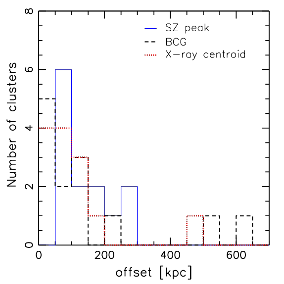
In the mass signal-to-noise maps we determine the position of the mass peak of the corresponding cluster by identifying the pixel with the highest within 90′′ from the SZ peak location. We report these positions in Table 4 along with estimates of their uncertainty and peak signal-to-noise . The positional uncertainties are estimated by generating 500 bootstrap samples of the source catalogue for which we repeat the reconstruction and identification of the peak location. The average r.m.s. positional uncertainty (including both directions) for the full sample is 59 kpc.
Dietrich et al. (2012) investigate the origin of offsets between peaks in weak lensing mass reconstructions and the projected position of the 3D centre (defined as the minimum of the potential) of cluster-scale dark matter haloes in the Millennium Simulation (Springel et al., 2005; Hilbert et al., 2009). Without shape noise and smoothing applied in the mass reconstruction they find very small offsets: their analysis using sources at is most similar to the set-up of our study, yielding a 90th percentile offset of kpc. Hence, projection effects and large-scale structure have a negligible impact for the measured offsets in typical observing scenarios. Dietrich et al. (2012) find that smoothing and shape noise increase the offsets substantially, where the addition of shape noise has the biggest impact unless unnecessarily large smoothing kernels are used. Our bootstrap analysis provides an estimate for the positional uncertainty due to shape noise. However, the analysis likely underestimates the true positional uncertainty with respect to the 3D cluster centre as it does not explicitly account for the impact of smoothing. Nevertheless, we can use the distribution of offsets between the peaks in the mass signal-to-noise maps and different proxies for the cluster centre, namely the X-ray centroid, SZ peak, and BCG position, to test if these are similarly good proxies for the true 3D cluster centre position. Fig. 15 shows a histogram of the corresponding offset distributions. We also summarise the average, r.m.s., and median of these offset distributions in Table 5, where errors indicate the dispersion of the corresponding values when bootstrapping the cluster sample. While the X-ray centroids yield the smallest average and median offsets, their r.m.s. offset is similar to the one for the SZ peaks. The distribution of offsets between the BCG locations and the mass signal-to-noise peaks has the largest r.m.s. offset, resulting from two outliers: the largest offset occurs for the merger SPT-CL 01024915 (642 kpc), where the BCG is located in the South-Eastern component while the highest signal-to-noise peak in the mass reconstruction coincides with the North-Western cluster component, which also shows a strong concentration of galaxies but has a less bright BCG (see Fig. 29). In contrast, both the SZ peak and the X-ray centroid are located between the two cluster cores and peaks of the mass reconstruction, resulting in smaller offsets. SPT-CL 05335005 also shows a large (522 kpc) offset between the BCG and the mass signal-to-noise peak, while the latter is broadly consistent with the SZ peak, X-ray centroid, and strongest galaxy concentration. This could also be explained with a merger scenario, where a smaller component hosting a brighter BCG is falling into the main cluster.
| Centre | average | r.m.s. | median |
|---|---|---|---|
| SZ peak | |||
| X-ray centroid | |||
| BCG location |
Note. — Errors indicate the dispersion of the values when bootstrapping the cluster sample.
7.2 Individual shear profile analysis
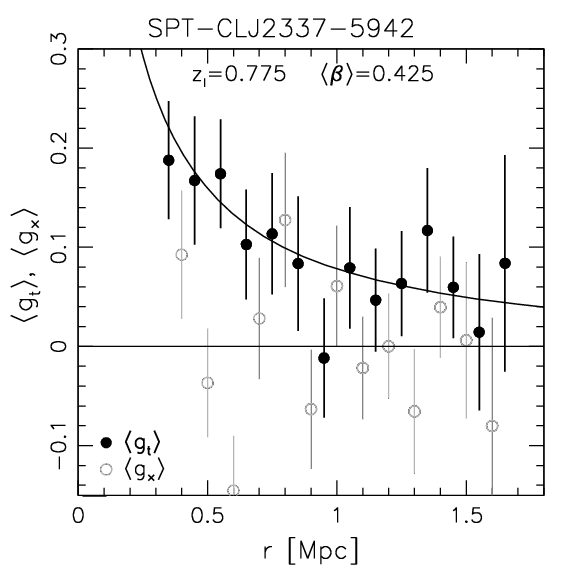
We compute profiles of the tangential reduced shear (Eq. 7) around the cluster centres in 14 linearly-spaced bins of transverse physical separation between 300 kpc and 1.7 Mpc (100 kpc-wide bins), but note that we restrict the fit range to when deriving mass constraints. Smaller scales are more susceptible to the impact of miscentring, cluster substructure, uncertainties in the concentration–mass relation, and shear calibration, while larger scales suffer from an increasingly incomplete azimuthal coverage, where 1.5 Mpc (1.3 Mpc) equals the largest radius with full azimuthal coverage at the median (lowest) redshift of the targeted clusters. We repeat the analysis for the different proxies for the cluster centre (X-ray centroid, SZ peak, and BCG position), but regard the measurements using the X-ray centroids as our primary (default) results, given that they yield the smallest average and median offsets from the peaks in the mass signal-to-noise maps (Sect. 7.1).
We compute separate tangential reduced shear profiles for each magnitude bin and colour selection scheme, where we use the ACS-only selection in the inner cluster regions where both ACS bands are available, and the ACS+FORS2 selection in the outer cluster regions. Each magnitude bin for both colour selection schemes has a separate value for and (see Sect. 6.5, Fig. 8, and average values reported in Table 3), which we correct for magnification as a function of cluster centric distance as described in Sect. 6.7. We fit the profiles from all ACS-only magnitude bins plus those ACS+FORS2 bins that have sufficiently low photometric scatter (Sect. 6.4 and Appendix D.3.2) jointly with a reduced shear profile model (see Eq. 12) according to Wright & Brainerd (2000), assuming spherical mass distributions that follow the NFW density profile (Navarro, Frenk & White, 1997). Here we use a fixed concentration–mass () relation, where we by default employ the relation from Diemer & Kravtsov (2015), but also test the consistency of the data with other relations in Sect. 7.3. While the mass distributions in individual clusters may well deviate from an NFW profile, we account for the net impact on an ensemble of clusters in Sect. 7.4. Due to the fixed concentration–mass relation we fit a one-parameter model to each cluster. Here we perform a minimisation using as free parameter, comparing the predicted reduced shear values to the measured values in each contributing bin in radius and magnitude. Given its dominance we employ a pure shape noise covariance matrix derived from our empirical weighting scheme (see Appendix A). In the fit we also allow for , which we model by switching the sign of the tangential reduced shear profile. For the calibration of scaling relations we make use of the full likelihood distribution (see Sect. 8). In addition, we identify the maximum likelihood (minimum ) location and the points, which we report in Table 6, where conversions between over-density masses use the assumed relation. Note that the derived mass constraints are expected to be biased due to effects in the mass modelling such as miscentring, which will be addressed in Sect. 7.4.
The statistical errors in Table 6 include two additional minor noise sources. The first source is given by line-of-sight variations in the redshift distribution, which we estimate from the dispersion of the estimates from the CANDELS sub-patches (see Sect. 6.6). In Table 3 we report , which introduces an additional relative noise in the mass estimates of , where . Further statistical noise is added by projections of uncorrelated large-scale structure (Hoekstra, 2001). To estimate it we compute 500 random realisations of the cosmic shear field per cluster for our reference cosmology and the colour-selected source redshift distribution as detailed in Appendix B of Simon (2012), with the non-linear matter power spectrum estimated following Takahashi et al. (2012)121212This approach generates Gaussian random shear fields based on the matter power spectrum. Comparing the resulting scatter in cluster mass estimates, Hoekstra et al. (2011b) show that approaches using the shear power spectrum provide good approximations to more accurate estimates from a ray-tracing analysis through the Millennium Simulation (Springel et al., 2005; Hilbert et al., 2009).. We add these cosmic shear field realisations to the measured shear field in the SPT cluster fields and repeat the cluster mass analysis for each realisation. The dispersion in the best-fit mass estimates then yields an estimate for the large-scale structure noise. We find that it amounts to of the statistical errors from shape noise. Additional scatter between profile-fitted weak lensing mass estimates and halo masses defined via spherical overdensities is caused by halo triaxiality, variations in cluster density profiles, and correlated large-scale structure (e.g. Gruen et al., 2015; Umetsu et al., 2016). This scatter typically amounts to for massive clusters (Becker & Kravtsov, 2011) and is not explicitly listed in Table 6. Instead, we absorb it in the intrinsic scatter accounted for in the scaling relation analysis (see Sect. 8 and Dietrich et al. in prep.).
| X-ray centres | SZ centres | |||||||
|---|---|---|---|---|---|---|---|---|
| Cluster | ||||||||
| SPT-CL 00005748 | 0.91 | 0.88 | 0.80 | 0.82 | ||||
| SPT-CL 01024915 | 0.86 | 0.88 | 0.79 | 0.79 | ||||
| SPT-CL 05335005 | 0.88 | 0.87 | 0.80 | 0.81 | ||||
| SPT-CL 05465345 | 0.86 | 0.85 | 0.72 | 0.73 | ||||
| SPT-CL 05595249 | 0.79 | 0.81 | 0.84 | 0.85 | ||||
| SPT-CL 06155746 | 0.88 | 0.85 | 0.82 | 0.80 | ||||
| SPT-CL 20405726 | 0.87 | 0.81 | 0.80 | 0.80 | ||||
| SPT-CL 21065844 | 0.85 | 0.86 | 0.81 | 0.78 | ||||
| SPT-CL 23315051 | 0.85 | 0.92 | 0.85 | 0.87 | ||||
| SPT-CL 23375942 | 0.88 | 0.91 | 0.82 | 0.83 | ||||
| SPT-CL 23415119 | 0.91 | 0.89 | 0.80 | 0.80 | ||||
| SPT-CL 23425411 | 0.87 | 0.84 | 0.79 | 0.81 | ||||
| SPT-CL 23595009 | 0.91 | 0.92 | 0.83 | 0.84 | ||||
For visualisation we show profiles in Figs. 16 and 28 to 39, where we have combined shear estimates from the different magnitude bins and colour selections for the analysis using the X-ray centroids as centres. Here we stack all profiles scaled to the same average of all magnitude bins of the cluster as
| (30) |
where indicates the radial bin, the magnitude bin and colour selection scheme, and is the rescaled sum of the shape weights of the contributing galaxies.
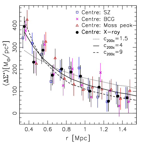
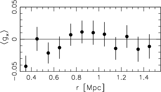
7.3 Stacked signal and constraints on the average cluster concentration
Miscentring reduces the shear signal at small radii. To test if our data show signs for this, we compare the stacked signal for the different centres (top panel of Fig. 17). To stack the signal from clusters at different redshifts and lensing efficiencies we employ the differential surface mass density (see Eq. 14), where we compute using the of the corresponding magnitude bin and colour selection scheme. Our clusters span a significant range in mass. Here we expect higher profiles for the more massive clusters. Before stacking, we therefore scale them to approximately the same signal amplitude. For this we compute a theoretical NFW model for the differential surface mass density for each cluster assuming its mass inferred from the SZ signal (Bleem et al., 2015)131313We weight according to the SZ mass and not the lensing-inferred mass. The latter is more noisy and would give higher weight to clusters for which the lensing mass estimate scatters up. and a fixed , and then scale the cluster signal as
| (31) |
We evaluate the theoretical model at an intermediate scale , but note that the exact choice is not important as we are only interested in an approximate rescaling to optimise the weighting. We then compute the weighted average
| (32) |
with and indicating the uncertainty of .
The results are shown in in the top panel of Fig. 17. We first note that the stacked profiles are fairly similar for the different centre definitions. This is also the case for an analysis centred on the peaks in the weak lensing mass reconstruction. Such an analysis should not suffer from miscentring, but is rather expected to deliver shear estimates that are biased high (see e.g. Dietrich et al., 2012). The similarity of the shear profiles suggests that, for the sample as a whole, miscentring appears to have relatively minor impact at the radial scales considered in our analysis.
We also fit the reduced shear profiles of all clusters using models with different fixed concentrations. For three of these fixed concentrations and the analysis using the X-ray centres we show the averaged best-fit models from all clusters in Fig. 17, using the same scale factors and weights as used for the data. In these fits we use an extended fit range 300 kpc to 1.5 Mpc to increase the sensitivity of the data for constraints on the concentration, which are mostly derived from the change in the slope between small and large radii (compare Fig. 17). Adding the from the individual clusters with equal weights we compute the total of the sample as function of the fixed concentration, allowing us to place constraints on the average concentration of the sample141414An alternative approach to constrain cluster concentrations from weak lensing data is to fit both mass and concentration simultaneously for each cluster. These individual constraints are however very weak due to shape noise, and they are strongly affected by large-scale structure projections (e.g. Hoekstra, 2003). to using the X-ray centres (), using the SZ centres (), using the BCG centres (), and () when centring on the weak lensing mass peaks. We stress that the fitting was conducted for each cluster separately (see Sect. 7.2), and that the stacked signal shown in Fig. 17 is for illustrative purposes only. This is important given that the scaling is only approximate, while the individual analyses account for all effects (e.g. reduced shear).
Due to miscentring the estimates using the X-ray, SZ, and BCG centres may be slightly biased low, while the estimate based on the mass peak centre is likely biased high. Given that all constraints are well consistent within the uncertainties, we conclude that miscentring has a negligible impact for the constraints on concentration at the current statistical precision. These estimates are consistent with predictions from recent numerical simulations. In particular, the relation from Diemer & Kravtsov (2015), which corresponds to our default analysis, yields average concentrations (average 3.8) in our mass and redshift range, fully consistent with our constraints. Accordingly, it is not surprising that it provides similarly good fits to the data as the best-fit fixed concentrations, e.g. we obtain with the Diemer & Kravtsov (2015) relation for the analysis using the X-ray centres. For comparison, the relation from Duffy et al. (2008) yields lower average concentrations (average 2.7) in our mass and redshift range, which agrees with our constraints at the level only.
In the bottom panel of Fig. 17 we additionally show the stacked profile of the reduced cross-shear component of all clusters measured with respect to their X-ray centres (computed without rescaling). We find that it is consistent with zero, providing another consistency check for our analysis.
7.4 Calibration of the mass estimates with simulations and consistency checks in the data
We have adopted a simplistic model for the mass distribution in clusters, namely a spherical NFW halo with a known centre and a concentration fixed by a concentration–mass relation. However, effects such as choosing an improper cluster centre (“miscentring”), variations in cluster density profiles, and noise bias in statistical estimators can introduce substantial biases in the mass constraints derived from fits of such a model to cluster weak lensing shear profiles (e.g. Becker & Kravtsov, 2011; Gruen et al., 2015). To estimate and correct for these biases in our analysis we apply our measurement procedure to a large sets of simulated cluster weak lensing data based on the Millennium XXL simulation (Angulo et al., 2012) and the simulations created by Becker & Kravtsov (2011, henceforth BK11). The details of this analysis will be presented in Applegate et al. (in prep.). Here we only summarise the most important points relevant to this analysis.
7.4.1 Simulations
The two simulations considered for our calibration differ in the redshifts of the available snapshots, in the cluster mass range, and the input cosmology. The difference in cosmology alters the concentration–mass relation in the simulation (e.g. Diemer & Kravtsov, 2015), but this is small compared to the range of relations we consider (Sect. 7.4.4). Likewise, the calibration does not depend on mass to a level that is important for this analysis when the full likelihood distribution of the mass constraints is used (see Applegate et al. in prep.). We find that the bias has some dependence on redshift and therefore interpolate between the two available snapshots that match our observations best. For the calibration of both and these are the snapshot of the BK11 simulation and the snapshot of the Millennium XXL simulation. Note that both simulations yield consistent bias calibrations at , where data are available from both simulations (see Applegate et al. in prep.).
For the BK11 snapshot we include 788 haloes with , providing a good match to the SPT cluster mass range. Since the sample provided to us by BK11 is selected in , we are only able to measure the bias in at , above which we are still complete. For the MXXL snapshot we include the 2100 most massive haloes, corresponding to . For the calibration of weak lensing estimates for this sample is complete for , matching the mass range of the studied SPT clusters well (compare to Table 1).
The generation of simulated shear fields from the underlying N-body simulations is described in BK11. In short, all particles within Mpc along the line-of-sight to each cluster are projected onto a common plane to produce a map, from which a fast Fourier transform can compute the shear field on a regular grid. The procedure is similar for MXXL, except that particles within Mpc are used, and three orthogonal projection directions are employed.
We create mock observations matching each cluster in our observed sample. We first select a profile centre location by randomly choosing an offset from the true cluster centre, which is defined as the position of the most-bound particle in the simulation, according to different probability distributions reflecting our assumptions on the miscentring distributions of SZ and X-ray centres (Sect. 7.4.2). We then bin and azimuthally average the simulated reduced shear grid, matching the binning in the observed shear profile, and add Gaussian random noise to each bin matching the observed noise levels. We fit the cluster masses from these simulated weak lensing data as done for the real clusters, calculating scans of versus . To obtain a bias calibration for the scaling relation analysis (see Sect. 8) we model the ratio , where denotes the corresponding halo mass, as a log-normal distribution. We associate the mean of the log-normal distribution as the inferred average bias and the width of the distribution as the intrinsic scatter from cluster triaxiality, substructure, and line-of-sight projections. We fit the log-normal distribution to the population of clusters in each snapshot, marginalising over the statistical uncertainty for each cluster (see Applegate et al. in prep). While we perform the analysis in bins of true halo mass to check for mass-dependence of the bias, we instead only use one all-encompassing mass bin to determine the bias for this analysis.
We repeat the whole procedure for a number of miscentring distributions and relations. We list individual bias numbers for each cluster for the X-ray and SZ miscentring distributions and the Diemer & Kravtsov (2015) relation in Table 6, and sample-averaged values for a number of configurations in Table 7. We stress that the quoted bias numbers are adequate for quantitative analyses that take the full likelihood distribution of the mass constraints into account, as done in our scaling relation analysis presented in Sect. 8. We correct the mass estimates as
| (33) |
As an approximation we also apply these bias correction factors to the maximum likelihood values and confidence intervals indicated in Figures 18 to 20 in the following sections. However, note that the bias factors may differ at some level for the maximum likelihood estimates and the fits that use the full likelihood distribution due to differences in the impact of noise bias. We plan to investigate this issue further in Applegate et al. (in prep.).
7.4.2 Miscentring distributions
For the SPT clusters we have proxies for the cluster centres, where we in particular use the X-ray centroids and SZ peaks for the mass analysis. These need to be related to the cluster centres defined by halo finding algorithms used to predict the cluster mass function from simulations. These offsets will typically lower the measured shear from the expected NFW signal at small radii (e.g. Johnston et al., 2007; George et al., 2012). To mimic this effect in the BK11 and MXXL N-body simulations, where we have neither mock SZ nor mock X-ray observations, we employ offset distributions derived from the Magneticum Pathfinder Simulation (Dolag, Komatsu & Sunyaev 2016; see also Bocquet et al. 2016), which is a large volume, high-resolution cosmological hydrodynamical simulation. It includes simulated SZ and X-ray observations, where we make use of SPT mock catalogues (Saro et al. 2014; Gupta et al. in prep.) that include the full SPT cluster detection procedure. We find that the most relevant parameter regarding the centring uncertainty when using the SZ centres is the smoothing scale used for the cluster detection (see Bleem et al., 2015). We therefore use the actual distribution of values for our clusters from Bleem et al. (2015) for the generation of the miscentring distribution.
| Miscentring | rel. | ||
|---|---|---|---|
| None | Diemer+15 | 0.95 | 0.96 |
| X-ray-hydro | Diemer+15 | 0.87 | 0.87 |
| SZ-hydro | Diemer+15 | 0.81 | 0.81 |
| SZ-hydro | 0.79 | 0.81 | |
| SZ-hydro | 0.89 | 0.86 | |
| SZ-hydro | 0.73 | 0.77 |
7.4.3 Impact and uncertainty of the miscentring correction
Using the default relation (Diemer & Kravtsov, 2015) and comparing the analyses using the miscentring distributions from the hydrodynamical simulation to the case without miscentring, we estimate that miscentring on average introduces a moderate mass bias of – when using the X-ray centres, and a more substantial bias of – using the SZ centres (see Table 7). The SZ measurements less accurately determine the cluster centre, which on-average increases the bias correction. This result is consistent with the smaller average offsets from the mass peaks found for the X-ray centres (Sect. 7.1).

As a consistency check for the miscentring correction we compare the bias-corrected mass estimates using the X-ray and SZ centres in Fig. 18. Their median ratio , with an uncertainty estimated by bootstrapping the clusters, is consistent with unity as expected in the case of accurate bias correction. We, however, note that the small sample size leads to a significant uncertainty of this median ratio, making it not a very stringent test for the accuracy of the bias correction.
The accurate correction for mass modelling biases such as the one introduced by miscentring is an active field of research (e.g. LSST Dark Energy Science Collaboration, 2012). Our analysis using a miscentring distribution based on a hydrodynamical simulation is a step forward in this respect, but we acknowledge that it is still simplistic. In particular, it ignores that positional offsets are not always in a random direction. This is prominently demonstrated by the merger SPT-CL 01024915, for which the location of the SZ peak is closer to the centre between the two peaks of the mass reconstruction (see Fig. 29), leading to an increased mass estimate (compare Fig. 18). Due to this simplification in our current analysis, we conservatively assign a large uncertainty for the miscentring correction, which amounts to 50% of the correction, corresponding to a 4% uncertainty in mass when using the X-ray centres and 7% when using the SZ centres. Future analyses can reduce this uncertainty by simulating all observables including the weak lensing data from the same hydrodynamical simulation (see Sect. 9.5).
7.4.4 Uncertainties in the concentration–mass relation
For the case of SZ miscentring Table 7 lists average bias numbers for the relation from Diemer & Kravtsov (2015), as well as fixed concentrations . Our bias correction procedure effectively maps the relation used for the fit to the observed relations in the simulations that are used for the bias correction (BK11, Millennium XXL). The remaining question is how well the relations in these simulations resemble the true average relation in the Universe, especially regarding the impact of baryons. Duffy et al. (2010) show that the impact of baryon physics appears to have only a relatively minor () influence on the concentrations of very massive clusters. De Boni et al. (2013) find similar numbers at low redshifts (for complete halo samples), and slightly stronger effects at (–%). Interpolating between the values in Table 7 we estimate that a 10–20% uncertainty on the concentration around leads to a – systematic uncertainty for the constraints on , where we conservatively adopt the larger number in our systematic error budget (see Sect. 7.5).
De Boni et al. (2013) note that differences in the definition of the concentration can lead to shifts in the values measured from N-body simulations of up to 20%. This is not a concern for our analysis, as we directly estimate the calibration from the simulated weak lensing data, and therefore do not rely on concentration measurements in the simulations.
| Current | Near future | |||||||
| Source | rel. error | rel. error | rel. error | rel. error | Sect./ | Improve via | ||
| signal | signal | App. | ||||||
| Shape measurements: | ||||||||
| Shear calibration | 4% | 6% | 1% | 1.5% | 5 | Image simulations | ||
| Redshift distribution: | ||||||||
| sys. photo- | 2.2% | 3.3% | 1.5% | 2.2% | 6.3.2 | Improved priors + | ||
| cosmic variance | 1% | 1.5% | 1% | 1.5% | 6.6 | More reference fields | ||
| deblending | 0.5% | 0.8% | 0% | 0% | B | F606W-detected photo-s | ||
| LCBG contamination | 0.9% | 1.4% | 0.5% | 0.8% | F | Apply model | ||
| Mass model: | ||||||||
| Miscentring for X-ray (SZ) centres | 4% (7%) | 2% (3.5%) | 7.4.2 | Hydro sims, weak lensing | ||||
| relation | 4% | 2% | 7.4.4 | Hydro sims, weak lensing | ||||
| Total for X-ray (SZ) centres : | 9.2% (10.8%) | 4.2% (5.1%) | ||||||
7.5 Statistical precision versus systematic uncertainty
We summarize the identified sources of systematic uncertainty for our study in Table 8, pointing to their corresponding sections, and listing their associated relative uncertainties in the measured weak lensing signal and mass constraints. Combining all systematic error contributions in quadrature, we estimate an overall systematic mass uncertainty of 9% (11%) for the analysis using the X-ray (SZ) centres. This can be compared to the combined statistical mass signal-to-noise ratio of the sample, which we approximate as
| (34) |
which corresponds to a precision, ignoring the impact of intrinsic scatter, e.g. from cluster triaxiality. Accordingly, our total uncertainty is dominated by statistical measurement noise and not systematic uncertainties.
For the analysis of larger future data sets with improved statistical precision it will be important to further reduce systematic uncertainties. When discussing the individual sources of systematic uncertainty we have already suggested strategies how their influence can be reduced in the future. The largest contributions to the systematic error budget currently come from the shear calibration, miscentring corrections, and uncertainties in the relation. All of these can be reduced with better simulations. For the latter two issues the weak lensing data can themselves provide information that help to reduce these uncertainties (see also Sect. 9.5). As a rough guess we expect that it should be possible to cut the systematic uncertainties associated with the mass modelling by half in the coming years with moderate effort (compare Table 8), and note that some improved shape measurement techniques have already reached significantly higher accuracy (e.g. Bernstein et al., 2016; Fenech Conti et al., 2017). We further discuss the strategies to reduce systematic uncertainties in Sect. 9.
8 Constraints on the – scaling relation
In the self-similar model (e.g. Kaiser & Silk, 1986) galaxy clusters form through the gravitational collapse of the most overdense regions in the early Universe. In this model the cluster baryons are heated through gravitational processes only, leading to predictions for cluster scaling relations. Deviations from self-similarity, e.g. regarding the slope of the X-ray luminosity–temperature relation (e.g. Arnaud & Evrard, 1999), suggest that non-gravitational effects, such as heating by active galactic nuclei or radiative cooling, provide non-negligible contributions to the energy budget of clusters. However, the redshift evolution of cluster X-ray observables appears to be consistent with self-similar predictions (e.g. Maughan et al., 2006), suggesting that non-gravitational effects have a similar impact at low and high redshifts. If this “weak self-similarity” (e.g. Bower, 1997) also applies to cluster masses, we expect a scaling between temperature and mass in the form
| (35) |
(e.g. Mathiesen & Evrard, 2001; Böhringer, Dolag & Chon, 2012), where
| (36) |
indicates the redshift dependence of the Hubble parameter, here assuming a flat CDM cosmology, and corresponds to the self-similar prediction for the slope of the relation.
The main constraints on cluster scaling relations from our sample will be presented in a forthcoming paper (Dietrich et al. in prep.) that combines our measurements with a complementary sample of clusters at lower redshifts with Magellan/Megacam observations and accounts for the SPT selection function, which is especially important when calibrating SZ scaling relations. However, here we already combine our measurements with core-excised Chandra X-ray temperature estimates that are available for 12 clusters in our sample. Details of the specific measurements are provided in McDonald et al. (2013), with the analysis pipeline adapted based on Vikhlinin et al. (2006). In short, Chandra ACIS-I data were reduced using ciao v4.7 and caldb v4.7.1. All exposures were initially filtered for flares, before applying the latest calibrations and determining the appropriate epoch-based blank-sky background. Point sources were identified via an automated wavelet decomposition technique (Vikhlinin et al., 1998) and masked. Spectra were extracted in a core-excised region from – (McDonald et al., 2013) and fit over 0.5–10.0 keV using a combination of an absorbed, optically-thin plasma (phabsapec), an absorbed hard background component (phabsbremss), and a soft background (apec), see McDonald et al. (2013) for details.
Figures 19 and 20 show the bias-corrected using the Diemer & Kravtsov (2015) relation as function of the core-excised estimates (Table 9) for the analyses centring on the X-ray centroids or SZ peaks, respectively. For comparison we show best-fit estimates for the scaling relation derived by Arnaud, Pointecouteau & Pratt (2005, based on their keV sample), Vikhlinin et al. (2009a), and Mantz et al. (2016) using clusters at lower and intermediate redshifts ().
To obtain quantitative constraints on the scaling relation, we assume the functional form
| (37) |
where the temperature pivot point roughly corresponds to the mean temperature of the sample. Our fitting method is based on the approach of Kelly (2007), which incorporates measurement errors in the - and - coordinates and has been extended to include log-normal intrinsic scatter. The method has been generalized to use the exact likelihood from the lensing analysis, and a two-piece normal approximation to the X-ray likelihood (Applegate et al., 2016). For this analysis we use the lensing likelihood based on the dominant shape noise only and absorb the minor contributions from large-scale structure projections and line-of-sight variations in the redshift distribution (see Sect. 7.2) in the intrinsic scatter .
| Cluster | [keV] |
|---|---|
| SPT-CL 00005748 | |
| SPT-CL 01024915 | |
| SPT-CL 05335005 | |
| SPT-CL 05465345 | |
| SPT-CL 05595249 | |
| SPT-CL 06155746 | |
| SPT-CL 21065844 | |
| SPT-CL 23315051 | |
| SPT-CL 23375942 | |
| SPT-CL 23415119 | |
| SPT-CL 23425411 | |
| SPT-CL 23595009 |
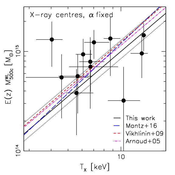
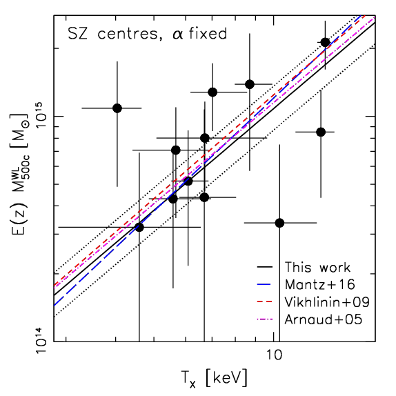
We fix the slope of the scaling relation to the self-similar prediction () for the current analysis, given the limited sample size and mass range. We then obtain constraints for our default analysis using the X-ray centres. When alternatively using the SZ peaks as centre for the weak lensing analysis we obtain consistent results . In addition to these statistical uncertainties there is a 9% (11%) systematic uncertainty for the analysis using the X-ray (SZ) centres, directly propagating into the normalisation of the scaling relation (see Sect. 7.5). The obtained constraints are consistent with the aforementioned results from lower redshift samples when assuming self-similar redshift evolution within (see Figures 19 and 20).
Jee et al. (2011) present an HST weak lensing analysis for 27 galaxy clusters at
, using a heterogeous sample that includes optically, NIR, and X-ray-selected clusters.
Their analysis suggests
a possible evolution in the – scaling relation
in comparison to self-similar extrapolations from lower redshifts.
For example, at keV their estimated scaling relation
has a lower amplitude by (statistical uncertainty from
Jee et al. (2011) only)
compared to the best-fit relation from
Arnaud, Pointecouteau & Pratt (2005).
We do not find significant indications for a similar evolution for the
– scaling relation,
but note that our statistical uncertainties are significantly larger given
our smaller sample size and more conservative radial fit range.
There are various additional differences in the analyses, such as different samples for the calibration of the
source redshift distribution, our more conservative removal of cluster
galaxies, and our calibration of modelling biases on simulations, making the
direct comparison difficult.
Importantly, both studies use different overdensities for the scaling
relation constraints151515We do not report masses as these are not
available in the BK11 simulation, preventing us to compute
accurate bias corrections for this overdensity..
Furthermore, Jee et al. (2011) use X-ray temperature estimates from the
literature that typically do not exclude the core regions.
Including the cores should, on average, reduce the temperatures in the presence
of cool-core clusters.
This would, however, aggravate the tension between the Jee et al. (2011) results
and the self-similar extrapolations from lower redshift samples.
9 Discussion
In our analysis we have introduced a number of new aspects and systematic investigations for weak lensing studies of high-redshift clusters. Here we discuss their relevance also in the context of future weak lensing programmes. Our study using HST and VLT data provides a demonstration for future weak lensing science investigations that combine deep high-resolution space-based shape measurements, e.g. from Euclid (Laureijs et al., 2011) or WFIRST (Spergel et al., 2015), with deep photometry, e.g. from LSST (LSST Science Collaboration et al., 2009).
9.1 The benefits and challenges of using faint blue galaxies for weak lensing
For deep weak lensing surveys conducting shape measurements at optical wavelengths the majority of the high-redshift (–) sources are blue star forming galaxies observed at rest-frame UV wavelengths with blue observed optical colours (see the top left panel of Fig. 5). These galaxies are useful as the source sample in weak lensing studies of high-redshift clusters both because of their high source density and high geometric lensing efficiency, but also because they can be readily distinguished from both blue and red cluster galaxies using optical colours (see Sect. 6.2). This enables a nearly complete removal of cluster galaxies from the weak lensing source sample, which is important both in order to minimise modelling uncertainties regarding cluster member contamination (Appendix E), and to ensure that intrinsic alignments of galaxies within the targeted clusters cannot bias mass constraints (but note that this appears to be a negligible effect at the precision of current samples, see Sifón et al., 2015).
To exploit these benefits, a number of challenges need to be overcome. Here we first stress that high signal-to-noise optical photometry is needed to robustly select these galaxies in colour space. In the case of our study a well-matched colour selection was possible in areas covered by ACS in both F606W and F814W. However, outside the F814W footprint we had to rely on the combination of F606W ACS imaging and VLT images, which, despite a good VLT integration time ks and seeing, delivered a density of usable sources that is only 32% of the density from the ACS-only selection (Sect. 6.8.1). This highlights that future weak lensing programmes and surveys should carefully tune the relative depth of their bands (regarding both red and blue filters) to maximise the science output of their data.
While our analysis is based on simple colour cuts due to the limited data available in our cluster fields, we expect that similar conclusions apply for surveys that aim at computing individual photometric redshifts for the weak lensing source galaxies. Photometric redshift selections correspond to higher dimensional cuts in colour-colour space. However, depending on the survey characteristics, the large population of blue high- galaxies may only be detected in a few of the bluer optical pass bands, effectively reducing photo- cuts to a selection in a relatively small colour-colour space. As a result, individual photometric redshift estimates for faint blue galaxies have typically large uncertainties unless deep photometry is available over a very broad wavelength range (in particular including deep -band and NIR observations). For cluster weak lensing studies noise in individual photometric redshifts is not a problem as long as cluster galaxies can be removed robustly and the overall source redshift distribution can be modelled accurately.
9.2 Robust estimates of the source redshift distribution
We employ a statistically consistent selection of source galaxies matched in filter, magnitude, colour, and shape properties in our cluster fields and observations of the CANDELS fields. This allows us to estimate the average source redshift distribution and its statistical variation between lines-of-sights using the CANDELS data and apply this information for the cluster weak lensing analyses. At depths similar to our data, the CANDELS fields are currently among the extragalactic fields that are best studied both photometrically and spectroscopically. We have shown that they cover enough sky area to reduce the cosmic variance contribution to the uncertainty on the mean lensing efficiency at our cluster redshifts to the level (Sect. 6.6), which is much smaller than current statistical weak lensing uncertainties. Therefore, we expect that the CANDELS fields will remain to be an important calibration sample for estimates of the source redshift distribution in deep weak lensing data in the near future.
As revealed by our comparison to HUDF data (Sect. 6.3.1) and confirmed via spatial cross-correlations with spectroscopic/grism redshifts (Appendix C), the 3D-HST CANDELS photo-s suffer from catastrophic redshift outliers (primarily galaxies at that are assigned a low photometric redshift ) and redshift focussing effects at . Together these would on average bias our mass estimates high by 12% if not accounted for. For our current study we have implemented an empirical correction for these systematics effects. We plan to investigate this issue and its causes in detail in a future paper (Raihan et al. in prep.). Given the high photometric quality, depth, and broad wavelength coverage of the CANDELS data, we speculate that some other current photometric redshift data sets might suffer from similar effects. This is supported by the weak lensing analyses of S10 and Heymans et al. (2012) as discussed in Sect. 6.3. We therefore expect that also other weak lensing programmes will have to implement similar correction schemes or improved photometric redshift algorithms, and apply these either to deep field data in case of colour cut analyses, or their survey data in case of individual photo- estimates. Surveys that obtain individual photo-s can also attempt to identify and remove galaxies in problematic ranges at the cost of reduced sensitivity. We stress that the use of the average redshift posterior probability distribution instead of the peak photometric redshift estimates is not sufficient to cure the identified issue for the 3D-HST photo-s (Sect. 6.3.4).
One route to calibrate photo-s is via very deep spectroscopy for representative galaxy samples. At present, such spectroscopic samples are very incomplete at the depth of our analysis, which is why we resorted to the comparison of the CANDELS photo-s to photometric redshifts for the HUDF (Rafelski et al., 2015), which are based on deeper data and a broader wavelength coverage. We find that this is a viable approach at the precision of current and near-term high- cluster samples with weak lensing measurements, but it is likely not of sufficient accuracy for the calibration of very large future data sets. To prepare for the analyses of such data sets it is vital and timely to obtain larger spectroscopic calibration samples, including both highly complete deep samples for direct calibration, but also very large, potentially shallower and less complete samples Newman et al. (2015). The later can be used to infer information on the redshift distribution via spatial cross-correlations (e.g. Newman, 2008; Matthews & Newman, 2010; Schmidt et al., 2013; Rahman et al., 2015, 2016), for which we provide one of the first practical applications in the context of weak lensing measurements (see Appendix C and Hildebrandt et al., 2017).
As an important ingredient for our modelling of the redshift distribution we carefully matched the selection criteria and noise properties between our cluster field data and the CANDELS data to ensure that consistent galaxy populations are selected between both data sets (see Sect. 6.4 and Appendix D.3). For the colours obtained from the combination of ACS F606W and VLT data we empirically estimated the net scatter distribution by comparing to the colours estimated in the inner cluster regions from ACS F606W and F814W data. We note that systematic effects such as residuals from the PSF homogenisation can add scatter which may well deviate from Poisson noise distributions that are often assumed, e.g. in photometric redshift codes. As we empirically sample from the actual scatter distribution such effects are automatically accounted for in our analysis. For future surveys that vary in data quality we recommend to obtain repeated imaging observations of spectroscopic reference fields that span the full range of varying observing conditions, in order to generate similar empirical models for the impact of the actual noise properties.
9.3 Accounting for magnification
The impact of weak lensing magnification on the source redshift distribution has typically been ignored in past weak lensing studies. Our investigation of this effect in Sect. 6.7 indicates that the net effect is small for our study given the depth of our data. However, shallower programmes such as DES (The Dark Energy Survey Collaboration, 2005) or KiDS (Kuijken et al., 2015), which aim to calibrate high- cluster masses by combining measurements from a large number of clusters, will need to carefully account for the resulting boost in the average lensing efficiency . For example, Fig. 11 illustrates that the impact of magnification on the source redshift distribution has a larger impact on the reduced shear profile at brighter magnitudes than the typically applied correction for the finite width of the source redshift distribution.
We point out that knowledge of the redshift distribution is needed at fainter magnitudes than the targeted depth limit of a survey in order to be able to compute the actual correction for the impact of magnification (Sect. 6.7). Accordingly, it is necessary to obtain spectroscopic redshift samples for photo- calibration to greater depth than the targeted survey depth. The difference in depth depends on the maximum magnification that is considered, and therefore the magnitude limit, the cluster redshift and mass, as well as the considered fit range.
We also note that it is important to take magnification into account when using the source density and the density profiles as validation tests for the cluster member removal (see Sect. 6.8). Programmes with ground-based resolution will also need to account for the change in source sizes due to magnification as function of redshift, cluster-centric distance, and mass, as shape cuts could otherwise introduce redshift- and mass-dependent selection biases.
9.4 Shape measurement biases
Currently the shear calibration uncertainty constitutes the largest individual contribution to the systematic error budget of our study (4% for the shear calibration corresponding to a 6% mass uncertainty). This is due to the fact that we base the calibration on simulations from the STEP project (Sect. 5.1) which lack faint galaxies that influence the bias calibration (Hoekstra et al., 2015) and do not probe shears as high as those used in our analysis. However, this source of systematics can easily be reduced through image simulations that resemble real galaxy populations and cluster-regime shears more accurately, and which can be generated recent tools such as GalSim (Rowe et al., 2015). We therefore expect that shear measurement biases in cluster weak lensing studies will soon be reduced to the levels reached in cosmic shear measurements (e.g. Fenech Conti et al., 2017). Also see Hoekstra, Viola & Herbonnet (2017), whose results suggest that the impact of the higher density of sources in cluster regions on shape measurement biases should be negligible for current data.
In addition, additive shape measurement biases can be relevant for cluster weak lensing in particular for pointed follow-up programmes where the clusters are always centred at similar detector positions. An example for such a potential source of bias can be CTI residuals. However, through a new null test we have shown that our data show no significant CTI-like residuals within the current statistical uncertainty (Sect. 5.2).
9.5 Accounting for biases in the mass modelling
We have calibrated our mass estimates using reduced shear profile fits to simulated cluster weak lensing data from N-body simulations (see Sect. 7.4). One important source for bias is miscentring of the reduced shear profile. As we do not know the location of the centre of the 3D cluster potential we have to rely on observable proxies for the cluster centre, leading to a suppression of the expected reduced shear signal at small radii. Based on the work from Dietrich et al. (2012) we expect that the peaks in the reconstructed weak lensing mass maps of the clusters (see Sect. 7.1) should provide a tight tracer for the centre of the 3D cluster potential, but we do not use these centres for our mass constraints in our current analysis as they are expected to yield masses that are biased high. By studying the offset distributions between the mass peaks and the other proxies for the cluster centre we find that the X-ray centroids provide the smallest average offsets, closely followed by the SZ peak locations. Hence, they also provide good proxies for the cluster centre, which is why we employ them as centres for our mass constraints. To account for the expected remaining bias caused by miscentring, we randomly misplace the centre in the simulated weak lensing data based on offset distributions measured between the 3D cluster centre and the SZ peak location or X-ray centroid in hydrodynamical simulations (see Sect. 7.4.2). Future studies could further advance this approach by simulating all observables including SZ, X-ray, and weak lensing data from the same hydrodynamical simulation, in order to also account for possible covariances between these observables. Our analysis of the prominent merger SPT-CL 01024915 demonstrates that such covariances exist, as both the X-ray centroid and SZ peak are located between the two peaks of the mass reconstruction (see Fig. 29). Hence, the misplacement is not in a random direction. To validate the accuracy of the employed simulations, the measured offset distributions between the mass peaks and the different proxies for the centre can be compared between the real data and the simulations. This approach could be further expanded by explicitly accounting for the miscentring in the fitted reduced shear profile model (e.g. Johnston et al. 2007; George et al. 2012; also see Köhlinger, Hoekstra & Eriksen 2015 for the impact of miscentring in stacked Stage IV analyses).
A further uncertainty for the mass constraints arises from uncertainties in the assumed relation. The applied calibration procedure essentially maps the measurements onto the relation of the simulation. Remaining uncertainties reflect our ability to simulate the true relation of the Universe, especially with respect to the impact of baryons. These uncertainties are expected to shrink with further advances in simulations, in particular thanks to the recent advent of large hydrodynamical simulations (e.g. Dolag, Komatsu & Sunyaev, 2016). In addition, the weak lensing measurements themselves can be used to test if the inferred reduced shear profiles are consistent with the simulation-based priors on the relation, in particular if information from the inner reduced shear profiles is incorporated. Using the X-ray centroids our analysis yields a best-fitting fixed concentration for the sample of when including scales kpc (Sect. 7.3). This is fully consistent with recent results for the relation from simulations (e.g. Diemer & Kravtsov, 2015), but higher than earlier results from Duffy et al. (2008), which, however, are based on a WMAP5 cosmology (Komatsu et al., 2009) with lower and , reducing the resulting concentrations. We note that future studies that aim to obtain tighter constraints on the concentration will have to account for the impact of miscentring and stronger shears in the inner cluster regions, which we could ignore for this part of our analysis given the statistical uncertainties.
10 Conclusions
We have presented a weak gravitational lensing analysis of 13 high-redshift clusters from the SPT-SZ Survey, based on shape measurements in high resolution HST/ACS data and colour measurements that also incorporate VLT/FORS2 imaging. We have introduced new methods for the weak lensing analysis of high redshift clusters and carefully investigated the impact of systematic uncertainties as discussed in Sect. 9 in the context of future programmes. In particular, we select blue galaxies in colour to achieve a nearly complete removal of cluster galaxies, while selecting most of the relevant source galaxies at (see Sect. 6.2). Carefully matching our selection criteria we estimate the source redshift distribution using data from CANDELS, where we apply a statistical correction for photometric redshift outliers. This correction is derived from the comparison to deep spectroscopic and photometric data from the HUDF (see Sect. 6.3), and checked using spatial cross-correlations (see Appendix C). We account for the impact of lensing magnification on the source redshift distribution, which we find is especially important for shallower surveys (see Sect. 6.7). We also introduce a new test for residual contamination of galaxy shape estimates from charge-transfer inefficiency, which is in particular applicable for pointed cluster follow-up observations (see Sect. 5.2). Finally, we account for biases in the mass modelling through simulations (see Sect. 7.4).
At present, our weak lensing mass constraints are limited by statistical uncertainties given the small cluster sample and the limited depth of the data for the colour selection in the cluster outskirts. For the current study the total systematic uncertainty on the cluster mass scale at high- is at the level, where the largest contributions come from the shear calibration and mass modelling. As discussed in Sect. 7.5 we have identified strategies how this can be reduced to the level in the near future based on exisiting calibration data and improved simulations. This is particularly relevant for near-term studies using larger HST data sets.
We have used our measurements to derive updated constraints on the – scaling relation for massive high- clusters in combination with Chandra observations. Compared to scaling relations calibrated at lower redshifts we find no indication for a significant deviation from self-similar redshift evolution at our current precision (see Sect. 8). Our measurements will additionally be used in companion papers to derive updated constraints on additional mass-observable scaling relations, where we also incorporate weak lensing measurements at lower redshifts from Magellan/Megacam (Dietrich et al. in prep.) and the Dark Energy Survey (DES, The Dark Energy Survey Collaboration, 2005, Stern et al. in prep.), and to derive improved cosmological constraints from the SPT-SZ cluster sample.
We investigate the offset distributions between different proxies for the cluster centre and the weak lensing mass reconstruction, where we find that the X-ray centres provide the smallest average offsets (see Sect. 7.1). Our analysis constrains the average concentration of the cluster sample to (Sect. 7.3) when using the X-ray centres and including information from smaller scales (), which are excluded for the conservative mass constraints.
With the advent of the next generation of deep cluster surveys such as SPT-3G (Benson et al., 2014), the Dark Energy Survey (DES The Dark Energy Survey Collaboration, 2005), Hyper-Suprimecam (HSC Miyazaki et al., 2012), eROSITA (Merloni et al., 2012), and Advanced ACTPol (Henderson et al., 2016) it will be vital to further tighten the weak lensing calibration of cluster masses in order to exploit these surveys for constraints on cosmology and cluster astrophysics. At low and intermediate redshifts, weak lensing surveys such as DES, HSC, and KiDS are expected to soon calibrate cluster masses at the few per cent level, especially if large numbers of clusters can be reliably selected down to lower masses and if their weak lensing signatures are combined statistically (e.g. Rozo, Wu & Schmidt, 2011). Such surveys will also provide some statistical weak lensing constraints for clusters out to (e.g. van Uitert et al., 2016), but it still needs to be demonstrated how reliably such measurements can be conducted from the ground as most of the distant background galaxies are poorly resolved. At such cluster redshifts HST is currently unique with its capabilities to measure robust individual cluster masses with good signal-to-noise. Clusters at high redshifts and high masses are very rare. As a result, stacking analyses of shallower wide-area surveys cannot compete in terms of precision for their mass calibration with a large HST program that obtains pointed follow-up observations for all of them. Our current study is an important pathfinder towards such a program. For comparison, stacked analyses tend to be more powerful for lower mass clusters, which are too numerous to be followed up individually. The combination of deep pointed follow-up for high-mass clusters and stacked shallower measurements for lower mass clusters is therefore particularly powerful for obtaining constraints on the slope of mass-observable scaling relations. In addition, good signal-to-noise ratios for individual clusters, as provided by deep pointed follow-up, are needed for constraints on intrinsic scatter.
In the 2020s weak lensing Stage IV dark energy experiments such as Euclid (Laureijs et al., 2011), LSST (LSST Science Collaboration et al., 2009), and WFIRST (Spergel et al., 2015) are expected to provide a precise calibration of cluster masses over a wide range in redshift (for a forecast for Euclid see Köhlinger, Hoekstra & Eriksen, 2015). To reach their weak lensing science goals they will require highly accurate calibrations for the redshift distribution and shear estimation. Further efforts will be needed to fully exploit these calibrations and weak lensing data sets for cluster mass estimation. For example, the shear calibration needs to be extended towards stronger shear, and magnification has to be taken into account when estimating the source redshift distribution (Sect. 9.3). We also stress that it will be vital to pair such observational studies with analyses of large sets of hydrodynamical simulations, in order to accurately calibrate the weak lensing mass estimates and account for covariances with other observables (see Sect. 9.5).
LSST and Euclid will still have signficantly lower densities of high-redshift background source galaxies compared to HST observations. In order to extend the mass calibration for massive clusters out to very high redshifts (), large pointed HST and subsequently JWST programmes may therefore remain the most effective approach until similarly deep data become available from WFIRST.
Acknowledgements
This work is based on observations made with the NASA/ESA Hubble Space Telescope, using imaging data from the SPT follow-up GO programmes 12246 (PI: C. Stubbs) and 12477 (PI: F. W. High), as well as archival data from GO programmes 9425, 9500, 9583, 10134, 12064, 12440, and 12757, obtained via the data archive at the Space Telescope Science Institute, and catalogues based on observations taken by the 3D-HST Treasury Program (GO 12177 and 12328) and the UVUDF Project (GO 12534, also based on data from GO programmes 9978, 10086, 11563, 12498). STScI is operated by the Association of Universities for Research in Astronomy, Inc. under NASA contract NAS 5-26555. It is also based on observations made with ESO Telescopes at the La Silla Paranal Observatory under programmes 086.A-0741, 088.A-0796, 088.A-0889, 089.A-0824. The scientific results reported in this article are based in part on observations made by the Chandra X-ray Observatory (ObsIDs 9332, 9333, 9334, 9335, 9336, 9345, 10851, 10864, 11738, 11739, 11741, 11742, 11748, 11799, 11859, 11864, 11870, 11997, 12001, 12002, 12014, 12091, 12180, 12189, 12258, 12264, 13116, 13117, 14017, 14018, 14022, 14023, 14349, 14350, 14351, 14437, 15572, 15574, 15579, 15582, 15588, 15589, 18241).
It is a pleasure to thank Gabriel Brammer, Pieter van Dokkum, Mattia Fumagalli, Ivelina Momcheva, Rosalind Skelton, and the 3D-HST team for helpful discussions and for making their photometric and grism redshift catalogues available to us prior to public release. We thank Matthew Becker and Andrey Kravtsov for making results from their N-body simulation (Becker & Kravtsov, 2011) available to us, Raul Angulo for providing data from the Millennium XXL Simulation, and Klaus Dolag for providing access to data from the Magneticum Pathfinder Simulation.
TS, DA, and FR acknowledge support from the German Federal Ministry of Economics and Technology (BMWi) provided through DLR under projects 50 OR 1210, 50 OR 1308, 50 OR 1407, and 50 OR 1610. TS also acknowledges support from NSF through grant AST-0444059-001 and SAO through grant GO0-11147A. This work was supported in part by the Kavli Institute for Cosmological Physics at the University of Chicago through grant NSF PHY-1125897 and an endowment from the Kavli Foundation and its founder Fred Kavli. HH acknowledges support from NWO VIDI grant number 639.042.814 and ERC FP7 grant 279396. Work at Argonne National Laboratory was supported under U.S. Department of Energy contract DE-AC02-06CH11357. The Munich group acknowledges the support by the DFG Cluster of Excellence “Origin and Structure of the Universe” and the Transregio program TR33 “The Dark Universe”. R.J.F. is supported in part by fellowships from the Alfred P. Sloan Foundation and the David and Lucile Packard Foundation. TdH is supported by a Miller Research Fellowship. PS acknowledges support by the European DUEL Research-Training Network (MRTN-CT-2006-036133) and by the Deutsche Forschungsgemeinschaft under the project SCHN 342/7-1. CBM acknowledges the support of the DFG under Emmy Noether grant Hi 1495/2-1. BB is supported by the Fermi Research Alliance, LLC under Contract No. De-AC02-07CH11359 with the United States Department of Energy. CR acknowledges support from the Australian Research Council’s Discovery Projects scheme (DP150103208). The Dark Cosmology Centre is funded by the Danish National Research Foundation.
References
- Albrecht et al. (2006) Albrecht A. et al., 2006, astro-ph/0609591
- Allen, Evrard & Mantz (2011) Allen S. W., Evrard A. E., Mantz A. B., 2011, ARA&A, 49, 409
- Andersson et al. (2011) Andersson K. et al., 2011, ApJ, 738, 48
- Angulo et al. (2012) Angulo R. E., Springel V., White S. D. M., Jenkins A., Baugh C. M., Frenk C. S., 2012, MNRAS, 426, 2046
- Applegate et al. (2016) Applegate D. E. et al., 2016, MNRAS, 457, 1522
- Applegate et al. (2014) Applegate D. E. et al., 2014, MNRAS, 439, 48
- Arnaud & Evrard (1999) Arnaud M., Evrard A. E., 1999, MNRAS, 305, 631
- Arnaud, Pointecouteau & Pratt (2005) Arnaud M., Pointecouteau E., Pratt G. W., 2005, A&A, 441, 893
- Bartelmann & Schneider (2001) Bartelmann M., Schneider P., 2001, Phys. Rep., 340, 291
- Battaglia et al. (2016) Battaglia N. et al., 2016, JCAP, 8, 013
- Bayliss et al. (2016) Bayliss M. B. et al., 2016, ApJS, 227, 3
- Becker & Kravtsov (2011) Becker M. R., Kravtsov A. V., 2011, ApJ, 740, 25
- Beckwith et al. (2006) Beckwith S. V. W. et al., 2006, AJ, 132, 1729
- Benítez (2000) Benítez N., 2000, ApJ, 536, 571
- Benítez et al. (2004) Benítez N. et al., 2004, ApJS, 150, 1
- Benjamin et al. (2013) Benjamin J. et al., 2013, MNRAS, 431, 1547
- Benson et al. (2014) Benson B. A. et al., 2014, in Society of Photo-Optical Instrumentation Engineers (SPIE) Conference Series, Vol. 9153, Society of Photo-Optical Instrumentation Engineers Conference Series, p. 1
- Benson et al. (2013) Benson B. A. et al., 2013, ApJ, 763, 147
- Bernstein et al. (2016) Bernstein G. M., Armstrong R., Krawiec C., March M. C., 2016, MNRAS, 459, 4467
- Bertin & Arnouts (1996) Bertin E., Arnouts S., 1996, A&AS, 117, 393
- Bleem et al. (2015) Bleem L. E. et al., 2015, ApJS, 216, 27
- Bocquet et al. (2016) Bocquet S., Saro A., Dolag K., Mohr J. J., 2016, MNRAS, 456, 2361
- Bocquet et al. (2015) Bocquet S. et al., 2015, ApJ, 799, 214
- Böhringer, Dolag & Chon (2012) Böhringer H., Dolag K., Chon G., 2012, A&A, 539, A120
- Bonnett (2015) Bonnett C., 2015, MNRAS, 449, 1043
- Bower (1997) Bower R., 1997, MNRAS, 288, 355
- Brammer, van Dokkum & Coppi (2008) Brammer G. B., van Dokkum P. G., Coppi P., 2008, ApJ, 686, 1503
- Brammer et al. (2012) Brammer G. B. et al., 2012, ApJS, 200, 13
- Brammer et al. (2013) Brammer G. B., van Dokkum P. G., Illingworth G. D., Bouwens R. J., Labbé I., Franx M., Momcheva I., Oesch P. A., 2013, ApJ, 765, L2
- Broadhurst, Taylor & Peacock (1995) Broadhurst T. J., Taylor A. N., Peacock J. A., 1995, ApJ, 438, 49
- Brodwin et al. (2010) Brodwin M. et al., 2010, ApJ, 721, 90
- Bruzual & Charlot (2003) Bruzual G., Charlot S., 2003, MNRAS, 344, 1000
- Carlstrom et al. (2011) Carlstrom J. E. et al., 2011, PASP, 123, 568
- Chiu et al. (2016a) Chiu I. et al., 2016a, MNRAS, 457, 3050
- Chiu et al. (2016b) Chiu I. et al., 2016b, MNRAS, 455, 258
- Coe et al. (2006) Coe D., Benítez N., Sánchez S. F., Jee M., Bouwens R., Ford H., 2006, AJ, 132, 926
- Crawford et al. (2006) Crawford S. M., Bershady M. A., Glenn A. D., Hoessel J. G., 2006, ApJ, 636, L13
- Crawford, Wirth & Bershady (2014) Crawford S. M., Wirth G. D., Bershady M. A., 2014, ApJ, 786, 30
- Crawford et al. (2011) Crawford S. M., Wirth G. D., Bershady M. A., Hon K., 2011, ApJ, 741, 98
- Crawford et al. (2016) Crawford S. M., Wirth G. D., Bershady M. A., Randriamampandry S. M., 2016, ApJ, 817, 87
- Davis et al. (2007) Davis M. et al., 2007, ApJ, 660, L1
- De Boni et al. (2013) De Boni C., Ettori S., Dolag K., Moscardini L., 2013, MNRAS, 428, 2921
- de Haan et al. (2016) de Haan T. et al., 2016, ApJ, 832, 95
- Diemer & Kravtsov (2015) Diemer B., Kravtsov A. V., 2015, ApJ, 799, 108
- Dietrich et al. (2012) Dietrich J. P., Böhnert A., Lombardi M., Hilbert S., Hartlap J., 2012, MNRAS, 419, 3547
- Dolag, Komatsu & Sunyaev (2016) Dolag K., Komatsu E., Sunyaev R., 2016, MNRAS
- Duffy et al. (2008) Duffy A. R., Schaye J., Kay S. T., Dalla Vecchia C., 2008, MNRAS, 390, L64
- Duffy et al. (2010) Duffy A. R., Schaye J., Kay S. T., Dalla Vecchia C., Battye R. A., Booth C. M., 2010, MNRAS, 405, 2161
- Erben et al. (2005) Erben T. et al., 2005, Astronomische Nachrichten, 326, 432
- Erben et al. (2001) Erben T., Van Waerbeke L., Bertin E., Mellier Y., Schneider P., 2001, A&A, 366, 717
- Fenech Conti et al. (2017) Fenech Conti I., Herbonnet R., Hoekstra H., Merten J., Miller L., Viola M., 2017, MNRAS, 467, 1627
- Foley et al. (2011) Foley R. J. et al., 2011, ApJ, 731, 86
- Ford et al. (2015) Ford J. et al., 2015, MNRAS, 447, 1304
- George et al. (2012) George M. R. et al., 2012, ApJ, 757, 2
- Giavalisco et al. (2004) Giavalisco M. et al., 2004, ApJ, 600, L93
- Grogin et al. (2011) Grogin N. A. et al., 2011, ApJS, 197, 35
- Gruen et al. (2015) Gruen D., Seitz S., Becker M. R., Friedrich O., Mana A., 2015, MNRAS, 449, 4264
- Gruen et al. (2014) Gruen D. et al., 2014, MNRAS, 442, 1507
- Haiman, Mohr & Holder (2001) Haiman Z., Mohr J. J., Holder G. P., 2001, ApJ, 553, 545
- Hartlap et al. (2009) Hartlap J., Schrabback T., Simon P., Schneider P., 2009, A&A, 504, 689
- Hasselfield et al. (2013) Hasselfield M. et al., 2013, JCAP, 7, 8
- Henderson et al. (2016) Henderson S. W. et al., 2016, Journal of Low Temperature Physics
- Heymans et al. (2006) Heymans C. et al., 2006, MNRAS, 368, 1323
- Heymans et al. (2012) Heymans C. et al., 2012, MNRAS, 427, 146
- High et al. (2012) High F. W. et al., 2012, ApJ, 758, 68
- Hilbert et al. (2009) Hilbert S., Hartlap J., White S. D. M., Schneider P., 2009, A&A, 499, 31
- Hildebrandt et al. (2017) Hildebrandt H. et al., 2017, MNRAS, 465, 1454
- Hinshaw et al. (2013) Hinshaw G. et al., 2013, ApJS, 208, 19
- Hoekstra (2001) Hoekstra H., 2001, A&A, 370, 743
- Hoekstra (2003) Hoekstra H., 2003, MNRAS, 339, 1155
- Hoekstra (2007) Hoekstra H., 2007, MNRAS, 379, 317
- Hoekstra et al. (2013) Hoekstra H., Bartelmann M., Dahle H., Israel H., Limousin M., Meneghetti M., 2013, Space Science Rev., 177, 75
- Hoekstra et al. (2011a) Hoekstra H., Donahue M., Conselice C. J., McNamara B. R., Voit G. M., 2011a, ApJ, 726, 48
- Hoekstra, Franx & Kuijken (2000) Hoekstra H., Franx M., Kuijken K., 2000, ApJ, 532, 88
- Hoekstra et al. (1998) Hoekstra H., Franx M., Kuijken K., Squires G., 1998, ApJ, 504, 636
- Hoekstra et al. (2011b) Hoekstra H., Hartlap J., Hilbert S., van Uitert E., 2011b, MNRAS, 412, 2095
- Hoekstra et al. (2015) Hoekstra H., Herbonnet R., Muzzin A., Babul A., Mahdavi A., Viola M., Cacciato M., 2015, MNRAS, 449, 685
- Hoekstra et al. (2012) Hoekstra H., Mahdavi A., Babul A., Bildfell C., 2012, MNRAS, 427, 1298
- Hoekstra, Viola & Herbonnet (2017) Hoekstra H., Viola M., Herbonnet R., 2017, MNRAS, 468, 3295
- Ilbert et al. (2009) Ilbert O. et al., 2009, ApJ, 690, 1236
- Israel et al. (2012) Israel H., Erben T., Reiprich T. H., Vikhlinin A., Sarazin C. L., Schneider P., 2012, A&A, 546, A79
- Jee et al. (2007) Jee M. J., Blakeslee J. P., Sirianni M., Martel A. R., White R. L., Ford H. C., 2007, PASP, 119, 1403
- Jee et al. (2011) Jee M. J. et al., 2011, ApJ, 737, 59
- Jee et al. (2014) Jee M. J., Hughes J. P., Menanteau F., Sifón C., Mandelbaum R., Barrientos L. F., Infante L., Ng K. Y., 2014, ApJ, 785, 20
- Johnston et al. (2007) Johnston D. E. et al., 2007, arXiv:0709.1159
- Kaiser & Silk (1986) Kaiser N., Silk J., 1986, Nature, 324, 529
- Kaiser & Squires (1993) Kaiser N., Squires G., 1993, ApJ, 404, 441
- Kaiser, Squires & Broadhurst (1995) Kaiser N., Squires G., Broadhurst T., 1995, ApJ, 449, 460
- Kannawadi, Mandelbaum & Lackner (2015) Kannawadi A., Mandelbaum R., Lackner C., 2015, MNRAS, 449, 3597
- Kelly (2007) Kelly B. C., 2007, ApJ, 665, 1489
- Kettula et al. (2015) Kettula K. et al., 2015, MNRAS, 451, 1460
- Kinney et al. (1996) Kinney A. L., Calzetti D., Bohlin R. C., McQuade K., Storchi-Bergmann T., Schmitt H. R., 1996, ApJ, 467, 38
- Koekemoer et al. (2013) Koekemoer A. M. et al., 2013, ApJS, 209, 3
- Koekemoer et al. (2011) Koekemoer A. M. et al., 2011, ApJS, 197, 36
- Koekemoer et al. (2003) Koekemoer A. M., Fruchter A. S., Hook R. N., Hack W., 2003, in HST Calibration Workshop : Hubble after the Installation of the ACS and the NICMOS Cooling System, Arribas S., Koekemoer A., Whitmore B., eds., p. 337
- Köhlinger, Hoekstra & Eriksen (2015) Köhlinger F., Hoekstra H., Eriksen M., 2015, MNRAS, 453, 3107
- Komatsu et al. (2009) Komatsu E. et al., 2009, ApJS, 180, 330
- Koo et al. (1994) Koo D. C., Bershady M. A., Wirth G. D., Stanford S. A., Majewski S. R., 1994, ApJ, 427, L9
- Koo et al. (1997) Koo D. C., Guzmán R., Gallego J., Wirth G. D., 1997, ApJ, 478, L49
- Kuijken et al. (2015) Kuijken K. et al., 2015, MNRAS, 454, 3500
- Laureijs et al. (2011) Laureijs R. et al., 2011, arXiv:1110.3193
- Le Brun et al. (2014) Le Brun A. M. C., McCarthy I. G., Schaye J., Ponman T. J., 2014, MNRAS, 441, 1270
- Leauthaud et al. (2010) Leauthaud A. et al., 2010, ApJ, 709, 97
- Leauthaud et al. (2007) Leauthaud A. et al., 2007, ApJS, 172, 219
- Lieu et al. (2016) Lieu M. et al., 2016, A&A, 592, A4
- Lin, Mohr & Stanford (2004) Lin Y., Mohr J. J., Stanford S. A., 2004, ApJ, 610, 745
- LSST Dark Energy Science Collaboration (2012) LSST Dark Energy Science Collaboration, 2012, arXiv:1211.0310
- LSST Science Collaboration et al. (2009) LSST Science Collaboration et al., 2009, arXiv:0912.0201
- Luppino & Kaiser (1997) Luppino G. A., Kaiser N., 1997, ApJ, 475, 20
- Mantz et al. (2010) Mantz A., Allen S. W., Ebeling H., Rapetti D., Drlica-Wagner A., 2010, MNRAS, 406, 1773
- Mantz et al. (2016) Mantz A. B. et al., 2016, MNRAS, 463, 3582
- Mantz et al. (2015) Mantz A. B. et al., 2015, MNRAS, 446, 2205
- Massey et al. (2007) Massey R. et al., 2007, MNRAS, 376, 13
- Massey et al. (2014) Massey R. et al., 2014, MNRAS, 439, 887
- Mathiesen & Evrard (2001) Mathiesen B. F., Evrard A. E., 2001, ApJ, 546, 100
- Matthews & Newman (2010) Matthews D. J., Newman J. A., 2010, ApJ, 721, 456
- Maughan et al. (2006) Maughan B. J., Jones L. R., Ebeling H., Scharf C., 2006, MNRAS, 365, 509
- McDonald et al. (2013) McDonald M. et al., 2013, ApJ, 774, 23
- McInnes et al. (2009) McInnes R. N., Menanteau F., Heavens A. F., Hughes J. P., Jimenez R., Massey R., Simon P., Taylor A., 2009, MNRAS, 399, L84
- Medezinski et al. (2010) Medezinski E., Broadhurst T., Umetsu K., Oguri M., Rephaeli Y., Benítez N., 2010, MNRAS, 405, 257
- Melchior et al. (2017) Melchior P. et al., 2017, MNRAS, 469, 4899
- Menanteau et al. (2012) Menanteau F. et al., 2012, ApJ, 748, 7
- Ménard et al. (2013) Ménard B., Scranton R., Schmidt S., Morrison C., Jeong D., Budavari T., Rahman M., 2013, arXiv:1303.4722
- Merloni et al. (2012) Merloni A. et al., 2012, arXiv:1209.3114
- Miller et al. (2013) Miller L. et al., 2013, MNRAS, 429, 2858
- Miyazaki et al. (2012) Miyazaki S. et al., 2012, in Society of Photo-Optical Instrumentation Engineers (SPIE) Conference Series, Vol. 8446, Society of Photo-Optical Instrumentation Engineers (SPIE) Conference Series, p. 0
- Momcheva et al. (2016) Momcheva I. G. et al., 2016, ApJS, 225, 27
- Morrison et al. (2017) Morrison C. B., Hildebrandt H., Schmidt S. J., Baldry I. K., Bilicki M., Choi A., Erben T., Schneider P., 2017, MNRAS, 467, 3576
- Navarro, Frenk & White (1997) Navarro J. F., Frenk C. S., White S. D. M., 1997, ApJ, 490, 493
- Newman (2008) Newman J. A., 2008, ApJ, 684, 88
- Newman et al. (2015) Newman J. A. et al., 2015, Astroparticle Physics, 63, 81
- Oguri et al. (2012) Oguri M., Bayliss M. B., Dahle H., Sharon K., Gladders M. D., Natarajan P., Hennawi J. F., Koester B. P., 2012, MNRAS, 420, 3213
- Okabe & Smith (2016) Okabe N., Smith G. P., 2016, MNRAS, 461, 3794
- Okabe et al. (2013) Okabe N., Smith G. P., Umetsu K., Takada M., Futamase T., 2013, ApJ, 769, L35
- Pickles (1998) Pickles A. J., 1998, PASP, 110, 863
- Planck Collaboration et al. (2016a) Planck Collaboration et al., 2016a, A&A, 594, A27
- Planck Collaboration et al. (2016b) Planck Collaboration et al., 2016b, A&A, 594, A13
- Planck Collaboration et al. (2016c) Planck Collaboration et al., 2016c, A&A, 594, A24
- Rafelski et al. (2015) Rafelski M. et al., 2015, AJ, 150, 31
- Rahman et al. (2015) Rahman M., Ménard B., Scranton R., Schmidt S. J., Morrison C. B., 2015, MNRAS, 447, 3500
- Rahman et al. (2016) Rahman M., Mendez A. J., Ménard B., Scranton R., Schmidt S. J., Morrison C. B., Budavári T., 2016, MNRAS, 460, 163
- Rapetti et al. (2009) Rapetti D., Allen S. W., Mantz A., Ebeling H., 2009, MNRAS, 400, 699
- Rapetti et al. (2013) Rapetti D., Blake C., Allen S. W., Mantz A., Parkinson D., Beutler F., 2013, MNRAS, 432, 973
- Reichardt et al. (2013) Reichardt C. L. et al., 2013, ApJ, 763, 127
- Reichert et al. (2011) Reichert A., Böhringer H., Fassbender R., Mühlegger M., 2011, A&A, 535, A4
- Reiprich & Böhringer (2002) Reiprich T. H., Böhringer H., 2002, ApJ, 567, 716
- Rhodes et al. (2007) Rhodes J. D. et al., 2007, ApJS, 172, 203
- Rix et al. (2004) Rix H.-W. et al., 2004, ApJS, 152, 163
- Rowe et al. (2015) Rowe B. T. P. et al., 2015, Astronomy and Computing, 10, 121
- Rozo et al. (2010) Rozo E. et al., 2010, ApJ, 708, 645
- Rozo, Wu & Schmidt (2011) Rozo E., Wu H.-Y., Schmidt F., 2011, ApJ, 735, 118
- Ruel et al. (2014) Ruel J. et al., 2014, ApJ, 792, 45
- Saro et al. (2014) Saro A. et al., 2014, MNRAS, 440, 2610
- Schirmer (2013) Schirmer M., 2013, ApJS, 209, 21
- Schlegel, Finkbeiner & Davis (1998) Schlegel D. J., Finkbeiner D. P., Davis M., 1998, ApJ, 500, 525
- Schmidt, Vikhlinin & Hu (2009) Schmidt F., Vikhlinin A., Hu W., 2009, Phys. Rev. D, 80, 083505
- Schmidt et al. (2013) Schmidt S. J., Ménard B., Scranton R., Morrison C., McBride C. K., 2013, MNRAS, 431, 3307
- Schneider (2006) Schneider P., 2006, in: Gravitational Lensing: Strong, Weak & Micro, Saas-Fee Advanced Course 33, Swiss Society for Astrophysics and Astronomy, G. Meylan, P. Jetzer & P. North (Eds.), Springer-Verlag: Berlin, p. 269
- Schneider & Seitz (1995) Schneider P., Seitz C., 1995, A&A, 294, 411
- Schrabback et al. (2007) Schrabback T. et al., 2007, A&A, 468, 823
- Schrabback et al. (2010) Schrabback T. et al., 2010, A&A, 516, A63
- Scottez et al. (2016) Scottez V. et al., 2016, MNRAS, 462, 1683
- Scoville et al. (2007) Scoville N. et al., 2007, ApJS, 172, 1
- Sehgal et al. (2011) Sehgal N. et al., 2011, ApJ, 732, 44
- Seitz & Schneider (1997) Seitz C., Schneider P., 1997, A&A, 318, 687
- Sifón et al. (2015) Sifón C., Hoekstra H., Cacciato M., Viola M., Köhlinger F., van der Burg R. F. J., Sand D. J., Graham M. L., 2015, A&A, 575, A48
- Simet & Mandelbaum (2015) Simet M., Mandelbaum R., 2015, MNRAS, 449, 1259
- Simet et al. (2017) Simet M., McClintock T., Mandelbaum R., Rozo E., Rykoff E., Sheldon E., Wechsler R. H., 2017, MNRAS, 466, 3103
- Simon (2012) Simon P., 2012, A&A, 543, A2
- Simon, Taylor & Hartlap (2009) Simon P., Taylor A. N., Hartlap J., 2009, MNRAS, 399, 48
- Skelton et al. (2014) Skelton R. E. et al., 2014, ApJS, 214, 24
- Spergel et al. (2015) Spergel D. et al., 2015, arXiv:1503.03757
- Springel et al. (2005) Springel V. et al., 2005, Nature, 435, 629
- Sunyaev & Zel’dovich (1970) Sunyaev R. A., Zel’dovich Y. B., 1970, Comments on Astrophysics and Space Physics, 2, 66
- Sunyaev & Zel’dovich (1972) Sunyaev R. A., Zel’dovich Y. B., 1972, Comments on Astrophysics and Space Physics, 4, 173
- Takahashi et al. (2012) Takahashi R., Sato M., Nishimichi T., Taruya A., Oguri M., 2012, ApJ, 761, 152
- Teplitz et al. (2013) Teplitz H. I. et al., 2013, AJ, 146, 159
- The Dark Energy Survey Collaboration (2005) The Dark Energy Survey Collaboration, 2005, ArXiv:astro-ph/0510346
- Umetsu et al. (2014) Umetsu K. et al., 2014, ApJ, 795, 163
- Umetsu et al. (2016) Umetsu K., Zitrin A., Gruen D., Merten J., Donahue M., Postman M., 2016, ApJ, 821, 116
- van Uitert et al. (2016) van Uitert E., Gilbank D. G., Hoekstra H., Semboloni E., Gladders M. D., Yee H. K. C., 2016, A&A, 586, A43
- Vanderlinde et al. (2010) Vanderlinde K. et al., 2010, ApJ, 722, 1180
- Vikhlinin et al. (2009a) Vikhlinin A. et al., 2009a, ApJ, 692, 1033
- Vikhlinin et al. (2006) Vikhlinin A., Kravtsov A., Forman W., Jones C., Markevitch M., Murray S. S., Van Speybroeck L., 2006, ApJ, 640, 691
- Vikhlinin et al. (2009b) Vikhlinin A. et al., 2009b, ApJ, 692, 1060
- Vikhlinin et al. (1998) Vikhlinin A., McNamara B., Forman W., Jones C., Quintana H., Hornstrup A., 1998, ApJ, 502, 558
- Viola, Kitching & Joachimi (2014) Viola M., Kitching T. D., Joachimi B., 2014, MNRAS, 439, 1909
- von der Linden et al. (2014a) von der Linden A. et al., 2014a, MNRAS, 439, 2
- von der Linden et al. (2014b) von der Linden A. et al., 2014b, MNRAS, 443, 1973
- Weinberg et al. (2013) Weinberg D. H., Mortonson M. J., Eisenstein D. J., Hirata C., Riess A. G., Rozo E., 2013, Phys. Rep., 530, 87
- Williamson et al. (2011) Williamson R. et al., 2011, ApJ, 738, 139
- Wolf (2009) Wolf C., 2009, MNRAS, 397, 520
- Wright & Brainerd (2000) Wright C. O., Brainerd T. G., 2000, ApJ, 534, 34
- Ziparo et al. (2016) Ziparo F., Smith G. P., Okabe N., Haines C. P., Pereira M. J., Egami E., 2016, MNRAS, 463, 4004
Appendix A Galaxy Ellipticity Dispersion and Shape Measurement Weights
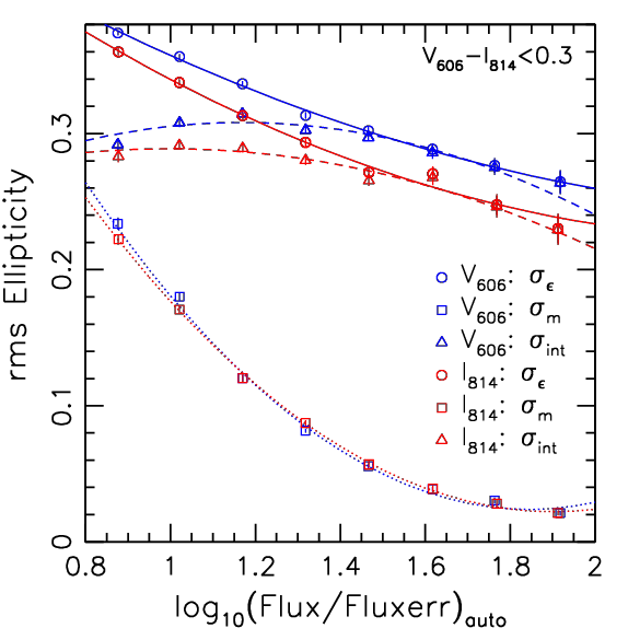
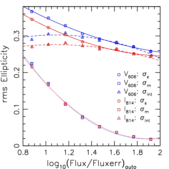
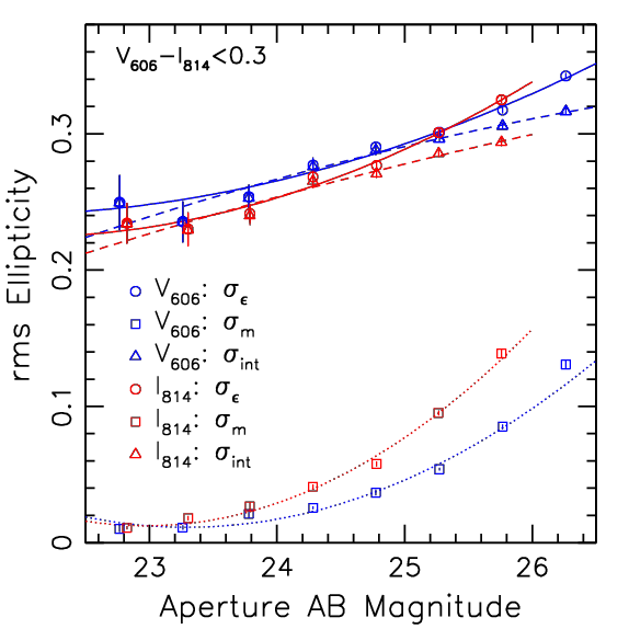
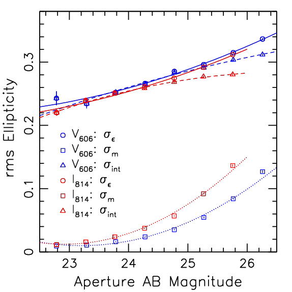
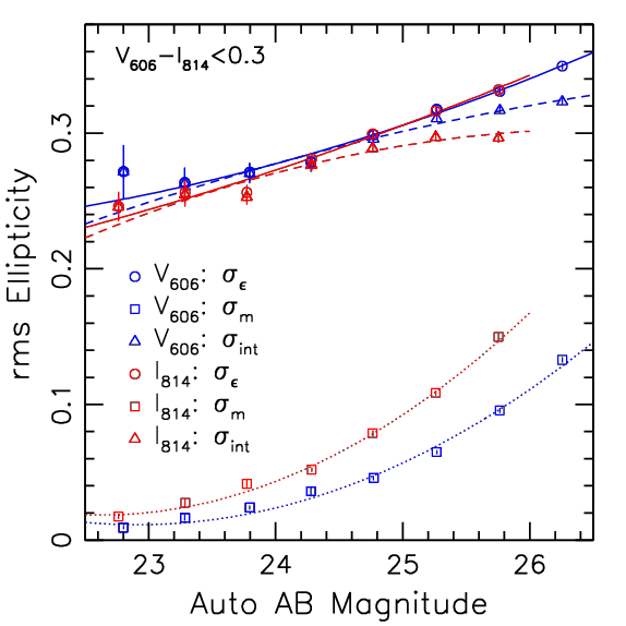
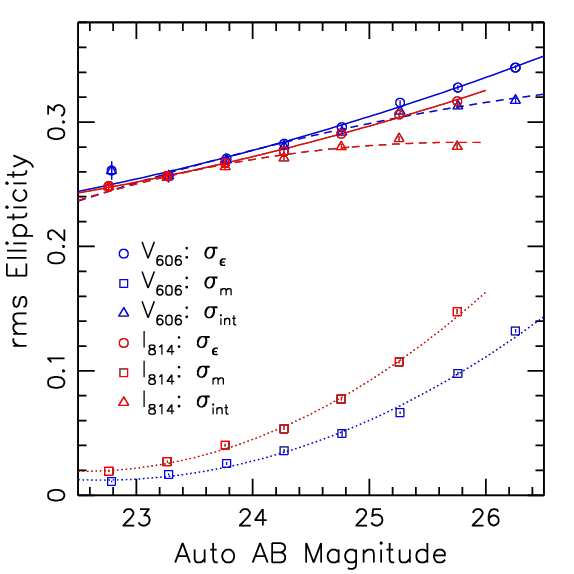
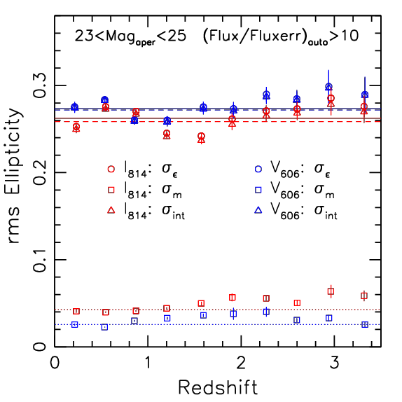
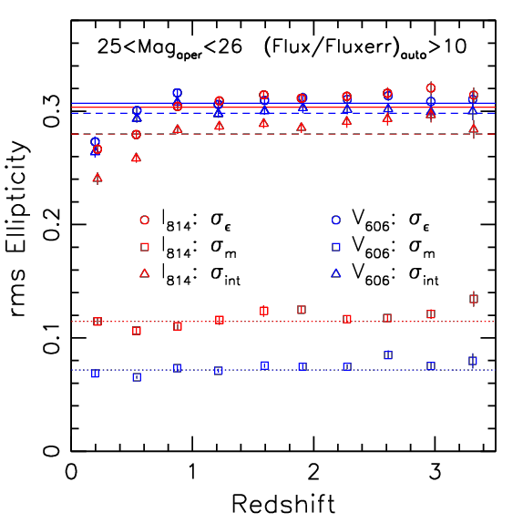
As explained in Section 5 we processed ACS observations in the CANDELS fields to be able to mimic our source selection in the photometric redshift reference catalogues. These blank field data also enable us to study the galaxy ellipticity distribution as detailed in this Appendix. On the one hand this allows us to optimise our weighting scheme for the current study. In addition, these estimates can be used to optimise future weak lensing observing programmes and forecast their performance. For the latter purpose we have studied shape estimates from both ACS standard lensing filters F606W and F814W. This also updates earlier results on the intrinsic ellipticity dispersion estimated by Leauthaud et al. (2007) for F814W observations in the COSMOS Survey.
A.1 Method
Our ellipticity measurements provide estimates for the reduced shear . We model the measured dispersion of the galaxy ellipticity with contributions from the intrinsic galaxy shapes and measurement noise as
| (38) |
The contribution from the cosmological shear in CANDELS is small compared to , and for the purpose of this study we regard it as part of . To estimate we make use of the overlap region of neighbouring ACS tiles (that have similar noise properties), where we have two estimates (a,b) of the ellipticity of each galaxy with two independent realisations of the measurement noise for identical . After rotating the ellipticities to the same coordinate frame, the dispersion of their difference allows us to estimate
| (39) |
from which we compute according to (38). Generally, we quote r.m.s. ellipticity values per ellipticity component, where we compute the average from both components as
| (40) |
A.2 Data
For this analysis we generated and analysed tile-wise F606W and F814W stacks of 4 ACS
exposures each.
We include the initial AEGIS ACS F606W and F814W observations
(Davis et al., 2007, Proposal ID 10134).
Similar to Schrabback et al. (2007)
we generate F606W stacks in GOODS-South and GOODS-North that always combine two
epochs of the observations from Giavalisco et al. (2004, Proposal IDs 9425,
9583). In GOODS-South we also include F606W observations
from GEMS (Rix et al., 2004, Proposal ID
9500), which provides some additional overlap with the S14
WFC3/IR-detected catalogues.
Generally, we limit our analysis to the overlap region with the S14
catalogues to enable the colour selection and provide constraints as
function of photometric redshift.
For the COSMOS and UDS fields we use the F606W and F814W observations from
CANDELS (Grogin et al., 2011, Proposal IDs 12440, 12064). Here, the tile-wise
F606W stacks have slightly shorter integration times of 1.3–1.7 ks compared
to our targeted ks depth.
For the constraints on the ellipticity dispersion we therefore
include these observations
only when studying the ellipticity
dispersion as function of flux signal-to-noise ratio, where the impact of the
shallower depth is minimal.
A.3 Discussion
We plot our estimates for the measured ellipticity dispersion , the intrinsic ellipticity dispersion , and the measurement noise for both ACS filters in Figures 21 to 24.
We investigate the dependencies on the logarithmic flux signal-to-noise ratio , defined via the ratio FLUX_AUTO/FLUXERR_AUTO from SExtractor in Fig. 21, on the aperture magnitude in Fig. 22, and on the auto magnitude from SExtractor in Fig. 23, in all cases with (left panels) and without (right panels) applying our colour selection. As expected, the measurement noise increases steeply towards low signal-to-noise and fainter magnitudes. This is one of the reasons why increases towards lower signal-to-noise and fainter magnitudes. Interestingly, we find that also increases towards fainter magnitudes. The analysis of COSMOS data by Leauthaud et al. (2007) also hinted at this trend with magnitude, but these authors discussed that it might be an artefact from their simplified estimator of the measurement error. We expect that our estimate of the measurement noise from overlapping tiles is fairly robust, and therefore suggest that this indeed appears to be a real effect, showing that intrinsically fainter galaxies have a broader ellipticity distribution.
As a function of the signal-to-noise ratio we largely observe the corresponding trend of an increasing and towards lower , but note that our estimate for flattens at and eventually turns over to decreasing . Using stacks of different depth we verified that this flattening is not intrinsic to the galaxies. Instead, we expect that the validity of Eq. 38 breaks down for large . In addition, selection effects may have some influence, e.g. the cuts applied in size and , as well as non-Gaussian tails in the measured ellipticity distribution at low signal-to-noise.
Comparing the left and right panels in Figures 21 to 23 we find that the application of our colour selection to remove cluster galaxies has only a relatively small impact on the ellipticity dispersion: Applying the colour selection (which preferentially selects blue high- background galaxies) increases by () and by () at magnitudes in the F606W (F814W) filter. This can be compared to the dependence of the ellipticity dispersion on photometric redshift shown in Fig. 24, where we split the sample into bright (left panel) and faint (right panel) galaxies. Over the broad redshift range covered by the HST data the redshift dependence appears to be relatively weak. Most notably, the faint galaxies show an increase in and between redshift 0 and . In principle, one expects such a trend, as galaxies at higher redshifts are observed at bluer rest-frame wavelengths, with stronger light contributions from sites of star formation. However note that it is more challenging to robustly infer conclusions on the redshift dependence of the shape distribution, as this is more strongly affected by large-scale structure variations (compare e.g. Kannawadi, Mandelbaum & Lackner, 2015). We therefore suggest to investigate these trends further in the future with larger data sets.
A.4 Comparing the weak lensing efficiency of F606W and F814W
In Figures 21 to 23 is typically lower for the analysis of the F814W data than for the F606W images at a given signal-to-noise ratio or magnitude. However, when interpreting this one has to keep in mind that the bins do not contain identical sets of galaxies. To facilitate a fair direct comparison of the performance of both filters for weak lensing measurements we limit the analysis to the F606W and F814W AEGIS observations, which were taken under very similar conditions with similar exposure times. As a first test, we compare the ellipticity dispersions computed from those galaxies that have robust shape estimates and in both bands. Including the matched galaxies with we find that on average () is lower for the F814W shape estimates by () compared to the F606W shapes when no colour selection is applied, and by () when blue galaxies are selected with . Hence, we find that intrinsic galaxy shapes are slightly rounder when observed in the redder filter, which reduces their weak lensing shape noise. However, the quantity that actually sets the effective noise level for weak lensing studies is the effective source density after colour selection, which we define as
| (41) |
For a cluster at we find from the AEGIS data that is higher by a factor 1.28 (1.06) for F606W compared to F814W when applying (when not applying) the colour selection with . Hence, if only a single band is observed with HST, F606W is slightly more efficient for the shape measurements than F814W. However, given that the ratio between the estimates is close to unity, we expect that programmes which have observations in both F606W and F814W can achieve a higher effective source density when jointly estimating shapes from both bands. Our work has shown the necessity for depth-matched colours for the cluster member removal. Therefore, we suggest that future HST weak lensing programmes of clusters at should consider to split their observations between F606W and F814W to obtain both colour estimates and joint shape measurements from both bands.
A.5 Fitting functions and shape weights
We compute second-order polynomial interpolations for the ellipticity dispersions as a function of logarithmic signal-to-noise and magnitude within limits as
| (42) |
where . For our weak lensing analysis of SPT clusters we compute empirical shape weights for galaxy as
| (43) |
from the interpolation of as function of the logarithmic signal-to-noise ratio for the colour-selected CANDELS galaxies. We plot the best-fit interpolations in Figures 21 to 23 and list their polynomial coefficients in Table 10.
| Band | Colour | |||||||
|---|---|---|---|---|---|---|---|---|
| all | 0.75 | 2 | ||||||
| all | 0.75 | 2 | ||||||
| all | 0.75 | 2 | ||||||
| all | 22.5 | 26 | ||||||
| all | 22.5 | 26 | ||||||
| all | 22.5 | 26 | ||||||
| all | 22.5 | 26 | ||||||
| all | 22.5 | 26 | ||||||
| all | 22.5 | 26 | ||||||
| 0.75 | 2 | |||||||
| 0.75 | 2 | |||||||
| 0.75 | 2 | |||||||
| 22.5 | 26 | |||||||
| 22.5 | 26 | |||||||
| 22.5 | 26 | |||||||
| 22.5 | 26 | |||||||
| 22.5 | 26 | |||||||
| 22.5 | 26 | |||||||
| all | 0.75 | 2 | ||||||
| all | 0.75 | 2 | ||||||
| all | 0.75 | 2 | ||||||
| all | 22.5 | 26.5 | ||||||
| all | 22.5 | 26.5 | ||||||
| all | 22.5 | 26.5 | ||||||
| all | 22.5 | 26.5 | ||||||
| all | 22.5 | 26.5 | ||||||
| all | 22.5 | 26.5 | ||||||
| 0.75 | 2 | |||||||
| 0.75 | 2 | |||||||
| 0.75 | 2 | |||||||
| 22.5 | 26.5 | |||||||
| 22.5 | 26.5 | |||||||
| 22.5 | 26.5 | |||||||
| 22.5 | 26.5 | |||||||
| 22.5 | 26.5 | |||||||
| 22.5 | 26.5 |
Appendix B Non-matching galaxies in CANDELS
We have investigated the of non-matching galaxies between our CANDELS F606W shear catalogue and the S14 photo- catalogue (see Sect. 6.1) by visually inspecting a random subset. Most of the non-matching galaxies can be explained through differences in the object detection or deblending given the different detection bands (optical F606W vs. NIR F125W+F140W+F160W). For of the total galaxies centroid shifts prevent a match. These should not affect the source redshift distribution. For the S14 catalogue contains a single object which is associated with two deblended objects in our F606W shear catalogue. If such differences in the deblending would occur independent of redshift, there would be no net effect on the source redshift distribution. However, such differences might be more frequent for high- () galaxies, where the F606W images probe rest-frame UV wavelengths and mostly detect sites of star formation, while the IR imaging probes the stellar content of the galaxies. Finally, of the total galaxies show clear isolated galaxies in our F606W shear catalogue that are missing in the S14 NIR-detected catalogue, possibly because they are too faint and too blue.
To obtain a rough estimate for the resulting uncertainty of these effects on our analysis, we assume a scenario where both the missing isolated galaxies () plus the excess half of the differently deblended galaxies () constitute an excess population of 100% blue () galaxies at high redshifts (). This scenario is pessimistic for the differently deblended galaxies as explained above (no impact if the effect is redshift independent). For the missing isolated galaxies the scenario is likely to be realistic, but we note that it would also overestimate the impact in case some of the galaxies are redder and removed by our colour selection. At our median cluster redshift the scenario leads to a relative increase in by only +0.5%, thanks to our colour selection which already selects mostly galaxies.
Appendix C Cross-check for the redshift distribution using spatial cross-correlations
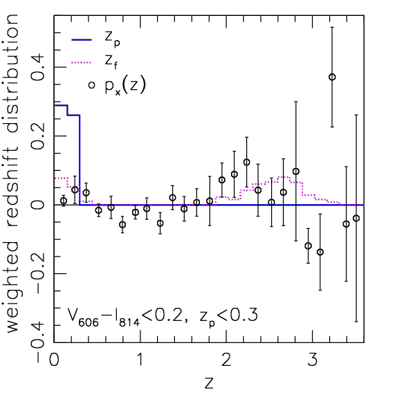
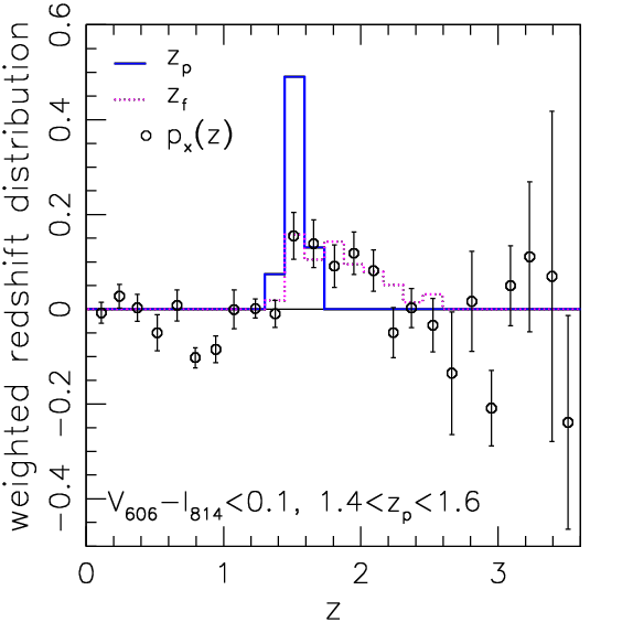
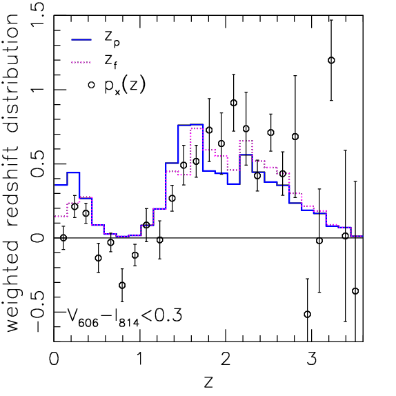
A number of studies have explored the use of spatial cross-correlation techniques to constrain source redshift distributions (e.g. Newman, 2008; Matthews & Newman, 2010; Benjamin et al., 2013). In particular, Newman (2008); Matthews & Newman (2010); Schmidt et al. (2013); Rahman et al. (2015, 2016); Scottez et al. (2016) aim at reconstructing the redshift distribution of a sample with an unknown redshift distribution (“photometric sample”) via its spatial cross-correlation with galaxies in redshift slices of an incomplete spectroscopic reference sample. The cross-correlation amplitude increases if a larger fraction of the photometric sample is located within the redshift range of the corresponding slice. As a result, information on the redshift distribution of the photometric sample can be inferred. When using photometric samples with a broad redshift distribution the accuracy of the method is limited by how well a potential redshift evolution of the relative galaxy bias between the populations can be accounted for (e.g. Rahman et al., 2015). However, the impact of this limitation can be reduced if the photometric sample can be split into sub-samples with relatively narrow individual redshift distributions, as suggested by Schmidt et al. (2013); Ménard et al. (2013) and applied to SDSS data in Rahman et al. (2016). The CANDELS data are well suited to employ this technique, as considerable spectroscopic (or grism) redshift samples are available (Sect. 6.3.3), and given that the 3D-HST photo-s allow for a relatively clean subdivision into narrower redshift slice for most of the galaxies.
We employ the The-wiZZ161616https://github.com/morriscb/The-wiZZ implementation (Morrison et al., 2017) of the cross-correlation technique described in Schmidt et al. (2013); Ménard et al. (2013) to obtain an independent cross-check for our estimate of the colour-selected CANDELS redshift distribution. For this we use the combined sample of high-fidelity spectroscopic and high-quality grism redshifts (see Sect. 6.3.3) as spectroscopic reference sample (without colour selection) and the colour-selected photo- sample as photometric sample, splitting galaxies into 25 linear bins in or , respectively, between and . We compare the estimate for the redshift probability distribution obtained from the cross-correlation analysis using physical separations between 30 kpc and 300 kpc to the and histograms in Fig. 25 using galaxies with and the actual shape weights from our CANDELS shear catalogue.
The left and the middle panels of Fig. 25 correspond to the subset of CANDELS galaxies for which we implemented statistical corrections (see Sect. 6.3) for catastrophic redshift outliers (, ) or redshift focusing (, ), respectively. In both cases we find that the redshift distribution inferred from the cross-correlation analysis is largely consistent with the statistically corrected distribution based on the HUDF analysis (), while it is clearly incompatible with the uncorrected distribution in the selected ranges, providing an independent confirmation for the HUDF-based correction scheme. The right panel of Fig. 25 shows the combined reconstruction for the full colour selected sample (). Consistent with the other panels the reconstruction describes the histogram better than the histogram, both at low redshifts () and around the broad peak at .
The statistical error-bars shown in Fig. 25 indicate the dispersion of the reconstruction when splitting the combined CANDELS data set into 10 subareas of equal area and obtaining 1000 bootstrap resamples of the subareas included in the analysis. We expect that this yields a good approximation for the statistical uncertainty for most of the redshift range of interest. However, at the highest redshifts () the spectroscopic samples become very small (compare Fig. 5), likely introducing additional uncertainties that are not fully captured by the error-bars. This is also suggested by the large fluctuations of both the recovered and the error-bars between neighbouring high- bins.
We note the substantially negative reconstructions at in the middle and right panel of Fig. 25. At these redshifts the full spectroscopic sample contains a large number of galaxies (no colour selection applied to the spectroscopic sample). We therefore expect that the error-bars are robust and that the negative estimates are indeed significant. We interpret these negative values as a spurious effect caused by our colour selection, which explicitly removes galaxies at these redshifts from the photometric sample. Therefore, the photometric sample is spatially underdense in regions that are physically overdense at these redshifts. In contrast, the spectroscopic sample is spatially over-represented in regions of physical overdensities at these redshifts. This results in a net anti-correlation between the samples and negative estimates. As a possible solution to this problem Rahman et al. (2015) suggest to homogenise the spatial density of the spectroscopic sample by removing galaxies in overdense regions. However, as the spectroscopic sample employed in our analysis (14,472 galaxies) is already much smaller than the sample employed by Rahman et al. (2015) (791,546 galaxies) we do not follow this approach. As an approximate solution for this systematic effect we instead set the values of the two bins in Fig. 25 at to zero when computing as described in the next paragraph. This is justified by multiple tests presented in this work that suggest that the residual contamination by galaxies at these redshifts should be very low and close to zero (Sections 6.2, 6.3.3, 6.4, 6.8). However, outside this redshift range we treat bins with negative as negative contributions in the computation of . This is needed in order to achieve unbiased results in the case of purely statistical scatter that has equal chance to be positive or negative.
For a quantitative comparison of the distribution and the histograms shown in the right panel of Fig. 25 we compute for our median cluster redshift , dealing with negative as explained in the previous paragraph, and generally limiting the considered redshift range to to minimise the impact of the highest- data points for which the recovery suffers the strongest from the small spectroscopic sample. The resulting from the cross-correlation analysis (the error indicates the statistical scatter from the bootstrap resamples) is consistent with from the HUDF-corrected catalogues within . We conclude that the cross-correlation analysis independently supports the results from the HUDF analysis, but note that the spectroscopic samples within the relatively small CANDELS areas are not yet sufficiently large to constrain the redshift distribution with very high precision.
Appendix D Details of the ACS+FORS2 colour measurements and the accounting for photometric scatter
D.1 ACS+FORS2 colour measurement
To measure colours between the F606W and FORS2 I-band images images we convolve each mosaic F606W image with a Gaussian kernel such that the resulting PSF has the same FLUX_RADIUS measured by Source Extractor as the corresponding FORS2 I-band image (we empirically account for the impact of non-Gaussian VLT PSF profiles in Appendix D.2). For some of the FORS2 stacks we found small residual systematic offsets of object positions in some image regions with respect to their location in the corresponding ACS mosaic (typically ). To not bias the colour measurement, we therefore fit and subtract a smooth 5th-order 2D-polynomial interpolation of the measured positional offsets to the catalogue positions. We overlayed and visually inspected these corrections on all images to ensure that they are robust. We then measure object fluxes in circular apertures with diameter 15 both in the VLT and the convolved ACS image. We transform them into magnitudes, correct these for galactic extinction, and compute the colour estimate .
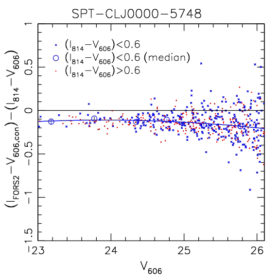
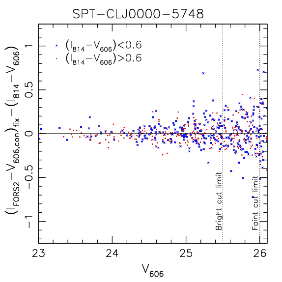
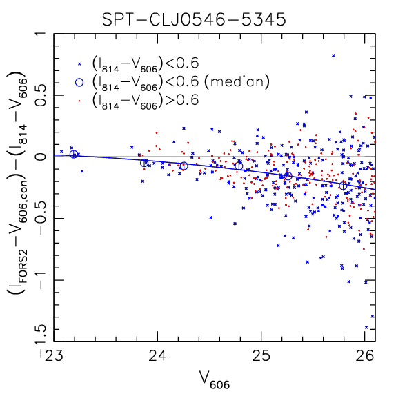
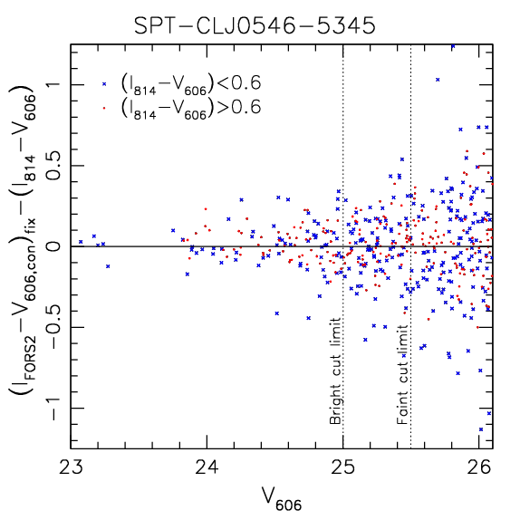
D.2 Tying the ACS+FORS2 colours to the ACS-only colours
We have ACS-based and ACS+FORS2-based colour estimates for the galaxies in the inner cluster regions. We use these galaxies to refine the calibration of the colours for all galaxies and tie them to the colour selection available in the 3D-HST CANDELS catalogues. The left panels of Fig. 26 shows the difference of these colour estimates as function of for two example clusters. The top row corresponds to SPT-CL 00005748, which has one of the deepest and best-seeing FORS2 I-band stacks in our sample, resulting in relatively moderate photometric scatter. Here the analysis reveals a mag colour offset for bright galaxies. We expect that this offset is in part caused by the offset in Eq. (16). Further contributions might come from uncertainties in the zero-point calibration due to the small number of stars available for its determination, or inaccuracies in the PSF homogenisation. In comparison, the bottom row reveals a larger photometric scatter for SPT-CL 05465345, which has a shallower magnitude limit and worse image quality (see Table 2). For such VLT data we typically detect a shift of the median colour difference (indicated through the open circles) at faint magnitudes towards negative values. In part this is caused by the asymmetric and biased scatter in logarithmic magnitude space. However, further effects could lead to a magnitude-dependent colour offset: for example, we acknowledge that our PSF homogenisation only ensures equal flux radii between the bands. However, residual differences in the actual PSF shapes might lead to slightly different fractions in the total PSF flux lost outside the aperture. This would lead to a magnitude-dependent colour offset given that fainter objects are typically less resolved. Understanding the exact combination of these effects for each cluster is not necessary given that we directly tie the colours to the colours empirically: To do so, we fit the median values of the colour offsets determined in 0.5 mag-wide bins between with a second order polynomial in and subtract this model from all colour estimates in the cluster field to obtain (see Fig. 26). We only use relatively blue galaxies with to derive this fit. This is motivated by small differences in the effective filter curves of and . In particular, cuts off transmission red-wards of nm, while has a transmission tail out to nm. Thus, we expect non-negligible colour differences for very red objects. Given that we generally apply fairly blue cuts in colour this is not a problem for our analysis. However, we exclude red galaxies when deriving the fit as they are over-represented compared to CANDELS in the cluster fields.
D.3 Accounting for photometric scatter
D.3.1 ACS-only colour selection
In the inner cluster regions covered by the F606W and F814W ACS images we include galaxies in the magnitude range . The brighter magnitude limit has been chosen as galaxies passing our colour selection at even brighter magnitudes are dominated by foreground galaxies. The fainter magnitude limit approximately matches the cut applied in the weak lensing shape analysis (see Sect. 5). Our ACS images have typical limits for the adopted 07 apertures of and . Therefore, the faintest galaxies included at the colour cut (, ) still have fairly high photometric signal-to-noise and . Accordingly, photometric noise has only minor impact on the colour selection for these galaxies. Nonetheless, we account for it by adding random Gaussian scatter to the S14 catalogues, which are typically based on deeper ACS mosaic stacks compared to the ones used for our shape analysis, prior to the colour selection, such that they have the same limiting magnitudes in and as our cluster field observations. Also, we apply a slightly bluer colour selection for the galaxies in the faintest magnitude bin (see Table 11 and Sect. 6.2).
| bright | faint | |||
|---|---|---|---|---|
| 0.3 | 0.2 | 0.2 | 0.0 | |
| 0.2 | 0.1 | 0.1 | ||
Note. — Colour cut limits applied in our analysis. Column 1: Cluster redshift range. Column 2: Colour-cut in ACS-only colour for galaxies with . Column 3: Colour-cut in ACS-only colour for galaxies with . Column 4: Colour cut in the ACS+FORS2 colour after tying it to the colour (see Appendix D.2), as employed for “bright cut” magnitude bins with low photometric scatter . Column 5: As column 4, but for the “faint cut” magnitude bins with increased photometric scatter .
D.3.2 ACS+FORS2 colour selection
The colour estimates that include the FORS2 data are more strongly affected by photometric scatter than the colours obtained from the high-resolution ACS data only (see Fig. 26). To ensure that we can still apply a consistent colour selection to the S14 catalogues we do the following:
First, we limit the analysis to relatively bright magnitudes, to ensure that the scatter is small enough to not compromise the exclusion of galaxies at the cluster redshift considerably. For this we compute the r.m.s. scatter in the colour difference of blue galaxies () in 0.5 mag-wide bins in . For the ACS+FORS2 colour selection we only include magnitudes bins with scatter . Here we employ our standard (“bright”) colour cut for the magnitude bins with low scatter , and a more conservative (“faint”) colour cut for magnitude bins with slightly larger scatter , see columns 5 and 6 in Table 2 for the corresponding magnitude bins in each cluster and Table 11 for the colour cuts as function of cluster redshift.
Second, we add noise to the colour estimates in the CANDELS catalogue prior to the colour cut, similarly to our approach for the ACS-only selection. However, in contrast to Appendix D.3.1 we do not assume a Gaussian noise distribution here, but randomly sample the noise from the actual distribution of the colour differences shown in the right panels of Fig. 26. The motivation for not using a Gaussian approximation is given by the skewness in the distribution and presence of outliers. In practice, we again divide the galaxies into 0.5 mag-wide bins in . We further subdivide these galaxies into sub-bins according to their colour if sufficiently many galaxies are available to provide sub-bins containing at least 30 galaxies each. For each galaxy in the CANDELS catalogue we then identify the corresponding bin/sub-bin and randomly assign a colour difference drawn from this bin/sub-bin. Note that we introduce the further colour subdivision as red galaxies (which are later removed by the colour cut) show a lower scatter at a given magnitude171717This is expected since receives roughly comparable scatter contributions from and , with a reduced scatter in for red objects..
Appendix E Limitations of a statistical correction for cluster member contamination
Weak lensing studies that use wide-field imaging data and do not have sufficient colour information for a robust removal of cluster galaxies can attempt to statistically correct their shear profiles for the dilution effect of cluster members in the source samples (see e.g. Hoekstra et al., 2015). For this, they need to estimate the relative excess counts as function of cluster-centric distance, ideally accounting for the impact of masks, obscuration by cluster members, and magnification, and fit it with a model, typically in the form
| (44) |
and scale the shear profile as
| (45) |
Here we consider two previously employed models for the projected density profiles of cluster galaxies, namely the projected singular isothermal sphere (SIS) model
| (46) |
(e.g. Hoekstra, 2007) and an exponential model
| (47) |
(e.g. Applegate et al., 2014), where corresponds to the contamination at .
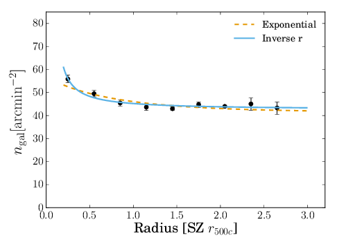
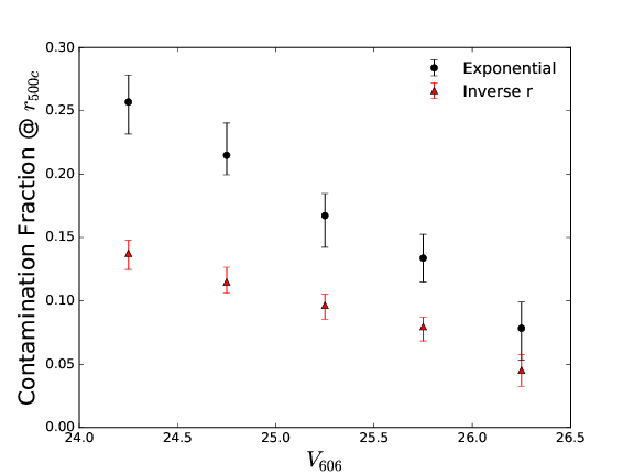
We do not use this approach for our HST analysis as the ACS mosaics are too small to derive a robust estimate of the background source density directly. To test this, we use our source catalogues without colour selection, estimate the mask- and obscuration-corrected source density profiles in magnitude bins, and fit them with both profiles. Combining the analysis from all clusters we find that both profiles provide acceptable fits for most of the radial range covered by the ACS data. For example, when using only a single broad magnitude bin, the SIS model returns for 7 degrees of freedom, whereas the exponential model returns . The SIS model is clearly a better fit at small radii (see the left panel of Fig. 27), but the exponential profile is not ruled out at high significance. Yet, the two models yield uncomfortably different contamination fractions (shown in the right panel of Fig. 27 as function of ). As a test for the impact of these differences we artificially apply the two different boost correction schemes (taking their magnitude dependencies into account) to our colour-selected shear profiles and compare the resulting mass estimates. Here we find that the exponential model leads to mass estimates which are higher compared to those from the isothermal model by . As it is currently not clear what the correct functional form would be, we conclude that the application of such a contamination correction would introduce substantial systematic uncertainty.
One could consider to reduce this uncertainty by using external blank fields to constrain the background source density. Using our colour-selected catalogues we have demonstrated that the careful matching of source selection criteria and noise properties between the cluster and reference fields, which would be required for such an approach, is in principle possible. However, instead of providing an important validation test as in our study, the information in the number density would then be used to correct the signal, assuming that all other related analyses steps were done correctly. Large-scale structure variations also introduce significant variations in the source densities between the five CANDELS fields. Without colour selection we find that they lead to uncertainties in the estimated mean background density of at to at .
In addition to the increased systematic uncertainty, the use of a contamination correction also increases the statistical uncertainty compared to a robust colour selection that adequately removes cluster galaxies. First, the cluster members dilute the small-scale signal, which is the regime providing the highest signal-to-noise contribution for our analysis. Second, source density profiles are typically too noisy to measure the contamination for individual clusters. On the other hand, if an average contamination model is applied, extra scatter in the mass constraints is introduced.
Appendix F Impact of contamination by very blue cluster members
The tests presented in Sect. 6.8 show no indication for a significant residual contamination by cluster members. However, our estimates from Sect. 6.4 suggest that, in the presence of noise and averaged over our cluster sample, our ACS-only (ACS+FORS2) colour selection should leave a residual contamination of () of very blue field galaxies at the corresponding cluster redshifts. Whether or not this can introduce a residual excess contamination by cluster members depends on the relative properties of the galaxy distributions in the field and cluster environment.
Luminous Compact Blue Galaxies (LCBGs, e.g. Koo et al., 1994) represent an extreme star-bursting population of galaxies with very blue colours and compact sizes. Such galaxies were also identified in cluster environments (Koo et al., 1997), making them the most relevant potential contaminant for our colour-selected weak lensing source sample. Crawford et al. (2011); Crawford, Wirth & Bershady (2014) and Crawford et al. (2016) identify and study LCBGs in five massive clusters at using a photometric preselection, Keck/DEIMOS spectroscopy, and HST morphological measurements. For the clusters in their sample Crawford et al. (2011) find that the number density enhancement of the cluster LCBG population compared to the LCBG field density is comparable to or lower than the corresponding enhancement of the total cluster population compared to the total field population. In addition, Crawford et al. (2016) find that the relevant properties of the cluster LCBGs (star-formation rate, dynamical mass, size, luminosity, and metallicity) are indistinguishable from the properties of field LCBGs at the same redshift.
Accordingly, we can make the conservative assumption that the relative fraction of cluster members that pass our colour selection is equal to or lower than the fraction of field galaxies passing the selection for the ACS-only (ACS+FORS2) selection, accounting for noise (see Sect. 6.4). We then estimate the approximately expected average fraction of cluster galaxies in our colour-selected source sample at as
where indicates an estimate for the average contamination at based on a number density profile analysis when the colour selection is not applied (see the right panel of Fig. 27, averaging the values for the more conservative exponential model according to the relative weight of the corresponding magnitude bin in the reduced shear profile fits), and corresponds to the fraction of galaxies in the cluster fields passing the colour selection within the magnitude range of the ACS-only (ACS+FORS2) analysis. We do not attempt to model the radial distribution of the expected contaminating cluster galaxies, as LCBGs appear to follow a rather shell-like distribution with a depletion in the cluster core (Crawford et al., 2006). Instead, we assume that provides a reasonable approximation for the typical contamination, which is likely conservative given that the average kpc of our cluster sample (based on the lensing analysis and assuming the concentration–mass relation from Diemer & Kravtsov, 2015, see Sect. 7) is more representative for the inner ( kpc) than the outer ( Mpc) limit of the fit range for our default analysis. With these conservative assumptions, the relative bias for the average lensing efficiency caused by the expected cluster contamination is . Given that this is even smaller than the uncertainty on from line-of-sight variations between the CANDELS fields (Sect. 6.6), this bias could well be ignored (we still include it in the systematic error budget in Table 8). But we note that future studies could attempt to model the contamination more accurately and apply a correction.
Appendix G Additional figures
Figures 28 to 39 complement Fig. 14 and Fig. 16, showing the corresponding results for the other clusters. In particular, the left and middle panels show the weak lensing mass reconstructions overlaid onto the corresponding VLT/FORS2 and central ACS colour images, as well as the locations of the different cluster centres used in our analysis. In the corresponding right panels we show the weak lensing shear profiles centred onto the X-ray centroids.
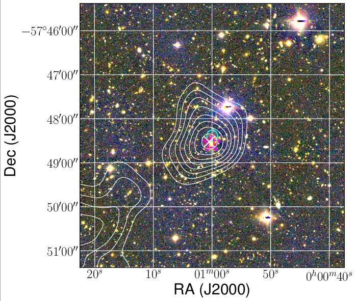
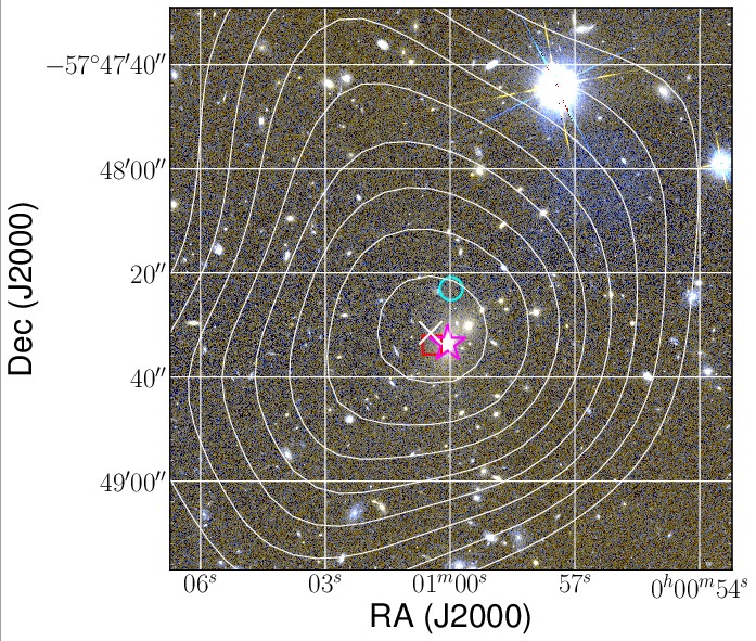
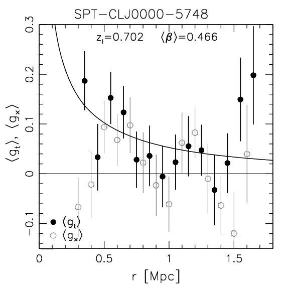
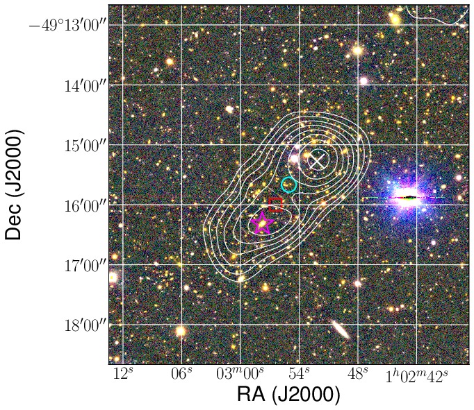
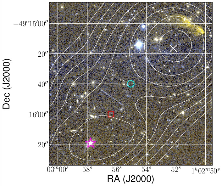
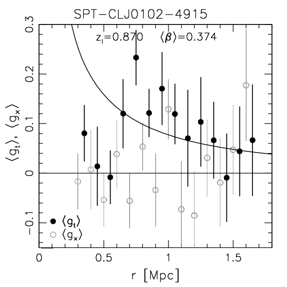
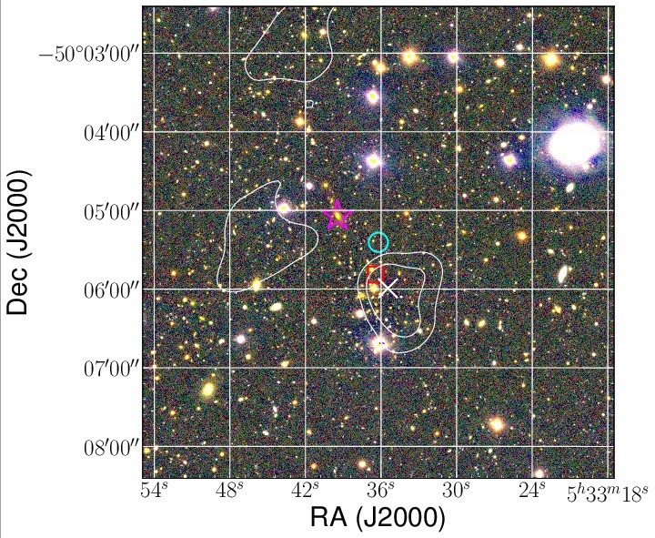
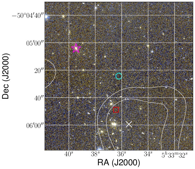
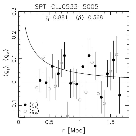
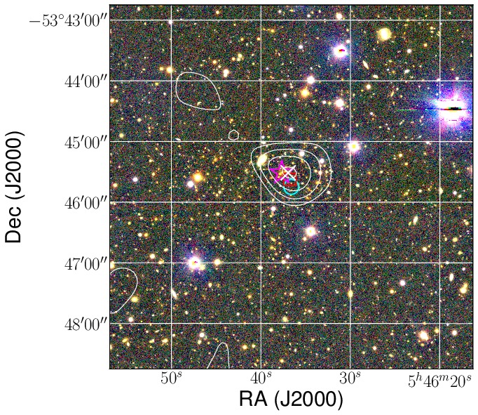
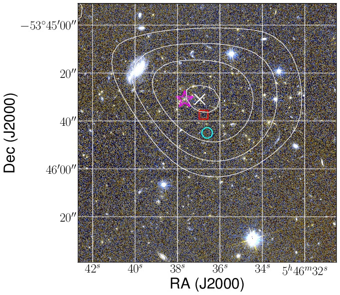
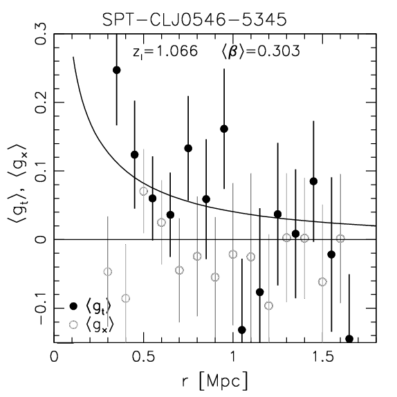
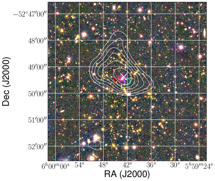
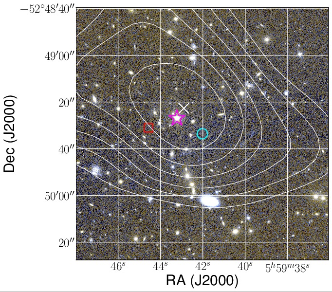
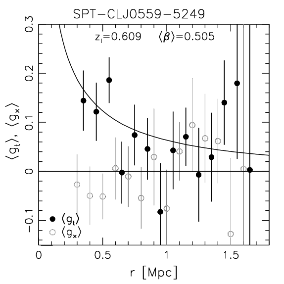
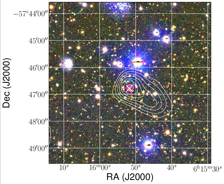
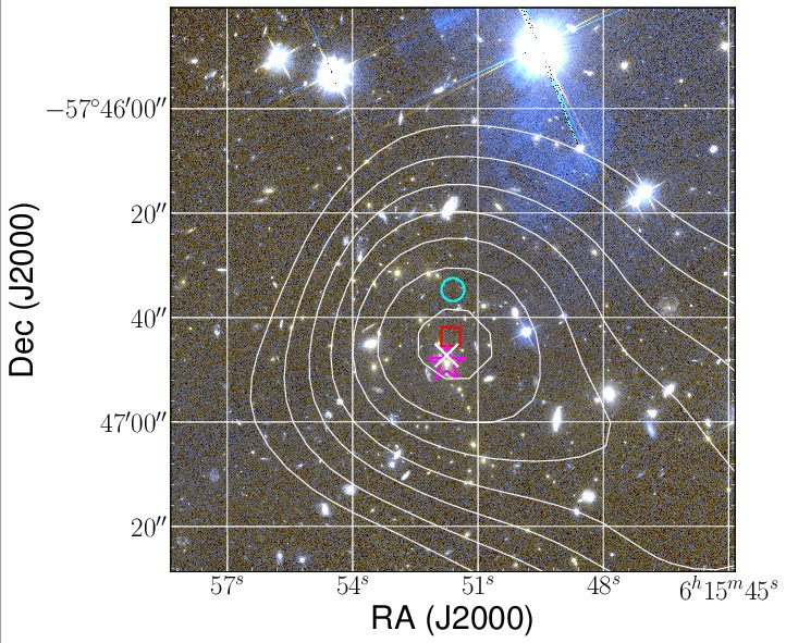
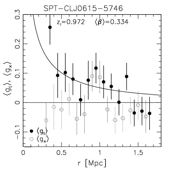
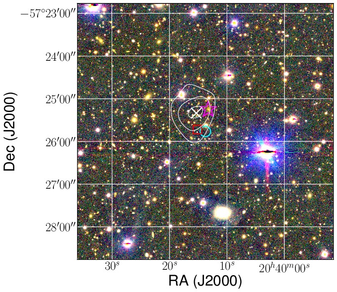
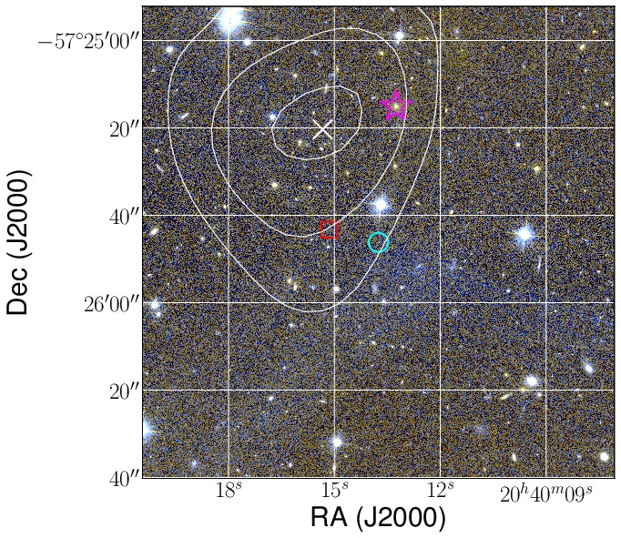
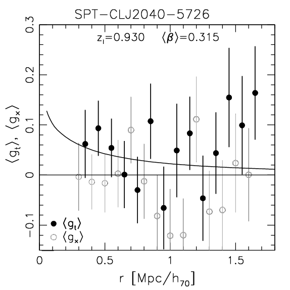
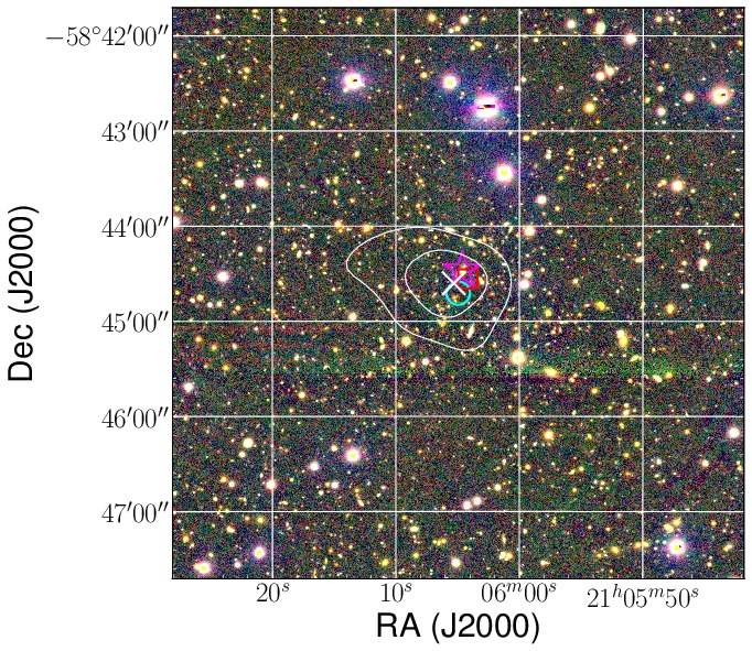
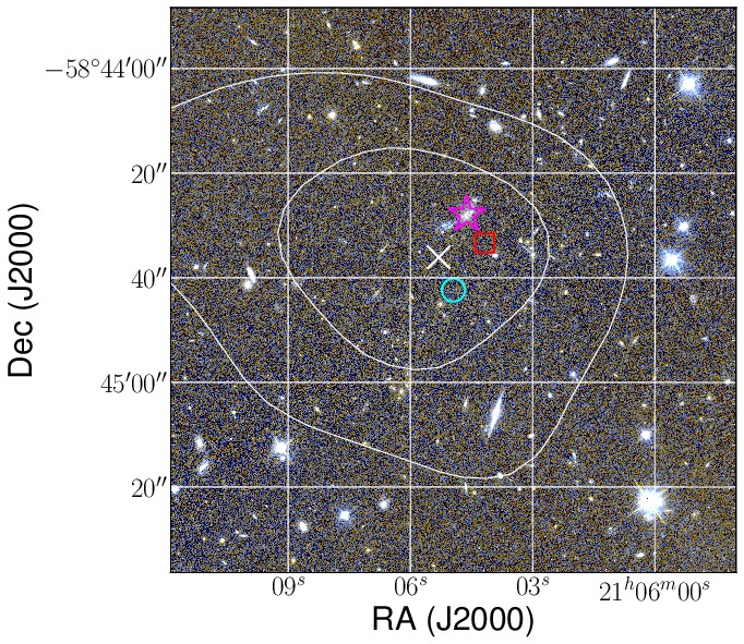
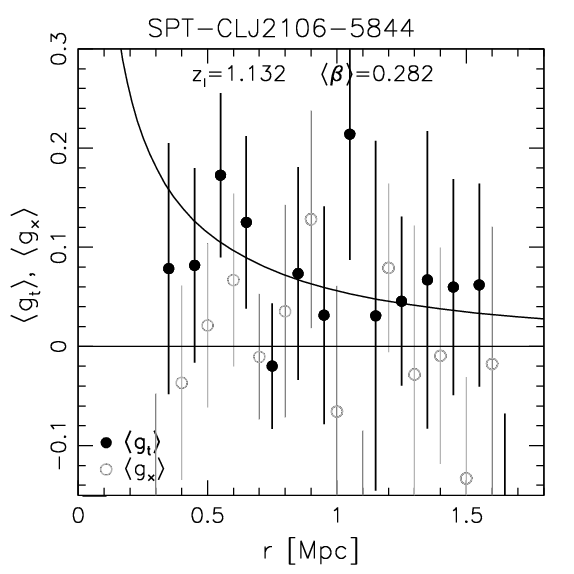
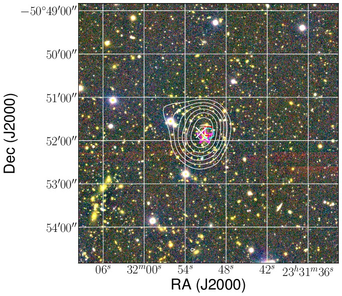
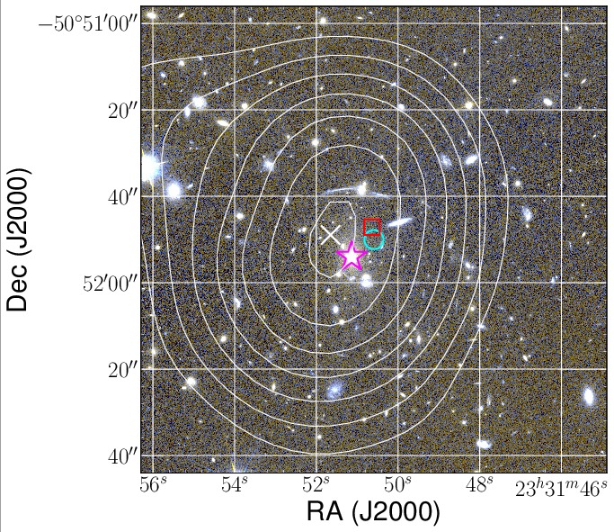
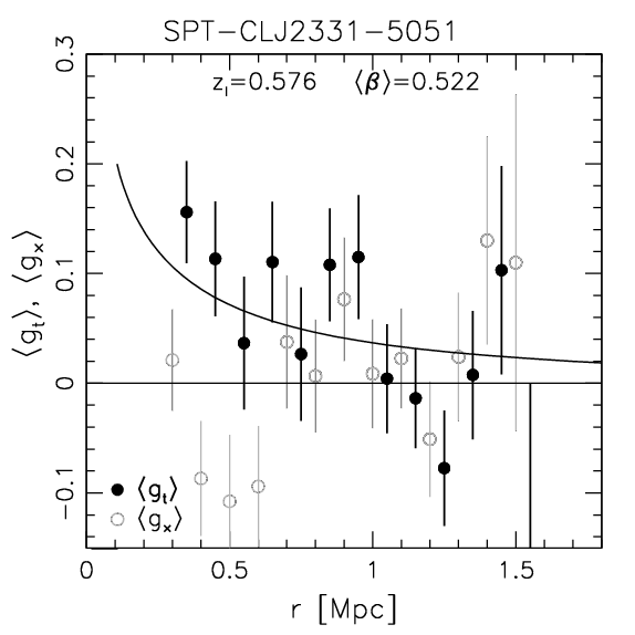
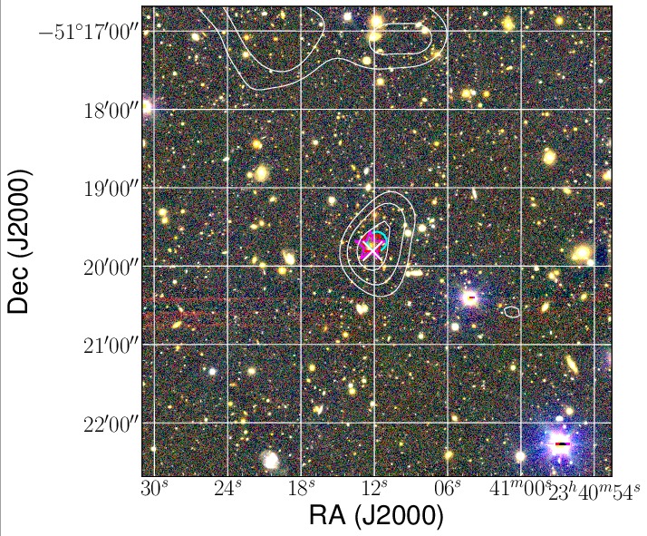
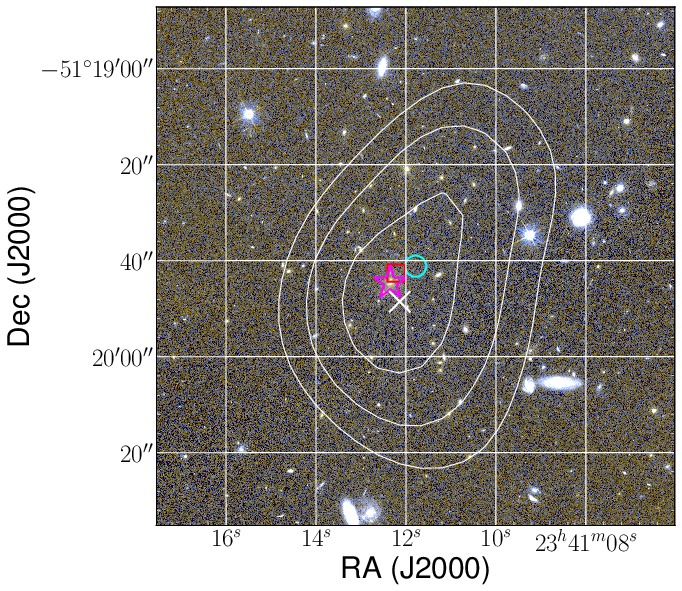
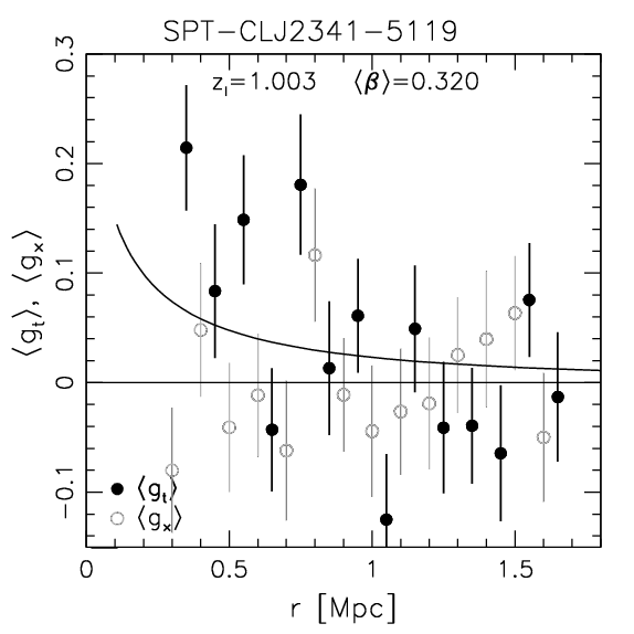
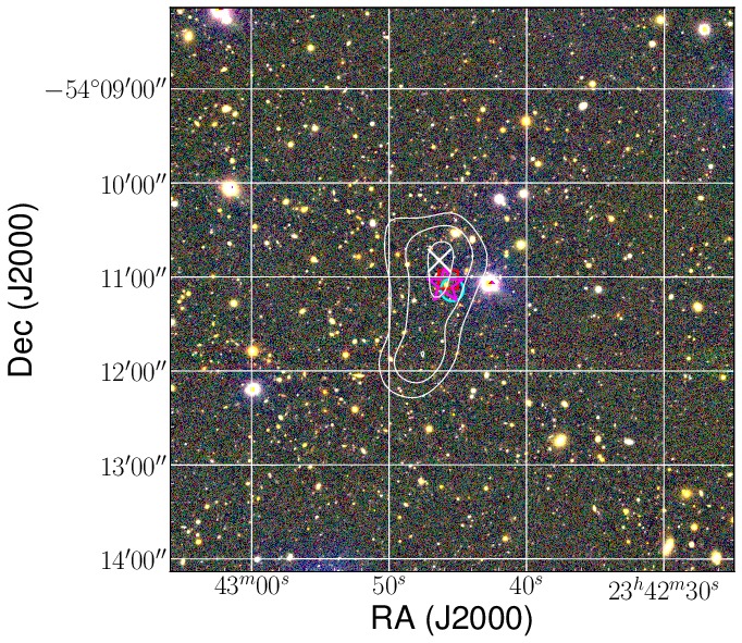
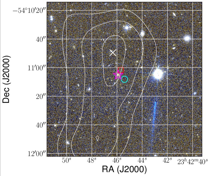
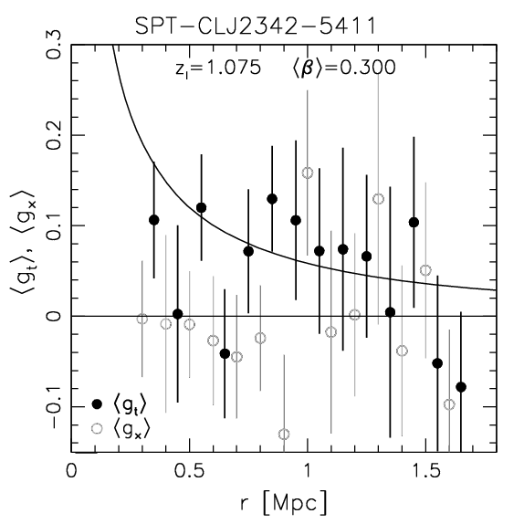
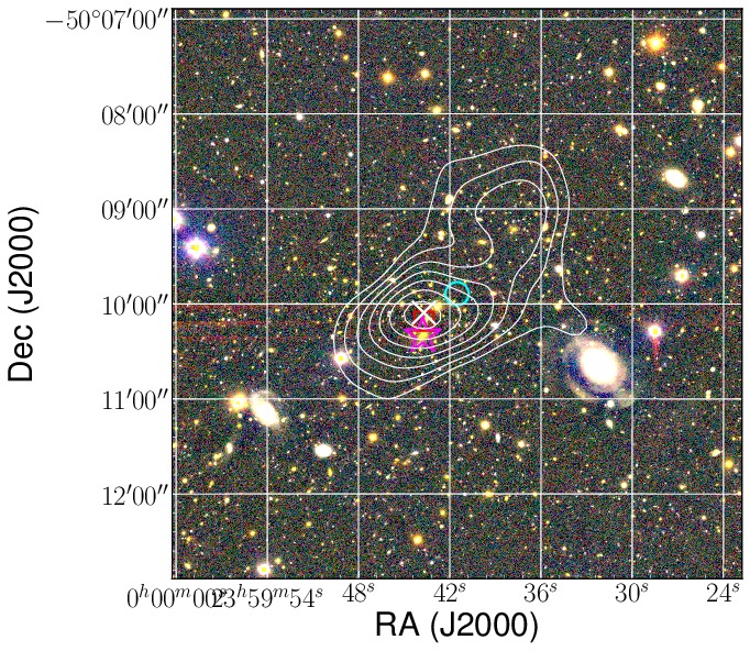
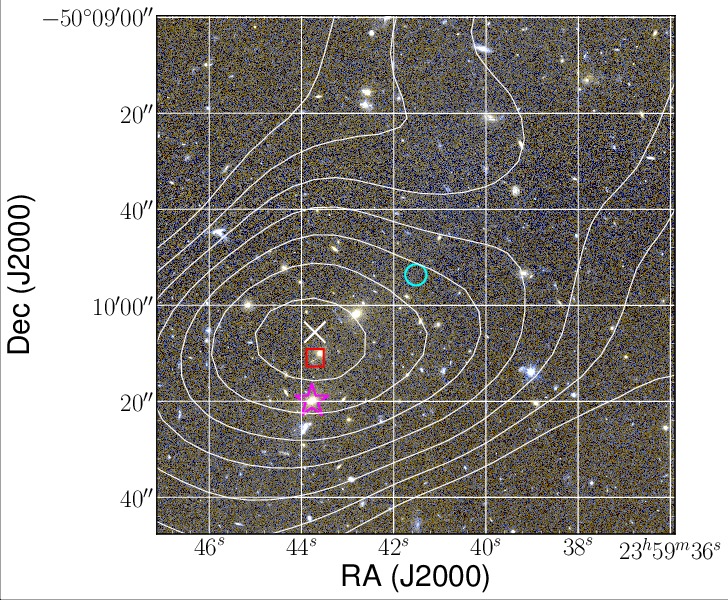
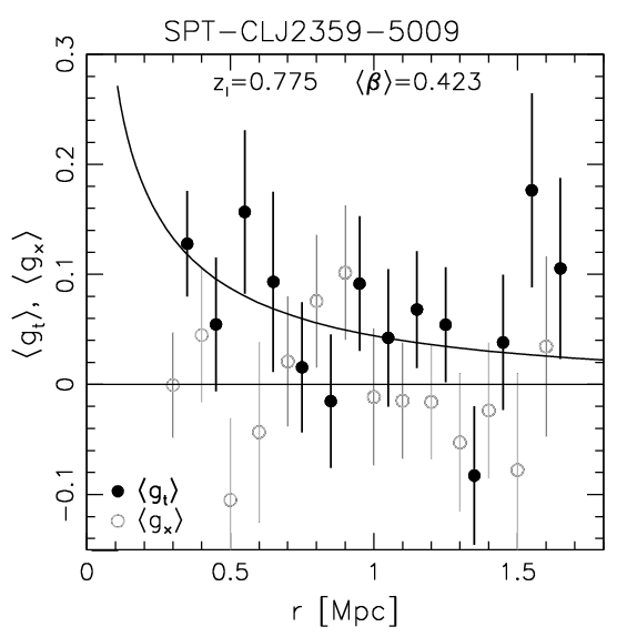
Affiliations
1 Argelander-Institut für Astronomie, Universität Bonn, Auf dem
Hügel 71, 53121, Bonn, Germany
2 Kavli Institute for Particle Astrophysics and
Cosmology, Stanford University, 382 Via Pueblo Mall, Stanford, CA
94305-4060, USA
3 Department of Physics, Stanford University, 382 Via Pueblo Mall, Stanford,
CA 94305-4060, USA
4 Kavli Institute for Cosmological Physics, University of Chicago, 5640 South Ellis Avenue, Chicago, IL 60637
5 Faculty of Physics, Ludwig-Maximilians University, Scheinerstr. 1, 81679 München, Germany
6 Excellence Cluster Universe,
Boltzmannstr. 2, 85748 Garching, Germany
7 Leiden Observatory, Leiden University, Niels Bohrweg
2, NL-2300 CA Leiden, The Netherlands
8 Argonne National Laboratory, 9700 S. Cass Avenue,
Argonne, IL, USA 60439
9 Department of Astronomy, University of Florida,
Gainesville, FL 3261
10 Dark Cosmology Centre, Niels Bohr Institute,
University of Copenhagen, Juliane Maries Vej 30, DK-2100 Copenhagen,
Denmark
11 Department of Physics and Astronomy, Stony Brook University, Stony Brook, NY 11794, USA
12 MIT Kavli Institute for Astrophysics and Space
Research, Massachusetts Institute of Technology, 77 Massachusetts
Avenue, Cambridge, MA 02139
13 Department of Astronomy, University of Washington, Box 351580, Seattle, WA 98195, USA
14 SLAC National Accelerator Laboratory, 2575 Sand Hill Road, Menlo Park, CA 94025, USA
15 Department of Physics, Harvard University, 17 Oxford Street, Cambridge, MA 02138
16 Harvard-Smithsonian Center for Astrophysics,
60 Garden Street, Cambridge, MA 02138
17Department of Physics & Astronomy, Colby College,
5800 Mayflower Hill, Waterville, Maine 04901
18Fermi National Accelerator Laboratory, Batavia, IL 60510-0500, USA
19 Department of Astronomy and Astrophysics, University of Chicago, 5640 South Ellis Avenue, Chicago, IL 60637
20 Department of Physics, University of Chicago,
5640 South Ellis Avenue, Chicago, IL 60637
21 Academia Sinica Institute of Astronomy and Astrophysics (ASIAA)
11F of AS/NTU Astronomy-Mathematics Building,
No.1, Sec. 4, Roosevelt Rd, Taipei 10617, Taiwan
22 Department of Physics, IIT Hyderabad, Kandi, Telangana 502285, India
23 Department of Astronomy and Astrophysics, University of California, Santa Cruz, CA 95064, USA
24 Department of Physics, McGill University, 3600 Rue
University, Montreal, Quebec H3A 2T8, Canada
25 Department of Physics, University of California,
Berkeley, CA 94720
26 Institute for Computational Cosmology, Durham University, South Road, Durham DH1 3LE, UK
27 Max Planck Institute for Extraterrestrial Physics,
Giessenbachstrasse 1, 85748 Garching, Germany
28 School of Physics, University of Melbourne, Parkville, VIC
3010, Australia
29 Cerro Tololo Inter-American Observatory, Casilla 603, La Serena, Chile