Linking the x3d pathway to integral field spectrographs:
YSNR 1E 0102.2-7219 in the SMC as a case study

Abstract

The concept of the x3d pathway was introduced by Vogt et al. (2016) as a new approach to sharing and publishing 3-D structures interactively in online scientific journals. The core characteristics of the x3d pathway are that: 1) it does not rely on specific software, but rather a file format (x3d), 2) it can be implemented using fully open-source tools, and 3) article readers can access the interactive models using most main stream web browsers without the need for any additional plugins. In this article, we further demonstrate the potential of the x3d pathway to visualize datasets from optical integral field spectrographs. We use recent observations of the oxygen-rich young supernova remnant 1E 0102.2-7219 in the Small Magellanic Cloud to implement additional x3dom tools & techniques and expand the range of interactions that can be offered to article readers. In particular, we present a set of javascript functions allowing the creation and interactive handling of clip planes, effectively allowing users to take measurements of distances and angles directly from the interactive model itself.

1. Introduction

Oxygen-rich (O-rich) young supernova remnants (YSNRs) form a special subclass of supernova remnants (SNRs). In those systems, the observed forbidden-line oxygen emission is understood to arise from ejecta encountering (at several 1000 km s^-1) the reverse shock wave from a type Ib supernova that had been stripped of its hydrogen envelope prior to the explosion (Sutherland & Dopita, 1995). O-rich YSNRs are as such unlike most SNRs where the optical emission comes from the interstellar medium ionized by the forward shock. Only a handful of such O-rich YSNRs are known: these include Cas A (Chevalier & Kirshner, 1979), G292.0+1.8 (Goss et al., 1979; Murdin & Clark, 1979) and Puppis A (Winkler & Kirshner, 1985) in our Galaxy, N132D (Danziger & Dennefeld, 1976b, a; Lasker, 1978) & SNR 0540-69.3 (Mathewson et al., 1980) in the Large Magellanic Cloud, and 0103-72.6 (Park et al., 2003), B0049-73.6 (Hendrick et al., 2005; Schenck et al., 2014) & 1E 0102.2-7219 (1E 0102 for short; Dopita et al., 1981; Tuohy & Dopita, 1983) in the Small Magellanic Cloud (SMC).

The ages of O-rich YSNRs are typically only of a few thousands of years, so that the O-bright ejecta have not (yet) had time to strongly interact with the surrounding medium. It is thus reasonable to assume that the ejecta have been freely expanding since the time of the SN explosion (see e.g. Milisavljevic & Fesen, 2013). This property can be used to derive the ages of YSNRs through the measurement of their ejecta’s proper motion, which display typical velocities of the order of several $1000$ km s^-1 (van den Bergh & Dodd, 1970; Thorstensen et al., 2001; Fesen et al., 2006; Finkelstein et al., 2006; Winkler et al., 2009).

When observed with integral field spectrographs (IFS), the free expansion assumption allows the reconstruction of the full three-dimensional (3-D) spatial distribution of the O-rich ejecta in space. Provided that the age of the YSNR is known (e.g. through proper motion measurements and/or from historical records), the ejecta radial velocities (measured through Doppler shifts) can be trivially transformed into physical distances along the line of sight $z$ using the relation:

$$z=v_{los}\Delta t$$ (1)

with $\Delta t$ the time since the SN explosion and $v_{los}$ the line-of-sight velocity of the ejecta. Assuming that the distance to the YSNR is also known, angular separations on-sky can be transformed into physical distances, thus leading to the full 3-D localization of the ejecta in space. Vogt & Dopita (2010) and Vogt & Dopita (2011) applied this technique to YSNR 1E 0102 and N132D, respectively. Milisavljevic & Fesen (2013) used a similar approach (using numerous long-slit observations) to reconstruct the 3-D map of the ejecta in Cas A.

In this article, we exploit new IFS observations of YSNR 1E 0102 to link the concept of the x3d pathway to data products from integral field spectrographs. The x3d pathway was first implemented by Vogt et al. (2014) and formally defined by Vogt et al. (2016) as a new way to share and publish 3-D astrophysical models interactively. The x3d pathway revolves around the x3d file format and the associated x3dom (pronounced X-Freedom) framework to share 3-D models on the World Wide Web. Here, we use 1E 0102 to complement the examples of Vogt et al. (2016) that applied the x3d pathway to H I observations of a compact group of galaxies observed with the Very Large Array. The very nature of YSNR 1E 0102, and in particular the ability to reconstruct the 3-D map of its O-rich ejecta, effectively makes it the ideal candidate for demonstrating the potential of the x3d pathway when coupled to optical IFS datasets. Another implementation of the x3d pathway applied to the MUSE IFS observation of an extragalactic target is to be presented by Bellhouse et al. (in prep).

After introducing our IFS observations of YSNR 1E 0102 in Sec. 2, we describe our interactive 3-D map of the O-rich ejecta in this system in Sec. 3, and introduce new x3dom-based tools to interact with 3-D models in Sec. 4. We summarize our conclusions in Sec. 5.

2. Revisiting YSNR 1E 0102 with WiFeS

YSNR 1E 0102 was observed with the WiFeS IFS (Dopita et al., 2007, 2010) – mounted on the 2.3m Advanced Technology Telescope (ATT) of the Australian National University at Siding Spring Observatory (NSW, Australia; Mathewson et al., 2013) – in 2016, August as part of a series of observations of SNRs in both the SMC and LMC (P.I.: Seitenzahl). YSNR 1E 0102 had already been observed with WiFeS in late 2009 (P.I.: Dopita): that dataset then led to the first 3-D reconstruction of the O-rich ejecta in this system (Vogt & Dopita, 2010). The most recent WiFeS observations of YSNR 1E 0102 improved on the 2009 observations as follows: 1) they were performed using the second generations of CCDs in the WiFeS instrument, 2) the resulting 4-fields WiFeS mosaic does not contain any gap, and 3) the data were reduced using the pywifes data reduction pipeline (Childress et al., 2014a, b). The observation details and scientific implication of this new dataset are to be described in Seitenzahl et al. (in prep.). For the purpose of this article, it is sufficient to say that the 2016 WiFeS mosaics of YSNR 1E 0102 is composed of 4 overlapping WiFeS fields (each of 25$\times$38 square arcsec with $1\times 1$ square arcsec spatial pixels or spaxels) with a total size of $56\times 48$ square arcsec. The dataset is comprised of two mosaics (the red and the blue): a structure inherent of the dual-beam design of the spectrograph.

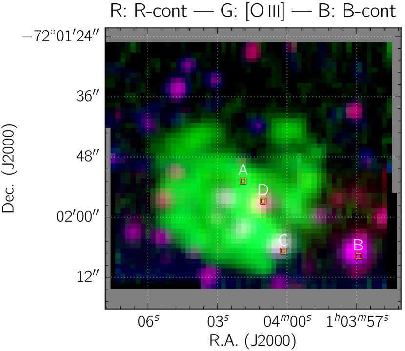
In this work, we solely focus on the blue mosaic unless explicitly mentioned otherwise. The observations were performed with the B7000 grating for the blue arm, resulting in a spectral resolution of R=7000 and a spectral coverage ranging from 4200 Å to 5548 Å. The seeing during the observations was of the order of 1.5 arcsec. A pseudo-RGB image of YSNR 1E 0102 highlighting the location of the O-rich ejecta in the system is presented in Fig. 1. The spatially extended emission from the fast moving ejecta of YSNR 1E 0102 forms a complex set of structures (in green in the image). The numerous reddish-blue stars located across the field provide a visual indication of the spatial resolution of the data.

Figure 1.— Pseudo-RGB image of 1E 0102 reconstructed from the WiFeS mosaics. The R and B channels show the summed red and blue WiFeS mosaics respectively, while the G channel shows the integrated & continuum subtracted [O III]$\lambda\lambda$4959,5007 emission (from which the SMC rest-frame emission was cropped). The orange rectangles and associated labels mark the location of four spaxels discussed in Fig. 2 and 3.

2.1. A non-parametric continuum subtraction procedure

Our approach for reconstructing the 3-D map of the O-rich ejecta in YSNR 1E 0102 requires a continuum-subtracted datacube: both for spaxels dominated by nebular continuum, as well as for spaxels contaminated by bright stars. Three representative spectra extracted from individual spaxels and affected by bright O-rich ejecta and/or nebular continuum and/or bright stars are presented in Fig. 2.

Figure 2.— WiFeS spectra from the individual spaxels A, B and C (black curves; see Fig. 1 for their location within the mosaic) and associated LOWESS fits to the continuum (red). The presence of strong & broad [O III] emission and/or stellar absorption features does not affect the continuum fit, rendering this non-parametric technique particularly suitable to subtract the nebular and/or stellar continuum throughout the WiFeS mosaic on a spaxel-by-spaxel basis.

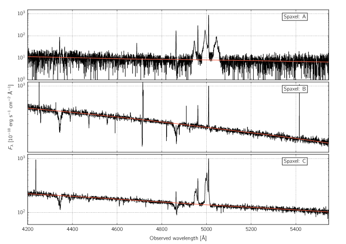
We rely on the locally weighted scatterplot smoothing (LOWESS) approach to fit the continuum for all spaxels in the blue mosaic (each spaxel being fitted individually). The LOWESS algorithm (Cleveland, 1979) is a non-parametric fitting technique that (through an iterative process) is only very weakly affected by bad pixels and/or strong emission & absorption lines in a spectra. In practice, we use the statsmodel (Seabold & Perktold, 2010) implementation of the LOWESS algorithm inside a custom-build python script. The resulting LOWESS fits are shown with red lines in Fig. 2. We stress that while the LOWESS fits do not remove stellar absorption features, the presence of these features in the continuum-subtracted datacube is of no importance for our subsequent analysis as they do not land within the [O III] spectral range.

2.2. Deblending the [O III]$\lambda\lambda$4959,5007 lines

Line-of-sight velocities $v_{los}$ for the O-rich ejecta in YSNR 1E 0102 range from:

$$-3500\text{\,km\,s${}^{-1}$}<v_{los}<+5000\text{\,km\,s${}^{-1}$}.$$ (2)

This implies Doppler shifts larger than 48 Å, the spectral gap between the [O III]$\lambda$4959 and [O III]$\lambda$5007 lines. As numerous sight-lines contain both blue- and redshifted material, the resulting total [O III]$\lambda\lambda$4959,5007 line profile is often complex (as illustrated in Fig. 2). As the intensity of the [O III]$\lambda$4959 and [O III]$\lambda$5007 forbidden emission lines are tied by a scaling factor of 2.98, their respective contributions to a given spectrum can nonetheless be disentangled through the following iterative process.

Let us define $F(\lambda)$ the continuum-subtracted flux density of a given sight-line as a function of the wavelength $\lambda$. Ignoring the presence of emission lines other than the [O III] lines, $F({\lambda})$ can be expressed as:

$$F(\lambda)=G\left(c\left(\frac{\lambda}{\lambda_{5007}}-1\right)\right)+\frac{1}{2.98}G\left(c\left(\frac{\lambda}{\lambda_{4959}}-1\right)\right)$$ (3)

with $c$ the speed of light, and $\lambda_{5007}$ & $\lambda_{4959}$ the rest wavelengths of the [O III]$\lambda$5007 & [O III]$\lambda$4959 lines. $G(v_{los})$ represents the [O III]$\lambda$5007 flux density as a function of the ejecta velocity $v_{los}$: effectively, the disentangled [O III] spectra. Re-arranging Eq. 3, $G(v_{los})$ can be expressed as:

$$G\left(v_{los}\right) = G\left(c\left(\frac{\lambda}{\lambda_{5007}}-1\right)\right)$$ (4)

$$= \sum_{i=0}^{\infty}\left\{\left(\frac{-1}{2.98}\right)^{i}F\left(\lambda\left(\frac{\lambda_{5007}}{\lambda_{4959}}\right)^{i}\right)\right\}$$

In words, disentangling the contributions from the [O III]$\lambda$4959 and [O III]$\lambda$5007 lines from a given spectrum requires to add shifted & scaled copies of the spectrum to the original one. Through this iterative process, the contamination from the [O III]$\lambda$4959 line is shifted towards shorter wavelengths by a factor of $\lambda_{5007}/\lambda_{4959}$ and scaled by $2.98^{-1}$ at each step. This process is illustrated in Fig. 3 for the first four steps of the summation in Eq. 4 for a representative WiFeS spectrum containing both red- and blueshifted ejecta. Given the range of radial velocities of the O-rich ejecta in YSNR 1E 0102, only two cleaning steps ($i_{max}=2$) are required to disentangle the [O III]$\lambda$4959 and [O III]$\lambda$5007 lines for YSNR 1E 0102.

Figure 3.— Demonstration of the iterative deblending procedure of the [O III]$\lambda\lambda$4959,5007 emission lines (for the first four steps). The black curves show the spectra of spaxel D (see Fig. 1) at cleaning step 0 to 4 (top to bottom). In each case, the red curve is the subsequent correction to be subtracted. Vertical dashed lines show the spectral range of the ejecta associated with the [O III]$\lambda$5007 line, spanning 8500 km s^-1 from $\Delta v=-3500$ km s^-1 to $\Delta v=+5000$ km s^-1. The grey-colored range shows the spectral locations of the contamination associated with the [O III]$\lambda$4959 line. Only 2 cleaning steps are required for the [O III]$\lambda$5007 spectral features to be deblended from the [O III]$\lambda$4959 component.

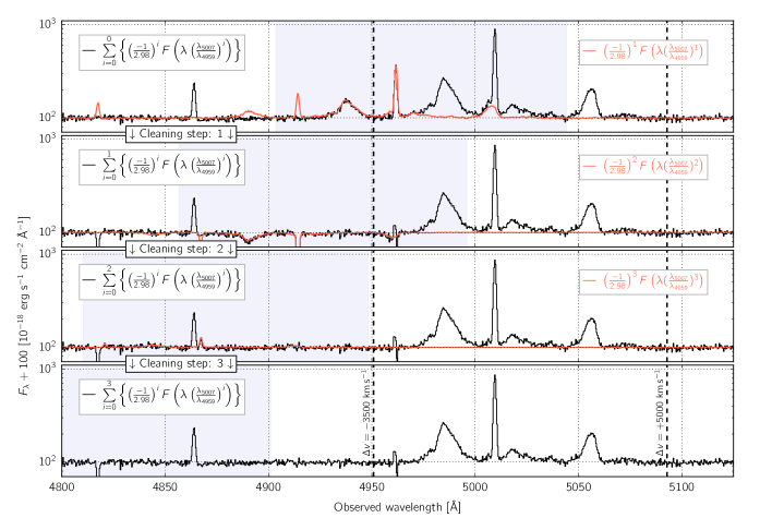
The presence of emission lines other than [O III] (e.g. H$\beta$) – and for some spaxels of stellar absorption features – leads to the creation of artefacts in the cleaned spectra: the clearest example is found at $\sim$4820 Å, and is caused by H$\beta$ during the first cleaning step. As these artefacts also move towards shorter wavelengths with each cleaning step, the lack of features red-wards of [O III]$\lambda$5007 ensures that the final disentangled [O III] line profile is clean.

Vogt & Dopita (2010) followed a similar disentangling procedure, but only performed one cleaning iteration. This was not strictly speaking sufficient to remove all contaminations from the [O III]$\lambda$4959 line (as illustrated in the second panel of Fig. 3) for all sight-lines. However, the remaining (negative) contamination where sparse and did not affect their analysis & conclusions.

3. Constructing the 3-D map of the O-rich ejecta

Having fully removed the contamination from the [O III]$\lambda$4959 line from each spectra, the WiFeS datacube can be directly converted in a 3-D map with units of [pc$\times$pc$\times$pc] via Eq. 1, assuming a distance to the SMC of 62 kpc (Graczyk et al., 2014; Scowcroft et al., 2016) and an age of 2050 yr for YSNR 1E 0102 (Finkelstein et al., 2006). We rely on the mayavi module in python (Ramachandran & Varoquaux, 2011) to create an interactive diagram of the O-rich ejecta, and export it to the x3d file format. This forms the first step of the x3d pathway, as described by Vogt et al. (2016). We refer the reader interested in using mayavi to implement the x3d pathway to the demonstration scripts published by Vogt et al. (2016) and hosted on a dedicated Github repository.

We do not here describe our python script at any length, beside the fact that we rely on the mlab.contour3d routine inside mayavi for drawing the 3-D isocontours of the [O III]$\lambda$5007 line flux density. This approach does not involve any fitting of the [O III]$\lambda$5007 line profile: we directly convert the spectral extent of the emission line profile into a spatial extent. This is motivated by the fact that the internal velocity dispersion of individual clumps $\sigma_{v}\lesssim 100$ km s^-1 is smaller than the observed width of the spectral structures of the [O III]$\lambda$5007 emission line profiles (typically $\gtrsim 500$ km s^-1), i.e. WiFeS resolves real velocity stretches (and thus spatial stretches along the line-of-sight) of spatially unresolved clumps of ejecta.

We use mlab.quiver3d for drawing additional elements in the model that include directional arrows, large wireframe spheres of 6 pc and 12 pc in radius (intended as scale reference for the model), and a black sphere of 1 pc in diameter marking the center of the model. We note that both mlab.contour3d and mlab.quiver3d are well handled by the x3d-exporter of mayavi, the current specific limitations of which were discussed in details in the online examples provided by Vogt et al. (2016).

The center of the model is defined (for the X$\equiv$East-West and Y$\equiv$North-South directions) as the ejecta’s origin derived from their proper motions (Finkelstein et al., 2006). The model reference along the Z$\equiv$line-of-sight direction is set at the SMC rest-frame, derived by fitting a Gaussian profile to the H$\beta$ line profile integrated across the entire WiFeS mosaic.

Projections of the 3-D map (as seen from the Earth, North and West) are presented in Fig. 4. There certainly exists a plethora of tools and techniques to create two-dimensional (2-D) projections of 3-D structures. For demonstration purposes, the illustrations in Fig. 4 were created using the screenshot capabilities of the online, interactive version of the model. Until the publication of the article, the online model can be accessed at http://fpavogt.github.io/x3d-pathway/YSNR.html.

Figure 4.— Reconstructed 3-D map of the [O III]$\lambda$5007 emission in 1E 0102 at the level of $3.5\times 10^{-17}$ erg s^-1 cm^-2 Å^-1, as seen from the Earth (top, to be compared with Fig. 1), the West (middle) and the North (bottom). The central black sphere is 1 pc in diameter, and marks the location of the supernova explosion derived from the ejecta proper motion (for the X-Y location), and set in the SMC rest-frame (for the Z direction). The larger wireframe sphere is 6 pc in diameter, and included in the model as a scale reference. Most [O III]-bright ejecta are located outside of this 6 pc sphere. In all panels, the red arrow points towards the Earth, the green arrow points North and the blue arrow points East. For demonstration purposes, these screenshots were generated using the Screenshot tool on the html page hosting the interactive model. Note on the arXiv version: until the publication of the article, the online model can be accessed at http://fpavogt.github.io/x3d-pathway/YSNR.html.

Creating an online interactive html page (exploiting the x3dom framework) constitutes the second phase of the x3d pathway introduced by Vogt et al. (2016). With this approach, the 3-D map of the O-rich ejecta in YSNR 1E 0102 shown in Fig. 4 is made available as an interactive model to the readers of this article via most mainstream web browsers (and without the need for specific plugins). In its most straightforward implementation, creating an interactive html document only requires some basic html code to load the x3d file (created via mayavi in this case). The x3dom environment however offer several tools that can be easily exploited with additional javascript functions. We explore some of these additional capabilities particularly suited for scientific applications in the next section.

4. Specific x3dom tools to boost the scientific value of interactive 3-D models

Vogt et al. (2016) already suggested that action buttons allowing the reader to interact with a given 3-D model can significantly enhance the scientific value of an interactive figure. The use of pre-defined viewpoints that can be toggled by the reader allow (for example) to precisely guide their attention to elements of interest, without restricting their ability to explore the model as they please. Action buttons altering the visibility of different elements inside the model can also allow readers to remove the outer layers of complex structures to reveal their inner workings.

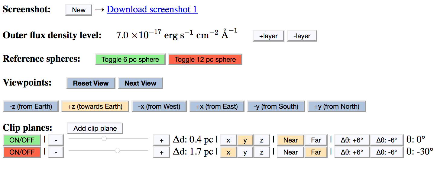
For the interactive 3-D model of YSNR 1E 0102, we have implemented additional interaction buttons, with the intention to increase the scientific usefulness of the interactive figure. In addition to the Viewpoints and Toggle buttons already used by Vogt et al. (2016), we introduce:

1. a Screenshot ability, which allows readers to easily save a png image of the interactive window in its current state,

2. the display (and live update) of the flux density level corresponding to the outer layer of the [O III]$\lambda$5007 emission visible at any given time, and

3. clip planes, which allow slicing of the model in any direction and at any angle. In particular, the offset of the clip plane from the model center (in pc) and their angle of rotation (in degrees, set by the reader) are also updated live.

The full html and javascript files used to create the online interactive model for YSNR 1E 0102 have been uploaded onto a new sub-directory within the dedicated Github repository of the x3d pathway created by Vogt et al. (2016). These files are heavily commented and once again intended as stepping stone for members of the community interested in exploiting the capabilities of the x3d pathway.

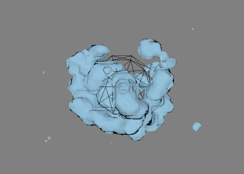
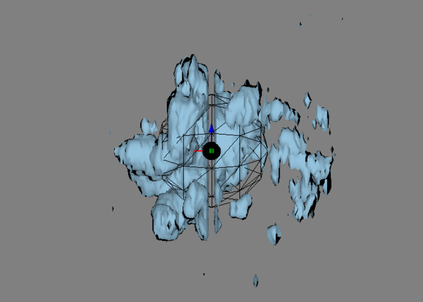
The javascript code responsible for the handling of clip planes in our interactive model of YSNR 1E 0102 has been built upon the demonstration example advertised on the official x3dom website on 2014, July 10. In comparison with the original javascript functions created by “Timo” on 2014, June 16, our version of the code contains new features, including the ability to fetch a clip plane location (its translation and rotation angle), the possibility for the user to slide a clip plane one-step-at-a-time using dedicated buttons, and the option to set a given clip-plane fully invisible (or not). Most importantly, our version of the code corrects a bug in the original version, in which the handling of a simultaneous translation and rotation led to an erroneous behavior of the outer rectangular frame associated with a given clip plane. A screenshot of the interactive model of YSNR 1E 0102 demonstrating the use of a clip plane is presented in Fig. 5. The corresponding state of the action buttons is shown in Fig. 6, for completeness. We note that beside the color-changing behavior of the action buttons, our html & javascript codes include very little styling (css-like) elements on purpose, to keep them as simple, clear and concise as possible.

Figure 5.— Screenshot of the interactive 3-D map of the oxygen-rich ejecta in YSNR 1E0102, demonstrating some of the associated x3dom visualization & analysis tools. These include the ability to peel intensity layers (the dark blue layer corresponds to a flux density level of $7\times 10^{-17}$ erg s^-1 cm^-2 Å^-1), and clip planes to slice the model at a certain location and angle. The corresponding state of the interaction buttons is shown in Fig. 6. An interactive version of this Figure is accessible in the online version of this article. Note on the arXiv version: until the publication of the article, the online model can be accessed at http://fpavogt.github.io/x3d-pathway/YSNR.html.

Figure 6.— Screenshot of the interaction buttons present on the demonstration html page hosting the 3-D map of the O-rich ejecta of YSNR 1E 0102. These buttons complement the (basic) x3dom ability to manually slide, zoom-in, zoom-out and rotate around the model; they allow to save screenshots, peel the intensity layers of the model, toggle size-reference spheres on & off, move to pre-defined viewpoints & reset the current one, as well as add clip planes to slice the model. Clip planes can be moved in full 3-D space, with their distance from the model center $\Delta$d and rotation angle $\theta$ updated automatically. The value of the flux density level of the faintest layer visible is also updated automatically.

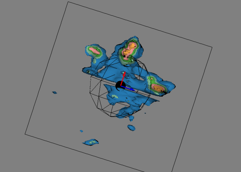
The use of clip plane(s) significantly expands the scientific potential of a given interactive 3-D model. Beyond their primary purpose of slicing through the data, they also allow the user to measure distances and angles in 3-D (provided these characteristics are communicated to the user): an important feature that effectively provides to an interactive 3-D diagram a similar level of exploitability than that of a more usual 2-D diagram (from which the value of data points can be interpolated). Clip planes are one out of many features accessible through the x3dom framework, but most certainly one of special importance for any scientific applications. We note that the interactivity offered by clip planes (and the x3dom framework in general) represents one clear step towards the suggestions of Goodman (2012) that described the importance of interactivity of 3-D diagrams (coupled with the ability to link different views and diagrams with one another).

5. Summary

In this article, we have demonstrated the potential of the x3d pathway for optical IFS observations with YSNR 1E 0102 in the SMC as an example. Using the 3-D map of the oxygen-rich ejecta in this system, we have exploited the x3d pathway introduced by Vogt et al. (2016) to create an interactive 3-D model of YSNR 1E 0102 hosted in an html document, accessible via most mainstream web browsers. We have explored additional features of the x3dom framework to increase the scientific potential of interactive 3-D diagrams, in particular the possibility of using clip planes to slice through the data. Our corrected and enhanced set of javascript functions designed to handle clip planes (originally shared on the x3dom website), and allowing users to extract scientifically valid information from a given 3-D model – i.e. distances and angles – is made freely available to the scientific community on a dedicated Github repository.

At the time of publication of this article, the x3d pathway is already actively supported by leading journals in the field of astrophysics. The generation of 3-D models (and their export to the x3d format) thus most certainly remains the biggest hurdle in terms of implementation and a clear obstacle slowing the expansion of the x3d pathway in the field of astrophysics. The mayavi module in python offers a simple, pythonic tool for astronomers to create 3-D models, although specific limitations still impede on the creation of more advanced products (Punzo et al., 2015; Vogt et al., 2016). blender is an open-source alternative to mayavi that offers a nearly unlimited set of options and tools, but at the price of an extremely steep learning curve. From that perspective, recent efforts like frelled (Taylor, 2015) and astroblend (Naiman, 2016) aiming at bringing blender closer to astronomers are certainly worth mentioning (see also Kent, 2013, 2015).

The x3dom framework is oblivious to the manner a given 3-D model is generated. It is therefore of no importance (from the perspective of the x3d pathway) whether the mayavi limitations will be gradually addressed or not, whether tools such as astroblend and frelled will become increasingly popular within our community, or whether other dedicated software solutions will keep emerging (see e.g. Barnes et al., 2006; Steffen et al., 2011; Woodring et al., 2011; Punzo et al., 2016): that is, so long as our tools support model exports to the x3d format.

Most importantly, the future of the x3dom framework, intended to be the way that 3-D models are shared on the World Wide Web, is tied to much more than its sole use within the field of astrophysics. From that perspective, we believe that our choice as a community does not lie in deciding on the likelihood of a future for this technology, but rather in how soon we shall actively embrace the potential of the x3d pathway to improve our ability to share & publish complex multi-dimensional datasets. We note that the creation of a dedicated astrophysics working group within the Web3D Consortium would give our community the ability to exert a direct influence on the evolution of the x3dom framework, in a similar fashion to that already pursued by the medical working group towards a better support of human anatomy representation.

References

- Astropy Collaboration et al. (2013) Astropy Collaboration, Robitaille, T. P., Tollerud, E. J., Greenfield, P., Droettboom, M., Bray, E., Aldcroft, T., Davis, M., Ginsburg, A., Price-Whelan, A. M., Kerzendorf, W. E., Conley, A., Crighton, N., Barbary, K., Muna, D., Ferguson, H., Grollier, F., Parikh, M. M., Nair, P. H., Unther, H. M., Deil, C., Woillez, J., Conseil, S., Kramer, R., Turner, J. E. H., Singer, L., Fox, R., Weaver, B. A., Zabalza, V., Edwards, Z. I., Azalee Bostroem, K., Burke, D. J., Casey, A. R., Crawford, S. M., Dencheva, N., Ely, J., Jenness, T., Labrie, K., Lim, P. L., Pierfederici, F., Pontzen, A., Ptak, A., Refsdal, B., Servillat, M., & Streicher, O. 2013, A&A, 558, A33
- Barnes et al. (2006) Barnes, D. G., Fluke, C. J., Bourke, P. D., & Parry, O. T. 2006, Publications of the Astronomical Society of Australia, 23, 82
- Bonnarel et al. (2000) Bonnarel, F., Fernique, P., Bienaymé, O., Egret, D., Genova, F., Louys, M., Ochsenbein, F., Wenger, M., & Bartlett, J. G. 2000, A&ASupplement Series, 143, 33
- Chevalier & Kirshner (1979) Chevalier, R. A. & Kirshner, R. P. 1979, ApJ, 233, 154
- Childress et al. (2014a) Childress, M., Vogt, F., Nielsen, J., & Sharp, R. 2014a, Astrophysics Source Code Library, ascl:1402.034
- Childress et al. (2014b) Childress, M. J., Vogt, F. P. A., Nielsen, J., & Sharp, R. G. 2014b, Ap&SS, 349, 617
- Cleveland (1979) Cleveland, W. S. 1979, Journal of the American Statistical Association, 74, 829
- Danziger & Dennefeld (1976a) Danziger, I. J. & Dennefeld, M. 1976a, PASP, 88, 44
- Danziger & Dennefeld (1976b) —. 1976b, ApJ, 207, 394
- Dopita et al. (2007) Dopita, M., Hart, J., McGregor, P., Oates, P., Bloxham, G., & Jones, D. 2007, Ap&SS, 310, 255
- Dopita et al. (2010) Dopita, M., Rhee, J., Farage, C., McGregor, P., Bloxham, G., Green, A., Roberts, B., Neilson, J., Wilson, G., Young, P., Firth, P., Busarello, G., & Merluzzi, P. 2010, Ap&SS, 327, 245
- Dopita et al. (1981) Dopita, M. A., Tuohy, I. R., & Mathewson, D. S. 1981, The ApJ, 248, L105
- Fesen et al. (2006) Fesen, R. A., Hammell, M. C., Morse, J., Chevalier, R. A., Borkowski, K. J., Dopita, M. A., Gerardy, C. L., Lawrence, S. S., Raymond, J. C., & van den Bergh, S. 2006, ApJ, 645, 283
- Finkelstein et al. (2006) Finkelstein, S. L., Morse, J. A., Green, J. C., Linsky, J. L., Shull, J. M., Snow, T. P., Stocke, J. T., Brownsberger, K. R., Ebbets, D. C., Wilkinson, E., Heap, S. R., Leitherer, C., Savage, B. D., Siegmund, O. H., & Stern, A. 2006, ApJ, 641, 919
- Goodman (2012) Goodman, A. A. 2012, Astron. Nachr., 333, 505
- Goss et al. (1979) Goss, W. M., Shaver, P. A., Zealey, W. J., Murdin, P., & Clark, D. H. 1979, MNRAS, 188, 357
- Graczyk et al. (2014) Graczyk, D., Pietrzyński, G., Thompson, I. B., Gieren, W., Pilecki, B., Konorski, P., Udalski, A., Soszyński, I., Villanova, S., Górski, M., Suchomska, K., Karczmarek, P., Kudritzki, R.-P., Bresolin, F., & Gallenne, A. 2014, ApJ, 780, 59
- Hendrick et al. (2005) Hendrick, S. P., Reynolds, S. P., & Borkowski, K. J. 2005, The ApJ, 622, L117
- Hunter (2007) Hunter, J. D. 2007, Computing in Science and Engineering, 9, 90
- Joye & Mandel (2003) Joye, W. A. & Mandel, E. 2003, in , 489
- Kent (2013) Kent, B. R. 2013, PASP, 125, 731
- Kent (2015) —. 2015, 3D Scientific Visualization with Blender
- Lasker (1978) Lasker, B. M. 1978, ApJ, 223, 109
- Mathewson et al. (1980) Mathewson, D. S., Dopita, M. A., Tuohy, I. R., & Ford, V. L. 1980, The ApJ, 242, L73
- Mathewson et al. (2013) Mathewson, D. S., Hart, J., Wehner, H. P., Hovey, G. R., & van Harmelen, J. 2013, Journal of Astronomical History and Heritage, 16, 2
- Milisavljevic & Fesen (2013) Milisavljevic, D. & Fesen, R. A. 2013, ApJ, 772, 134
- Murdin & Clark (1979) Murdin, P. & Clark, D. H. 1979, MNRAS, 189, 501
- Naiman (2016) Naiman, J. P. 2016, Astronomy and Computing, 15, 50
- Park et al. (2003) Park, S., Hughes, J. P., Burrows, D. N., Slane, P. O., Nousek, J. A., & Garmire, G. P. 2003, The ApJ, 598, L95
- Punzo et al. (2016) Punzo, D., van der Hulst, J. M., & Roerdink, J. B. T. M. 2016, ArXiv e-prints, 1609, arXiv:1609.03782
- Punzo et al. (2015) Punzo, D., van der Hulst, J. M., Roerdink, J. B. T. M., Oosterloo, T. A., Ramatsoku, M., & Verheijen, M. A. W. 2015, Astronomy and Computing, 12, 86
- Ramachandran & Varoquaux (2011) Ramachandran, P. & Varoquaux, G. 2011, IEEE Computing in Science & Engineering, 13, 40
- Schenck et al. (2014) Schenck, A., Park, S., Burrows, D. N., Hughes, J. P., Lee, J.-J., & Mori, K. 2014, ApJ, 791, 50
- Scowcroft et al. (2016) Scowcroft, V., Freedman, W. L., Madore, B. F., Monson, A., Persson, S. E., Rich, J., Seibert, M., & Rigby, J. R. 2016, ApJ, 816, 49
- Seabold & Perktold (2010) Seabold, S. & Perktold, J. 2010, in Proc. of the 9th Python in Science Conference, 57–61
- Steffen et al. (2011) Steffen, W., Koning, N., Wenger, S., Morisset, C., & Magnor, M. 2011, IEEE Transactions on Visualization and Computer Graphics, Volume 17, Issue 4, p.454-465, 17, 454
- Sutherland & Dopita (1995) Sutherland, R. S. & Dopita, M. A. 1995, ApJ, 439, 381
- Taylor (2015) Taylor, R. 2015, Astronomy and Computing, 13, 67
- Thorstensen et al. (2001) Thorstensen, J. R., Fesen, R. A., & van den Bergh, S. 2001, AJ, 122, 297
- Tuohy & Dopita (1983) Tuohy, I. R. & Dopita, M. A. 1983, The ApJ, 268, L11
- van den Bergh & Dodd (1970) van den Bergh, S. & Dodd, W. W. 1970, ApJ, 162, 485
- Vogt & Dopita (2010) Vogt, F. & Dopita, M. A. 2010, ApJ, 721, 597
- Vogt & Dopita (2011) —. 2011, Ap&SS, 331, 521
- Vogt et al. (2014) Vogt, F. P. A., Dopita, M. A., Kewley, L. J., Sutherland, R. S., Scharwächter, J., Basurah, H. M., Ali, A., & Amer, M. A. 2014, ApJ, 793, 127
- Vogt et al. (2016) Vogt, F. P. A., Owen, C. I., Verdes-Montenegro, L., & Borthakur, S. 2016, ApJ, 818, 115
- Winkler & Kirshner (1985) Winkler, P. F. & Kirshner, R. P. 1985, ApJ, 299, 981
- Winkler et al. (2009) Winkler, P. F., Twelker, K., Reith, C. N., & Long, K. S. 2009, ApJ, 692, 1489
- Woodring et al. (2011) Woodring, J., Heitmann, K., Ahrens, J., Fasel, P., Hsu, C.-H., Habib, S., & Pope, A. 2011, ApJS, 195, 11