Quantum cosmology in an anisotropic n-dimensional universe

Abstract

We investigate quantum cosmological models in an n-dimensional anisotropic universe in the presence of a massless scalar field. Our basic inspiration comes from Chodos and Detweiler’s classical model which predicts an interesting behaviour of the extra dimension, shrinking down as time goes by. We work in the framework of a  recent geometrical scalar-tensor theory of gravity. Classically, we obtain two distinct type of solutions. One of them has an initial singularity while the other represents a static universe considered as a whole. By using the canonical approach to quantum cosmology, we investigate how quantum effects could have had an influence in the past history of these universes.

1 Introduction

In the last decades a great deal of work has gone into scalar-tensor theories of gravity, particularly in the context of inflationary models and also in attempts to explain the observed acceleration of the universe. In all these, the scalar field plays an essential role, although its nature and origin as yet remains unclear. However, in a recently proposed scalar-tensor theory, the nature of the scalar field is attributed to the space-time geometry [1]. In this picture, physical and geometrical objects are, by construction, invariant under a new group of symmetry, namely, the group of Weyl transformations, and this leads to a natural mapping between the action of a scalar-tensor theory with a non-minimally coupled scalar field in a non-Riemannian space-time and the action of general relativity with a massless scalar field coupled to gravity through a dimensionless parameter. Recent applications of this new theoretical proposal to cosmology include scenarios displaying unusual geometrical space-time behaviour [2].

Among other alternative approaches to gravity theories, in which the scalar field emerges, we would like to call attention for the modern $n$-dimensional models of the universe. These have been developed in many different contexts, starting from the seminal Kaluza-Klein ideas to string cosmology [3]. Even in a purely classical general relativistic framework a particular appealing cosmological model worth of mentioning is the one obtained in general relativity by Chodos and Detweiler, who put forward the idea that the present stage of the Universe evolved from a five-dimensional scenario in which the extra dimension becomes unobservably small due to a kind of dynamical contraction [4]. Following the same direction,  other higher-dimensional general anisotropic models have been considered also in scalar-tensor theories of gravity [5].

The introduction of scalar fields and higher dimensions are also motivated by the attempt to answer many open questions in classical cosmology, particularly those related to the early phases of the universe. One possibility of examining these questions in a deeper way is to go beyond the classical level and look for a new picture in which quantum effects are taken into account. An important contribution to this line of research has been provided by the quantum cosmology program [6]. It should be said, however, that there are currently many technical and conceptual difficulties with this approach. For instance, a well known problem in quantum cosmology is the definition of time, a problem often referred to as the problem of time [7]. Indeed, it turns out that quantum cosmology does not specify in a unique way a parameter that plays the role of time. In the general relativistic context, there have been several attempts to overcome this difficulty. A well known way of tackling the problem is by introducing matter content into the model, the latter usually being represented by a scalar field associated to a fluid with a barotropic equation of state [8]. Another interesting attempt to find a possible solution to the problem of time in the framework of Brans-Dicke theory was given recently [9], in which there is no need to add matter in the form of a scalar field as the gravitational theory itself provides such a field . By choosing suitable canonical transformations, the Brans-Dicke scalar field may be identified with time in the sense of the usual Schrödinger picture. By the same token, in the quantization of a geometrical scalar-tensor theory we can naturally relate the intrinsic scalar field to a parameter that measures the evolution of the system at the quantum level.

The goal of the present work is to analyse quantum cosmological scenarios predicted by the geometrical scalar-tensor theory in an anisotropic n-dimensional space-time. In the context of general relativity, a similar problem was recently considered by P. Letelier [11]. The paper is organized as follows. We begin, in Section 2, with a brief review of the basic tenets of the geometrical scalar-tensor gravitational theory. In Section 3, we present the classical solutions of the n-dimensional model in the light of the Lagrangian formalism. We then proceed to perform the Hamiltonian formalism and propose some canonical transformations to decouple the canonical variables. We check that the solutions obtained from the Lagrangian formalism are also solutions of the Hamiltonian equations. Next, in Section 4, we carry out the canonical quantization of the model. By assuming that the classical geometry has a flat spatial section we obtain the wave function of the universe and calculate the expectation values according to the many-worlds interpretation. Finally, in Section 6, we discuss our results.

2 The geometrical gravitational theory

Let us begin by considering the gravitational sector of the non-minimally coupled scalar-tensor action

$$\mathcal{S}=\int d^{n}x\sqrt{|g|}\left[e^{-\phi}\left(R+\omega g^{\mu\nu}\phi_{,\mu}\phi_{,\nu}\right)-V(\phi)\right],$$ (1)

defined on a $n$-dimensional space-time , with $R$ denoting the $n$-dimensional curvature scalar , $g$ the determinant of the metric tensor $g_{\mu\nu}$, and $\omega$ being a dimensionless parameter. As in the four-dimensional case, the field equations for $g_{\mu\nu}$ and $\phi$, together with the non-metricity condition that characterizes a Weyl integrable space-time (WIST), are easily obtained by applying the Palatini’s variational method to the above action (See ref. [1]). Thus, the variation of (1) with respect to the affine connection leads to

$$\nabla_{\alpha}g^{\mu\nu}=-\frac{2}{n-2}\phi_{,\alpha}\;g^{\mu\nu},$$ (2)

where $\phi_{,\alpha}=\partial_{\alpha}\phi$. This is precisely the non-metricity condition mentioned above, and that, in a certain sense, leads, from first principles, to the determination of the space-time geometry [13] . From the above $\psi=\frac{2}{n-2}\phi$ plays the role of the n-dimensional Weyl scalar field . In the terminology of the geometrical scalar-tensor theory, a Weyl frame is the set $(M,g,\psi)$ characterized by the metric tensor $g$ and the scalar field $\psi$ defined on the manifold $M$. An important property of the Weyl geometry is that the non-metricity condition $\nabla_{\alpha}g^{\mu\nu}=-\psi_{,\alpha}g^{\mu\nu}$ is invariant under the set of transformations

$$\bar{g}_{\mu\nu} =e^{f}g_{\mu\nu},$$ (3)

$$\bar{\psi} =\psi+f.$$

That is, in the new frame $(M,\bar{g},\bar{\psi})$ we have $\nabla_{\alpha}\overline{g}^{\mu\nu}=-\bar{\psi}_{,\alpha}\overline{g}^{\mu\nu}$. Clearly, these transformations preserve the geodesic curves, since the affine connection is kept invariant. Because $\bar{g}_{\mu\nu}$ and $g_{\mu\nu}$ are related by a conformal transformation the causal structure these metric define on the manifold $M$ does not change when we go from one Weyl frame to another. By setting $f=-\frac{2}{n-2}\phi=-\psi$ in (3) we have $\bar{\psi}=0$. Because we recover the Riemannian compatibility condition between the metric and affine connection, this frame is usually called the Riemann frame, and is denoted as the set $(M,\bar{g},0)$.

It is not difficult to verify that in the Riemann frame $(M,\bar{g},0)$ the action (1) becomes

$$\mathcal{\bar{S}}=\int d^{n}x\sqrt{|\bar{g}|}\left[\bar{R}+\omega\bar{g}^{\mu\nu}\phi_{,\mu}\phi_{,\nu}-e^{\frac{n}{n-2}\phi}V(\phi)\right],$$ (4)

which, for $\omega=\frac{1}{2}$, is formally identical to the $n$-dimensional Hilbert-Einstein action of a scalar field minimally coupled with gravity with a potential $U(\phi)$ given by $U(\phi)=e^{\frac{n}{n-2}\phi}V(\phi)$. In fact, the analogy between the two configurations is even more apparent if we recall that in the Riemann frame, particles and light rays will follow Riemannian metric and affine geodesics, respectively. In the next section, we shall investigate the cosmological scenarios that are generated by the action (4), when we take $V(\phi)=0$.

3 The Classical Cosmological Model

3.1 The Lagrangian formalism

We shall now consider the n-dimensional, $n>4$, anisotropic cosmological model whose geometry is described by the following line element

$$ds^{2}=N(t)^{2}dt^{2}-a(t)^{2}\left(dx^{2}+dy^{2}+dz^{2}\right)-b(t)^{2}\sum_{i=1}^{n-4}{dl_{i}}^{2},$$ (5)

with $N(t)$ denoting the lapse function, $a(t)$ being the scale factor associated with the usual three spatial dimensions, and $b(t)$ representing the scale factor of the $(n-4)$-dimensions, the latter being assumed to be compact.

The reduced action corresponding to (4) written in terms of the geometry given by the line element (5) takes the following form:

$$\mathcal{S}_{\text{red}}=V_{o}\int dt\left[-\frac{6}{N}\dot{a}^{2}ab^{n-4}-\frac{6(n-4)}{N}\dot{b}\dot{a}a^{2}b^{n-5}-\frac{(n-4)(n-5)}{N}\dot{b}^{2}a^{3}b^{n-6}+\frac{\omega}{N}a^{3}b^{n-4}\dot{\phi}^{2}\right],$$ (6)

where the over dot denotes differentiation with respect to the time coordinate $t$, while $V_{o}$ stands for the integration on the $(n-1)$-dimensional space defined by the compact extra dimensions . From (6) we write the Lagrangian of the model as

$$L\equiv-\frac{6}{N}\dot{a}^{2}ab^{n-4}-\frac{6(n-4)}{N}\dot{b}\dot{a}a^{2}b^{n-5}-\frac{(n-4)(n-5)}{N}\dot{b}^{2}a^{3}b^{n-6}+\frac{\omega}{N}a^{3}b^{n-4}\dot{\phi}^{2}.$$ (7)

Now, if we set $N(t)\equiv 1$, the field equations, obtained from the Euler-Lagrange equations, are

$$3H_{a}^{2}+3(n-4)H_{a}H_{b}+\frac{(n-4)(n-5)}{2}H_{b}^{2} =\frac{\omega}{2}\dot{\phi}^{2},$$

$$2\dot{H}_{a}+3H_{a}^{2}+(n-4)\dot{H}_{b}+2(n-4)H_{a}H_{b}+\frac{(n-3)(n-4)}{2}H_{b}^{2} =-\frac{\omega}{2}\dot{\phi}^{2},$$ (8)

$$3\dot{H}_{a}+6H_{a}^{2}+(n-5)\dot{H}_{b}+3(n-5)H_{a}H_{b}+\frac{(n-4)(n-5)}{2}H_{b}^{2} =-\frac{\omega}{2}\dot{\phi}^{2},$$

$$3H_{a}\dot{\phi}+(n-4)H_{b}\dot{\phi}+\ddot{\phi} =0,$$

where we are defining $H_{a}=\frac{\dot{a}}{a}$ and $H_{b}=\frac{\dot{b}}{b}$. A solution of the equations of motion above is given by the following set

$$a(t)=a_{0}|C(t-t_{0})-1|^{\frac{1}{6}},\qquad b(t)=b_{0}|C(t-t_{0})-1|^{\frac{1}{2(n-4)}},\qquad\phi(t)=\phi_{0}\pm\sqrt{\frac{1}{\omega}\left(\frac{2}{3}+\frac{n-5}{4(n-4)}\right)}\;\ln|C(t-t_{0})-1|,$$ (9)

with $a_{0}$, $b_{0}$, $\phi_{0}$ and $C$ denoting integration constants. It is not difficult to verify that the solutions (9) represent a universe in which both the usual three dimensions and the extra $n-4$ dimensions expands as time passes, with a space-time singularity at $t=t_{0}+1/C$ (See, Fig. 1 below) 1. In this solution, since the scalar field is a real function of time, it is required that $\omega>0$.

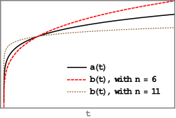
Figure 1: Scale factors in (9)

On the other hand, a set of distinct solutions is given by

$$a(t)=a_{0}|C(t-t_{0})-1|^{\frac{(10-n)}{18}},\qquad b(t)=b_{0}|C(t-t_{0})-1|^{\frac{1}{6}},\qquad\phi(t)=\phi_{0}\pm\frac{1}{6}\sqrt{\frac{-n^{2}+17n+20}{3\omega}}\;\ln|C(t-t_{0})-1|.$$ (10)

As in the previous solution (9), the behaviour of the scale factor of the extra dimensions (10) leads to a singularity as $t\rightarrow t_{0}+1/C$. There are, however, some differences in this case. While the extra dimensions always expand, the behaviour of the $3$-dimensional spatial dimensions depends on the dimensionality of the model: If $n<10$, then they start from a singularity at $t=t_{0}$ and expand forever; if $n>10$, they undergo indefinitely a contraction phase; and if $n=10$, they remain constant as $a(t)=a_{0}=const$. In Figure 2, we show the behaviour of both scale factors, $a(t)$ and $b(t),$ for $n=6$ and $n=11$. Let us also note that $\omega$ must be positive for $n<19,$ and negative for $n\geq 19$.

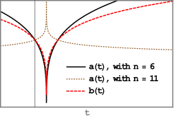
(a)

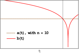
(b)

Figure 2: Scale factors in (10)

Here, it is interesting to note that according  to (10), a curious scenario arises when $n=10$. In that case, the $3$-dimensional scale factor $a$ is constant. On the other hand, if we consider the time interval between $t_{0}$ and the finite time $t_{0}+1/C$, we see that the scale factor $b(t)$ goes to zero as $t\rightarrow t_{0}+1/C$ (see Fig. 2b). This could perhaps be interpreted as a sort of pre-inflationary period when, immediately after the beginning of the universe, a dynamical compactification of the extra dimensions takes place.

If we now turn our attention to the expansion factor of the universe, a simple calculation from (5) yields

$$\Theta_{(n)}=\frac{\dot{N}}{N}+6H_{a}+2(n-4)H_{b}.$$ (11)

At this point, it should be mentioned that the expansion factor (11) calculated for the solutions (9) and (10) is given by

$$\Theta=\frac{3}{|C(t-t_{0})-1|}.$$ (12)

That is, $\Theta_{(n)}$ has the same value and does not depend on the dimension $n$. In both cases, we have expanding universes in which the expansion rate decreases with time (see Figure 3).

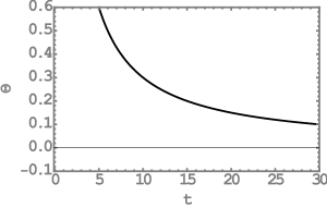
Figure 3: Expansion factor in (12)

Let us now consider two other different sets of solutions to the system of equations (3.1), which are given by

$$a(t)=a_{0}\exp\bigl{[}\Lambda_{a}(t-t_{0})\bigr{]},\qquad b(t)=b_{0}\exp\bigl{[}-\Lambda_{b}(t-t_{0})\bigr{]},\qquad\phi(t)=\phi_{0}+D(t-t_{0}),$$ (13)

and

$$a(t)=a_{0}\exp\bigl{[}-\Lambda_{a}(t-t_{0})\bigr{]},\qquad b(t)=b_{0}\exp\bigl{[}\Lambda_{b}(t-t_{0})\bigr{]},\qquad\phi(t)=\phi_{0}+D(t-t_{0}),$$ (14)

where

$$\Lambda_{a}=\sqrt{-\frac{(n-4)D^{2}\omega}{3(n-1)}}\qquad\text{and}\qquad\Lambda_{b}=\sqrt{-\frac{3D^{2}\omega}{(n-1)(n-4)}},$$ (15)

with $D$ being an integration constant, $\omega<0$, $a_{0}$, $b_{0}$, and $\phi_{0}$ as defined above. Note that the solutions (13) and (14) describe distinct scenarios. In the first, the $4$-dimensional part of the universe is expanding while, the extra- dimensional part is contracting. In the second, the dynamics of the universe is reversed: the $4$-dimensional part collapses, while the extra dimensions become larger (See Figure 4). Moreover, as it is clear from (13) and (14), in these universes there is no space-time singularity. For the expansion factor, we have, from (11)

$$\Theta_{(n)}=0,$$

which means that, according to these models, the universe, as a whole, would have no dynamics.

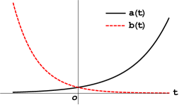
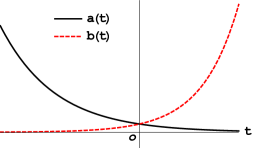
Figure 4: From left to right, scale factors in (13) and (14) respectively

3.2 The Hamiltonian formalism

As we have already mentioned, the aim of this work is to investigate quantum cosmological scenarios predicted by the geometrical scalar-tensor theory in the case of anisotropic n-dimensional space-time. Following the methods of canonical quantum cosmology, the first step is to carry out the canonical quantization of the classical model. Thus let us compute the classical Hamiltonian from the corresponding Lagrangian (7).

It is not difficult to verify that the canonical momenta corresponding to the variables $a,b$ and $\phi$ will be given, respectively, by

$$P_{a} =-\frac{12}{N}ab^{n-4}\dot{a}-\frac{6(n-4)}{N}a^{2}b^{n-5}\dot{b},$$

$$P_{b} =-\frac{2(n-4)(n-5)}{N}b^{n-6}a^{3}\dot{b}-\frac{6(n-4)}{N}b^{n-5}a^{2}\dot{a},$$ (16)

$$P_{\phi} =\frac{2\omega}{N}a^{3}b^{n-4}\dot{\phi}.$$

For $n>4$, the Hamiltonian takes the form

$$\mathcal{H}=\frac{N}{(n-2)ab^{n-6}}\left[\frac{(n-5)}{12}\frac{{P_{a}}^{2}}{b^{2}}+\frac{1}{2(n-4)}\frac{{P_{b}}^{2}}{a^{2}}-\frac{P_{a}P_{b}}{2ab}+\frac{(n-2)}{4\omega a^{2}b^{2}}{P_{\phi}}^{2}\right].$$ (17)

It turns out, however, that, the above form of $\mathcal{H}$ is not suitable for working out the canonical quantization.  A more convenient expression for $\mathcal{H}$ can be obtained if we perform the following canonical transformations: $A=\ln{a}$, $P_{A}=aP_{a}$, $B=\ln{b}$, $P_{B}=bP_{b}$, $T=\frac{\phi}{P_{\phi}}$ and $P_{T}=\frac{{p_{\phi}}^{2}}{2}$ [9, 14]. The new Hamiltonian written in terms of the new variables will be given by

$$\bar{\mathcal{H}}=\bar{N}\left[\frac{\omega(n-5)}{6(n-2)}{P_{A}}^{2}-\frac{\omega}{n-2}{P_{A}}{P_{B}}+\frac{\omega}{(n-2)(n-4)}{P_{B}}^{2}+P_{T}\right],$$ (18)

with $\bar{N}=\frac{N}{2\omega a^{3}b^{n-4}}$, which, then, leads to the equations of motion

$$\dot{A}=\frac{\bar{N}\omega}{n-2}\left(\frac{n-5}{3}P_{A}-P_{B}\right)\qquad \text{,}\qquad\dot{P}_{A}=0,$$

$$\dot{B}=\frac{\bar{N}\omega}{n-2}\left(\frac{2}{n-4}P_{B}-\frac{P_{A}}{n-2}\right)\qquad \text{,}\qquad\dot{P}_{B}=0,$$ (19)

$$\dot{T}=\bar{N}\qquad \text{and}\qquad\dot{P}_{T}=0.$$

The solution of the above system (3.2) is easily obtained, and is given by

$$a(T) =a_{0}\exp\left[\frac{\omega}{n-2}\left(\frac{n-5}{3}P_{A}-P_{B}\right)T\right],$$

$$b(T) =b_{0}\exp\left[\frac{\omega}{n-2}\left(\frac{2}{n-4}P_{B}-\frac{P_{A}}{n-2}\right)T\right],$$ (20)

$$\phi(T) =\pm\sqrt{2P_{T}}T,$$

with $P_{A}$, $P_{B}$ and $P_{T}$ being constants. As expected, one can easily verify that (9), (10), (13) and (14) are solutions of (3.2) when we set $T\propto\phi$.

4 The canonical quantization of the model

4.1 The Wheeler-DeWitt equation

In this section, we proceed with the quantization of the classical cosmological model. By following the canonical quantization prescription

$$P_{A}\rightarrow-i\frac{\partial}{\partial A}\qquad\text{,}\qquad P_{B}\rightarrow-i\frac{\partial}{\partial B}\qquad\text{,}\qquad P_{T}\rightarrow-i\frac{\partial}{\partial T},$$ (21)

the Wheeler-DeWitt equation

$$\hat{H}\Psi(A,B,T)=0,$$ (22)

takes the form

$$\left\{-\frac{\omega(n-5)}{6(n-2)}\frac{\partial^{2}}{\partial A^{2}}+\frac{\omega}{n-2}\frac{\partial^{2}}{\partial A\partial B}-\frac{\omega}{(n-2)(n-4)}\frac{\partial^{2}}{\partial B^{2}}\right\}\Psi(A,B,T)=i\frac{\partial}{\partial T}\Psi(A,B,T),$$ (23)

where $\hat{H}$ denotes the operator corresponding to $H$ (defined by $\bar{\mathcal{H}}=\bar{N}H$ according to (18)) and $\Psi$ stands for the wave function of the universe. Clearly, Eq. (22) may be identified with the Schrödinger equation $\hat{H}\Psi=i\frac{\partial\Psi}{\partial T}$, where $T$ plays the role of the parameter that measures the time evolution of the quantum system in question. Let us just recall that the Hamiltonian $\hat{H}$ is required to be a hermitian operator, with the usual inner product defined on $L^{2}$ as

$$\left\langle\Psi_{1}\vphantom{\Psi_{2}}\right|\left.\Psi_{2}\vphantom{\Psi_{1}}\right\rangle=\int_{-\infty}^{\infty}dA\int_{-\infty}^{\infty}dB\Psi_{1}^{\ast}\Psi_{2},$$

where are $\Psi_{1},\Psi_{2}$ are complex-valued measurable functions, satisfying the boundary conditions

$$\Psi(A\rightarrow\pm\infty)=0,\qquad\Psi(B\rightarrow\pm\infty)=0\qquad(Dirichlet\;\;condition),$$

or

$$\frac{\partial\Psi}{\partial A}(A\rightarrow\pm\infty)=0,\qquad\frac{\partial\Psi}{\partial A}(B\rightarrow\pm\infty)=0,\qquad\frac{\partial\Psi}{\partial B}(B\rightarrow\pm\infty)=0,\qquad\frac{\partial\Psi}{\partial B}(A\rightarrow\pm\infty)=0\qquad(Neumann\;\;condition).$$

At this point it is interesting to note that for $n=5$ the first term on the left hand side in (18) vanishes and hence the Schrödinger equation takes the simple form

$$\frac{\omega}{3}\left[\frac{\partial^{2}}{\partial B^{2}}-\frac{\partial^{2}}{\partial A\partial B}\right]\Psi(A,B,T)=-i\frac{\partial}{\partial T}\Psi(A,B,T).$$ (24)

Because of this great simplification we shall consider the case $n=5$ separately. The more general case corresponding to $n>5$ will be presented next. For the sake of completeness, the quantization of the five-dimensional model will be analyzed in Section 5.

4.2 Solutions and expectation values for an n-dimensional quantum universe

Since the Hamiltonian does not dependent on time explicitly we shall look for stationary solutions of the form

$$\Psi(A,B,T)=\Phi(A,B)e^{-iET},$$ (25)

where $E$ is a constant. As is well known, this leads to the time-independent Schrödinger equation

$$\hat{H}\Phi(A,B)=E\Phi(A,B).$$

If we now define new variables $u$ and $v$ by

$$u=\sqrt{\frac{6(n-2)}{|\omega|(n-5)}}A+\sqrt{\frac{(n-2)(n-4)}{|\omega|}}B\qquad v=\sqrt{\frac{6(n-2)}{|\omega|(n-5)}}A-\sqrt{\frac{(n-2)(n-4)}{|\omega|}}B,$$ (26)

then Eq.(23) takes the form

$$\left[\eta^{(-)}\frac{\partial^{2}}{\partial u^{2}}+\eta^{(+)}\frac{\partial^{2}}{\partial v^{2}}+E\right]\Phi(u,v)=0,$$ (27)

where we have introduced the constants

$$\eta^{(\pm)}=2\pm\sqrt{\frac{6(n-4)}{n-5}},$$

and, for simplicity, we shall take $\omega>0$. To solve Eq.(27) we write $\Phi(u,v)=\mathrm{U}(u)\mathrm{V}(v).$ This gives rise to the differential equations

$$\frac{d^{2}\mathrm{U}}{du^{2}}+\frac{\lambda}{\eta^{(-)}}\mathrm{U} =0,$$

$$\frac{d^{2}\mathrm{V}}{dv^{2}}+\frac{E-\lambda}{\eta^{(+)}}\mathrm{V} =0,$$ (28)

where $\lambda$ is a constant.

A particular solution to Eq.(27) will then easily be given by

$$\Phi_{\lambda,E}(\bar{u},\bar{v})=K\sin(\bar{u}\sqrt{\lambda})\sin(\bar{v}\sqrt{E+\lambda}),$$ (29)

where $\bar{u}=\frac{u}{\sqrt{|\eta^{(-)}|}}$ and $\bar{v}=\frac{v}{\sqrt{\eta^{(+)}}}$ , $K$ is an arbitrary constant, and we are taking $\lambda>0$ and $E>-\lambda$. Clearly, the general solution to Eq.(23) is given by superposing the functions $\Psi_{\lambda,E}(\bar{u},\bar{v},T)$, that is,

$$\Psi(\bar{u},\bar{v},T)=K\int_{0}^{\infty}dE_{1}\int_{0}^{\infty}dE_{2}F(E_{1},E_{2})e^{-i(E_{2}-E_{1})T}\sin(\bar{u}\sqrt{E_{1}})\sin(\bar{v}\sqrt{E_{2}}),$$ (30)

where we are setting $E_{1}=\lambda$, $E_{2}=E+\lambda$, and $F(E_{1},E_{2})$ is a suitable weight function chosen to construct wave packets.

We are now going to choose a particular solution from (30) by taking $F(E_{1},E_{2})=\exp\bigl{[}-\xi(E_{1}+E_{2})\bigr{]}$. It is not difficult to verify that with this choice the normalized wave function reads

$$\Psi(\bar{u},\bar{v},T)=\sqrt{\frac{\sqrt{3(n-2)(n-4)}}{\omega\pi}}\left(\frac{\xi}{\xi^{2}+T^{2}}\right)^{3/2}\bar{u}\;\bar{v}\exp\left[-\frac{1}{4}\left(\frac{\bar{u}^{2}}{\xi-iT}+\frac{\bar{v}^{2}}{\xi+iT}\right)\right].$$ (31)

In the same way, it is possible to obtain the wave function of the universe from Eq.(23) for $\omega<0$. In this case, a simple calculation leads to

$$\Psi(\bar{u},\bar{v},T)=\sqrt{\frac{\sqrt{3(n-2)(n-4)}}{|\omega|\pi}}\left(\frac{\xi}{\xi^{2}+T^{2}}\right)^{3/2}\bar{u}\;\bar{v}\exp\left[-\frac{1}{4}\left(\frac{\bar{u}^{2}}{\xi+iT}+\frac{\bar{v}^{2}}{\xi-iT}\right)\right].$$ (32)

Clearly, the wave function of the universe for $\omega>0$, given by Eq. (31), is just the complex conjugate of (32).

Let us now compute the expectation values $\left\langle a\right\rangle$ and $\left\langle b\right\rangle$ of the scale factors $a(t)$ and $b(t)$ . Returning to the original variables, we have, for any real $\omega$, that $\left\langle a\right\rangle$ will be given by

$$\left<a\right>=\frac{|\omega|}{2}\sqrt{\frac{1}{3(n-2)(n-4)}}\int^{\infty}_{-\infty}d\bar{u}\int^{\infty}_{-\infty}d\bar{v}\exp\left[\frac{1}{2}\sqrt{\frac{|\omega|(n-5)}{6(n-2)}}\biggl{(}\sqrt{|\eta^{(-)}|}\;\bar{u}+\sqrt{\eta^{(+)}}\;\bar{v}\biggr{)}\right]|\Psi(\bar{u},\bar{v},T)|^{2},$$ (33)

which leads to

$$\left<a\right>=\frac{1}{8}\left[\frac{\omega^{2}(n-5)}{36(n-2)}\Sigma^{2}(\xi,T^{2})+\frac{4|\omega|}{n-2}\sqrt{\frac{(n-4)(n-5)}{6}}\Sigma(\xi,T^{2})+8\right]\exp\left[\frac{|\omega|}{4(n-2)}\sqrt{\frac{(n-4)(n-5)}{6}}\Sigma(\xi,T^{2})\right],$$ (34)

where here we have defined $\Sigma(\xi,T^{2})=\frac{\xi^{2}+T^{2}}{\xi}$. In a similar manner, the expectation value $\left\langle b\right\rangle$ of the extra-dimensional scale factor $b(t)$ is given by

$$\left<b\right>=\frac{1}{8}\left[\frac{\omega^{2}}{(n-2)(n-4)^{2}(n-5)}\Sigma^{2}(\xi,T^{2})+\frac{4|\omega|}{n-2}\sqrt{\frac{6}{(n-4)(n-5)}}\Sigma(\xi,T^{2})+8\right]\exp{\left[\frac{|\omega|}{4(n-2)}\sqrt{\frac{6}{(n-4)(n-5)}}\Sigma(\xi,T^{2})\right]}.$$ (35)

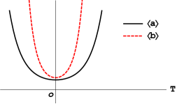
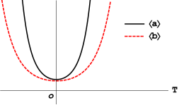
Figure 5: From left to right, expectation values of the scale factors with n=6 and n=8 respectively

An interesting point is, as was to be expected, that both expectation values (34) and (35) coincide when $n=7$. In Figure 5 the time behaviour of $\left\langle a\right\rangle$ and $\left\langle b\right\rangle$ is shown, qualitatively, for different dimensions of the space-time. It should be mentioned that a similar picture four a four-dimensional spacetime was obtained in Ref.[15], where the exponentially decreasing (increasing) classical solutions are replaced by scale factors of a bouncing universe.

From the expression of the expectation values given by the equations (34) and (35), we get for the expansion factor:

$$\Theta_{(n)}=\left[6\frac{1}{\left<a\right>}\frac{d\left<a\right>}{dT}+2(n-4)\frac{1}{\left<b\right>}\frac{d\left<b\right>}{dT}\right]\frac{dT}{dt}.$$ (36)

Now let us consider the behaviour of the expansion factor for $n>5$, shown in Figure 6. It is important to highlight here that the behaviour of $\Theta_{(n)}$, as given by (36), does depend on the space-time dimension, which is distinct from its behaviour at the classical level. The expression of the evolution parameter $T$ as a function of time is obtained from the solution of the Hamiltonian equations (3.2) as $T=\frac{\phi(t)}{\sqrt{2P_{T}}}$, being $P_{T}$ a constant and $\phi(t)$ is given by the classical model. As is expected in the classical approximation, that is, when $t\rightarrow\infty$ and $\xi\rightarrow 0$, we recover the results obtained in Sec. (3.1).

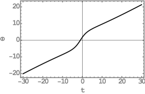
Figure 6: From left to right, expansion factors corresponding to $T(t)$ related to the classical solutions (9) and (10) respectively.

5 The quantization of the $5$-dimensional model

In this section, we present the quantization of the model for $n=5$, taking into consideration the solutions of Eq. (24).

By defining the variables

$$x=2A+B\qquad y=B,$$

and again applying the method of separation of variables, Eq.(24) can be solved similarly to what was done in Sec.(4.2). In this way, the normalized wave function of the universe, for $\omega>0$, will be given by

$$\Psi(x,y,T)=\frac{1}{2\sqrt{\pi}}\left(\frac{\xi}{\xi^{2}+\frac{\omega^{2}}{9}T^{2}}\right)^{\frac{3}{2}}x\;y\exp\left\{-\frac{1}{4}\left[\frac{x^{2}}{\xi-i\frac{\omega}{3}T}+\frac{y^{2}}{\xi+i\frac{\omega}{3}T}\right]\right\},$$

while, for $\omega<0$, we have

$$\Psi(x,y,T)=\frac{1}{2\sqrt{\pi}}\left(\frac{\xi}{\xi^{2}+\frac{\omega^{2}}{9}T^{2}}\right)^{\frac{3}{2}}x\;y\exp\left\{-\frac{1}{4}\left[\frac{x^{2}}{\xi+i\frac{|\omega|}{3}T}+\frac{y^{2}}{\xi-i\frac{|\omega|}{3}T}\right]\right\}.$$ (37)

The expectation value of the three-dimensional and extra-dimensional scale factors will be given, respectively, by

$$\left<a\right>=\frac{1}{4}\left[1+\frac{1}{4}\Sigma(\xi,T^{2})\right]^{2}\exp\left[\frac{\Sigma(\xi,T^{2})}{4}\right],$$ (38)

$$\left<b\right>=\frac{1}{4}\left[1+\Sigma(\xi,T^{2})\right]\exp\left[\frac{\Sigma(\xi,T^{2})}{2}\right],$$ (39)

where we have defined $\Sigma(\xi,T^{2})=\frac{\xi^{2}+\frac{\omega^{2}}{9}T^{2}}{\xi}$. It follows, then, that the expansion factor for $n=5$ calculated from (38) and (39) will be

$$\Theta_{(5)}=\frac{2\omega^{2}}{9\xi}T\left\{\frac{3\left[12+\Sigma(\xi,T^{2})\right]}{2\left[4+\Sigma(\xi,T^{2})\right]}+\frac{3+\Sigma(\xi,T^{2})}{1+\Sigma(\xi,T^{2})}\right\}\frac{dT}{dt},$$ (40)

which exhibits the same profile shown in figure 6 and, as in the previous cases, coincides with classical solutions as $\xi\rightarrow 0$ and $t\rightarrow\infty$.

6 Final remarks

In this work we have investigated the classical and quantum cosmological scenarios predicted by a geometrical scalar-tensor gravitational theory, in an anisotropic $n$-dimensional space-time. At the classical level, we have obtained four different sets of solutions. Two of them represent a dynamical singular universe bearing close resemblance to the well-known Kasner solution . The remaining sets of classical solutions show an interesting picture. In one case we have a non-singular static universe undergoing an expansion regime in the usual three dimensions, while in the extra dimensions we have a contraction. We regard this result as some kind of a $n$-dimensional generalization of the Chodos-Detweiler model [4]. The other case, leading to the opposite behaviour, in which the role of the dimensions are reversed, is also allowed by the field equations.

At the quantum level, we have made use of the approach of quantum cosmology. After carrying out a series of canonical transformations we obtained, after applying the canonical quantization procedure, a Schrödinger-like differential equation for the wave function of the universe. We then found the general solution to this equation and treated separately the cases $n=$ $5$ and $n>5$, which present similar behaviour. In the many-worlds interpretation we found that the expectation values of the scale factors are clearly not singular and, in fact, describe a bouncing universe. In other words, the primordial cosmological singularity is avoided and the whole volume of the universe undergoes a contraction phase, reaches a minimum volume and then starts expanding. When compared with the classical regime, we could say that at the quantum level the two classical solutions are linked to give rise to a non-singular universe, in accordance with previous results [15].

To conclude, let us briefly comment on the role played by the Weyl field in the framework of this geometrical scalar-tensor theory. As is already known, the Weyl transformations preserve the geodesic lines and a number of other geometrical objects, which then implies the physical equivalence of the class of Weyl frames, at the classical level [1]. It is possible to show that there exists a class of Weyl transformations which induce canonical transformations in the reduced Hamiltonian of the original action [18]. However, we still do not know how to extend this classical equivalence to the quantum level, if this is possible at all [19].

Finally, we would like to remark that, with regard to the well-known problem of time in quantum cosmology, it seems appealing to consider that the geometrical nature of the scalar field may lead to a more natural identification of this field with the time parameter that governs the evolution of the quantum variables.

References

References

- [1] T. S. Almeida, M. L. Pucheu, C. Romero, J. B. Formiga, Phys. Rev. D 89, 064047 (2014).
- [2] M. L. Pucheu, F. A. P. Alves-Júnior, A. B. Barreto and C. Romero, Phys. Rev. D 94, 064010 (2016).
- [3] T. Kaluza, Sitz. Preuss. Akad. Wiss. 33, 966 (1921). O. Klein, Z. Phys. 37, 895 (1926). For a review, see L. McAllister and E. Silverstein, Gen. Rel. Grav. 40, 565 (2008). T. Appelquist, A. Chodos and P. Freund, Modern Kaluza-Klein Theories, Addison-Wesley, Menlo Park (1987). P. Collins, A. Martin and E. Squires, Particle Physics and Cosmology, Ch. 13, Wiley, New York (1989). M. Green, J. H. Schwarz and E. Witten, Superstring theory, Cambridge University Press, Cambridge (1987). M. J. Duff, Int. J. Mod. Phys. A 11, 5623 (1996). L. Randall and R. Sundrum, Phys. Rev. Lett. 83, 3370 (1999). L. Randall and R. Sundrum,Phys. Rev. Lett. 83, 4690 (1999). J. M. Overduin and P. S. Wesson, Phys. Rep. 283, 303 (1997). P. S. Wesson, Space-Time-Matter, World Scientific, Singapore (1999).
- [4] A. Chodos and S. Detweiler, Phys. Rev. D 21, 2167-2170 (1980).
- [5] A. A. Garcia and S. Carlip, Phys. Lett. B 645, 101-107 (2007). K. D. Krori, P. Borgohain and K. Das, Gen. Rel. Grav. 22, 791-797 (1990). Ö. Akarsu and T. Dereli, JCAP 2013, 50 (2013).
- [6] For a review see M. Bojowald, Quantum Cosmology, Springer (2011). See also J. J. Halliwell, Introductory lectures on quantum cosmology, in: 7th Jerusalem Winter School for Theoretical Physics: Quantum Cosmology and Baby Universes, Jerusalem (1990), arXiv:0909.2566 [gr-qc]. B. S. DeWitt, Phys. Rev. 160, 1113-1148 (1967).
- [7] C. J. Isham, Canonical quantum gravity and the problem of time, in: 19th International Colloquium on Group Theoretical Methods in Physics (ICGTMP 92) (1992), arXiv:9210011 [gr-qc]. C. Kiefer, Lect. Notes Phys. 541, 158-187 (2000).
- [8] W. F. Blyth and C. J. Isham, Phys. Rev. D 11, 768-778 (1975). N. A. Lemos, Phys. Rev. D 53, 4275-4279 (1996). F. G. Alvarenga, J. C. Fabris, N. A. Lemos and G. A. Monerat, Gen. Rel. Grav. 34, 651-663 (2002).
- [9] H. Farajollahi, M. Farhoudi and H. Shojaie, Int. J. Theor. Phys. 49, 2558-2568 (2010).
- [10] For recent work in this subject see S. Pal, Phys. Rev. D 94, 084023 (2016). C. R. Almeida, A. B. Batista, J. C. Fabris and P. V. Moniz, Quantum cosmology of scalar-tensor theories and self-adjointness, arXiv:1608.08971 [gr-qc].
- [11] P. S. Letelier and J. P. M. Pitelli, Phys. Rev. D 82, 104046 (2010).
- [12] C. Brans and R. H. Dicke, Phys. Rev. 124, 925 (1961).
- [13] H. Weyl, Space, Time, Matter, in Dover Books on Advanced Mathematics, Dover Publications (1952). R. Adler, M. Bazin and M. Schiffer, Introduction to general relativity, in: International series in pure and applied physics, McGraw-Hill (1975). W. Pauli, Theory of Relativity, in: Dover Books on Physics, Dover Publications (1981).
- [14] F. T. Falciano, N. Pinto-Neto and E. S. Santini, Phys. Rev. D 76, 083521 (2007).
- [15] B. Vakili, Phys. Lett. B 718, 34-42 (2012).
- [16] H. Everett, Rev. Mod. Phys. 29, 454-462 (1957).
- [17] F. J. Tipler, Phys. Rep. 137, 231-275 (1986).
- [18] A. B. Barreto, M. L. Pucheu and C. Romero, Weyl frames and canonical transformations in geometrical scalar-tensor theories of gravity, arXiv:1707.08226 [gr-qc].
- [19] See, for instance, A. Anderson, Physics Letters B 305, 67 (1993). Jan Lacki, Studies in History and Philosophy of Modern Physics 35, 317 (2004).