Exploring the Thermal State of the Low-Density Intergalactic Medium at $z=3$ with an Ultra-High Signal-to-Noise QSO Spectrum

Abstract

At low densities the standard ionisation history of the intergalactic medium (IGM) predicts a decreasing temperature of the IGM with decreasing density once hydrogen (and helium) reionisation is complete. Heating the high-redshift, low-density IGM above the temperature expected from photo-heating is difficult, and previous claims of high/rising temperatures in low density regions of the Universe based on the probability density function (PDF) of the opacity in ${\rm Ly\alpha}$ forest data at $2<z<4$ have been met with considerable scepticism, particularly since they appear to be in tension with other constraints on the temperature-density relation (TDR). We utilise here an ultra-high signal-to-noise spectrum of the QSO HE0940-1050 and a novel technique to study the low opacity part of the PDF. We show that there is indeed evidence (at 90% confidence level) that a significant volume fraction of the under-dense regions at $z\sim 3$ has temperatures as high or higher than those at densities comparable to the mean and above. We further demonstrate that this conclusion is nevertheless consistent with measurements of a slope of the TDR in over-dense regions that imply a decreasing temperature with decreasing density, as expected if photo-heating of ionised hydrogen is the dominant heating process. We briefly discuss implications of our findings for the need to invoke either spatial temperature fluctuations, as expected during helium reionization, or additional processes that heat a significant volume fraction of the low-density IGM.

1 Introduction

The thermal state of the IGM in the redshift range $2<z<5$ has received considerable attention over the past two decades. In part, this is due to the sensitivity of IGM temperatures to photo-ionization heating of the low-density IGM during helium (and potentially hydrogen) reionisation (e.g., Hui & Gnedin, 1997; Gnedin & Hui, 1998; Theuns et al., 2001; Theuns et al., 2002; Hui & Haiman, 2003). More generally, IGM temperatures are a potentially powerful diagnostic of galaxy and AGN feedback processes that can have lasting impact on the physical conditions of the low-density IGM.

The primary method to constrain the thermal state of the IGM has been to compare properties of the ${\rm Ly\alpha}$ forest observed in quasar spectra to mock absorption spectra obtained from cosmological hydrodynamical simulations (Haehnelt & Steinmetz, 1998; Schaye et al., 2000; Bolton et al., 2008; Viel et al., 2009; Lidz et al., 2009; Becker et al., 2011; Garzilli et al., 2012; Rudie et al., 2012; Boera et al., 2014; Bolton et al., 2014; Lee et al., 2015). In the numerical simulations the relation between temperature and density at low densities is generally well described by a simple power law of the form

$$T=T_{0}\Delta^{\gamma-1},$$ (1)

where $T_{0}$ is the temperature at the mean density of the Universe, $\Delta$ is the density in units of the mean and $\gamma$ is the index of the relationship. As first shown by Hui & Gnedin (1997), such a power-law relation arises due to the balance of photo-heating and the aggregate effect of recombination and adiabatic cooling due to the expansion of the Universe.

The slope of the temperature-density relation is a potentially powerful tracer of both hydrogen and helium reionization. When atoms are reionized, photon energies in excess of the ionization potential are converted into thermal kinetic energy of the gas. In the simplest picture of an instantaneous and uniform reionization, this photo-ionization heating would impart a uniform amount of energy per atom at all densities, and hence produce a uniform temperature-density relation, i.e. $\gamma=1$. In reality this picture may be significantly complicated due to inhomogeneous reionization and radiative transfer effects, which are likely to produce a multi-valued temperature-density relation during and shortly after reionization (Trac et al., 2008; McQuinn et al., 2009; Compostella et al., 2013). Following hydrogen reionization, the IGM is expected to evolve towards a relatively simple thermal state. High densities are subject to higher recombination rates than low densities, implying multiple heating events, while the cooling is driven by the adiabatic expansion of the Universe at all densities (radiative cooling is negligible at IGM densities). Analytical calculations and hydrodynamical simulations agree that this behaviour leads to an asymptotic value of $\gamma\approx 1.6$ (Hui & Gnedin, 1997). Matters are further complicated by the reionization of HeII, however, which appears to happen significantly later than hydrogen reionization (e.g. Furlanetto & Oh, 2008; Worseck et al., 2011). Helium reionization should flatten again the temperature relation, and is also expected to be spatially inhomogeneous (Abel & Haehnelt, 1999; McQuinn et al., 2009; Meiksin & Tittley, 2012; Compostella et al., 2013; Puchwein et al., 2015). Following helium reionization, the IGM should again evolve towards an asymptotic thermal state with $\gamma\approx 1.6$.

The potential for the thermal evolution of the IGM to shed light on the reionization history has motivated numerous studies aimed at measuring the parameters of the temperature-density relationship $T_{0}$ and $\gamma$. While much progress has been made, the results of these studies have not been fully consistent with each other. In particular, some analyses of the probability distribution function (PDF) of the transmitted ${\rm Ly\alpha}$ flux (Kim et al., 2007) have suggested that the temperature-density relationship could be ‘inverted’ (i.e. $\gamma<1$) at $z=2-4$ (Bolton et al., 2008; Viel et al., 2009; Calura et al., 2012). As noted by Bolton et al. (2008), heating the low-density IGM beyond the temperatures expected from photo-heating is physically challenging within the scenario outlined above. It has been suggested that temperature inhomogeneities during helium reionization could help to explain the discrepancies between observed and simulated PDF (McQuinn et al., 2009; McQuinn et al., 2011). A more speculative possibility is that a non-standard temperature-density relation could result from additional heating at low densities due to plasma instabilities in the IGM following the absorption of TeV photons emitted by blazars that induce pair-production (blazar heating) (Broderick et al., 2012; Chang et al., 2012; Pfrommer et al., 2012). The efficiency of this process is still under debate (Sironi & Giannios, 2014), but blazar heating predicts density-independent (volumetric) heat injection which would effectively lead to an increasing temperature at the lowest densities (Puchwein et al., 2012; Lamberts et al., 2015).

A number of follow-up studies have investigated the extent to which the inferred $\gamma<1$ could be due to systematic errors in the analysis of the ${\rm Ly\alpha}$ forest data. In particular, concerns have been raised about the uncertainty with regard to the continuum placement in quasar spectra (Lee, 2012) and about the estimation of the errors from bootstrapping of the data samples consisting of small chunks of absorption spectra (Rollinde et al., 2013). Skepticism about the claims that the ${\rm Ly\alpha}$ flux PDF suggests a temperature density relation with $\gamma\leq 1$ appeared to be vindicated by careful new measurements of $\gamma$ based on the line-fitting method (Rudie et al., 2012; Bolton et al., 2014), which yield values in the more ’conventional’ range $\gamma\sim 1.5-1.6$. The line-fitting technique is based on the decomposition of the ${\rm Ly\alpha}$ forest into individual Voigt profiles characterised by an HI column density $N_{HI}$ and Doppler parameter $b$. Numerical simulations suggest that the distribution of line parameters in the plane defined by $N_{HI}$ and $b$ and in particular the low-b cut-off are tightly related to the parameters characterising the temperature-density relation (Schaye et al., 1999; Ricotti et al., 2000; Bolton et al., 2014).

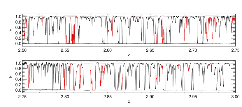
Figure 1: The transmitted flux relative to the continuum level in the ${\rm Ly\alpha}$ forest of HE0940-1050 ($z=3.0932$), as a function of the redshift of ${\rm Ly\alpha}$ absorption. In this work we analyse the region between $z=2.5$ and $z=3.0$, which correspond to rest-frame wavelength of 1040 Å and 1190 Å, respectively. In red we highlight the identified metal lines, which are masked within the region where the fitted absorption is smaller than 0.01 (in units of the continuum, these regions are marked by horizontal red lines above the spectrum). The blue line marks the noise level per pixel estimated by the analysis, while the black dotted lines trace the continuum ($F=1$) and the zero-flux level.

Other methods to characterise the thermal state of the IGM that have been employed adopt the flux power spectrum (McDonald et al., 2000; Zaldarriaga et al., 2001; Croft et al., 2002; Kim et al., 2004) or closely-related statistics, like a decomposition into wavelets (Lidz et al., 2009; Garzilli et al., 2012) or the “curvature” (Becker et al., 2011; Boera et al., 2014, 2016) of the observed flux. The common idea behind these analyses is to characterise the thermal broadening of ${\rm Ly\alpha}$ lines by quantifying the “smoothness” of the ${\rm Ly\alpha}$ forest. Curvature methods have placed strong constraints on the temperature of the IGM at a “characteristic” (over-)density, $\bar{\Delta}(z)$, which evolves with redshift; however, since $T(\bar{\Delta})$ is degenerate in combinations of $T_{0}$ and $\gamma$, the constraints on the shape of the temperature-density relation from these studies have so far been limited (but see Padmanabhan et al., 2015; Boera et al., 2016).

A key challenge in reconciling discrepant constraints on $\gamma$ is to identify the physical properties of the IGM to which these statistics are most sensitive. For example, we will see later that the results from line fitting constrain the temperature density relation only for a rather limited range of densities. Matters are further complicated due to the fact that the thermal part of the broadening of ${\rm Ly\alpha}$ forest absorbers is not only sensitive to the instantaneous temperature, but to the previous thermal history of the IGM. This is due to the effect of thermal pressure on the distribution of the gas, also commonly referred to as pressure smoothing (Peeples et al., 2009a, b; Rorai et al., 2013; Garzilli et al., 2015; Kulkarni et al., 2015).

In this study we will attempt to resolve the apparent tension between flux PDF and line-fitting constraints on $\gamma$ based on two factors: first, that the temperature-density relation at $z\sim 2-3$ may be more complicated than is often assumed, and second, that the two techniques sample the temperatures in different density regimes. To illustrate this, we take advantage of a recently acquired ultra-high S/N spectrum of the bright QSO HE0940-1050 ($z=3.0932$). The high S/N allows us to push our measurements to lower (over)-densities than previous studies and, more importantly, allows us an unprecedented control over the systematic effects due to possible errors in the continuum placement. To take full advantage of the high-quality spectrum we develop a novel analysis method that focuses on the high transmission part of the flux PDF and reduces the impact of continuum placement errors by re-normalizing the PDF to a flux level close to the probability peak (the 95th flux percentile). We further use a suite of state-of-the-art hydrodynamical simulations for which we implement a wide range of temperature density relations in post-processing to put quantitative constraints on a range of different parametrizations of the thermal state of the IGM with Markov chain Monte Carlo (MCMC) techniques.

The paper is structured as follows. We first describe the data in § 2. We then illustrate in § 3 the simulations we use to build our IGM models and describe our different parametrizations of the thermal state of the IGM. Section § 4 presents the details of our analysis method, in particular our approach to dealing with continuum placement uncertainty, the optical depth renormalization, and the estimation of the PDF covariance matrix. Results are presented in § 5 and compared with previous IGM studies in § 6. We discuss the relevance of systematics effect and the interpretation of our results in § 7 and summarize our main findings in § 8.

2 Data

We analyse the spectrum of HE0940-1050 ($z=3.0932$) observed with UVES (Dekker et al., 2000) at the VLT at a resolution of $R\simeq 45000$. This object was chosen as the brightest target in the UVES Large Program (Bergeron et al., 2004). Our final spectrum (herein referred to as the “DEEP” spectrum) was created by combining data from the ESO archive and data from a dedicated program of 43 hours of observation carried out between December 2013 and March 2014. The total integration time amounts to 64.4 hours. This observing time was estimated to be necessary to achieve a sufficient S/N in the ${\rm Ly\alpha}$ forest and to allow the identification of weak CIV and OVI metal lines (see D’Odorico et al., submitted). The S/N in the forest of the reduced spectrum is, on average, 280 per resolution element.

The data has been reduced using the most recent version of the UVES pipeline (Ballester et al., 2000) and a software developed by Cupani et al. (2015b, a) and binned in regular pixels of 2.5 km s^-1. Special care was devoted to minimise the correlation between adjacent pixels of the spectra, which may cause an underestimation of the flux density error (Bonifacio, 2005). Multiple wavelength re-binning of the data was avoided by using the non-merged order spectra (instead of the merged full-range spectra) when combining exposures taken at different epochs.

The final spectrum covers the wavelength range $\lambda\in[3050,7020]$ Å in the vacuum-heliocentric reference system. We will focus here on the ${\rm Ly\alpha}$ forest in the rest-frame wavelength range $\lambda\in[1040,1190]$ Å , which for HE0940-1050 corresponds to the redshift interval $z\in[2.5,3.0]$. These limits are set in order to exclude the regions in proximity of the ${\rm Ly\alpha}$ and ${\rm Ly\beta}$ lines. The continuum-normalized flux in the relevant range is shown in figure 1.

3 Simulations

Model	Parameter	Description
Standard	$T_{0}$	Temp. at $\Delta=1$
	$\gamma$	Index of the TDR
Broken	$\Delta_{b}$	Break density
	$T_{b}$	Temp. at $\Delta=\Delta_{b}$
	$\gamma_{o}$	Index of the TDR at $\Delta>\Delta_{b}$
	$\gamma_{u}$	Index of the TDR at $\Delta<\Delta_{b}$
Discontinuous	$\Delta_{b}$	Discontinuity density
	$T_{+}$	Temp. at $\Delta>\Delta_{b}$
	$T_{-}$	Temp. at $\Delta>\Delta_{b}$
Fluctuations	$Q$	Hot gas filling factor
	$T_{h}$	Temp. at $\Delta=1$ in hot regions
	$T_{c}$	Temp. at $\Delta=1$ in cold regions
	$\gamma_{h}$	Index of the TDR in hot regions
All	$\xi$	Smoothing parameter
	$\bar{F}$	Mean flux

Table 1: Summary of the IGM parameters describing the different thermal models considered in the analysis.

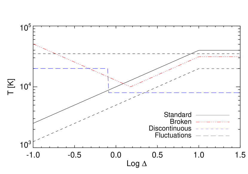
Figure 2: A summary of all the thermal models we consider in our analysis. We first study the standard power-law relationship between temperature and density (black solid) with parameters $T_{0}$ and $\gamma$. We then generalize it by adding a break point at some density $\Delta_{b}$. Such model, shown in red (dotted-dashed line), would have a power-law index $\gamma_{u}$ in underdense regions and a different $\gamma_{o}$ in overdensities ($\Delta>\Delta_{b}$). We also examine the case where the IGM has only two temperatures, below and above some density threshold $\Delta_{t}$. In this plot, this translates into a step-function, depicted in blue (long-dashed line). Last, we implement a model where the IGM is divided into hot isothermal regions and cold regions with $\gamma=1.6$. The division is done independent of density, and the two components are represented by the black dashed lines in the figure.

In order to predict the observed statistical properties of the ${\rm Ly\alpha}$ forest, we used simulated spectra from the set of hydrodynamical simulations described in (Becker et al., 2011, hereafter B11). The simulations were run using the parallel Tree-smoothed particle hydrodynamics (SPH) code GADGET-3, which is an updated version of the publicly available code GADGET-2 (Springel, 2005). The fiducial simulation volume is a 10 Mpc$/h$ periodic box containing $2\times 512^{3}$ gas and dark matter particles. This resolution is chosen specifically to resolve the Ly$\alpha$ forest at high redshift (Bolton & Becker, 2009). The simulations were all started at $z=99$, with initial conditions generated using the transfer function of (Eisenstein & Hu, 1999). The cosmological parameters are $\Omega_{m}=0.26,\Omega_{\lambda}=0.74,\Omega_{b}h^{2}=0.023,h=0.72,\sigma_{8}=0.80,n_{s}=0.96,$ consistent with constraints of the cosmic microwave background from WMAP9 (Reichardt et al., 2009; Jarosik et al., 2011). The IGM is assumed to be of primordial composition with a helium fraction by mass of $Y=0.24$ (Olive & Skillman, 2004). The gravitational softening length was set to 1/30th of the mean linear interparticle spacing and star formation was included using a simplified prescription which converts all gas particles with overdensity $\Delta=\rho/\bar{\rho}>10^{3}$ and temperature $T<10^{5}$ K into collisionless stars. In this work we will only use the outputs at $z=2.735$ .

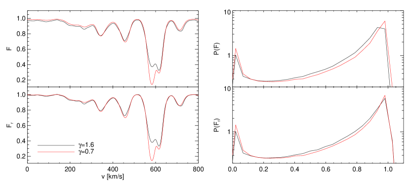
Figure 3: Left column: the continuum regulation procedure applied to a simulated spectrum calculated assuming either $\gamma=1.6$ (black) or $\gamma=0.7$ (red). In the upper panel we plot the flux level in the two models, in the lower panel we show the same spectra after the percentile regulation. The problem of the continuum placement can be understood by carefully looking at the difference between the red and black lines at high fluxes: without regulation (upper panel) the black model ($\gamma=1.6$) is systematically lower than the red one, which could easily lead to an underestimation of the continuum level. With the regulation (lower panel) we impose an alignment in correspondence of the 95th percentile of the flux distribution, regardless of the initial placement of the continuum. Right column: the PDF of the flux $F$ (upper panel) and of the continuum regulated flux $F_{r}$ (lower panel), for the same two IGM models. By imposing the percentile regulation we artificially align the peaks of the distributions, but sensitivity to the thermal state is retained by the overall shape. The advantage of this method is that the regulated PDF is less sensitive to continuum placement errors.

The gas in the simulations is assumed to be optically thin and in ionization equilibrium with a spatially uniform ultraviolet background (UVB). The UVB corresponds to the galaxies and quasars emission model of Haardt & Madau (2001) (hereafter HM01). Hydrogen is reionized at $z=9$ and gas with $\Delta\lesssim 10$ subsequently follows a tight power-law temperature-density relation, $T=T_{0}\Delta^{\gamma-1}$, where $T_{0}$ is the temperature of the IGM at mean density (Hui & Gnedin, 1997; Valageas et al., 2002). As in B11 , the photo-heating rates from HM01 are rescaled by different constant factors, in order to explore a variety of thermal histories. Here we assume the photo-heating rates $\epsilon_{i}=\xi\epsilon_{i}^{HM01}$, where $\epsilon_{i}^{HM01}$ are the HM01 photo-heating rates for species $i=$[HI,HeI,HeII] and $\xi$ is a free parameter. Note that, differently than in B11, we do not consider models where the heating rates are density-dependent. In fact, we vary $\xi$ with the only purpose of varying the degree of pressure smoothing in the IGM, while the TDR is imposed in post-processing. In practice, we only use the hydrodynamical simulation to obtain realistic density and velocity fields. For this reason, we will often refer to $\xi$ as the ’smoothing parameter’. We then impose a specific temperature-density relationship on top of the density distribution, instead of assuming the temperature calculated in the original hydrodynamical simulation. We opt for this strategy in order to explore a wide range of parametrizations of the thermal state of the IGM, at the price of reducing the phase diagram of the gas to a deterministic relation between $T$ and $\rho$. In practice, we find that the native TDR and the matching best-fitting power laws produce nearly identical flux PDFs.

Finally we calculate the optical depth to ${\rm Ly\alpha}$ photons for a set of 1024 synthetic spectra, assuming that the gas is optically thin, taking into account peculiar motions and thermal broadening. For our fiducial spectra we scale the UV background photoionization rate $\Gamma$ in order to match the observed mean flux of the forest at the central redshift of the DEEP spectrum ($\bar{F}_{\rm obs}(z=2.75)=0.7371$, Becker et al., 2013). As described below, however, the mean flux is generally left as a free parameter when fitting the data.

We stress that in this scheme the pressure smoothing and the temperature are set independently. While not entirely physical, this allows us to separate the impact on the Ly$\alpha$ forest from instantaneous temperature, which depends mostly on the heating at the current redshift, from pressure smoothing, which is a result of the integrated interplay between pressure and gravity across the whole thermal history (Gnedin & Hui, 1998).

3.1 Parametrizations of the Thermal State of the IGM

In this section we summarize the thermal models and parameters considered in our analysis. The first parameter is the heating rescaling factor, $\xi$, used on the hydrodynamical simulations, which determines the amount of pressure smoothing. We also include the mean transmitted flux, $\bar{F}$, in the parameter set; however, rather than allow it to vary freely, we impose a Gaussian prior based on the recent measurement of Becker et al. (2013):

$$p(\bar{F})\propto\exp\left[-\frac{(\bar{F}-\bar{F}_{obs})^{2}}{2\sigma_{\bar{F}}^{2}}\right],$$ (2)

where $\bar{F}_{obs}=0.7371$ and $\sigma_{\bar{F}}=0.01$ (which is slightly more conservative than the estimated value).

In order to test whether our findings reproduce previous results in the literature, we first explore the standard power-law TDR parametrized by $T_{0}$ and $\gamma$ (equation 1). The full parameter set describing this model is therefore $\{T_{0},\gamma,\xi,\bar{F}\}$.

Figure 4: The effect of rescaling the optical depth for a selected chunk of the ${\rm Ly\alpha}$ forest of the DEEP spectrum. The plot shows the transformed flux $F_{A}$ after multiplying $\tau$ by a factor $A=1$ (black, original spectrum), 3 (red) and 10 (blue). The spectrum is continuum-regulated before applying the transformation, so that 5% of the pixels have flux above 1, explaining the occasional spikes in the transformed flux. The propagated instrumental errors after the transformation are shown as lighter lines at the bottom, matched by color to the transformed fluxes. The motivation for applying this transformation is that it amplifies fluctuations near the continuum as A increases, while the most absorbed regions, corresponding to high densities, become saturated. This mimics what happens in a denser universe or with a lower amplitude UV background, resembling the ${\rm Ly\alpha}$ forest at higher $z$. In this way we are able to increase our sensitivity to the low density regions of the IGM, which are difficult to probe otherwise.

Next we consider the possibility that underdense regions and overdensities follow different power-law relationships. This model is partly inspired by blazar-heating models, but is mainly designed to provide a simple extension to the simplest power-law model. The relation between temperature and density is described by the expressions

$$T(\Delta)=T_{b}\times\begin{cases}\left(\frac{\Delta}{\Delta_{b}}\right)^{\gamma_{\rm u}-1}&{\rm if\ }\Delta<\Delta_{b},\\ \left(\frac{\Delta}{\Delta_{b}}\right)^{\gamma_{\rm o}-1}&{\rm if\ }\Delta_{b}\leq\Delta<10,\\ {\rm constant}&{\rm if\ }\Delta>10.\end{cases}$$ (3)

Here, $\Delta_{b}$ is the ’break’ density where the transitions between the two regimes occurs. We define a threshold for $\Delta>10$ to avoid unrealistically high temperatures in the high-density regions. This however has little practical effect, as such densities represent a tiny fraction of the ${\rm Ly\alpha}$ forest pixels. The parameters $\gamma_{o}$ and $\gamma_{u}$ define the slope above and below the break density.This parametrization is thus defined by $\{T_{b},\Delta_{b},\gamma_{u},\gamma_{o},\xi,\bar{F}\}$. Note that the standard temperature-density relationship represents a special case of this set of models.

We also calculate a grid of models where the TDR is described by a simple step function:

$$T(\Delta)=\begin{cases}T_{-}&{\rm if}\Delta<\Delta_{b},\\ T_{+}&{\rm if}\Delta\geq\Delta_{b}.\end{cases}$$ (4)

In this model the temperature distribution of the IGM is assumed to be bimodal with only two temperatures, $T_{-}$ in underdense regions and $T_{+}$ in overdensities. Each model is fully defined by the quintuplet $\{T_{+},T_{-},\Delta_{b},\xi,\bar{F}\}$. The motivation behind this simple model is to understand the effect of a density-dependent temperature contrast in its simplest form, rather than assuming some special functional form for the relationship between temperature and density.

Lastly, we consider a set of models including multiple temperatures at a given overdensity. These are meant to mimic the temperature fluctuations expected to be present during helium reionization; however, we do not attempt to capture the full complexity of realistic fluctuations. Instead, we employ a simple model wherein we consider two regions independently of the density. The “hot” regions have a temperature-density relationship defined by $T=T_{h}\Delta^{\gamma_{h}-1}$, where $T_{h}$ is the temperature at mean density, ranging between 15000 K and 35000 K, and $\gamma_{h}\in[0.4,1.3]$ is the index. The “cold” regions are characterised by $T=T_{c}\Delta^{\gamma_{c}-1}$, with $T_{c}\in[5000,15000]$ K and $\gamma_{c}=1.6$, as expected for the IGM long after a reionization event. The fraction of space occupied by the hot region is set by a filling factor, $Q$. All together, the fluctuation models are defined by the parameter set $\{T_{h},\gamma_{h},T_{c},Q,\xi,\bar{F}\}$.

Table 1 recapitulates the four kinds of models analysed in this work and lists the parameters that characterize them. A visual summary of all the thermal models is given in figure 2.

4 Calculation of the Regulated Flux Probability Distribution

In order to exploit the exceptionally high signal-to-noise ratio of our UVES spectrum of HE0940-1050, we apply several modification to the standard flux PDF, which are described in the following sections.

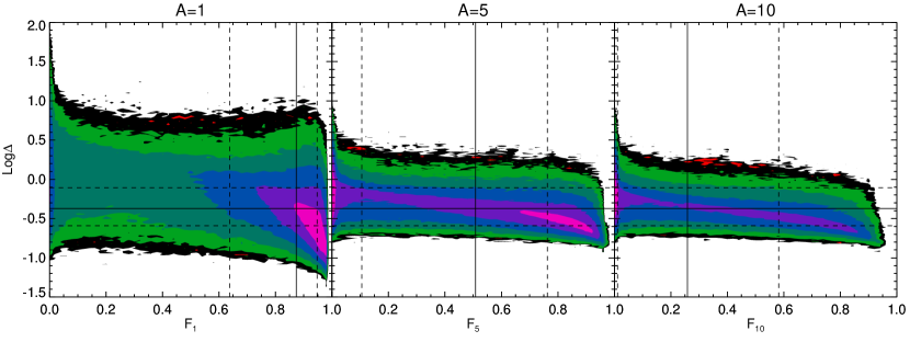
Figure 5: Contour plot of the 2-d distribution of pixels from a simulation in flux-density space. The density pixels, differently than the flux, are calculated in real space. Each color step represents a change in pixel frequency of half a dex (arbitrary units). The simulation has a pressure smoothing parameter of $\xi=0.8$, and the flux used in the left panel is directly taken from the output of the hydrodynamical simulations (i.e. it is not calculated by imposing a temperature-density relationship in post-processing). The thermal parameters fitted to the temperature-density distribution of this simulation are $T_{0}=9600$ K and $\gamma=1.54$ at $z=3$. In the central and right panels we have rescaled the optical depth by a factor 5 and 10, respectively. The vertical (horizontal) black solid line marks the median of the flux (density) distribution, while the dashed lines are drawn in correspondence of the 25th and 75th percentiles. In the right panel, we note that more than 75% of the pixels corresponds to densities below the mean, and more than 75% have a transmitted flux greater than 0.6, occupying the part of the PDF around the peak. Rescaling the optical depth guarantees a more regular distribution of pixels along the flux dimension. Furthermore, with a rescaling factor of 5 or 10, the density distribution is centred below the mean density for any value of the flux. This transformation is thus well suited to study the under-dense regions.

4.1 Noise and Resolution Modelling

Instrumental effects are taken into account by including them in the synthetic spectra. The finite resolution is mimicked by convolving the predicted ${\rm Ly\alpha}$ flux with a Gaussian kernel of width FWHM$\approx 7.2$ km/s, appropriate for a slit aperture of 1”. The simulated spectra are then rebinned onto a regular pixel grid with spacing $\Delta v=2.5$ km/s, as in the DEEP spectrum.

Noise is added to the simulated skewers by the following procedure:

1. We group the pixels of the Deep Spectrum into 50 bins according to the transmitted ${\rm Ly\alpha}$ flux.

2. The instrumental errors of these pixels define 50 different noise distributions, representing the possible value of the noise for a given ${\rm Ly\alpha}$ flux.

3. For each simulated pixel, we randomly select a noise value from one of the 50 subsets above, according to the flux.

Note that this procedure does not capture the wavelength coherence of the noise amplitude (namely, the magnitude of errors should be correlated across adjacent pixels). This does not affect the PDF, however, which retains no information about the spatial distribution of the data. A test of the importance of noise and resolution modelling is presented in appendix A.

4.2 Continuum Uncertainty

Continuum placement is known to be of critical importance in studying the flux PDF of the ${\rm Ly\alpha}$ forest (e.g., Becker et al., 2007; Lee, 2012). Misplacing the continuum level produces a multiplicative shift in the flux values, causing a ’compression’ or a stretching of the PDF which may lead to significant bias on the constraints on $\gamma$. This is of particular concern in the present work, as we aim at characterizing the absorption distribution at high flux levels.

The problem of dealing with continuum uncertainty has been sometimes addressed by trying to estimate it based on the unabsorbed part of the spectrum, on the red side of the ${\rm Ly\alpha}$ emission lines. Typically, such methods are built upon either a power-law extrapolation (e.g., Songaila, 2004), or a Principal Component analysis of a training set of low-redshift quasars (Lee et al., 2012).

Here we adopt a complementary approach that reduces the sensitivity of the flux PDF to the continuum fitting. Assuming that the continuum uncertainty is well approximated by a multiplicative parameter, we can eliminate it by adopting a ’standard’ renormalization based on the spectrum properties. For example, one may choose to set the level $F=1$ at the maximum transmitted flux. Of course, this option is not optimal because the maximum would depend on the noise properties. Alternatively, one can adjust the continuum so that the mean normalized flux matches the observed value at the equivalent redshift (Lee et al., 2012). This ignores variability of the mean flux from one line sight to another, however, which can add significant noise to the measurement. We opt for the following solution. Taking the initial fitted continuum as a starting point, we divide the spectrum into 10 Mpc/$h$ regions. In each region, we find the flux level, $F_{95}$, corresponding to the 95^th percentile of the distribution. We then define the “regulated” flux in each region as $F_{r}=F/F_{95}$, and compute the PDF of $F_{r}$. The advantage of using $F_{95}$ is that the 95-th percentile falls near the peak of the flux PDF for all the IGM models, and it is therefore less noisy than the mean, which falls in a flux interval of low probability.

Realistically, one might expect that spectral features like emission lines would demand a more complex modelling of the continuum uncertainty. Fortunately, however, 10 Mpc$/h$ (equivalent to 1014 km/s at $z\approx 2.75$) is smaller than the typical width of emission lines in quasar spectra. For consistency, the same kind of regulation is applied to the simulated spectra we use to compare the observation with. We perform a test of the effectiveness of the regulation procedure using a set of mock spectra, which is presented in appendix  B. In figure 3 (left column) we report an example of a simulated spectrum before (upper panel) and after (lower panel) the percentile regulation, calculated assuming a thermal model with $\gamma=1.6$ (black) and $\gamma=0.7$ (red). Both models have $T_{0}=15000$ K. Regulation has the effect of aligning the spectra of the two models at high fluxes.

We stress that the statistic obtained in this way (which we will call the regulated flux PDF) is different than the standard PDF analysed in previous works. The right column of Fig. 3 demonstrates that although the regulation aligns the position of the peak, the overall shape retains information about the thermal state.

4.3 Optical Depth Rescaling

${\rm Ly\alpha}$  absorption traces different density ranges at different redshifts. The leading factor in this evolution is the expansion of the Universe. As the overall density decreases, higher overdensities are required to produce the same amount of absorption. This has been quantified in B11, in the context of the the temperature measurement based on the ”curvature” method, by identifying a characteristic density, $\bar{\Delta}$, as a function of redshift, at which the corresponding temperature is a bijective relation with the mean curvature of the ${\rm Ly\alpha}$ forest The existence of $\bar{\Delta}$ has been broadly interpreted suggesting that the ${\rm Ly\alpha}$ probes that particular density. For the redshift range spanned by the DEEP spectrum, the value of the characteristic density calculated in B11 is $\bar{\Delta}=3.35$.

We can partially modify the densities to which the ${\rm Ly\alpha}$ forest is sensitive by implementing a convenient transformation of the flux field. With the aim of studying the low-density range of the IGM, we can artificially enhance the ${\rm Ly\alpha}$ optical depth in each pixel of the spectrum by some arbitrary factor $A$

$$\tau_{A}=A\tau,$$ (5)

where $\tau$ is the observed optical depth. In term of the transmitted flux, this translates into

$$F_{A}=\exp(A\log|F|)=|F|^{A},$$ (6)

where the absolute value is taken to make the transformation well-defined for negative values of the observed flux $F$. All pixels are in this way forced to have a positive flux, however this will not affect the shape of the PDF since negative pixels are generally contained in the bin centred around $F=0$, which is excluded from the analysis (see below).

The effect of this transformation on a section of the DEEP spectrum can be seen in figure 4. Compared to the original ${\rm Ly\alpha}$ flux (black), the rescaled spectra with $A=3$ (red) and $A=10$ (blue) are suppressed at low fluxes, while fluctuations close to the continuum are progressively amplified. At high flux levels, the transformation amplifies both real fluctuations and instrumental noise (shown as thin lines).

It is therefore a distinct advantage to start with a spectrum of exceptional quality like the DEEP spectrum. Figure 5 shows the distribution of pixels from simulated spectra in the flux-density plane, with and without optical-depth rescaling ($A=1,5,10$ from left to right). From this plot it is possible to appreciate the density range probed by the forest at each flux value. The vertical lines mark the 25% (dashed), 50% (solid) and 75% (dashed) percentiles of the flux distribution, giving a different perspective on the effect of the optical depth rescaling. Note however that the flux and the optical depth are defined in velocity space, while the density is defined in real space, so the two quantities are related only in an approximate and statistical sense.

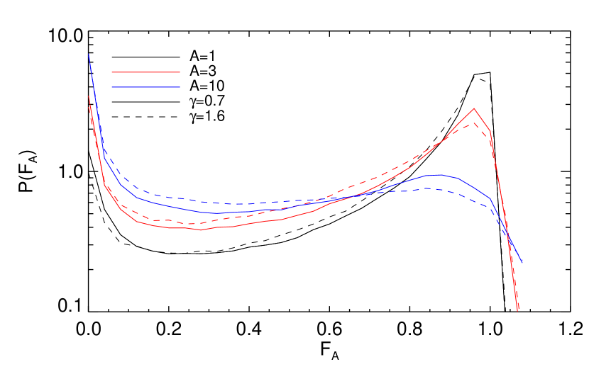
Figure 6: The effect of the optical depth rescaling on the flux PDF, for $A=1,3,10$ (black, red and blue, respectively). The solid lines are calculated from an ”inverted” model with $\gamma=0.7$ and $T_{0}=15000$ K, while the dashed lines represent a model with the same $T_{0}$ but $\gamma_{u}=1.6$. This figure illustrates the advantage of applying the rescaling to the optical depth: as $A$ increases, the structure of the peak of the PDF is better resolved, and the difference between the two models is more evident. In other words, the rescaling corresponds to a convenient rebinning of the flux where the data are more evenly distributed over the bins, in particular near the continuum level.

The impact of the transformation on the flux PDF is illustrated in Fig. 6. A significant fraction of the pixels are contained in the peak of the (untransformed) PDF around $F\approx 0.9$. The structure of this peak is sensitive to the temperature-density relationship at low densities. By applying the optical depth rescaling, the pixels at the peak are redistributed over a larger number of bins, as is clear by comparing the red and the blue curves to the black one, which is obtained without rescaling. This is equivalent to change the binning of the standard PDF in a flux-dependent way, such that the sensitivity at high fluxes is enhanced. In this work we will adopt $A=10$ for the data analysis and to obtain the parameters constraints. We have preliminarily tested that the results are not very sensitive to this choice as long as $A>5$. In the following, we will refer to the PDF of the transformed flux $F_{10}$ as the transformed PDF. We stress that this transformation is applied after the continuum regulation described in § 4.2. The tabulated values of the PDF obtained in this way can be found in Table 2 at the end of this manuscript.

4.4 Metal Line Contamination and Lyman Limit Systems

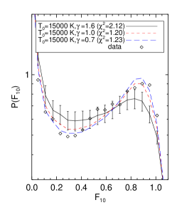
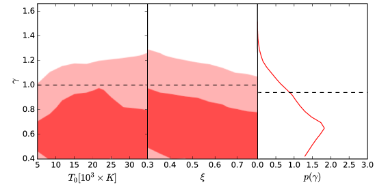
Figure 7: Left panel: PDF of the regulated and transformed flux $F_{10}$ of the DEEP spectrum (black diamonds), compared with the prediction of three different models of the thermal state of the IGM. The standard $\gamma=1.6$ model is shown in black, with errorbars estimated from the simulated spectra as explained in the text. The flat ($\gamma=1$, red dashed) and inverted ($\gamma=0.7$, blue long-dashed) models provide a better fit to the observations, confirming previous findings from the flux PDF. To facilitate the comparison between different models, the lowest-flux bin is not shown. In the legend we provide the values of the reduced $\chi^{2}$ for the three models, calculated taking into account the full covariance and assuming 12 degrees of freedom (16 independent bins and 4 free parameters). The lowest reduced-$\chi^{2}$ value achieved in our parameter grid is $\chi^{2}=0.92$. Right panel: results of the MCMC analysis applying the likelihood in eqn.8 to the PDF of the transformed flux of the DEEP spectrum (where the optical depth is rescaled by $A=10$). The plot shows the 1-$\sigma$ and 2-$\sigma$ confidence levels in the $T_{0}$-$\gamma$ plane (left panel), in the $\xi$-$\gamma$ plane, as well as the marginalized posterior distribution for $\gamma$. The dashed horizontal line marks the level $\gamma=1$, as in an isothermal IGM. We assume a Gaussian prior for the mean flux with mean at $\langle F\rangle=0.7371$ and standard deviation of $\sigma_{\langle F\rangle}=0.01$, based on previous measurements. With these assumptions, the PDF strongly favours an inverted temperature-density relationship if parametrized as a simple power law, consistent with results in the literature (Bolton et al., 2008; Viel et al., 2009; Calura et al., 2012).

Intervening metal lines will tend to modify the flux PDF by increasing the overall opacity of the forest. Rather than attempt to include metals in our simulated spectra, we take advantage of the high quality of the DEEP spectrum by carefully identifying and masking regions contaminated by metal absorption. Our procedure is summarized as follows:

• We first identify all metal absorption systems using lines that fall redward of the ${\rm Ly\alpha}$  emission line.

• We then identify all regions within the forest that are potentially contaminated by metal species associated with these absorbers.

• Finally, remaining lines within the forest that have conspicuously narrow Voigt profile fits (with Doppler parameter $b<8$ km s^-1) are noted and identified where possible.

• Potential ${\rm Ly\alpha}$ lines which do not present compatible higher order Lyman lines (i.e. they are too weak) are also classified, and subsequently identified, as metal lines.

At the end of this process we have a list of lines which we use to define our masking. We perform Voigt profile fits on these lines, and exclude from the analysis all regions where metal absorption amount to more than 1% of the unabsorbed continuum level. This resulted in a cut of about $20\%$ of the total ${\rm Ly\alpha}$ forest, leaving an effective path length of about $\Delta v_{\rm TOT}=31320$ km s^-1.

The list of ions we consider includes: CII, CIV, SiII, SiIII, SiIV, AlII, AlIII, FeII, MgI, MgII, CaII.

The remaining lines are fitted assuming that they are HI ${\rm Ly\alpha}$  absorbers. Among these there are two systems for which the HI column density is estimated to be $N_{HI}>10^{17.2}$ cm^-2, at $z=2.861$ and $z=2.917$. Such systems are classified as Lyman limit systems (LLS) and are known to be self-shielding systems in which the optically thin approximation does not hold (e.g. Fumagalli et al., 2011), so we mask them out from the spectrum.

Because this process is subject to unavoidable uncertainties, we have carried out a test a posteriori where we explicitly show that our results are very weakly sensitive to the removal of metal lines (see appendix C).

4.5 Error Calculation and Likelihood Function

A reliable estimate of the errors on the PDF is not achievable with a single spectrum, let alone the calculation of the full covariance matrix. Therefore we follow a complementary approach in which uncertainties are estimated from the simulations. We extract $n=1000$ mock samples of spectra with the same path length as the DEEP spectrum (31320 km s^-1). Flux PDFs are calculated for these samples, from which we compute the covariance matrix as

$$\Sigma_{i,j}=\frac{1}{n}\sum(p_{i}-\bar{p_{i}})(p_{j}-\bar{p_{j}}),$$ (7)

where $p_{i}$ is the PDF value in the $i-$th flux bin and the sum is performed over the ensemble of 1000 mock samples. We further discuss the calculation and the convergence of the covariance in § 7 and appendix D. In particular, we show that due to cosmic variance we are underestimating variances by $\sim 44\%$, which we correct by multiplying each element of $\Sigma_{i,j}$ by 1.44.

The likelihood is then defined following the standard assumption that the 18 flux bins are distributed as a multivariate Gaussian. Two degrees of freedom are removed by the normalization condition ($\Sigma p_{i}=1$) and by the percentile regulation, hence we remove from the analysis the highest and the lowest of the flux bins. Once this is done, the likelihood is defined as

$$L=\frac{1}{\sqrt{(2\pi)^{k}|\Sigma|}}\exp\left[-\frac{1}{2}(p_{m}-p_{d})^{T}\Sigma^{-1}(p_{m}-p_{d})\right]$$ (8)

where $|\Sigma|$ denotes the determinant of the covariance matrix, $p_{m}$ the PDF array predicted by the model and $p_{d}$ the PDF measured from the data. We stress that both the predicted PDF $p_{m}$ and the covariance matrix are model-dependent.

4.6 MCMC analysis

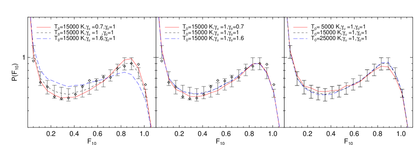
Figure 8: Probability function of the regulated and transformed flux of the deep spectrum (black diamonds), compared with the prediction of IGM models with a temperature-density relationship described by a broken power law. Left panel: the isothermal model (black dashed with errorbars) is taken as a reference, from which we vary the index of the TDR in underdense regions to $\gamma_{u}=0.7,1.6$ (red solid and blue long-dashed, respectively). Analogously to Fig. 7, the inverted and isothermal models provide a better fit to the measured PDF. Central panel: Starting from the isothermal model ($\gamma_{o}=\gamma_{u}=1$, black dashed with errors), we vary the TDR index of overdensities to $\gamma_{o}=0.7$ (red solid) and $\gamma_{o}=1.6$ (blue long-dashed). The three curves are very similar, suggesting that the regulated and transformed PDF is not significantly sensitive to the TDR of densities above the mean. Right Panel: we show the PDF for three isothermal models with temperatures set to $T_{0}=5000$ K (red solid), $T_{0}=15000$ K (black dashed with errors) and $T_{0}=25000$ K (blue long-dashed). The differences are small, demonstrating the insensitivity of the PDF to the overall temperature of the IGM.

We use a Markov-chain Monte Carlo (MCMC) technique to draw constraints from our data. For each set of parameters, we define a regular Cartesian grid (specified in the next section) within the limits set by flat priors and evaluate the likelihood in eq. 8 at each point of the grid. The likelihood is then linearly interpolated between grid points. MCMC chains are obtained using the EmCee package by Foreman-Mackey et al. (2012).

5 Results

We now present the results of fitting the PDF with the thermal models described in § 3.1 and summarized in Figure 2.

5.1 Models with a Standard $T_{0}$-$\gamma$ Parametrization

As previous studies have demonstrated, in the context of the standard $T_{0}$-$\gamma$ parametrization the flux PDF is mostly sensitive to the slope $\gamma$. In Fig. 7 we show the dependence of the PDF of the transformed flux on this parameter (solid lines), compared to the observed values (Black diamonds). We illustrate the case of $\gamma=1.6,1.0,0.7$ in black, red dashed and blue long-dashed, respectively. In this figure, the temperature $T_{0}=15000$ K is fixed, as well as the rescaling of the heating rates in the simulation (i.e. the ’smoothing parameter’) $\xi=0.8$. The isothermal ($\gamma=1$) and the inverted ($\gamma=0.7$) models are most similar to the observed PDF, while the one with $\gamma=1.6$ produce a PDF that is significantly flatter.

We run our MCMC analysis assuming the likelihood reported in eq. 8 and the prior on the mean flux (eq. 2). We use a regular Cartesian parameter grid where the parameters can assume the following values: $\bar{F}\in\{0.7171,0.7271,0.7371,0.7471,0.7571\}$; $\gamma\in\{0.4,0.7,0.85,1,1.15,1.3,1.6,1.9\}$; $T_{0}\in\{5000,15000,25000,35000\}$ ; $\xi\in\{0.3,0.8\}$. We choose small values for the smoothing parameters compared to the model that best match the IGM temperature measured in B11. The choice of a small $\xi$ is conservative as assuming higher smoothing would require lower values of $\gamma$ in order to match the observed PDF, as will become clear when we later investigate the degeneracy between $\xi$ and $\gamma$

The results are summarized in Fig. 7. We present the 68% (dark red) and 95% (light red) confidence levels in the planes defined by the parameters $\gamma$-$T_{0}$ (left panel) and $\gamma$-$\xi$ (middle panel). In the right panel we show the full posterior distribution of $\gamma$, marginalized over all the other parameters. The horizontal dashed line marks the isothermal models ($\gamma=1$). All the models falling below this lines are called ’inverted’. As see in Figure 7, an inverted model is preferred, although an isothermal model is consistent at 1-$\sigma$. This results is consistent with previous works that used the flux PDF (e.g. Bolton et al., 2008; Viel et al., 2009; Calura et al., 2012; Garzilli et al., 2012), and like these it is in tension with constraints on $\gamma$ from different techniques. In the following sections we explore possible models that could resolve this tension.

5.2 Broken-Power Law Models of the Thermal State of the IGM

We next examine broken power-law models of the thermal state of the IGM described in § 3.1. In Fig. 8 we show the effect of the most relevant parameters on the PDF of the transformed flux $F_{10}$. In the models shown in this figure we fix the break density to $\Delta_{b}=1$ (i.e. the mean density), and the parameter regulating the smoothing to $\xi=0.8$. The leftmost panel shows the dependency on the index in underdense regions ($\gamma_{u}$). A value of $\gamma_{u}=0.7$ (inverted) or $\gamma_{u}=1.0$ (flat) provides a much better fit than $\gamma_{u}=1.6$. The results closely resemble those in Fig. 7, suggesting that the PDF is mostly sensitive to the temperature-density relationships at densities below the mean. This is corroborated by the central and right-hand panels of figure 8, which explicitly demonstrate the small role played by the index in the overdense regions ($\gamma_{o}$) and the overall normalization of the temperature-density relation ($T_{0}$) in modifying the transformed PDF.

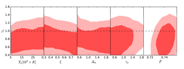
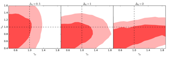
Figure 9: Top row: Results of the MCMC run applying the likelihood in eqn.8 to the PDF of the transformed flux of the deep spectrum ($A=10$), in the parameter space of the broken-power-law model. The plot shows the 68% (dark red) and 95% (light red) confidence levels in the parameter subspaces defined by the power-law index of the TDR in underdense regions $\gamma_{u}$ and, from left to right, the break temperature $T_{b}$, the smoothing parameter $\xi$, the break density $\Delta_{b}$, the slope of the $T$-$\rho$ relationship in overdensities $\gamma_{o}$ and the mean flux $\bar{F}$. A prior on $\bar{F}$ is adopted, as described in the text. The figure shows that, regardless of the choice of the other parameters, an inverted or isothermal $T$-$\rho$ relationship is preferred in underdense regions. There is a mild degeneracy with $\xi$, which means that if the pressure smoothing of the IGM is lower, slightly higher values for $\gamma_{u}$ are tolerated. Bottom row: the 1-$\sigma$ and 2-$\sigma$ confidence levels in the $\gamma_{u}$-$\gamma_{o}$ plane as a function of the break density $\Delta_{b}$. All other parameters are marginalized over. The dashed horizontal (vertical) lines trace the points where $\gamma_{u}=1$ ($\gamma_{o}=1$). The contours broaden in the $\gamma_{o}$ dimension as $\Delta_{b}$ increases, while $\gamma_{u}$ shows the opposite behaviour. If the break point is set to $\Delta_{b}=2$ (right most panel), no constraint can be placed on $\gamma_{o}$, indicating that the transformed flux pdf is not affected by the thermal state of densities above that value.

We carried out a full MCMC analysis in the parameter space defined by $\gamma_{u},\gamma_{o},T_{b},\Delta_{b},\bar{F}$ and $\xi$, adopting the same prior on $\bar{F}$ as in the previous section. The range and spacing of the grid in $\gamma_{u}$, $\gamma_{o}$ and $T_{b}$ is the same as those of $\gamma$ and $T_{0}$ in the previous section, and those of $\bar{F}$ and $\xi$ are unchanged. The break density is varied in the range $\Delta_{b}\in\{0.5,1,1.5,2\}$.

The constraints are presented in Fig. 9. The most important result is that regardless of the choice for the other parameters, the thermal index of underdense regions $\gamma_{u}$ is preferentially inverted or isothermal, with $\gamma_{u}\gtrsim 1.2$ excluded at 2-$\sigma$. The degeneracy of $\gamma_{u}$ with the other parameters is not strong, although lower values of the pressure smoothing do allow a higher $\gamma_{u}$. There is also a slight preference for lower values of $\gamma_{o}$. Note, however, that since the break density $\Delta_{b}$ is a free parameter the physical meaning of $\gamma_{o}$ and $\gamma_{u}$ varies as well.

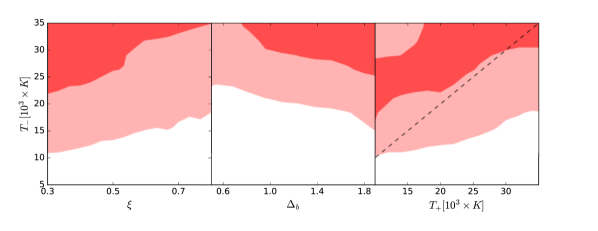
Figure 10: This figure is analogous to Fig. 9, but in the parameter space of the step-function model for the temperature-density relationship. The figure reports the 1-$\sigma$ and 2-$\sigma$ contours in the plane defined by $T_{-}$ and, from left to right, the smoothing parameter $\xi$, the discontinuity density $\Delta_{b}$ and the temperature of overdensities $T_{+}$. The black dashed line in the rightmost panel traces the identity $T_{-}=T_{+}$. The figure, and in particular the right panel, suggest that underdense regions are relatively hot. The required temperature in under-dense regions is comparable or higher then the temperature in overdensities, in the framework of this simple two-temperature model

To illustrate the role played by the break density, we ran three more MCMCs where we fix $\Delta_{b}$ to 0.5,1 and 2. For each run we then calculate the confidence levels in the $\gamma_{u}$-$\gamma_{o}$ plane. The correspondent contours are shown in figure 9. As the break moves from low to higher densities (left to right) there is a clear trend for the contours to shrink in $\gamma_{u}$ and expand in $\gamma_{o}$. We interpret this as the consequence of the different density ranges described by $\gamma_{u}$ and $\gamma_{o}$ in the three cases. For example, in the right panel $\gamma_{o}$ only affects densities above $\Delta_{b}=2$. The fact that the distribution is so broad in $\gamma_{o}$ suggests that the transformed PDF is not sensitive to such overdensities. In the left plot, instead, the constraints on the two indices are relatively similar, suggesting that $\Delta_{b}=0.5$ sits in the density range that prefers an isothermal or inverted $T$-$\rho$ relationship. The central plot lies between the other two cases.

5.3 A Step-Function Model of the Thermal State of the IGM

For the step function given by equation (4), we generate a grid of models where we vary $T_{+}$ and $T_{-}$ between 5000 K and 35000 K, $\Delta_{b}$ between 0.5 and 2, and $\bar{F}$ and $\xi$ between 0.3 and 0.8 with the usual priors and grid spacings.

The most relevant results are shown in figure 10. The contours show the constraints on $T_{-}$ and its degeneracies with the parameters $\xi,\Delta_{b}$ and $T_{+}$. The first point to notice is that cold underdense regions ($T_{-}<15000$ K) are excluded at 2-$\sigma$, independent of the values of other parameters. The degeneracy with the smoothing parameters $\xi$ suggests that the preference for hot underdense regions could be partially mitigated by increasing the fluctuations on small scales through a reduction of the thermal pressure (analogously to § 5.1).

The left panel of Figure 10 illustrates the constraints on the contrast between $T_{-}$ and $T_{+}$. As a reference, we plot the identity line $T_{-}=T_{+}$ as a dashed black line. Nearly the entire 1-$\sigma$ region falls above this line, implying that the PDF demands $T_{+}>T_{-}$. This test supports the general conclusions that the temperatures in underdense regions need to be similar or higher than those in overdensities.

5.4 Temperature Fluctuations

We finally turn towards our simple models for temperature fluctuations. The impacts of the relevant parameters on the transformed PDF are shown in Fig. 11. The figure shows the PDF of two ’uniform’ (i.e. without fluctuations) models of the IGM with $\gamma=1.6,1$ and 0.7 (in black long-dashed, blue and red, respectively); the latter provides a better fit to the data (black diamonds) as shown in previous sections. The blue lines represent two models of temperature fluctuations with the filling factor of the hot gas, $Q$, set to 75% and 50% (dashed and dotted-dashed, respectively). Here the temperature at mean density, $T_{0}$, is 5000 K in the cold regions and 35000 K in the hot regions. The hot regions are assumed to be isothermal and the mean flux of the entire volume is always imposed to be $\bar{F}=0.7371$ by rescaling the UV background. Note that if the filling factor is greater than $50\%$ then the transformed flux PDF becomes similar to the one obtained from an inverted model.

We emphasize that the PDF of a model with temperature fluctuations is not simply a weighted average of the two models characterizing the hot and the cold parts. This would be the case only if the optical depth was not renormalized to match the mean flux constrained by observations. In a mixed model, hot regions are more transmissive than cold regions, due to the lower recombination rate of hydrogen. Compared to the case where the IGM is completely filled with hot, isothermal gas, in a fluctuating medium the transmission of the hot bubbles must compensate the opacity of the cold regions, therefore the UV background must be adjusted such that they are more transparent. The opposite argument could be made for the cold component, which needs to be more opaque when mixed with hot gas. The adjustment of the UV background becomes stronger as the temperature contrast between the hot and cold regions grows. Since this mechanism will increase the number of $F\sim 1$ pixels in hot regions and $F\sim 0$ pixels in cold regions, the net effect on the flux PDF is non trivial. For illustrative purposes we have chosen rather drastic temperature fluctuations, though more realistic models (related to He II reionization, for example), could also be tested with the flux PDF in similar quality data.

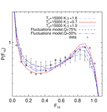
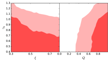
Figure 11: Left panel: PDF of $F_{10}$ from the DEEP spectrum (black diamonds) compared to the prediction of a standard $\gamma=1.6$ model (black long-dashed), an inverted $\gamma=0.7$ model of the thermal state of the IGM (red solid) and two different models with temperature fluctuations. The temperature fluctuation models are built by splitting the simulation box in two parts, one of which has $T_{0}=5000$ K and $\gamma=1.6$ (cold component), the other $T_{0}=35000$ K and $\gamma=1.0$ (hot component). The proportion of the two parts sets the filling factor of the hot component $Q=V_{\rm hot}/(V_{\rm cold}+V_{\rm hot})$. The figure shows in blue the cases where the hot component occupies 75% (dashed) or 50% (dotted-dashed) of the total volume. For comparison, we also show the case of an isothermal IGM, with $T_{0}=15000$ K and $\gamma=1$ (blue solid). We find that models with a strong temperature contrast and high filling factor ($Q>50$%) provide a good fit to the PDF without need of an inverted TDR anywhere. Right panel: 68% and 95% confidence levels in the parameter space that defines the temperature fluctuation models. $\gamma_{h}$ is the slope of the temperature-density relationships in hot regions, $\xi$ is the smoothing parameter and $Q$ is the filling factor of the hot bubbles. The results have been marginalized over the temperature of the hot bubbles $T_{h}$, the temperature in the cold regions $T_{c}$ and the mean flux $\bar{F}$.

We have performed a quantitative parameter analysis for the temperature fluctuations model. We consider the space defined by the quantities $\xi,\bar{F},T_{c},T_{h},\gamma_{h},Q$. We define the parameter grid imposing the cold regions to have $\gamma=1.6$, as expected long after reionization events (Hui & Gnedin, 1997) and temperatures in the set $T_{c}\in\{5000,15000\}$ K. Conversely, the hot regions have higher temperatures $T_{h}\in\{15000,25000,35000\}$ K and a flatter index $\gamma_{h}\in\{0.4,0.7,0.85,1.0,1.15,1.3\}$. The filling factor is set to the values $Q\in\{0,1/4,1/2,3/4,1\}$. Note that the standard models with an inverted temperature-density relationship are a subset of this parameter space, after projection to $Q=1$. Figure 11 presents the most relevant results. The two panels illustrate the degeneracies of $\gamma_{h}$, the thermal index in hot bubbles, with the smoothing parameter $\xi$ and the filling factor $Q$. It is clear that even in the context of temperature fluctuations, hot regions must be filled with inverted or close-to-isothermal gas. The usual degeneracy with $\xi$ applies, confirming the results of the previous sections. Filling factors close to unity are preferred, although only $Q<0.4$ is excluded at 2-$\sigma$. If the volume filling fraction is low, however, lower values of $\gamma$ are required in order to match the transformed PDF.

We stress that these results depend on the simplified description we assume for temperature fluctuations, as well as on our priors on the temperature of cold and hot regions (respectively, flat prior between $T_{c}=5000$ and 15000 K, flat prior between $T_{h}=15000$ and 35000 K). More realistic and theoretically motivated models are needed in order to properly test this scenario. However, this simple exercise reveals that including fluctuations modifies the flux PDF in the direction required by the data.

6 Comparison with Other Techniques

In this section we examine the consistency of our results with other methods that have been used to constrain the thermal state of the IGM using the ${\rm Ly\alpha}$ forest. In particular we will show that the different statistics are sensitive to different density ranges. We first focus on the standard flux PDF and flux power spectrum. We then review the line fitting procedure, and finally demonstrate the consistency of our results with the recent work by Lee et al. (2015) on the flux PDF from the BOSS quasar sample.

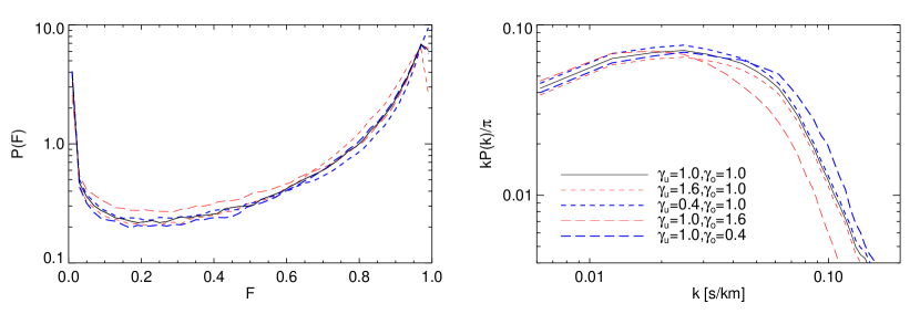
Figure 12: Left panel: the standard flux PDF (not regulated nor transformed) as a function of the indices $\gamma_{u}$ and $\gamma_{o}$. The black solid lines represent a model with $\gamma_{u}=\gamma_{o}=1.0$ . If we vary $\gamma_{u}$ to 1.6 (red dashed) or 0.4 (blue thick dashed) the PDF changes around the peak, at $F\gtrsim 0.6$, while the change occurs at low fluxes for $\gamma_{o}=1.6$ (red long-dashed) and $\gamma_{o}=0.4$ (blue thick long-dashed). Right panel: the flux 1d power spectrum calculated from the same set of models as the upper panel. The shape of the high-$k$ cut-off is only affected by the slope in overdensities (long-dashed lines), while the effect of varying $\gamma_{u}$ (dashed lines) is a small overall shift of the power at all scales. Techniques that rely on the position of the cut-off in the flux power spectrum to determine the temperature are therefore measuring the IGM thermal state at $\Delta\gtrsim 1$. Conversely, the standard flux PDF is sensitive to both regimes, depending on the flux level. However, the shape of the peak ($0.6<F<1.0$) is mostly dependent on the thermal state of underdense regions.

6.1 The Flux PDF and Power Spectrum

We have shown in § 5.2 that the PDF of the transformed flux $F_{10}$ is mostly sensitive to densities around and below the mean. Here we check whether the same argument holds for the standard (non-regulated, non-transformed) flux PDF. Analogous to figure 8, we consider a set of “broken power-law” models and we alternatively vary the TDR above and below the mean density, observing how the PDF responds. In all cases we fix $\Delta_{b}=1$ and $T_{b}=15000$ K. The results are shown in the top panel of figure 12. The black line represents a “reference” model where both indices are set to $\gamma_{u}=\gamma_{o}=1.0$. The long-dashed curves illustrate what happens when the relation between temperature and density in overdensities is made steeper (red, $\gamma_{o}=1.6$) or inverted (blue thick, $\gamma_{u}=0.4$). The PDF changes only at flux levels below $F\lesssim 0.6$, while the peak shape is left almost unchanged. The opposite happens when we vary $\gamma_{u}$ (dashed lines), in which case most of the variation of the PDF occurs around the peak. Therefore the PDF is in principle sensitive to a wide range of densities. We note however that most of the forest pixels lie in underdense regions, i.e. in proximity of the peak, hence we argue that this is the range to which the PDF is mainly sensitive.

The results are qualitatively different for the flux power spectrum, $P(k)$. In the lower panel of Fig. 12 we show $P(k)$ computed for the same broken-power-law thermal models used above. Here, we have computed the power spectrum of the flux contrast, $\delta F$, defined as

$$\delta F=\frac{F}{\langle F\rangle}-1\,,$$ (9)

where $\langle F\rangle$ is the mean flux. The shape of the cut off in $P(k)$ changes only if $\gamma_{o}$ varies (dotted-dashed lines), while the net effect of a variation in $\gamma_{u}$ is just a slight overall renormalization (dashed). This makes sense as the sensitivity of the cutoff shape is dominated by the thermal broadening of absorbers identifiable as lines, while the normalization is set by the amplitude of flux fluctuations at all scales. While the former depends on the temperature at mild overdensities, as it will be obvious from the next section, the latter follows the full mapping of density to ${\rm Ly\alpha}$ flux.

By extension, we infer that any method that uses the smoothness of absorption lines as a proxy for the temperature at these redshifts will most likely be sensitive to the thermal state of high-density regions. Such techniques include the power spectrum, wavelet analysis, curvature and line-fitting. In the next section we examine the line-fitting method explicitly.

6.2 Voigt-Profile Fitting of Absorption Lines

The line-fitting approach decomposes the ${\rm Ly\alpha}$ forest into individual lines fit by Voigt profiles. The fits are then used to construct a 2-d distribution of the H I column densities, $N_{\rm H\,I}$, and Doppler parameters, $b$, of the absorbers. It has been shown (Schaye et al., 1999) that the position and slope of the lower envelope in the $\log N_{\rm H\,I}$-$\log b$ plane is closely related to the thermal parameters $T_{0},\gamma$. Measurements based on this idea, most recently by Rudie et al. (2012) and Bolton et al. (2014), have led to results that are clearly in contrast with a $\gamma<1$ TDR.

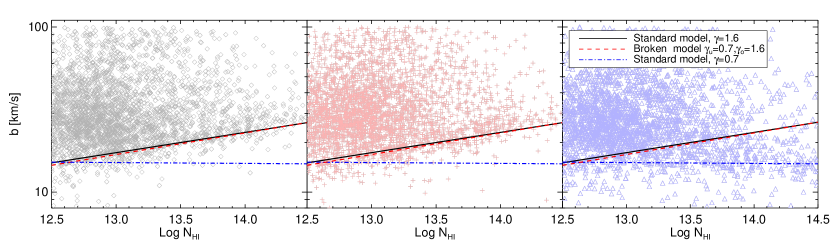
Figure 13: The line distribution in the $b$-$N_{HI}$ plane. The symbols in light colors correspond to individual fitted lines in three IGM models: a standard IGM model with $\gamma=1.6$ and $T_{0}=10000$ K (black, left panel), a broken power-law model with $\gamma_{u}=0.7,\gamma_{o}=1.6,\Delta_{b}=1,T_{b}=10000$ K (middle panel, red) and a standard model with $\gamma=0.7$ and $T_{0}=10000$ K (blue, right panel). The lines represent the fitted power-law to the lower cut-off of the distribution. The fit is done using the algorithm by Schaye et al. (2000) and the lines are matched by color to the models they are derived from. The left and the middle panels show that the line distribution is barely changed if the thermal state of the IGM is modified only in underdense regions. Conversely (right panel), the shape of the cut off is highly sensitive to the temperature-density dependency in overdensities. We therefore conclude that this technique probes the IGM at densities higher than the mean, differently than the PDF.

Following Bolton et al. (2014) we argue that this method preferentially probes the temperature-density relationship at overdense gas. To demonstrate this we consider two models. One is a “standard” model with $T_{0}=10000$ K and $\gamma=1.6$. The other one is a model with inverted underdense regions, i.e. with a break at $\Delta_{b}=1$ and $\gamma_{u}=0.7$. By setting $T_{b}=10000$ K and $\gamma_{o}=1.6$ we ensure that the two models are indistinguishable above the mean density. As a consistency check, we also analyse a standard model with $T_{0}=10000$ K and $\gamma=0.7$.

We then generate a mock sample of spectra for the models, which are forward-modelled as in § 4. vpfit is run on the three datasets to obtain the $N_{\rm H\,I}$-$b$ distributions plotted in Fig. 13. Following Bolton et al. (2014) we consider in the analysis only lines with $12.5<\log N_{HI}<14.5$ (in cm^-2), $8<b<100$ (in km/s) and with relative error on $b$ lower than 50%. We use the algorithm described in Schaye et al. (2000) to fit the lower cutoff of the distributions (coloured lines in the plot), assuming a power-law relation

$$b=b_{0}(N_{HI}/10^{12}cm^{-2})^{\Gamma-1}.$$ (10)

For the standard and broken models we find $\Gamma_{\rm standard}-1=0.146^{+0.033}_{-0.009}$ and $\Gamma_{\rm broken}-1=0.131^{+0.052}_{-0.031}$. In Bolton et al. (2014) they assume the relation $\gamma=1+\xi_{2}/\xi_{1}(\Gamma-1)$, where $\xi_{1}$ and $\xi_{2}$ are determined from an hydrodynamical simulation, giving $\xi_{2}=2.23$ and $\xi_{1}=0.65$. If we follow this assumption, our fit translates into a “measurement” of gamma in these two models of $\gamma_{\rm standard}=1.50^{+0.11}_{-0.03}$ and $\gamma_{\rm broken}=1.45^{+0.17}_{-0.10}$ All errors quoted are 1-$\sigma$. The estimates of $\gamma-1$ in the two models are consistent with each other, and consistent with power-law index of overdensities $\gamma_{o}=1.6$. This test demonstrates that line-fitting techniques do indeed probe the slope of the temperature-density relationship in overdensities, and are largely insensitive to the thermal properties of the underdense regions.

6.3 The BOSS Flux Probability Density Function

Recently, Lee et al. (2015) calculated the ${\rm Ly\alpha}$ flux PDF from a large set of quasars from the BOSS sample and discussed in detail the implications for the thermal parameters. They find that an isothermal or an inverted temperature-density relationship is not statistically consistent with their measurement at any redshift. In this section we present a possible explanation for the tension with our results. The data set employed in their analysis is highly complementary to ours: a large sample of spectra with moderate signal-to-noise ratio and lower resolution compared to a single spectrum with extremely high signal-to-noise ratio. We will investigate now whether the PDF of moderate signal-to-noise and low-resolution data also probes the regime where absorption features are more prominent, i.e. at densities higher than the mean.

To assess this quantitatively, we analyse two sets of mock data, assuming that the IGM is described by a broken model as used in § 5.2. The fiducial model we use has $\gamma_{u}=1$,$\gamma_{o}=1.6$,$\Delta_{b}=1$ and $T_{b}=15000$ K. As a consistency check, we perform the same analysis on a standard model with $T_{0}=15000$ K and $\gamma=1.6$.

For each model, we generate a mock sample with the spectral properties of the BOSS data, as in Lee et al. (2015), and of the DEEP spectrum. In particular we assume that the BOSS-like sample has a path length of 500 ${\rm Ly\alpha}$ forest regions, resolution of R=2000, pixel scale $\Delta v=69$ km/s and a signal to noise of $\sim 10$ per pixel. The DEEP spectrum-like mock sample is constructed as described in § 4.1. We then apply our MCMC analysis to the four flux PDFs (in this case not transformed or regulated) generated from the mock data.

For this test we consider only the bi-dimensional parameter space defined by $T_{0}$ and $\gamma$. Note that this space does not include the ’true’ model in the case where a broken power-law is used. This is done on purpose in order to understand what bias we may get with a wrong parametrization, depending on the properties of the data.

The results of this test are shown in figure 14. On the left we report the results of the consistency check, where we fit $T_{0}$ and $\gamma$ for the fiducial model with $T_{0}=15000$ K and $\gamma=1.6$. Thanks to the large sample size, the BOSS-type data are able to recover the correct parameter values with high precision. The result for the DEEP sample, constructed with the path length of one spectrum, is less accurate but is consistent with the fiducial value. It is also interesting to note the absence of a degeneracy with $T_{0}$.

The case of a broken power law is illustrated on the right. The precision of both samples is significantly degraded. The constraints derived from the DEEP mock sample sit around $\gamma=1$, i.e. the value of $\gamma$ in underdense regions, and a slight degeneracy with $T_{0}$ appears. The BOSS mock instead “measures” a value of $\gamma\approx 1.3$, which is intermediate between the two indices $\gamma_{u}=1$ and $\gamma_{o}=1.6$. From this we infer that the high resolution, high signal-to-noise data are more sensitive to lower densities, as argued above, while the PDF of the moderate-signal-to-noise BOSS data are also sensitive to higher densities. This may partly explain why Lee et al. (2015) favored values of $\gamma\sim 1.5$, while previous PDF analyses using high-resolution data tended to favor lower values of $\gamma$. We stress that in this particular test we are assuming a 2d parameter space ($T_{0}$-$\gamma$), for sake of simplicity. This means that the constraints from the the mock data are more precise than what is achievable with real data in a full analysis.

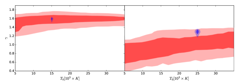
Figure 14: Parameter study of two mock samples of spectra generated from a standard model with $T_{0}=15000$ K and $\gamma=1.6$ (left panel) and on a broken model with $\Delta_{b}=1,T_{b}=1500K,\gamma_{o}=1.6$ and $\gamma_{u}=1$ (right panel). In both cases the smoothing parameter is $\xi=0.8$. One sample is built assuming the path length, signal to noise, pixel scale and resolution of the DEEP spectrum, the other mimicking the path length, noise, pixel scale and resolution of the BOSS sample analysed by Lee et al. (2015). The pdf of the two dataset is calculated for the two models of the thermal state, and then analysed using a set of models where only $T_{0}$ and $\gamma$ are varied. The confidence levels are then obtained through the standard MCMC technique, shown in red (DEEP-like sample) and in blue (BOSS-like sample). The left panel simply confirms that the correct value of $T_{0}$ and $\gamma$ are recovered, and reveals the lack of sensitivity of the PDF from high-quality data to $T_{0}$. The high precision of the BOSS sample is due to the large path length of the data. The right panel illustrates the bias induced on the thermal parameters if the ’true’ IGM is described by a broken model instead of a standard one. A sample with high signal to noise like the DEEP spectrum would be strongly biased towards the values of $\gamma$ in the underdense regions ($\gamma_{u}=1$ in this example), while a noisy and large sample like BOSS would return an intermediate value between $\gamma_{o}$ and $\gamma_{u}$. We interpret this result as a hint that noisier data are less sensitive (in a relative sense) to low densities than high-signal data.

7 Discussion

We have attempted here to shed light on the apparent tension between constraints on the thermal state of the IGM achieved with different techniques. The controversial results yielded by the flux PDF have previously been debated in the context of systematic errors. In particular, some papers showed that misplacing the continuum level could lead to a constraint on $\gamma$ towards lower values (Lee, 2012), or that errors on the flux PDF were underestimated (Rollinde et al., 2013), exaggerating the statistical significance of the claimed inverted temperature-density relationship. Here we paid particular attention to the problem of continuum fitting, by splitting the data into 10 Mpc$/h$ chunks and by applying flux regulation based on the (relatively stable) 95th flux percentile, as described in § 4.2. A test described in appendix B shows how robust the PDF is to continuum uncertainty after this regulation is applied. The only reason the continuum could nevertheless be a source of bias would be if the shape of emission lines in QSO spectra is really different than our assumptions, in particular if the characteristic scale of continuum variations was significantly smaller than 1000 km/s. Given what we know about the characteristics of quasar spectra redwards of the ${\rm Ly\alpha}$ line, and at lower redshift, where the forest is highly transmissive (Scott et al., 2004), this appears unlikely. Furthermore, such small scales fluctuations of the continuum would be problematic for any ${\rm Ly\alpha}$ forest statistic, not just the PDF.

Concerning the estimation of our covariance matrix, with only one spectrum we are unable to estimate the covariance via bootstrap or jackknife techniques. Rollinde et al. (2013) have shown that such methods may underestimate the variance unless the chunks on which the dataset is resampled are larger than $\sim 25$ Å. As explained in § 4.5, however, we used simulated data to calculate the covariance matrix for a forest path length equivalent to the DEEP spectrum. Hence, the question of the accuracy of our errorbars is really a question about the convergence of our simulation with regard to box size. We have performed a convergence test which is described in detail in appendix D. Using two larger boxes of 20 and 40 Mpc$/h$, we find that the PDF is converged well within the estimated errors, while variances are at most about 44% larger in the 40 Mpc/$h$ box compared to the default run. In our analysis we have therefore increased all the elements of the covariance matrix by 44%. We carried out a further convergence test by using larger boxes from a recent set of simulations (Sherwood simulation, Bolton et al, submitted), extending the box size to 80 and 160 Mpc$/h$. The errors on the PDF are converged to $\lesssim 5\%$ for the 160 Mpc$/h$ box.

We also argue that our approach of normalizing the continuum to the 95th percentile of the distribution makes the PDF less subject to large-scale variations. A simple explanation, exact in the linear limit, is to consider large-scale fluctuations as stochastic changes in the mean density along the “local” 10-Mpc$/h$ sight line, i.e. all densities are shifted by some constant. The effect on the forest would be a global renormalization of the transmitted flux, to which the PDF we use is invariant thanks to the regularization. We have in fact verified that not using the percentile regulation significantly degrades the level of convergence with regard to the box size.

8 Conclusions

We have investigated the thermal state of the low-density IGM using the ${\rm Ly\alpha}$ forest of a single quasar spectrum with an exceptional signal-to-noise ratio of 280 per resolution element. As part of the analysis, we have introduced a new technique to address uncertainties due to continuum fitting. We renormalise the flux distribution to a value close to the peak of the flux PDF ( 95th percentile of the flux distribution). We apply this ’flux regulation’ to chunks of ${\rm Ly\alpha}$ forest of 10 (comoving) Mpc$/h$, in order to account for continuum variation on larger scales. Our analysis further employs a rescaling of the ${\rm Ly\alpha}$ optical depth. This gives more emphasis to the high transmission part of the ${\rm Ly\alpha}$ flux PDF and allows us to better probe the low-density IGM. Some information at the high transmissivity end is naturally lost due to the continuum regularization; however, the resulting PDF is virtually free from bias due to continuum placement errors (Fig. 6). Critically, the shape of the PDF of the regularised flux is still very sensitive to the TDR. We have compared the flux PDF obtained from the DEEP spectrum with the predictions of a number of thermal models of the IGM, obtained by imposing different temperature-density relationships on two hydrodynamical simulations with fixed density and velocity fields. We have considered four different parametrizations for the TDR, starting with the standard simple power law relation characterised by $T_{0}$ and$\gamma$. We then have moved to more complex parametrisation with broken power laws and steps in the TDR, to see whether in this way the tension between the constraints on the thermal states estimated from the PDF and from other statistics of the ${\rm Ly\alpha}$ forest could be reconciled.

For each of these parametrizations we have used Bayesian MCMC techniques to obtain constraints. Our main results can be summarized as follows.

• In our analysis of the flux PDF based on the regularised and rescaled flux we find, assuming a power law TDR, that $\gamma>1$ is excluded at 90% confidence levels and $\gamma>1.1$ at 95% confidence level, after marginalization over the remaining parameters. This results is consistent with previous measurement obtained from the PDF, but in contrast with other methods. The fact that we still find this for our very high SN spectrum and with our continuum regulation suggests that this discrepancy is not solely attributable to errors in the continuum placement.

• We have tested a ’broken’ power law TDR in which densities below and above a threshold $\Delta_{b}$ have different power-law indices $\gamma_{o}$ and $\gamma_{u}$. Our constraints for this model suggest a flat or inverted TDR around and below the mean density ($\Delta\lesssim 2$) provide a good fit to the measured PDF.

• If the thermal state is assumed to be characterized by two temperatures $T_{+}$ and $T_{-}$, assigned to densities above and below $\Delta_{b}$, then models with $T_{+}\lesssim T_{-}$ are favoured. This suggests that the evidence for relative hot gas in underdense regions is robust with respect to the particular choice of the parametrization.

• The fit to the observed PDF is also improved by our model of temperature fluctuations as could be possibly induced by HeII reionization. Our MCMC analysis for this model suggests again that a significant fraction of the volume ($Q>0.4$) must be filled with hot gas characterized by a flat or inverted TDR.

• Regardless of the parametrization chosen, low values for the pressure smoothing parameters $\xi$ provide a better fit to the PDF and broaden the allowed range for the TDR parameters. This result is consistent with independent constraints on the smoothing from quasar pairs (Rorai et al, submitted).

• We have shown that the flux power spectrum and the lower Doppler parameter cut-off in the $N_{HI}$-$b$ distribution are mainly sensitive to the thermal state of the IGM at mean density and above, differently than the high-transmissivity part of the PDF that we analyse here. Hence, the flux PDF on one side and the the power spectrum and the line-fitting techniques on the other side are primarily sensitive to sufficiently different densities that their measurements are not actually in tension if a more flexible parametrisation is chosen to characterise the thermal state of the IGM.

Concerning the degeneracy between $\gamma$ and the smoothing parameter $\xi$, it is interesting to note that a recent analysis of Rorai et al. (2016, submitted) of the flux correlation in QSO pairs provided a first direct estimate of pressure smoothing. As Rorai et al. point out the density field may also be different than that in our simulations due to the effect of primordial magnetic fields or a different small scale matter power spectrum than we have assumed here. Although the amplitude of the matter power spectrum on intermediate scales as characterised by $\sigma_{8}$ is now known with reasonably high precision (Planck Collaboration et al., 2015), no constraints are yet available for the matter power spectrum on scales below $\sim 1$ Mpc. If the matter power spectrum is different than we assumed on small scales, this would certainly affect the ${\rm Ly\alpha}$ forest statistics and in particular the PDF which is more sensitive to low-densities in the linear and quasi-linear regime.

The discrepancy of the flux PDF from that expected if photo-heating of hydrogen dominates has been previously attributed to additional heating sources like blazars or to non-equilibrium and radiative transfer effects during HeII reionization. Our analysis of the flux PDF of the ${\rm Ly\alpha}$ forest region in the ultra-high SN spectrum of HE0940-1050 confirms that, regardless of the particular parametrization we choose, for a significant ($\gtrsim$ 50%) volume fraction of the IGM the temperature in under dense regions appears to be at least as high as the temperature at mean density and above. Both incomplete helium reionization and blazar heating appear to be broadly consistent with this result and more detailed simulations will be needed to investigate if this still holds if either process is simulated more realistically.

Finally, we emphasize that the results presented in this paper were obtained from a single sight line. The next obvious step would be to extend our methodology to a larger sample of quasars. Although the signal to noise level of the DEEP spectrum is unmatched, our results suggest that more standard high-quality high S/N data may nevertheless yield precise constraints for a wide range of densities. We further advocate in particular the use of multiple and complementary ${\rm Ly\alpha}$ forest statistics, in order to discriminate between the different thermal models of the IGM that were presented in this paper.

Appendix A Sensitivity to the Noise and Resolution Estimates

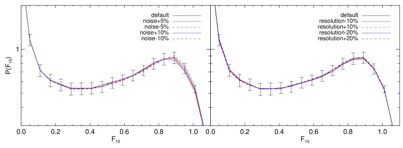
Figure 15: The effect of varying the assumptions with regard to noise and resolution: in the upper panel we plot the transformed and regulated PDF calculated from a model which uses the noise level estimated from the pipeline (black solid) or in the case where it is increased (solid lines) or decreased (dashed lines) by 5% (red) and 10% (blue); in the lower panel we show an analogous test where we compare the PDF computed assuming the default resolution of 7.2 km/s (black solid) with the cases where the resolution is increased (dashed) or decreased (solid) by 10% (red) or 20% (blue). All the lines in this plot are derived from a thermal model with $\xi=0.8$,$\gamma=1,T_{0}=15000$ K and $\bar{F}=0.7371$. The changes induced on the PDF are in all cases much smaller than the statistical errors calculated for the default model.

The transformation of the optical depth defined in § 4.3 amplifies the noise in proximity of the continuum. We therefore need to demonstrate that the transformed PDF of the ${\rm Ly\alpha}$ flux is not strongly sensitive to the noise and resolution modelling when we employ an optical-depth rescaling factor as high as $A=10$. We verify this by calculating the PDF after varying our assumptions with regard to noise level and resolution. We tested variations of 5%-10% for the noise level and of 10%-20% for the spectral resolution. The results are shown in figure 15. The test is performed for a single model with $\xi=0.8$,$\gamma=1,T_{0}=15000$ K and $\bar{F}=0.7371$. The differences between the PDF of the modified and the default models are in all cases much smaller than the statistical errors. We argue that this is a consequence of the extremely high signal to noise ratio of the spectrum, and of the fact that the ${\rm Ly\alpha}$ absorption features are fully resolved at the spectral resolution of UVES.

Appendix B Mock Test of the Continuum Regulation

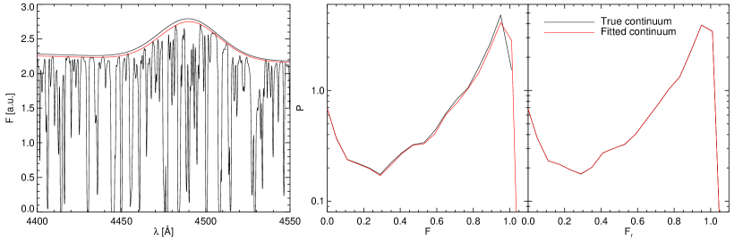
Figure 16: Left panel: example of a mock spectrum used in our continuum regulation test (flux in arbitrary units). The true continuum of this spectrum is plotted as a black line, while the fitted version is shown in red. The fitted continuum is systematically lower than the original one, but the slope and the shape of mock emission lines are recovered with good accuracy. Middle panel: the standard flux PDF of the ${\rm Ly\alpha}$ forest of the sample of mock spectra assuming the true continuum (black) or the fitted one (red). The continuum misplacement clearly results in an overestimation of the PDF toward high values of the flux, as a consequence of using the high transmission regions as anchor points for the fit. Right panel: the same as the middle panel but using the percentile-regulated flux. The two PDFs are now practically identical, suggesting that on scales of 10 Mpc$/h$, to which our procedure is applied, the continuum error is well approximated by a normalization uncertainty.

The 95-percentile regulation ensures invariance to a rigid rescaling of the continuum of the 10-Mpc$/h$ chunks. In reality, the true continuum could differ from the fitted one in more complicated ways, particularly if emission lines are present. To assess the robustness of our regulation method, we perform the following test employing mock data.

• We generate 10 mock ${\rm Ly\alpha}$ forest spectra with path length comparable to the real spectrum. For this we have concatenated the (periodic) simulated spectra at the location of local minima and maxima, such such that the flux level at the juncture differs by less then 0.01. This ensures that the spectra are practically $C^{1}$ continuous.

• Each of these spectra are multiplied by a continuum level with a slope defined by $C\propto z^{\alpha}$, where $z$ is the ${\rm Ly\alpha}$ absorption redshift and $\alpha$ is randomly chosen between -1.2 and 0.3 . We randomly add between zero and five Gaussian emission lines, whose width is drawn between $\sigma=$800 km/s and $\sigma=$2000 km/s and with maximum heights between 5% to 25% of the continuum level. Finally, we add the same amount of noise as estimated for the DEEP spectrum.

• One of us (RFC) then fitted the continuum using a similar technique applied to the DEEP spectrum, without a priori knowledge of the true continuum. An example is shown in figure 16

• Finally, we calculated the PDF of the ${\rm Ly\alpha}$ transmitted flux using the true and fitted continua for both the raw normalized fluxes and for the regulated fluxes. The results are illustrated in figure 16.

We find that the continuum fitting does increase the probability of the highest flux levels, which can be seen in the last bin of the flux of Fig. 16. Although the effect is very small, it could lead to a significant bias in the estimate of $\gamma$. However, once we have applied the 95-percentile regulation, the difference between the true and the recovered distributions are negligible.

Appendix C The Effect of Contamination by Metal Lines and LLS

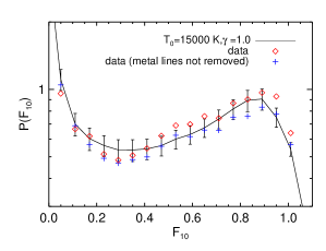
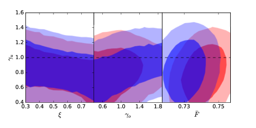
Figure 17: The effect of contamination from metal lines and LLS: on the left we plot the transformed and regulated PDF with metals and LLS identified and masked (default case, red diamonds) and calculated from all the pixels in the ${\rm Ly\alpha}$ forest (red crosses), before removing contaminants. The black solid lines represents an isothermal model with $T_{0}=15000$ K, $\xi=0.8$ and the mean flux set to $\bar{F}=0.7371$ (i.e. the observed value at z=$2.75$). In the right panel we plot the contours of the 68% and 95% confidence levels in the parameter space of the broken TDR, projected onto the $\xi$-$\gamma_{u}$,$\gamma_{o}$-$\gamma_{u}$ and $\bar{F}$-$\gamma_{u}$ planes. The contours are calculated by running the MCMC analysis on the data with metal masked (default, red) and on the whole, unmasked spectrum (blue).

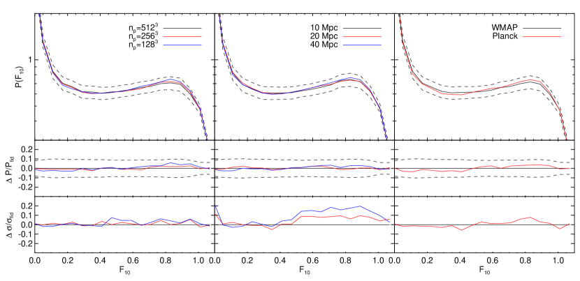
Figure 18: Convergence test of the transformed and regulated PDF in our hydrodynamical simulations. We show the effect of resolution (left), box size (middle) and cosmology (right). The upper panels show the PDFs of the fiducial runs and of the test runs, in the middle panels we plot the relative deviation of the PDF from the fiducial simulation, compared to the square root of the diagonal element of the covariance matrix (dashed black lines). In the bottom panel we present instead the relative deviation of the diagonal errors. All the simulations used in this test have the smoothing parameter set to $\xi=1.45$. Left panels: results for three simulations with box size 10 Mpc$/h$ with 512³ (fiducial,black), $256^{3}$ (red) 128³ (blue) gas particles are shown. The PDF and the diagonal errors are converged to a few-percent level. Central panels: The fiducial model is a 10 Mpc$/h$ simulation with 128³ gas particles. We compare its PDF and the diagonal errors to those calculated from a 20 Mpc$/h$ simulation with 256³ gas particles (in red), and a 40 Mpc$/h$ simulation with 512³ particles (in blue). While the mean PDF is converged to a small fraction of the estimated uncertainty, the error themselves show a significant variation when the box size is increased. We correct the covariance matrix in our analysis to take this into account (see text). Right panels: The black model uses the same cosmological parameter we have used throughout this paper, while the red curves are calculated assuming the best-fit values from the first data release of Planck (Ade et al., 2014). The differences are always significantly smaller than the statistical errors.

The exceptional data quality of the DEEP spectrum facilitates the identification of narrow lines in the forest caused by metal absorption and of strong lines caused systems with a large hydrogen column density (see § 4.4 for a description of our approach in removing metal lines and LLS). There is however an unavoidable uncertainty due to the possibility of blending of the ${\rm Ly\alpha}$ forest absorption with these contaminants.

In this appendix we assess the impact of contamination by showing the difference in the PDF and in the results if the presence of metals and LLS were totally ignored.

In the left panel of Fig. 17 we show the transformed and regulated PDF from the data as it was used in our default analysis (red diamonds) and calculated from all the pixels in the ${\rm Ly\alpha}$ forest of the spectrum (blue crosses), also those that were flagged as contaminated. The PDF of an isothermal model is plotted in black for reference. We see indeed a slight change in the shape of the PDF, with in particular a decrease in the occurrence of high-flux pixels. This is a natural consequence of the increase in the average opacity when metal lines are included. The right panel of figure 17 explicitly reports the bias in the constraints we would get in the case of the broken TDR: the most relevant bias is the shift of the mean flux towards lower values in the contaminated case (blue contours) compared to the default simulation (red), and the broadening of the constraints on the slope $\gamma_{o}$ in over-dense regions. The posterior distribution of $\gamma_{u}$ and its degeneracy with the pressure smoothing parameter $\xi$ are only marginally affected, demonstrating the robustness of our results with respect to this possible source of bias.

We argue that since metal lines and LLS have high optical depths, they mainly alter the shape of the PDF at low values of $F$ (and of course of $F_{10}$). The modification induced on the high-flux part of the PDF is mainly attributable to the change of the overall mean flux which follows the removal of many dark pixels.

Appendix D Convergence tests

We verify the convergence of the transformed flux PDF with respect to resolution and box size of the simulations. We use as reference a simulation with box size of 10 Mpc$/h$ and $512^{3}$ gas particles. We then compare the transformed PDF of this default run with those calculated from two simulations with the same box size and $256^{3}$ and $128^{3}$ gas particles, respectively. All the simulations have been performed with a pressure smoothing parameter of $\xi=1.45$, and for this test we use the actual temperature distribution of the hydrodynamical simulation, instead of the post-processed temperature-density relation. The parameters obtained by fitting the phase space are $T_{0}=14000$ K and $\gamma=1.54$ at $z=3$. We then calculate the PDF of the transformed flux $F_{10}$, after applying the continuum regulation. We also calculate the covariance matrix of the same statistic. The result of this test is shown in the left panel of figure 18. The PDF is converged within the estimated errorbars at all flux levels. The errors, taken as the square root of the diagonal elements of the covariance matrix, are also reasonably converged, with a difference of at most 10% between the $256^{3}$ and the $512^{3}$ simulations.

An analogous test is carried out in order to verify the convergence with respect to the box size of the simulations. We use three simulations with box size 10,20 and 40 Mpc$/h$ with $128^{3},256^{3}$ and $512^{3}$ gas particles respectively. With this choice the three simulations have the same resolution, so that we can isolate the effect of volume sampling alone. The central panel of figure 18 shows that the PDF is converged at the few percent level, significantly better than the estimated statistical uncertainty. The standard deviations are less well converged than in the resolution test, revealing the effect of cosmic variance in the simulations with larger box size. We find that variations could be as large as as 20%. We therefore correct the standard deviations in our simulations by a factor $\iota=1.2$, which corresponds to a correction to variances of $\iota^{2}=1.44$. For this reason, we multiply each element of the covariance matrix employed in the likelihood in formula 8 by 1.44.

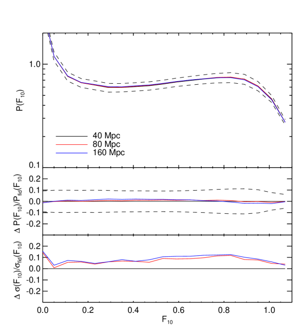
Figure 19: Same as the central panel of Fig. 18, but considering three runs from the Sherwood set of simulations (Bolton et al., 2016). The boxes are 40,80 and 160 Mpc$/h$ of size with $2\times,512^{3},1024^{3},2048^{3}$ particles respectively, which matches the resolutions of the simulation shown in Fig. 18. Compared to the previous test on smaller boxes, the convergence of the errors is significantly improved, down to a level of 5% at most for the 80 Mpc$/h$ box (we remind the reader that the $F_{10}=0$ bin is excluded from the analyses). We reckon that this level of convergence is satisfactory for the degree of precision of this work, and a slight change in our covariance estimate would not qualitatively modify any of our conclusions.

Since error estimation of the flux PDF is known to be a delicate process in the flux PDF (Rollinde et al., 2013) we extend our convergence test to bigger boxes taking advantage of a new set of high-resolution hydrodynamical runs, the Sherwood simulations (Bolton et al., 2016). These simulations were run using the Gadget-3 code (Springel, 2005), assuming the UV background and photoheating rates from the model of Haardt & Madau (2012). More details can be found in Bolton et al. (submitted) and Keating et al. (2016). We used three simulations with size 40,80 and 160 Mpc$/h$ and $512^{3},1024^{3},2048^{3}$ gas particles, respectively. The resolution of these runs is the same as that of simulations used for the previous convergence test, although the cosmology and the assumption on the thermal history are slightly different. The results are shown in figure 19. The convergence achieved at 40 Mpc$/h$ is excellent with respect to the PDF, and better than 10% for the estimated errors. This should be sufficient for our purposes.

Appendix E Dependence on Cosmological Parameters

We also test the dependency of the flux PDF of cosmological parameters, by comparing our default simulations, which assumes the best-fit cosmological parameters of the WMAP data, to a simulated box run with the cosmological parameters as constrained from the first data release of Planck (Ade et al., 2014): $\Omega_{m}=0.274,\Omega_{b}=0.0457,n_{s}=0.968,H_{0}=70.2$ km s^-1 Mpc^-1 and $\sigma_{8}=0.816$. The result is shown in the rightmost panel of figure 18: the variation to the change in cosmology is always less significant than the estimated errors.

Appendix F Tabulated Values of the PDF

$\langle F_{10}^{(a)}\rangle$	$P(F_{10})^{(b)}$	$\Delta P(F_{10})^{(c)}$
-0.01	4.205	0.410
0.05	0.958	0.119
0.11	0.665	0.081
0.17	0.617	0.070
0.23	0.514	0.060
0.29	0.483	0.059
0.35	0.507	0.060
0.41	0.545	0.057
0.47	0.620	0.057
0.53	0.690	0.058
0.59	0.699	0.060
0.65	0.759	0.064
0.71	0.743	0.071
0.77	0.868	0.082
0.83	0.902	0.097
0.89	0.967	0.098
0.95	0.930	0.074
1.01	0.638	0.038
1.07	0.239	0.019

Table 2: Tabulated values of the PDF of the regulated and transformed flux. (a) Central value of the flux bin. (b) Probability density of $F_{10}$. (c) Error on the PDF estimated from a fiducial simulation (see text).

We report in Table 2 the values of the PDF of the regulated and transformed flux from HE0940-1050. We emphasize that for a meaningful comparison all data properties should be included in the models (see § 4.1). In order to add noise to the synthetic spectra, we suggest to add Gaussian fluctuations to each pixel (which should be 2.5 km/s wide), using the amplitude given by the flux-dependent expression $\sigma(F)=\sqrt{\sigma_{0}^{2}+F(\sigma_{c}^{2}-\sigma_{0}^{2})}$, with $\sigma_{0}=0.0028$ and $\sigma_{c}=0.0088$. We have checked that this formula represents an excellent approximation of the more comprehensive treatment described in § 4.1. Continuum regulation and optical-depth rescaling procedures must be applied to simulated spectra consistently with what we have done in this paper (§ 4.2, 4.3). Finally, note that the given errors are estimated from a fiducial simulation with $T_{0}=15000$ K and $\gamma=1$ and should be used only for illustrative purposes. A rigorous statistical comparison with the PDF data requires the prediction of the full covariance matrix from the model, as explained in § 4.5.

References

- Abel & Haehnelt (1999) Abel T., Haehnelt M. G., 1999, ApJ, 520, L13
- Ade et al. (2014) Ade P., et al., 2014, Astron.Astrophys.
- Ballester et al. (2000) Ballester P., Modigliani A., Boitquin O., Cristiani S., Hanuschik R., Kaufer A., Wolf S., 2000, The Messenger, 101, 31
- Becker et al. (2007) Becker G. D., Rauch M., Sargent W. L. W., 2007, ApJ, 662, 72
- Becker et al. (2011) Becker G. D., Bolton J. S., Haehnelt M. G., Sargent W. L. W., 2011, MNRAS, 410, 1096
- Becker et al. (2013) Becker G. D., Hewett P. C., Worseck G., Prochaska J. X., 2013, MNRAS, 430, 2067
- Bergeron et al. (2004) Bergeron J., et al., 2004, The Messenger, 118, 40
- Boera et al. (2014) Boera E., Murphy M. T., Becker G. D., Bolton J. S., 2014, MNRAS, 441, 1916
- Boera et al. (2016) Boera E., Murphy M. T., Becker G. D., Bolton J. S., 2016, MNRAS, 456, L79
- Bolton & Becker (2009) Bolton J. S., Becker G. D., 2009, MNRAS, 398, L26
- Bolton et al. (2008) Bolton J. S., Viel M., Kim T., Haehnelt M. G., Carswell R. F., 2008, MNRAS, 386, 1131
- Bolton et al. (2014) Bolton J. S., Becker G. D., Haehnelt M. G., Viel M., 2014, MNRAS, 438, 2499
- Bolton et al. (2016) Bolton J. S., Puchwein E., Sijacki D., Haehnelt M. G., Kim T.-S., Meiksin A., Regan J. A., Viel M., 2016, preprint, (arXiv:1605.03462)
- Bonifacio (2005) Bonifacio P., 2005, Memorie della Societa Astronomica Italiana Supplementi, 8, 114
- Broderick et al. (2012) Broderick A. E., Chang P., Pfrommer C., 2012, ApJ, 752, 22
- Calura et al. (2012) Calura F., Tescari E., D’Odorico V., Viel M., Cristiani S., Kim T.-S., Bolton J. S., 2012, MNRAS, 422, 3019
- Chang et al. (2012) Chang P., Broderick A. E., Pfrommer C., 2012, ApJ, 752, 23
- Compostella et al. (2013) Compostella M., Cantalupo S., Porciani C., 2013, MNRAS, 435, 3169
- Croft et al. (2002) Croft R. A. C., Weinberg D. H., Bolte M., Burles S., Hernquist L., Katz N., Kirkman D., Tytler D., 2002, ApJ, 581, 20
- Cupani et al. (2015a) Cupani G., et al., 2015a, Mem. Soc. Astron. Italiana, 86, 502
- Cupani et al. (2015b) Cupani G., et al., 2015b, in Taylor A. R., Rosolowsky E., eds, Astronomical Society of the Pacific Conference Series Vol. 495, Astronomical Data Analysis Software an Systems XXIV (ADASS XXIV). p. 289 (arXiv:1509.04901)
- Dekker et al. (2000) Dekker H., D’Odorico S., Kaufer A., Delabre B., Kotzlowski H., 2000, in Iye M., Moorwood A. F., eds, Proc. SPIE Vol. 4008, Optical and IR Telescope Instrumentation and Detectors. pp 534–545
- Eisenstein & Hu (1999) Eisenstein D. J., Hu W., 1999, ApJ, 511, 5
- Foreman-Mackey et al. (2012) Foreman-Mackey D., Hogg D. W., Lang D., Goodman J., 2012, preprint, (arXiv:1202.3665)
- Fumagalli et al. (2011) Fumagalli M., Prochaska J. X., Kasen D., Dekel A., Ceverino D., Primack J. R., 2011, MNRAS, 418, 1796
- Furlanetto & Oh (2008) Furlanetto S. R., Oh S. P., 2008, ApJ, 681, 1
- Garzilli et al. (2012) Garzilli A., Bolton J. S., Kim T.-S., Leach S., Viel M., 2012, MNRAS, 424, 1723
- Garzilli et al. (2015) Garzilli A., Theuns T., Schaye J., 2015, MNRAS, 450, 1465
- Gnedin & Hui (1998) Gnedin N. Y., Hui L., 1998, MNRAS, 296, 44
- Haardt & Madau (2001) Haardt F., Madau P., 2001, in Neumann D. M., Tran J. T. V., eds, Clusters of Galaxies and the High Redshift Universe Observed in X-rays. (arXiv:astro-ph/0106018)
- Haardt & Madau (2012) Haardt F., Madau P., 2012, ApJ, 746, 125
- Haehnelt & Steinmetz (1998) Haehnelt M. G., Steinmetz M., 1998, MNRAS, 298, L21
- Hui & Gnedin (1997) Hui L., Gnedin N. Y., 1997, MNRAS, 292, 27
- Hui & Haiman (2003) Hui L., Haiman Z., 2003, ApJ, 596, 9
- Jarosik et al. (2011) Jarosik N., et al., 2011, ApJS, 192, 14
- Keating et al. (2016) Keating L. C., Puchwein E., Haehnelt M. G., Bird S., Bolton J. S., 2016, preprint, (arXiv:1603.03332)
- Kim et al. (2004) Kim T.-S., Viel M., Haehnelt M. G., Carswell R. F., Cristiani S., 2004, MNRAS, 347, 355
- Kim et al. (2007) Kim T.-S., Bolton J. S., Viel M., Haehnelt M. G., Carswell R. F., 2007, MNRAS, 382, 1657
- Kulkarni et al. (2015) Kulkarni G., Hennawi J. F., Oñorbe J., Rorai A., Springel V., 2015, ApJ, 812, 30
- Lamberts et al. (2015) Lamberts A., Chang P., Pfrommer C., Puchwein E., Broderick A. E., Shalaby M., 2015, ApJ, 811, 19
- Lee (2012) Lee K.-G., 2012, ApJ, 753, 136
- Lee et al. (2012) Lee K.-G., Suzuki N., Spergel D. N., 2012, AJ, 143, 51
- Lee et al. (2015) Lee K.-G., et al., 2015, ApJ, 799, 196
- Lidz et al. (2009) Lidz A., Faucher-Giguere C., Dall’Aglio A., McQuinn M., Fechner C., Zaldarriaga M., Hernquist L., Dutta S., 2009, preprint, (arXiv:0909.5210)
- McDonald et al. (2000) McDonald P., Miralda-Escudé J., Rauch M., Sargent W. L. W., Barlow T. A., Cen R., Ostriker J. P., 2000, ApJ, 543, 1
- McQuinn et al. (2009) McQuinn M., Lidz A., Zaldarriaga M., Hernquist L., Hopkins P. F., Dutta S., Faucher-Giguère C.-A., 2009, ApJ, 694, 842
- McQuinn et al. (2011) McQuinn M., Hernquist L., Lidz A., Zaldarriaga M., 2011, MNRAS, 415, 977
- Meiksin & Tittley (2012) Meiksin A., Tittley E. R., 2012, MNRAS, 423, 7
- Olive & Skillman (2004) Olive K. A., Skillman E. D., 2004, ApJ, 617, 29
- Padmanabhan et al. (2015) Padmanabhan H., Srianand R., Choudhury T. R., 2015, MNRAS, 450, L29
- Peeples et al. (2009a) Peeples M. S., Weinberg D. H., Davé R., Fardal M. A., Katz N., 2009a, preprint, (arXiv:0910.0256)
- Peeples et al. (2009b) Peeples M. S., Weinberg D. H., Davé R., Fardal M. A., Katz N., 2009b, preprint, (arXiv:0910.0250)
- Pfrommer et al. (2012) Pfrommer C., Chang P., Broderick A. E., 2012, ApJ, 752, 24
- Planck Collaboration et al. (2015) Planck Collaboration et al., 2015, preprint, (arXiv:1502.01589)
- Puchwein et al. (2012) Puchwein E., Pfrommer C., Springel V., Broderick A. E., Chang P., 2012, MNRAS, 423, 149
- Puchwein et al. (2015) Puchwein E., Bolton J. S., Haehnelt M. G., Madau P., Becker G. D., Haardt F., 2015, MNRAS, 450, 4081
- Reichardt et al. (2009) Reichardt C. L., et al., 2009, ApJ, 694, 1200
- Ricotti et al. (2000) Ricotti M., Gnedin N. Y., Shull J. M., 2000, ApJ, 534, 41
- Rollinde et al. (2013) Rollinde E., Theuns T., Schaye J., Pâris I., Petitjean P., 2013, MNRAS, 428, 540
- Rorai et al. (2013) Rorai A., Hennawi J. F., White M., 2013, ApJ, 775, 81
- Rudie et al. (2012) Rudie G. C., Steidel C. C., Pettini M., 2012, ApJ, 757, L30
- Schaye et al. (1999) Schaye J., Theuns T., Leonard A., Efstathiou G., 1999, MNRAS, 310, 57
- Schaye et al. (2000) Schaye J., Theuns T., Rauch M., Efstathiou G., Sargent W. L. W., 2000, MNRAS, 318, 817
- Scott et al. (2004) Scott J. E., Kriss G. A., Brotherton M., Green R. F., Hutchings J., Shull J. M., Zheng W., 2004, ApJ, 615, 135
- Sironi & Giannios (2014) Sironi L., Giannios D., 2014, ApJ, 787, 49
- Songaila (2004) Songaila A., 2004, AJ, 127, 2598
- Springel (2005) Springel V., 2005, MNRAS, 364, 1105
- Theuns et al. (2001) Theuns T., Mo H. J., Schaye J., 2001, MNRAS, 321, 450
- Theuns et al. (2002) Theuns T., Schaye J., Zaroubi S., Kim T., Tzanavaris P., Carswell B., 2002, ApJ, 567, L103
- Trac et al. (2008) Trac H., Cen R., Loeb A., 2008, ApJ, 689, L81
- Valageas et al. (2002) Valageas P., Schaeffer R., Silk J., 2002, A&A, 388, 741
- Viel et al. (2009) Viel M., Bolton J. S., Haehnelt M. G., 2009, MNRAS, 399, L39
- Worseck et al. (2011) Worseck G., et al., 2011, ApJ, 733, L24
- Zaldarriaga et al. (2001) Zaldarriaga M., Hui L., Tegmark M., 2001, ApJ, 557, 519