Graphene-based three-body amplification of photon heat tunneling

Abstract

We consider a three slabs configuration including two non-doped single layer graphene on insulating silicon dioxide (G/SiO₂) substrates and one non-doped suspended single layer graphene (SG). The suspended layer is placed between two G/SiO₂ layers. Without SG layer, the heat flux has maximum at Plasmon frequency supported by the G/SiO₂ slabs. In three slabs configuration, the photon heat tunneling is amplified between two G/SiO₂ layers significantly, only for specific range of vacuum gap between SG layer and G/SiO₂ layers and Plasmon frequency, due to the coupling of modes between each G/SiO₂ layer and SG layer. Since, the SG layer is a single atomic layer, the photon heat tunneling assisted by this configuration does not depend on the thickness of middle layer and in consequence, it can enable novel applications for nanoscale thermal management.

I Introduction

In any material, there will be spontaneous electrical and magnetic moments that originate from quantum and thermal fluctuations. These fluctuating moments produce fluctuating electromagnetic fields inside and outside the material. One can calculate these fluctuating fields by adding a fluctuating induction terms to the Maxwell’s equation Landau and Lifshitz (1960). Lifshitz has found the fields inside and outside the materials by using the fluctuation-dissipation theorem Lifshitz (1955). Since 1930, London has realized that quantum mechanical fluctuations of electric dipole moments could give rise to the force between bodies separated by macroscopic distances (van der Waals force) London (1930). Abrikosova et al. have made the first direct measurements of the van der Waals force between macroscopic bodies Abrikosova and Derjaguin (1953). The energy flow between two half spaces has been found using Lifshitz’s method by using the Poynting vector rather than the Maxwell stress tensor Loomis and Maris (1994). Sipe has developed new Green function formalism for calculating fields generated by sources in the presence of a multilayer geometry Sipe (1987). Narayanaswamy et al. have found a relation between cross-spectral densities of electromagnetic fields in thermal equilibrium and dyadic Green functions of the vector Helmholtz equation Narayanaswamy and Chen (2010) and then generalized it to thermal non-equilibrium effects (i.e., when the objects are at different temperatures) and introduced a Green function formalism of energy and momentum transfer in fluctuational electrodynamics Narayanaswamy and Zheng (2014).
But, what will be the force and heat transfer between bodies separated by nanometer distances? Several groups Loomis and Maris (1994); Polder and Vanhove (1971); Mulet et al. (2002); Fu and Zhang (2006) have shown that when the gap distance, $d$ between bodies becomes very small, the near-field heat transfer varies as $d^{-2}$. By using nonlocal dielectric function it has been shown that, the $d^{-2}$ dependence would disappear for $d<0.1$ nanometer (nm)Chapuis et al. (2008),Volokitin and Persson (2001) but generally speaking, the nonlocal effects has little influence on the predicted heat flux for $d>0.1$ nmChapuis et al. (2008). Basu et al. have considered two semi-infinite plates separated by a vacuum gap of finite width, especially for $0.1<d<100$ nm, and studied the dependency of maximum heat flux to the dielectric function and vacuum gap width Basu and Zhang (2009). In addition at subwavelength gap (i.e., in near field regime), it has been shown that, a significant increment of heat flux results from the evanescent photons which remain confined near the surface of the materials Joulain et al. (2005); Volokitin and Persson (2007); Kittle et al. (2005); Hu et al. (2008); Rousseau et al. (2009); Shen et al. (2009); Kralik et al. (2011); Ottens et al. (2011). Messina et al., have considered a metal-like (ML) medium layer (with width, $\delta$) between two silicon carbide (SiC) layers (with width, $d$) and studied the amplification of photon heat tunneling in this structure Messina et al. (2012). They have shown that, only for $0.05<\delta<0.2$ micrometer $(\mu m)$ and $0.05<d<0.3$ $\mu m$, the amplification was occurredMessina et al. (2012). The amplification of photon heat has opened new possibilities for development some technologies such as, thermophotovoltaic conversion devices DiMatteo et al. (2001); Narayanaswamy and Chen (2003), Plasmon assisted nano-photolithography Srituravanich et al. (2004) and infrared sensing and spectroscopy Wilde et al. (2006); Jones and Raschke (2012).
In the present work, we consider three-body configuration including a non-doped suspended single layer graphene (SG) which is placed between two non-doped single layer graphene on silicon dioxide (G/SiO₂) substrates. At first, we calculate the photon heat tunneling between two G/SiO₂ structure and show: how the heat flow depends on the value of gap ($d$) between these layers and frequency of filed ($\omega$). Then, we place the SG layer between these two G/SiO₂ structures, when the heat flux on SG layer is zero, and show that, the heat transfer between G/SiO₂ substrates is amplified only for specific range of vacuum gap between SG and each G/SiO₂ substrate i.e, $d$ and Plasmon frquency. The structure of the article is as follows: in section II the analytical calculation method of dielectric constant of non-doped graphene and evanescent part of heat transfer will be presented. In section III the result and discussion and in section IV the summary will be provided, respectively.

II Analytical calculations

In this section of article, we provide the calculation method of dielectric constant and evanescent part of heat transfer.

II.1 Dielectric constant of undoped graphene

The expectation value of an arbitrary observable $\hat{A}$ under the influence of a probe potential of the form:

$$\hat{V}(t)=\hat{B}F(t)\theta[t-t_{0}]$$ (1)

with $\hat{B}$ being an observable,$F(t)$ a scalar function of time, and $\theta(t)$ the Heaviside step function, can be written as:

$${\textlangle\delta\hat{A}(t)\textrangle}=\int_{-\infty}^{+\infty}{\frac{d\omega}{2\pi}}{\chi_{AB}(\omega)}{F(\omega)}{e^{-i\omega t}}$$ (2)

where $F(\omega)$ is Fourier transformation of $F(t)$ and $\chi_{AB}(\omega)$ is complex-valued generalized susceptibility, which is equal to:

$${\chi_{AB}(\omega)}={-i}\int_{0}^{+\infty}{d}{t^{\prime}}{\textlangle[\hat{A}(t^{\prime}),\hat{B}]\textrangle}_{eq}{e^{(i\omega t^{\prime}-0t^{\prime})}}$$ (3)

This quantity can be written with a slightly different, more convenient, notation as Nagaosa (1999); Scholz (2013):

$$\chi(\vec{q},\omega)=4\sum_{\alpha,\alpha^{\prime}=\pm 1}\int{\frac{d^{2}\vec{k}}{4\pi^{2}}}{\frac{({n_{F}(\alpha E_{k})}-{n_{F}(\alpha^{\prime}E_{k+q})})}{(\omega+\alpha E_{k}-\alpha^{\prime}E_{k+q}+i\epsilon)}}F_{\alpha\alpha^{\prime}}(\vec{q},\vec{k})$$ (4)

where $\epsilon=0^{+}$, $\alpha(\alpha^{\prime})$ index of band, and

$$F_{\alpha\alpha^{\prime}}(\vec{q},\vec{k})={\frac{1}{2}}(1+\alpha\alpha^{\prime}{\frac{k^{2}+\vec{k}.\vec{q}}{{k}\mid{\vec{k}+\vec{q}}\mid})}$$ (5)

$$n_{F}(E)=[e^{\beta\hbar\omega}+1]^{-1}$$ (6)

where $\beta=(k_{B}T)^{-1}$ , with $T$ the temperature and $k_{B}$ the Boltzmann constant. If $\theta$ is angle between $\vec{k}$ and $\vec{q}$ then

$$F_{\alpha\alpha^{\prime}}(\vec{q},\vec{k})={\frac{1}{2}}(1+\alpha\alpha^{\prime}{\frac{k+q\cos(\theta)}{\mid{\vec{k}+\vec{q}}\mid})}$$ (7)

By changing the variable, $u=(1+\alpha\alpha^{\prime}{\frac{k+q\cos(\theta)}{\mid{\vec{k}+\vec{q}}\mid}})$ and using the below relations:

$$\omega-k=\mid{\vec{k}+\vec{q}}\mid$$ (8)

$$\cos(\theta)={\frac{(k+q\cos(thetaθ))}{(\omega-k)}}$$ (9)

$$\sin(\theta)=\pm{\frac{1}{2kq}}\sqrt{{4k^{2}q^{2}-(\omega^{2}-2\omega k-q^{2})^{2}}}$$ (10)

The imaginary part of $\chi(\vec{q},\omega)$ becomes (for $q<\omega$):

$$Im(\chi(\vec{q},\omega))={\frac{-1}{\pi\sqrt{\omega^{2}-q^{2}}}}\int_{\frac{\omega-q}{2}}^{\frac{\omega+q}{2}}{d}{k}\sqrt{q^{2}-\omega^{2}+4k\omega-4k^{2}}$$ (11)

But, $\sqrt{q^{2}-\omega^{2}+4k\omega-4k^{2}}=\sqrt{q^{2}-(\omega+2k)^{2}}$, and if $x\equiv\mid\vec{q}\mid/\mid\vec{k_{F}}\mid$ and $\upsilon=\omega/E_{F}$, it can be shownScholz (2013); Hwang and Sarma (2007):

$$Im(\chi(\vec{q},\omega))=-{\frac{x^{2}\theta(\upsilon-x)}{4\sqrt{\upsilon^{2}-x^{2}}}},q<\omega$$ (12)

$$Im(\chi(\vec{q},\omega))=0,q>\omega$$ (13)

Also, based on the Kramers-Kronig relation, the relation between $Im(\chi(\vec{q},\omega))$ and $Re(\chi(\vec{q},\omega))$ is as followsScholz (2013):

$$Re(\chi(\vec{q},\omega))={\frac{2}{\pi}}P\int_{0}^{\infty}{d}{\omega^{\prime}}{\frac{\omega^{\prime}Im(\chi(\vec{q},\omega))}{\omega^{\prime^{2}}-\omega^{2}}}$$ (14)

where, $P$ means principle vlaue. ThereforeScholz (2013):

$$Re(\chi(\vec{q},\omega))=-{\frac{x^{2}\theta(x-\upsilon)}{4\sqrt{x^{2}-\upsilon^{2}}}},q>\omega$$ (15)

$$Re(\chi(\vec{q},\omega))=0,q<\omega$$ (16)

However, based on the random phase approximation, the relation between dielectric constant $\varepsilon(\vec{q},\omega)$ and susceptibility $\chi(\vec{q},\omega)$ can be written as Hwang and Sarma (2007):

$$\varepsilon(\vec{q},\omega)=1-V(q)\chi(\vec{q},\omega)$$ (17)

where, $V(q)=2\pi e^{2}/\kappa q$ is the two dimensional Coulomb interaction. Therefore Hwang and Sarma (2007),

$$Re(\chi(\vec{q},\omega))=1+{\frac{e^{2}}{2\varepsilon_{0}\varepsilon_{r}}}(1+x\theta(x\pm\upsilon)/(4\sqrt{x^{2}-\upsilon^{2}}))$$ (18)

$$Im(\chi(\vec{q},\omega))={\frac{e^{2}}{2\varepsilon_{0}\varepsilon_{r}}}x\theta(\pm\upsilon-x)/(4\sqrt{\upsilon^{2}-x^{2}})$$ (19)

Now, if $\upsilon>x$ then:

$$Re(\chi(\vec{q},\omega))=1+{\frac{e^{2}}{2\varepsilon_{0}\varepsilon_{r}}}$$ (20)

$$Im(\chi(\vec{q},\omega))={\frac{e^{2}}{2\varepsilon_{0}\varepsilon_{r}}}x/(4\sqrt{\upsilon^{2}-x^{2}})$$ (21)

II.2 Evanescent photon heat tunneling

The three-body configuration is shown in Fig.1. First, we consider the structure without intermediate suspended graphene layer. We assume that the materials are nonmagnetic.

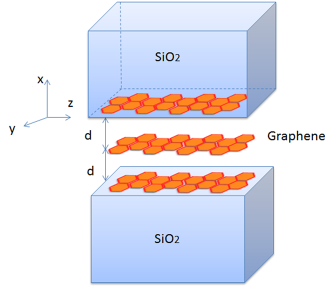
Figure 1: Schematic of three-body configuration for photon heat tunneling calculation.

It is obvious that, the electric and magnetic field that are generated by the component of the fluctuating induction $\vec{g}(\vec{r},t)$ hold in the Maxwell’s equationsLoomis and Maris (1994)

$$\nabla\times\vec{E}(\vec{r},\omega)=i{\frac{\omega}{c}}\vec{H}(\vec{r},\omega)$$ (22)

$$\nabla\times\vec{H}(\vec{r},\omega)=-i{\frac{\omega}{c}}\vec{E}(\vec{r},\omega)-i{\frac{\omega}{c}}\vec{g}(\vec{r},t)$$ (23)

We can write the fields in terms of Fourier components as:

$$\vec{E}={\int_{-\infty}^{+\infty}}{\vec{a}}(\vec{k})e^{i\vec{k}.\vec{r}}{d}{\vec{k}},\vec{H}={\frac{c}{\omega}}{\int_{-\infty}^{+\infty}}{\vec{k}}{\times}{\vec{a}}(\vec{k})e^{i\vec{k}.\vec{r}}{d}{\vec{k}}$$ (24)

and $\vec{g}$ as:

$$\vec{g}={\int_{-\infty}^{+\infty}}{\vec{g}}(\vec{k})e^{i\vec{k}.\vec{r}}{d}{\vec{k}}$$ (25)

By substituting Eqs.24 and 25 in Eqs.22 and 23, and defining the below vectors:

$$\vec{k}_{\pm}=\vec{q}+\pm s_{1}\hat{x},\vec{q}=k_{y}\hat{y}+k_{z}\hat{z},s_{1}=\sqrt{\omega^{2}\varepsilon_{SiO_{2}}-q^{2}}$$ (26)

$$\hat{s}=\hat{q}\times\hat{x},\hat{p}_{\pm}=k^{-1}(q\hat{x}\mp s_{1}\hat{q})$$ (27)

$$\vec{\rho}=y\hat{y}+z\hat{z}$$ (28)

The transverse and parallel component of filed become Loomis and Maris (1994):

$$\vec{E}^{\perp}=\int{\frac{i\pi\omega^{SiO_{2}}{t_{10}^{\perp}}}{c^{2}q^{2}s_{1}}}exp[i\vec{q}.\vec{\rho}+ipx]\times[\vec{g}(\vec{k}).(\vec{q}\times\hat{x})](\vec{q}\times\hat{x})d^{2}q$$ (29)

$$\vec{E}^{\parallel}=\int{\frac{i\pi\omega^{SiO_{2}}{t_{10}^{\parallel}}}{{\sqrt{\varepsilon_{SiO_{2}}}}q^{2}s_{1}}}exp[i\vec{q}.\vec{\rho}+ipx]\times[q^{2}g_{x}(\vec{k})-s_{1}(\vec{q}.\vec{g}(\vec{k}))](q^{2}\hat{x}-p\vec{q}]d^{2}q$$ (30)

where,$\vec{E}^{\perp}$ and $\vec{E}^{\parallel}$ arise from the wave polarized perpendicular and parallel to the plane of incidence, respectively and $t_{10}^{\perp}$ and $t_{10}^{\parallel}$ are the transmission coefficients when the electric field is perpendicular and parallel to the plane of incidence, respectively. It can be shown that, if the vacuum width $d$ satisfies in the below equation:

$$d\ll\frac{c}{2\omega\sqrt{\mid(1-\varepsilon_{1,2})\mid}}$$ (31)

where, $\varepsilon_{1,2}=\varepsilon_{SiO_{2}}$ or $\varepsilon_{SG}$. The evanescent part of the heat flow, $P_{ev}$, is equal toLoomis and Maris (1994):

$$P_{ev}={\frac{\hbar}{\pi^{2}d^{2}}}\int_{0}^{\infty}\omega d\omega(n_{B}(E,T_{1})-n_{B}(E,T_{2}))\times\int_{0}^{\infty}\gamma d\gamma{\frac{Im(\varepsilon_{1})Im(\varepsilon_{2})}{(\mid(\varepsilon_{1}+1)(\varepsilon_{2}+1)-(\varepsilon_{1}-1)(\varepsilon_{2}-1)e^{-\gamma}\mid)^{2}}}e^{-\gamma}$$ (32)

Where, $\gamma=-2p\omega d/c$ and $n_{B}(E,T_{i})=[e^{β\hbar\omega}-1]^{-1}$. If the SG layer is absent, then:

$$X\equiv\int_{0}^{\infty}\gamma d\gamma{\frac{Im(\varepsilon_{1})Im(\varepsilon_{2})}{(\mid(\varepsilon_{1}+1)(\varepsilon_{2}+1)-(\varepsilon_{1}-1)(\varepsilon_{2}-1)e^{-\gamma}\mid)^{2}}}e^{-\gamma}=\int_{0}^{\infty}\gamma d\gamma{\frac{Im(\varepsilon_{1})Im(\varepsilon_{2})}{(\mid(\varepsilon_{G/SiO_{2}}+1)^{2}-(\varepsilon_{G/SiO_{2}}-1)^{2}e^{-\gamma}\mid)^{2}}}e^{-\gamma}$$ (33)

$X$ is radiative heat flux in the near-field and after normalization is shown by$X^{*}$Basu and Zhang (2009). In next section, we will use Eqs.20, 21, 32 and 33 for calculating $P_{ev}$ .

III Numerical calculations and discussion

As an example, let us to consider two materials both with $-5\leq Re(\varepsilon)\leq 5$ and $0.001\leq Im(\varepsilon)\leq 10$ and study the heat flux between them. Fig.2(a) and (b) shows the normalized heat flux $X^{*}$ when the thickness of gap $d$ is equal to zero and 10 nm, respectively.

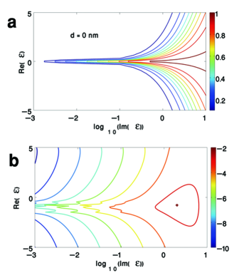
Figure 2: (Color online) (a) Contour plot of $X^{*}$as a function of $Re(\varepsilon)$ and $Im(\varepsilon)$ at $d=0nm$ and (b) $log_{10}(X^{*})$ at $d=10nm$.

As Fig.2 shows, only for specific values of $Re(\varepsilon)$ and $Im(\varepsilon)$ heat flux is equal to one at $d=0$ nm and decreases to the maximum value 0.01 at $d=10$ nm due to the dependency of $X^{*}$ to $d$. The result is in good agreement with the result of Ref.14. Now, we consider two $G/SiO_{2}$ layers and calculate the heat flux between them. Since, $k_{B}=1.381\times 10^{-23}m^{2}Kgs^{-2}K^{-1}$, $h=6.62\times 10^{-34}m^{2}Kgs^{-1}$, $c=3\times 10^{8}ms^{-1}$, and $T=300K$, therefore, $\omega=k_{B}T/\hbar=3.932\times 10^{13}s^{-1}$. Also, we know $\varepsilon_{SiO_{2}}=4$Messina et al. (2012) then, by using Eqs. 20 and 21 we find:

$$Re(\varepsilon_{G/SiO_{2}})=1.125$$ (34)

$$Im(\varepsilon_{G/SiO_{2}})={\frac{e^{2}}{32}}{\frac{x}{\sqrt{v^{2}-x^{2}}}}$$ (35)

If we assume, for example $\varepsilon_{G/SiO_{2}}=1.125+i0.05$ then, the Eq.31 is satisfied for $d\ll 28.3\times 10^{-6}m$. We assume $0\leq d\leq 10nm$ in next calculations.

Fig.3 shows contour plot of $log_{10}{X}^{*}$ as a function of $Im(\varepsilon_{G/SiO_{2}})$ and $d$. Here, we assume $x=q/k_{F}=1$ , and $k_{B}=\hbar=e=1$, for simplicity.

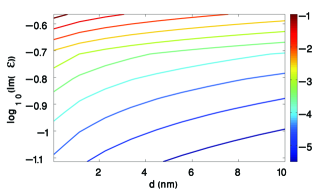
Figure 3: (Color online) Contour plot of $log_{10}X^{*}$as a function of $Im(\varepsilon)$ and $d=0nm$.

According to Fig.3, the heat flux reaches to 0.1 when imaginary part of dielectric constant is at range $0.20<Im(\varepsilon)\leq 0.27$ and $0\leq d\leq 7nm$. In comparison with Fig.2, the heat flux increases by one order of magnitude. It means that the heat flux is amplified by choosing the $G/SiO_{2}$ structure.By using the value of $Im(\varepsilon)$ and Eq.28 we find $1.006<v=\omega/E_{F}\leq 1.012$. On the Plasmon mode dispersion curve, the point $(q/k_{F},\omega/E_{F})=(1,1.01)$ is placed on the boundaries of the single particle excitation (SPE) for intra- and inter-band electron excitation in graphene Hwang and Sarma (2007); Jablan et al. (2009). Thus, the heat flux has a maximum at Plasmon frequency supported by the $G/SiO_{2}$ slabs.

Now let us to add the SG layer between two $G/SiO_{2}$ layers as Fig.1 shows. The total heat flow on SG layer from left $G/SiO_{2}$ layer is proportional to $[n_{B}(E,T_{1})-n_{B}(E,T_{2})]$ and the total heat flow on right $G/SiO_{2}$ layer from SG layer is equal to $[n_{B}(E,T_{2})-n_{B}(E,T_{3})]$. We choose the temperature $T_{2}$ the value such that the total heat flux on SG layer is zero i.e.,

$$n_{B}(E,T_{1})-n_{B}(E,T_{2})=n_{B}(E,T_{2})-n_{B}(E,T_{3})$$ (36)

or

$$T_{2}={\frac{1}{k_{B}\hbar\omega}}Ln[1+{\frac{2(e^{\beta_{1}\hbar\omega}-1)(e^{\beta_{3}\hbar\omega}-1)}{(e^{\beta_{1}\hbar\omega}-1)+(e^{\beta_{3}\hbar\omega}-1)}}]$$ (37)

Here, we assume $T_{1}=300K$, $T_{3}=323K$. Fig.4 (a) shows the heat flux $log_{10}{[n_{B}(E,T_{i})-n_{B}(E,T_{j})]X^{*}}$ between right (left) $G/SiO_{2}$ layer and SG layer and Fig.4 (b) shows the heat flux between two $G/SiO_{2}$ layers.

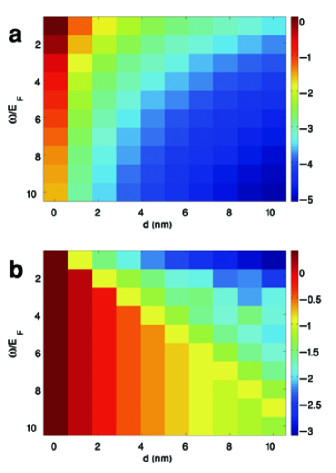
Figure 4: (Color online) (a) Heat flux between $G/SiO_{2}$ layer and SG layer and (b) between two $G/SiO_{2}$ layers. Here, colorbar shows $log_{10}{[n_{B}(E,T_{i})-n_{B}(E,T_{j})]X^{*}}$ .

The heat flow between $G/SiO_{2}$ and SG layer is maximized for $d\rightarrow 0$ and $\omega/E_{F}\rightarrow 1$. Therefore, it is maximized at Plasmon frequency which is placed on the boundaries of the SPE for intra- and inter-band electron excitation (note, $x={q}/{k_{F}}=1$). As Fig.4 (b) shows, for $1\leq{\omega}/{E_{F}}\leq 10$ and $d\leq 1nm$, then $[n_{B}(E,T_{i})-n_{B}(E,T_{j})]X^{*}\rightarrow 0.5$. Also for $2\leq{\omega}/{E_{F}}\leq 10$ and $d\leq 3nm$, then $-0.5<[n_{B}(E,T_{i})-n_{B}(E,T_{j})]X^{*}<0.5$. It means that for a wide range of Plasmon frequency and gap thickness the heat flux has maximum. Finally, as Fig.5 shows, the ratio of heat flux after adding the SG layer to before adding the layer depends on $\omega/E_{F}$ and $d$ but the heat flux is only amplified for specific range of $\omega/E_{F}$ and $d$ by adding the intermediate SG layer.

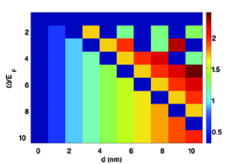
Figure 5: (Color online) The ratio of heat flux after adding the SG layer to before adding the layer.

It can be understood by looking at the coupling of modes between each $G/SiO_{2}$ layer and middle SG layer Messina et al. (2012). i.e., since the total heat transmission between two $G/SiO_{2}$ layers $\Phi_{13}$ is proportional to:

$$\Phi_{13}\propto[n_{B}(E,T_{1})-n_{B}(E,T_{2})]X^{*}+[n_{B}(E,T_{2})-n_{B}(E,T_{3})]X^{*}$$ (38)

and $n_{B,12}=n_{B,23}=n_{B,13}/2$, therefore $\tau_{13}=(\tau_{12}+\tau_{23})/2$ where $\tau_{ij}$ is the transmission probability between layer $i$ and layer $j$ Messina et al. (2012).

IV Summary

We have considered a suspended graphene (SG) layer between two Graphene on $SiO_{2}$ layers $(G/SiO_{2})$ and studied the heat flux amplification between two $G/SiO_{2}$ layers. It has been shown that, before adding the SG layer, the heat flux had maximum at Plasmon frequency supported by the $G/SiO_{2}$ slabs. By adding the SG layer, the heat flux between two $G/SiO_{2}$ was amplified, for specific range of vacuum gap between SG layer and $G/SiO_{2}$ layers and Plasmon freqency, due to the modes coupling between each $G/SiO_{2}$ layer and middle SG layer. Since the intermediate SG layer was a single atmoic layer, the heat transfer did not depend on the thickness of middle layer.

References

- Landau and Lifshitz (1960) L. . Landau and E. M. Lifshitz, Electrodynamics of Continuous Media (Pergamon, New York, 1960).
- Lifshitz (1955) E. M. Lifshitz, Zh. Eksp. Teor. Fiz. 29, 94 (1955).
- London (1930) F. London, Z. Phys. 63, 245 (1930).
- Abrikosova and Derjaguin (1953) I. I. Abrikosova and B. V. Derjaguin, Dok. Akad. Nauk SSSR 90, 1055 (1953).
- Loomis and Maris (1994) J. J. Loomis and H. J. Maris, Phys Rev. B 50, 24 (1994).
- Sipe (1987) J. E. Sipe, J. Opt. Soc. Am. 4, 4 (1987).
- Narayanaswamy and Chen (2010) A. Narayanaswamy and G. Chen, Quant. Spec. Radia. Tran. 111, 1877 (2010).
- Narayanaswamy and Zheng (2014) A. Narayanaswamy and Y. Zheng, Quant. Spec. Radia. Tran. 132, 12 (2014).
- Polder and Vanhove (1971) D. Polder and M. Vanhove, Phys Rev. B 4, 3303 (1971).
- Mulet et al. (2002) J. P. Mulet, K. Joulain, R. Carminati, and J. J. Greffet, Microscale Thermophys Eng. 6, 209 (2002).
- Fu and Zhang (2006) C. J. Fu and Z. M. Zhang, Int. J. Heat Mass Transfer 49, 1703 (2006).
- Chapuis et al. (2008) P. O. Chapuis, S. Volz, C. Henkel, K. Joulain, and J. J. Greffet, Phys. Rev. B 77, 035431 (2008).
- Volokitin and Persson (2001) A. I. Volokitin and B. N. J. Persson, Phys Rev. B 63, 205404 (2001).
- Basu and Zhang (2009) S. Basu and Z. M. Zhang, J. Appl. Phys 105, 093535 (2009).
- Joulain et al. (2005) K. Joulain, J. P. Mulet, F. Marquier, R. Carminati, and J. J. Greffet, Surf. Sci. Rep. 57, 59 (2005).
- Volokitin and Persson (2007) A. I. Volokitin and B. N. J. Persson, Rev. Mod. Phys 79, 1291 (2007).
- Kittle et al. (2005) A. Kittle, W. Muller-Hirsch, J. Parisi, S. A. Biehs, D. Redding, and M. Holthaus, Phys Rev Lett. 95, 224301 (2005).
- Hu et al. (2008) L. Hu, A. Narayanaswamy, X. Chen, and G. Chen, Appl. Phys. Lett. 92, 133106 (2008).
- Rousseau et al. (2009) E. Rousseau, A. Siria, G. Joourdan, S. Volz, F. Comin, J. Chevrier, and J. J. Greffet, Nature Photon 3, 514 (2009).
- Shen et al. (2009) S. Shen, A. Narayanaswamy, and G. Chen, Nano Lett. 9, 2909 (2009).
- Kralik et al. (2011) T. Kralik, P. Hanzelka, V. Musilova, A. Srnka, and M. Zobac, Rev. Sci. Instrum. 82, 055106 (2011).
- Ottens et al. (2011) R. S. Ottens, V. Quetschke, S. Wise, A. A. Alemi, R. Lundock, G. Mueller, D. H. Reitze, D. B. Tanner, and B. Whiting, Phys. Rev. Lett. 107, 014301 (2011).
- Messina et al. (2012) R. Messina, M. Antezza, and P. Ben-Abdallah, (2012), qunt-ph/1205.2076v1 .
- DiMatteo et al. (2001) R. S. DiMatteo, P. Greiff, S. L. Finberg, K. A. Young-Waithe, H. K. H. Choy, M. M. Masaki, and C. G. Fonstad, Appl. Phys. Lett. 79, 1894 (2001).
- Narayanaswamy and Chen (2003) A. Narayanaswamy and G. Chen, Appl. Phys. Lett. 82, 3544 (2003).
- Srituravanich et al. (2004) W. Srituravanich, N. Fang, C. Sun, Q. Luo, and X. Zhang, Nano Lett. 4, 1085 (2004).
- Wilde et al. (2006) Y. D. Wilde, F. Formanek, R. Carminati, B. Gralak, P. A. Lemoine, K. Goulain, J. P. Mulet, Y. Chen, and J. J. Greffet, Nature 444, 740 (2006).
- Jones and Raschke (2012) A. C. Jones and M. B. Raschke, Nano Letters 12, 1475 (2012).
- Nagaosa (1999) N. Nagaosa, Quantum Field Theory in Condensed Matter Physics (Springer, 1999).
- Scholz (2013) A. Scholz, Charge and current response of spin-orbit coupled two-dimensional materials (PhD Thesis, University of Regensburg, which can be downloaded on internet, 2013).
- Hwang and Sarma (2007) E. H. Hwang and S. D. Sarma, (2007), cond-mat/0610561v3 .
- Jablan et al. (2009) M. Jablan, H. Buljan, and M. Soljacic, Phys Rev B 80, 245435 (2009).