Limits of applicability of the quasilinear approximation to the electrostatic wave-plasma interaction

Abstract

The limitation of the Quasilinear Theory (QLT) to describe the diffusion of electrons and ions in velocity space when interacting with a spectrum of large amplitude electrostatic Langmuir, Upper and Lower hybrid waves, is analyzed. We analytically and numerically estimate the threshold for the amplitude of the waves above which the QLT breaks down, using a test particle code. The evolution of the velocity distribution, the velocity-space diffusion coefficients, the driven current, and the heating of the particles are investigated, for the interaction with small and large amplitude electrostatic waves, i.e. in both regimes, there where QLT is valid and there where it clearly breaks down.

I Introduction

The theory that describes the interaction between charged particles with a spectrum of low-amplitude waves in plasmas, is termed quasilinear theory (QLT) and has been widely studied and used in many applications. The theory for non-relativistic particles has been analyzed by Kennel and Englemann (1966), and the one for relativistic particles by Lerche (1968).

Tao et al. (2011) tested the theory of Kennel and Englemann (1966) for parallel propagation of Whistler modes, using a relativistic particle code, and found perfect agreement between the theoretical and their numerical diffusion coefficients for low-amplitude modes, i.e. in the quasilinear regime, thus validating the theory.

Although QLT is really practical and relatively simple, its downside lies in its limited applicability. The linearization approach that QLT adopts can be applied only in low-amplitude turbulence, where nonlinear wave-particle interactions and nonlinear wave-wave couplings are negligible.

QLT can also be applied when a single wave is assumed. The stochastic heating of ions by a single lower hybrid wave, propagating almost purely perpendicularly to a uniform magnetic field, was studied by Karney (1979), and the diffusion coefficients in velocity space were derived. Karney (1978) proved that if the wave amplitude remains below a certain threshold, the diffusion coefficient is similar to the one estimated by Kennel and Englemann (1966) and the damping of the wave is linear. Above this threshold though, and for finite wave amplitudes where nonlinear effects appear, stochasticity governs the phase-space, the resonances are broadened, and the ions get directly heated by the wave, irrespective of how close the frequency of the wave is to a cyclotron harmonic (i.e. the resonance condition is not a necessary condition for efficient particle heating). Detailed discussion on the nature and physical interpretation of this behavior can be found in several articles Smith and Kaufman (1978); Gell and Nakach (1980); Shklyar (1986). Benkadda, Sen, and Shklyar (1996) studied the role of an additional, second, obliquely propagating wave and found that the particle motion in such cases is much more complicated, and that the stochasticity threshold for the first wave’s amplitude is reduced due to nonlinear modification of the cyclotron resonances, caused by the presence of the second wave.

The investigation of the validity of QLT for a continuous spectrum of waves is a subject of interest as well, since it is a more realistic case. Lange et al. (2013) showed that for steep spectra, QLT is not able to predict a resonance (this point was also discussed by Shalchi et al. (2004)), since it manifests an irregularity around the resonant point. This is a known problem with QLTLange and Spanier (2012).

Our analysis in this article is based on resonant wave-particle interactions that lead to acceleration and heating of the particles in the presence of electrostatic waves (Langmuir waves (LW), Upper Hybrid (UH), and Lower Hybrid (LH) waves). We focus on the theoretical description of the case of non-relativistic particles, and by using the test particle approach we estimate the validity of QLT by comparing the analytical and numerical diffusion coefficients and velocity distribution functions of the particles. We begin by setting the wave amplitude low enough for QLT to be valid, and then gradually increase the amplitudes of the waves and monitor the departure from the predictions of the QLT. We start our analysis with the case of LW, which have extensively been discussed in the literature Sagdeev and Galeev (1969), and we use this study as a basis to test our numerical model and then expand our study to the cases of UH and LH waves.

This paper is structured as follows. In Section II a brief general description of our model is presented. Sections III and IV summarize the analytical and numerical results for the cases of Langmuir, UH, and LH waves, respectively. We then discuss the results in Section V. Additionally, Appendix A gives some details on the derivation of the UH and LH dispersion relations, and Appendix B includes some calculations required for deriving the diffusion coefficients in these two cases.

II Model description

II.1 Initial Settings

We consider a non-relativistic and collisionless plasma of temperature $T$ and number density $n_{0}$, with total plasma thermal energy $\mathcal{W}_{tot}$, with the plasma being either magnetized or unmagnetized. The electric field $\mathbf{E}(\mathbf{x},t)$ is considered to be a superposition of many electrostatic modes $\delta\mathbf{E}_{\mathbf{k}}(\mathbf{x},t)$, each having a random phase $\vartheta_{\mathbf{k}}$ and energy density Nicholson (1983); Sagdeev and Galeev (1969); Frisch (1995)

$$\mathcal{W}_{\mathbf{k}}(t)\equiv\frac{|\delta\mathbf{E}_{\mathbf{k}}|^{2}}{8\pi}=ak^{-5/3},$$ (1)

i.e. we assume that the wave energy density spectrum follows a Kolmogorov power-law. The normalization constant, $a$, is such that it satisfies the condition

$$W_{0}=\int_{k_{\min}}^{k_{\max}}\mathcal{W}_{\mathbf{k}}(t=0)dk\equiv\kappa W_{\rm tot}$$ (2)

at initial time $t=0$, where $W_{0}$ is the total wave energy density, which is taken to be a fraction $\kappa$ of $W_{\rm tot}$, and $k_{min},k_{max}$ are the limits of the wave spectrum. The coefficient $\kappa$ is a free parameter in our analysis.

We assume that the particles have initially a velocity distribution function which is of the form of an isotropic Maxwellian,

$$f^{s}(\mathbf{v},t=0)\equiv\frac{n_{0}}{\left(\sqrt{2\pi}\;u_{\rm th,s}\right)^{3}}\exp\left(-\frac{\mathbf{v}^{2}}{2u_{\rm th,s}^{2}}\right)$$ (3)

where $u_{\rm th,s}\equiv(T_{s}/m_{s})^{1/2}$ is their thermal speed, and $s=e/i$ denotes electrons/ions.

The wave-particle interaction modifies the initial velocity distribution by absorbing energy from the waves. The QLT is built on the assumption that we can split the distribution function into two parts, namely the averaged slowly varying part, $f^{s}_{0}(\mathbf{v},t)\equiv\langle f^{s}(\mathbf{x},\mathbf{v},t)\rangle_{\mathbf{x}}$, and the first order rapidly varying perturbation, $\delta f^{s}(\mathbf{x},\mathbf{v},t)\equiv f^{s}(\mathbf{x},\mathbf{v},t)-\langle f^{s}(\mathbf{x},\mathbf{v},t)\rangle_{\mathbf{x}}$. In this context then, one can derive the diffusion equation for $f^{s}_{0}$ by solving the set of equations consisting of the averaged and linearized Vlasov equations, combined with the Maxwell equations. This diffusion equation can be written as

$$\frac{\partial f^{s}_{0}(\mathbf{v},t)}{\partial t}=\nabla_{\mathbf{v}}\cdot\left[D_{s}^{\rm QL}(\mathbf{v},t)\nabla_{\mathbf{v}}f^{s}_{0}(\mathbf{v},t)\right]$$ (4)

with the velocity diffusion tensor Kennel and Englemann (1966)

$$D_{s}^{\rm QL}(\mathbf{v},t)\equiv i\frac{e^{2}}{m_{s}^{2}}\int d^{3}\mathbf{k}\sum\limits_{n=-\infty}^{\infty}\frac{\left(\mathbf{d}^{s}_{n,\mathbf{k}}\right)^{*}\mathbf{d}^{s}_{n,\mathbf{k}}}{\sigma_{\mathbf{k}}-k_{\|}v_{\|}-n\Omega_{s}},$$ (5)

where the vector

$$\mathbf{d}^{s}_{n,\mathbf{k}}\equiv\mathcal{E}^{s}_{n,\mathbf{k}} \left[\mathbf{\hat{e}}_{\perp}\left(1-\frac{k_{\|}v_{\|}}{\sigma_{\mathbf{k}}}\right)+\hat{\mathbf{e}}_{\|}\frac{k_{\|}v_{\perp}}{\sigma_{\mathbf{k}}}\right]+\left(E_{\|}\right)_{\mathbf{k}}J_{n}(\zeta_{\mathbf{k}}^{s})$$ (6)

$$\times\left[\mathbf{\hat{e}}_{\|}\left(1-\frac{n\Omega_{s}}{\sigma_{\mathbf{k}}}\right)+\mathbf{\hat{e}}_{\perp}\frac{n\Omega_{s}}{\sigma_{\mathbf{k}}}\frac{v_{\|}}{v_{\perp}}\right],$$

with $\mathbf{\hat{e}}_{\perp}\equiv\mathbf{v}_{\perp}/|\mathbf{v}_{\perp}|$ and $\mathbf{\hat{e}}_{\|}\equiv\mathbf{\hat{e}}_{\mathbf{z}}$, by assuming that the magnetic field points along the $z$-direction, and where $\sigma_{\mathbf{k}}=\omega_{\mathbf{k}}+i\gamma_{\mathbf{k}}$ is the complex frequency of the waves. Here, $J_{n}(\zeta_{\mathbf{k}}^{s})$ are the Bessel functions of first kind, where $\zeta_{\mathbf{k}}^{s}\equiv k_{\perp}v_{\perp}/\Omega_{s}$, $\Omega_{s}$ is the gyrofrequency and the symbols $\|$ and $\perp$ denote the direction parallel and perpendicular to the magnetic field, respectively. Finally, also the definition

$$\mathcal{E}^{s}_{n,\mathbf{k}} \equiv \frac{E_{x}(\mathbf{k})}{2}\left[e^{i\psi}J_{n+1}(\zeta_{\mathbf{k}}^{s})+e^{-i\psi}J_{n-1}(\zeta_{\mathbf{k}}^{s})\right]$$ (7)

$$+i\frac{E_{y}(\mathbf{k})}{2}\left[e^{i\psi}J_{n+1}(\zeta_{\mathbf{k}}^{s})-e^{-i\psi}J_{n-1}(\zeta_{\mathbf{k}}^{s})\right]$$

is used, where $\psi$ is the polar angle of $\mathbf{k}_{\perp}$.

In order to derive the diffusion rates for specific kinds of waves, we must couple Eq. (4) with the linearized Poisson equation,

$$i\;\mathbf{k}\cdot\delta\mathbf{E}_{\mathbf{k}}(t)=4\pi e\int d^{3}\mathbf{v}\;\left[\delta f^{i}_{\mathbf{k}}(\mathbf{v},t)-\delta f^{e}_{\mathbf{k}}(\mathbf{v},t)\right],$$ (8)

from which the linear dispersion relation can be derived. The $\delta f^{s}_{\mathbf{k}}$ that is needed can be expressed as Kennel and Englemann (1966)

$$\delta f^{s}_{\mathbf{k}}=-i\frac{(\pm e)}{m_{s}}E_{\mathbf{k}}\sum\limits_{n,m=-\infty}^{\infty} \frac{nJ_{n}(\zeta_{\mathbf{k}}^{s})J_{m}(\zeta_{\mathbf{k}}^{s})}{\zeta_{\mathbf{k}}^{s}}$$ (9)

$$\times\frac{e^{i(m-n)(\phi-\psi)}}{\sigma_{\mathbf{k}}-n\Omega_{s}}\frac{\partial f^{s}_{0}}{\partial v_{\perp}},$$

and the derivation of the dispersion relation then is straightforward (as briefly presented in Appendix A).

The QLT describes the slowly varying distribution function $f_{0}^{s}$, and in order to be valid, it needs to be ensured that $f_{0}^{s}$ changes slowly enough, and more specifically its diffusive relaxation time, $\tau_{R}$ (defined below), must be clearly longer than the wave-particle interaction time-scale Chirikov (1979); Diamond, Itoh, and Itoh (2009); Shapiro and Sagdeev (1997) $|\gamma_{\mathbf{k}}|^{-1}$ (with $\gamma_{\mathbf{k}}$ the growth rate, see below), thus

$$\tau_{R}\gg|\gamma_{\mathbf{k}}|^{-1}.$$ (10)

If that is the case, the space-averaged distribution function changes slowly enough, so that particles, which gyrate around the magnetic field and diffuse in velocity-space, do not experience any changes of $f^{s}_{0}$ on their characteristic gyro-motion and wave-motion timescales.Kennel and Englemann (1966); Chew, Goldberger, and Low (1956) Then, any dependence of $f^{s}_{0}$ on the velocity polar angle, $\phi=\tan^{-1}\left(v_{y}/v_{x}\right)$, is weak and averages out over a complete rotation from $0$ to $2\pi$, and therefore the diffusion process becomes two-dimensionalKennel and Englemann (1966) in the ($v_{\perp},v_{\|}$)-space.

In all the three normal modes (LW, UH, LH) that we will study, we will derive the upper limit for the wave amplitude for the QLT’s applicability, using condition (10).

When this condition is not satisfied, the rapid energy exchange during the wave-particle interaction, and hence the rapid distribution function modification, does not allow the application of QLT’s equations in the form presented above. In addition, for QLT to be applicable in each of these cases, the Chirikov overlap criterion must be satisfied, so that the particles do not get trapped inside enhanced electric field structures, but travel relatively unhindered in velocity space. In more specific terms, this condition can be expressed Diamond, Itoh, and Itoh (2009) as $1/\tau_{b}<1/\tau_{ac}$, where $\tau_{b}$ is the bounce time-scale of the particles in the field, and $\tau_{ac}$ is the electric field’s autocorrelation time-scale.

II.2 Numerical model

In our numerical model, we use a large a number of test particles, initially randomly distributed in space inside a periodic and cubic box in the plasma, and obeying a Maxwellian distribution function (3) in velocity-space. The spectrum of waves used has $k\in[k_{\min},k_{\max}]$, and in total it initially carries the energy density $W_{0}$.

A test particle evolves according to the Lorentz force, $d\mathbf{p}/dt=\pm e\left(\mathbf{E}+\bm{\beta}\times\mathbf{B}\right)$, where $\bm{\beta}\equiv\mathbf{v}/c$, $\mathbf{v}$ is the velocity and $\mathbf{p}$ the momentum. With $\mathbf{p}=\gamma m_{s}\mathbf{v}$, where the relativistic factor is $\gamma\equiv\left(1-\bm{\beta}^{2}\right)^{-1/2}$, we can write the equations of motion in the following form,

$$\frac{d\bm{\beta}}{dt}=\mp\frac{e}{c\gamma m_{s}}(\bm{\beta}\cdot\mathbf{E})\bm{\beta}\pm\frac{e}{c\gamma m_{s}}\mathbf{E}+\Omega_{s}\bm{\beta}\times\hat{\mathbf{e}}_{\|}$$ (11)

in which $\Omega_{s}$ is the relativistic gyrofrequency, and where we also used the relation $d(c^{2}\gamma m_{s})/dt=\pm e\mathbf{v}\cdot\mathbf{E}$.Bittencourt (2004).

Solving the equations of motion, the numerical diffusion coefficient is calculated according to

$$D\equiv\lim\limits_{\delta t\rightarrow 0}\frac{\langle\delta\mathbf{v}^{2}\rangle}{2\delta t},$$ (12)

in which the average is taken over the particles, divided into groups of similar initial velocities, and also $\delta\mathbf{v}=\mathbf{v}(t)-\mathbf{v}(t-\delta t)$, with relatively small values for $\delta t$, as indicated in the applications below Ragwitz and Kantz (2001).

In the simulations we consider times such that $|\gamma_{k}|t\ll 1$, during which the energy loss of the waves is transferred to the test particles. Specifically, in the case of Langmuir waves, $\gamma_{\mathbf{k}}\propto(\partial f/\partial v)_{v\simeq\omega_{e}/k}$, and the formation of a plateau in the resonant region $v\simeq\omega_{k}/k$ quickly leads $\gamma_{k}$ to vanish. In the case of UH waves, the magnetic field is taken to be strong so $|\gamma_{k}|$ is small compared to $|\Omega_{e}|$, and remains unchanged for the resonance condition $\omega_{k}\simeq|\Omega_{e}|$. The same is true in the case of LH waves, but here the resonance condition is $\omega_{\mathbf{k}}\simeq\Omega_{i}$ (see Section IV, and Appendix A). Therefore, $\mathcal{W}_{k}(t)=\mathcal{W}_{k}(0)\exp(2\gamma_{k}t)\simeq\mathcal{W}_{k}(0)(1+2\gamma_{k}t)\simeq\mathcal{W}_{\mathbf{k}}(0)$, hence the wave energy changes only slightly during our simulations.

III Langmuir Waves

In this section we perform a first check of the QLT prediction about the maximum wave energy limit beyond which it stops being valid for the LW. The theory is presented briefly, since it is extensively analyzed in the literature (see for example Sagdeev and Galeev (1969)), and it is then tested using the analytical formulas and the numerical estimates.

III.1 Analytical predictions

In the absence of a magnetic field, $\Omega_{e}=0$, we can select $\hat{e}_{\mathbf{z}}$ as the propagation direction for the waves. Then, for $\mathbf{E}_{\mathbf{k}}=E_{\mathbf{k}}\mathbf{\hat{e}}_{\mathbf{z}}$, from Eq. (7) it is easy to show that $\mathcal{E}_{n,\mathbf{k}}=0$. Taking first the purely parallel propagation limit, $k_{\perp}\rightarrow 0^{+}$ and then the zero-magnetic field limit, $\Omega_{e}\rightarrow 0^{-}$, the Bessel function in $\mathbf{d}_{n,\mathbf{k}}$ is replaced by unity for $n=0$ in the sum of Eq. (5), since $J_{n}(0)=\delta_{n0}$. Thus, the diffusion tensor in Eq. (5) has only one non-zero component, the $\mathbf{\hat{e}}_{\mathbf{z}}\mathbf{\hat{e}}_{\mathbf{z}}$ term, which is simplified to

$$D^{\rm QL}(v)=8\pi^{2}\left(\frac{e}{m_{e}}\right)^{2}\int d^{3}\mathbf{k}\left[\mathcal{P}\frac{\gamma_{\mathbf{k}}\mathcal{W}_{\mathbf{k}}}{\left(\omega_{\mathbf{k}}-kv\right)^{2}+\gamma_{k}^{2}}+\pi\mathcal{W}_{\mathbf{k}}\delta\left(\omega_{\mathbf{k}}-kv\right)\right],$$ (13)

after dropping every unnecessary index, since the diffusion is one-dimensional and only electrons are considered, and where the symbol $\mathcal{P}$ denotes principal value. The imaginary part of this sum does not contribute, since it vanishes in the summation. Eq. (13) is the already known Sagdeev and Galeev (1969) diffusion coefficient for Langmuir oscillations which takes into consideration the resonant particles through the delta function selection rule, as well as the non-resonant particles, which form the bulk distribution, through the integral over the principal value. Resonances involve particles with velocities $v\simeq\omega_{\mathbf{k}}/k$, which resonate with the corresponding waves.

Solving the linearized Vlasov equation for $\delta f_{\mathbf{k}}$ and substituting the solution into Eq. (8) (in which only the electrons will appear due to the high frequency of the oscillations), it can be shown that the real part of the resulting equation has the solution $\omega_{\mathbf{k}}^{2}=\omega_{e}^{2}\left[1+(3/2)\left(k\lambda_{e}\right)^{2}\right]$, where $\lambda_{e}$ is the electron Debye length, and which is expected since it expresses the Langmuir wave dispersion relation. Concerning the imaginary part $\gamma_{\mathbf{k}}$ of the frequency, we assume that $|\gamma_{\mathbf{k}}|\ll\omega_{\mathbf{k}}$, and from the resulting imaginary part of Eq. (8), combined with the previous solution for $\omega_{\mathbf{k}}$, we get the solution for $\gamma_{\mathbf{k}}$, which is

$$\gamma_{\mathbf{k}}\simeq\frac{\pi}{2}\frac{\omega_{\mathbf{k}}\omega_{e}^{2}}{n_{0}k^{2}}\left(\frac{\partial f_{0}}{\partial v}\right)_{v\simeq\omega_{\mathbf{k}}/k}.$$ (14)

For a Maxwellian initial distribution, $f_{0}$, the damping coefficient is $\gamma_{\mathbf{k}}\propto-\exp\left[-2^{-1}\left(k\lambda_{e}\right)^{-2}(\omega_{\mathbf{k}}/\omega_{e})^{2}\right]$, so the damping is weak if $k\lambda_{e}\ll 1$, in which case the expressions for the two frequency parts simplify to $\omega_{\mathbf{k}}\simeq\omega_{e}$ and $\gamma_{\mathbf{k}}\simeq(\pi/2)(\omega_{e}^{3}/n_{0}k^{2})(\partial f_{0}/\partial v)_{v\simeq\omega_{\mathbf{k}}/k}$.

In the steady state limit, $\partial f(v,t\rightarrow\infty)/\partial t=0$, and in the resonance region the diffusion equation, Eq. (4), implies that

$$\left.\left\{\left[\frac{\mathcal{W}_{\mathbf{k}}(t\rightarrow\infty)}{v}\right]\frac{\partial f_{0}(v,t\rightarrow\infty)}{\partial v}\right\}\right|_{v\simeq\omega_{\mathbf{k}}/k}=0$$ (15)

will hold. If we assume that the waves initially contain enough energy to fuel the whole energy exchange process (which is true in our case), then the only possible result of Eq. (15) is the modification of the resonant distribution part, $f_{0}^{\rm r}$, as $[\partial f_{0}^{\rm r}(v,t\rightarrow\infty)/\partial v]_{v\simeq\omega_{\mathbf{k}}/k}=0$, i.e. a plateau will be formed and the resonant part of the distribution stops evolving. The plateau can easily be calculated as the mean value of $f_{0}$ in the resonant region in the time-asymptotic limit, and it isSagdeev and Galeev (1969)

$$\bar{f}_{0}^{\rm r}(t\rightarrow\infty)=\frac{1}{v_{\max}-v_{\min}}\int_{v_{\min}}^{v_{\max}}f(v,t\rightarrow\infty)dv,$$ (16)

where $\bar{f}_{0}^{r}(t\rightarrow\infty)$ is the value of the distribution at the plateau. The non-resonant distribution part, $f_{0}^{\rm nr}$, on the other hand, remains relatively unchanged, with a small increase in temperatureSagdeev and Galeev (1969).

For a wave-spectrum of width $\Delta(\omega_{\mathbf{k}}/k)$, we can derive an approximate expression for the relaxation time $\tau_{R}=[\Delta(\omega_{\mathbf{k}}/k)]^{2}/D^{\rm QL}$ of the particle diffusion as

$$\tau_{R}\simeq\frac{n_{0}m_{e}k\left[\Delta(\omega_{e}/k)\right]^{3}}{2\pi\omega_{e}^{2}W_{0}}.$$ (17)

It then follows that in order for condition (10) to hold, $\kappa$ must be in the range indicated by

$$\kappa\ll\kappa_{\rm LM}^{\rm QL}\equiv\frac{n_{0}m_{e}\omega_{e}^{2}\left[\Delta(\omega_{e}/k)\right]^{3}}{4\sqrt{2\pi}k^{2}u_{\rm th,e}^{3}W_{\rm tot}}\exp\left[-\frac{1}{2}\left(\frac{\omega_{e}}{ku_{\rm th,e}}\right)^{2}\right]$$ (18)

(as an order of magnitude approximation), where the notation $\kappa_{\rm LM}^{\rm QL}$ is used to denote the upper limit of the range of $\kappa$ values for which QLT is valid, according to the analytical results. For a more accurate approximation of the upper limit for QLT’s validity, we need to study the problem numerically.

III.2 Numerical results

The parameters used for our numerical calculations are the total number of test-particles $N_{p}=2\times 10^{4}$, the density $n_{0}(cm^{-3})=10^{9},$ the temperature $T(eV)=100$, and the wave phase velocity range $v_{min}/u_{th}=2,u_{max}/u_{th}=4$. The initial velocity distribution of the test particles is a Maxwellian, as in Eq. (3), and in space the particles are randomly distributed in a box of linear size $2\cdot 10^{5}\lambda_{e}$. We consider a spectrum of $100$ waves, each assumed to have a random phase in $[0,2\pi]$, and their amplitudes follow the power-law of Eq. (1).

[] [] [] [] [] []

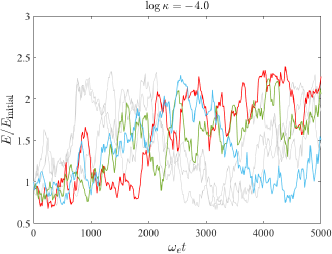
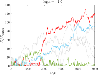
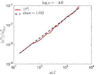
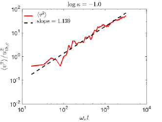
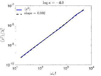
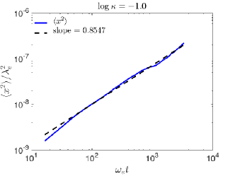
Figure 1: The evolution over time of the energy of six randomly selected particles, normalized by their initial energy (LABEL:sub@fig:langmuir_energies_-4 and LABEL:sub@fig:langmuir_energies_-1), the mean square displacement in velocity space (LABEL:sub@fig:vMSD_-4 and LABEL:sub@fig:vMSD_-1), and the mean square displacement in position space (LABEL:sub@fig:xMSD_-4 and LABEL:sub@fig:xMSD_-1), for $\kappa=10^{-4}$, where QLT is expected to work (left column), and for $\kappa=10^{-1}$, where QLT is expected to be invalid (right column).

FIG. 1 shows the evolution of the energy of six, out of in total $N_{p}$, randomly selected particles. For the case in FIG. 1 that the waves carry energy equal to $0.01$% of the total plasma thermal energy, the energy of the particles evolves in a stochastic, random walk like manner. If the wave energy increases to $10$% of the total plasma thermal energy, as in FIG. 1, the evolution still is random walk like, the particles though experience abrupt energy jumps over short times, in some cases $2-3$ orders of magnitude larger than their initial energy, Also note the much more extended dynamical range in FIG. 1 compared to FIG. 1. The random walk character of the evolution is visible on time-scales large enough so that the particles have entered the diffusive regime, and we find that the time needed for the particles to travel several tens of a typical wavelength is several hundreds of the plasma period. The diffusive time scale is also illustrated by the mean square displacements (MSD) in velocity and in position space, as also shown in FIG. 1. In the case of low energy waves, the MSD in velocity and position space is proportional to time, which implies that the diffusion is normal in both spaces and the random walk is of classical nature (FIGS. 1 and 1), whereas for the waves with larger energy content the diffusion process has become anomalous, namely super-diffusive in velocity space (FIG. 1) and sub-diffusive in position space (FIG. 1), which can clearly be attributed to nonlinear effects.

[] []

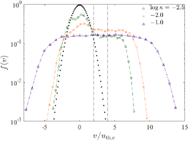
Figure 2: LABEL:sub@fig:langmuir_diffusion_coefficients For values of $\kappa<10^{-3.5}$, the numerical results are consistent with QLT, since the plateau (black solid line) is predicted by Eq. (16) accurately. LABEL:sub@fig:langmuir_current The initial distribution (black dotted line), for cases of $\kappa>10^{-3.5}$, is modified beyond QLT’s predictions. The vertical black dashed lines mark the minimum and maximum phase velocities of the excited waves.

The evolution of the particle velocity distribution function due to wave-particle interactions, for various values of $\kappa$, is shown in FIG. 2. According to Eq. (15), we expect that the initial Maxwellian velocity distribution will evolve to form a plateau inside the resonance region, while practically no change will be observed in the non-resonant part of it, provided that the wave energy is restricted by $\log\kappa\ll-2.3=\log\kappa_{\rm LM}^{\rm QL}$, according to condition (18). As seen in FIG. 2, for the range of wave energies with $\log\kappa<-3.5$ the velocity distribution’s evolution is predicted accurately by QLT. Above this threshold the plateau is broadened and the non-resonant part of the distribution is also modified, as FIG. 2 demonstrates, in which cases of waves carrying energy up to $10$% of the total plasma thermal energy are shown. The distribution in these cases is strongly modified and QLT fails to describe this modification.

[] []

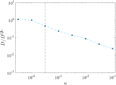
Figure 3: LABEL:sub@fig:langmuir_diffusion_coefficients Resonant test particle velocity diffusion coefficients according to Eq. (12), with $\delta t\simeq 30\omega_{e}^{-1}$, normalized by the analytical expectation of the QLT. LABEL:sub@fig:langmuir_current Total electric current $J$ in the plasma, induced by the wave-particle interaction, in units of $-eu_{\rm th,e}$.

FIG. 3 shows the comparison between the theoretical prediction of the velocity diffusion coefficients for resonant particles and the diffusivities that were obtained numerically. For the cases of waves with $\log\kappa<-3.5$ the diffusion coefficients are in good agreement, thus QLT provides accurate results. For $\log\kappa\gtrsim-3.5$ an increasing disagreement starts to appear, and the QLT overestimates the diffusion rates in the resonant velocity range. In these cases, the wave amplitudes are too high to satisfy QLT’s prerequisites, the interaction is fully nonlinear and stochasticity comes into play in the non-resonant part of the phase space, so particles from the bulk of the velocity distribution diffuse very efficiently to very high velocities. This also leads to the flattening of the velocity distribution well outside the resonant part, which is very obvious in FIG. 2.

In FIG. 3 the total electric current, $J$, as induced by the wave-particle interaction, which breaks the isotropy of the initial Maxwellian, is shown as a function of $\kappa$. $J$ increases with increasing $\kappa$, until it starts to saturate above $\log\kappa\sim-2$. From then on, electrons with negative velocities are also noticeably accelerated, as can also be seen in Fig 2, hence the saturation of $J$.

Overall, we find that if $\log\kappa\lesssim-4$, QLT can be safely used as a valid description. The breaking point of the theory appears to be in the range of $\log\kappa\in[-4,-3.5]$, thus it is clearly $1.5$ orders of magnitude lower than the theoretical limit $\kappa_{\rm LM}^{\rm QL}$ in Eq. (18).

IV Upper Hybrid and Lower Hybrid waves

Now we study the quasilinear theory’s applicability for the case of purely perpendicularly propagating UH and LH waves. In this case, the turbulence is also electrostatic, and the resonances occur only in the perpendicular plane. These resonances result in the heating of the particles in $v_{\perp}$, while in $v_{\|}$ no significant energy gain is observed.

IV.1 Analytic predictions

As shown in Appendix A, by making some assumptions, one can express the dispersion relations as $\omega_{\mathbf{k}}\simeq|\Omega_{s}|$, and $\gamma_{\mathbf{k}}\simeq-(\pi/4)(\omega_{s}^{4}/|\Omega_{s}|^{3})$, where $s=e/i$ for UH/LH waves. Specifically, we have assumed small enough wave-numbers, and a strong magnetic field. Using the simplified expressions, it is easy to derive some important analytical results about the wave-particle interactions.

Table 1: Simulation parameters for the case of Upper Hybrid and Lower Hybrid waves.

Upper Hybrid		Lower Hybrid
Parameter	Value	Parameter	Value
$N_{p}$	$2\times 10^{4}$	$N_{p}$	$2\times 10^{4}$
$N_{k}$	$100$	$N_{k}$	$100$
$n_{0}({\rm cm}^{-3})$	$10^{9}$	$n_{0}({\rm cm}^{-3})$	$10^{9}$
$T({\rm eV})$	$100$	$T({\rm eV})$ a	$100$
$u_{\rm th,e}(c)$	$1.4\times 10^{-2}$	$u_{\rm th,i}(c)$	$3.3\times 10^{-4}$
$u_{\min}(u_{\rm th,e})$	$3.4$	$u_{\min}(u_{\rm th,i})$	$2.5$
$u_{\max}(u_{\rm th,e})$	$4.0$	$u_{\max}(u_{\rm th,i})$	$3.0$
$B_{0}({\rm G})$	$500$	$B_{0}({\rm kG})$	$7$

More specifically, since the turbulence is electrostatic, with $\mathbf{E}_{\mathbf{k}}=E_{\mathbf{k}}\mathbf{k}/k_{\perp}\equiv E_{\mathbf{k}}\mathbf{\hat{e}}_{\mathbf{x}}$, from Eq. (7) one concludes that $\mathcal{E}^{s}_{n,\mathbf{k}}=nE_{\mathbf{k}}J_{n}(\zeta^{s}_{\mathbf{k}})/\zeta^{s}_{\mathbf{k}}$, where $\zeta^{s}_{\mathbf{k}}\equiv k_{\perp}v_{\perp}/\Omega_{s}$, and hence from Eq. (6) it follows that the vector

$$\mathbf{d}^{s}_{n,\mathbf{k}}=\frac{nJ_{n}(\zeta^{s}_{\mathbf{k}})}{\zeta^{s}_{\mathbf{k}}}E_{\mathbf{k}}\mathbf{\hat{e}}_{\perp}.$$ (19)

Thus, Eq. (5) for the diffusion coefficients becomes

$$D^{\rm QL}_{\perp s}\simeq\frac{\pi\omega_{s}^{2}}{2n_{0}m_{s}|\Omega_{s}|}\int d^{3}\mathbf{k}\;\mathcal{W}_{\mathbf{k}},$$ (20)

as shown in Appendix B, and which is just the purely perpendicular component and the only non-zero part of Eq. (5). Resonances are purely in the perpendicular plane, and particles will be in gyro-resonance as long as the resonance condition $\omega_{\mathbf{k}}=n\Omega_{s}$ is satisfied, where $n$ is an integer. Also, we make sure that we select a strong enough magnetic field, such that the only resonance we observe is the $|n|=1$ in both cases.

Once again, the validity of quasilinear theory requires that the damping timescale $|\gamma_{\mathbf{k}}|^{-1}$ is much shorter than the averaged distribution’s relaxation time $\tau_{R}$, as expressed by the condition in Eq. (10), which here takes the form

$$\kappa\ll\kappa_{s}^{\rm QL}\equiv\frac{n_{0}m_{s}\omega_{s}^{2}\left[\Delta(|\Omega_{s}|/k_{\perp})\right]^{2}}{2\Omega_{s}^{2}W_{\rm tot}},$$ (21)

where $s=e$ corresponds to the UH case and we denote the upper limit for QLT’s validity according to the theory with $\kappa_{\rm UH}^{\rm QL}$, while the corresponding notation for the case of LH waves, with $s=i$, is $\kappa_{\rm LH}^{\rm QL}$. If this limit is satisfied, quasilinear theory is expected to be applicable, and the distribution function is expected to show heating. Also, in case of applicability, quasilinear theory can make an estimate of the temperature. Specifically, by applying the transformation $\partial t^{\prime}/\partial t=2D^{\rm QL}_{\perp s}$, we find as solution a Maxwellian with temperature

$$\Delta T_{s}^{\rm QL}\simeq\frac{\pi\omega_{s}^{2}W_{\rm tot}}{n_{0}|\Omega_{s}|}\kappa_{s}^{\rm QL}t,$$ (22)

and QLT is valid if $\Delta T_{s}^{\rm QL}/m_{s}\ll u_{\rm th,s}^{2}$.

IV.2 Numerical results

The parameters used in the simulations of the LH and UH wave cases are summarized in TABLE 1. The kinetic energies of individual test particles and the average energy behave in a similar fashion as in the LW case (see FIG. 1).

[] []

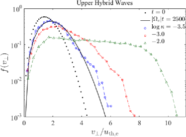
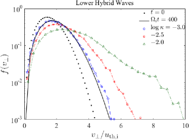
Figure 4: LABEL:sub@fig:upper_hybrid_distributions Evolution of the perpendicular electron velocity distribution function in the interaction with an excited spectrum of Upper Hybrid waves, for various $\kappa$ values. The final results correspond to $t=2500|\Omega_{e}|^{-1}$. LABEL:sub@fig:lower_hybrid_distributions Evolution of the perpendicular ion velocity distribution function in the interaction with an excited spectrum of Lower Hybrid waves, for various $\kappa$ values. The final results correspond to $t=400\Omega_{i}^{-1}$.

The analytical expectation for the upper limit of wave energy for QLT’s applicability in relation (21) suggests that it must hold that $\log\kappa\ll-2.8=\log\kappa_{\rm UH}^{\rm QL}$ for the case of UH waves, and $\log\kappa\ll-1.3=\log\kappa_{\rm LH}^{\rm QL}$ for the case of LH waves, by using the parameters in TABLE 1. If $\kappa$ is in the range suggested by these conditions, the velocity distribution function of the test particles is expected to show heating in the way predicted by Eq. (22), and the diffusion coefficients can be approximated by Eq. (20).

[] []

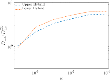
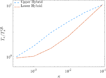
Figure 5: LABEL:sub@fig:hybrid_diffusion_coefficients Test electron and ion velocity diffusion coefficients, using the definition in Eq. (12), with $\delta t\simeq 200|\Omega_{e}|^{-1}$ and $\delta t\simeq 32\Omega_{i}^{-1}$ for the UH and LH waves, respectively, normalized by the analytically expected value, and for varying $\kappa$. LABEL:sub@fig:hybrid_temperatures Comparison between the temperature of the final distribution as predicted by Eq. (21) and the numerical results, for the cases of Upper Hybrid and Lower Hybrid waves, and for varying $\kappa$.

In FIG. 4, the evolution of the perpendicular electron velocity distribution function $f(v_{\perp})$ is shown for the case of UH waves. The heating of test-particles for $\log\kappa=-3.5$ is consistent with QLT’s prediction (Eq. (22)). If the wave energy is increased above this value, QLT underestimates the heating, and for $\log\kappa\geq-3$, the theory is not valid. Also, the results of the comparison between the numerical and analytical diffusion coefficients, shown in FIG. 5, confirm this limit, as $\kappa$ increases, an increasing disagreement between the numerical and theoretical results appears, and QLT underestimates the diffusion coefficients for $\kappa\gtrsim 10^{-3}$. Furthermore, in FIG. 5 the temperatures of the final distributions compared to Eq. (22) are shown. As can be seen, the results for the temperature indicate the same limit for $\kappa$, QLT underestimates the final temperature for $\kappa\gtrsim 10^{-3}$. Overall, the results suggest the wave energy range of $\log\kappa\lesssim-3.5$ for QLT’s applicability in the UH case, and that in the interval $\log\kappa\in[-3.5,-3]$ the first signs of QLT’s invalidity can be found. Thus, the maximum value of $\kappa$ for QLT’s validity is less than an order of magnitude lower than the theoretical $\kappa_{\rm UH}^{\rm QL}$.

The final perpendicular velocity distributions of the ions, after their interaction with an excited spectrum of LH waves, for various $\kappa$ values, is shown in FIG. 4. In this case, the theoretical heating (Eq. (22)) is consistent with the numerical results for $\log\kappa\lesssim-3$, and fails to describe the numerical results for larger values of the wave energy, by underestimating the final temperature. This also is obvious from FIG. 5, in which one can see that the analytical diffusion coefficients are systematically lower than the corresponding numerical ones if $\log\kappa>-3$. That there is also underestimation of the heating by QLT can be seen in FIG. 5, from which the same limit for $\kappa$ can be inferred. Thus, in the LH case, the upper limit for QLT’s validity can be estimated to lie in $\log\kappa\in[-3,-2.5]$, hence it is more than an order of magnitude lower than the theoretical $\kappa_{\rm LH}^{\rm QL}$.

V Summary

In this article, we explored the limitations of the QLT for the interaction of electrostatic waves (LW, UH, LH) with the plasma. We used a spectrum of waves with energy $W_{0}=\kappa W_{tot}$, where $W_{tot}$ is the total thermal energy of the plasma, and a test particle numerical code to analyze and search for the transition from the QLT to the non-linear evolution of the test-particles.

Our main results are the following:

1. For the LW case, using the basic criterion for the validity of the quasilinear approximation, i.e. the relaxation time of the particle evolution should be much shorter than the damping time of the waves, we estimated the maximum wave energy ($\kappa_{QL}$) below which the QLT is valid.

2. We estimated the diffusion coefficients analytically and numerically and demonstrated that when $\kappa>\kappa_{QL}$ then $D>D_{QL}.$ Also, the current drive of the electrons induced by the waves increases drastically in the range where the QLT breaks down.

3. We repeated the above analysis for $UH$ and $LH$ waves, and we determined the limit $\kappa_{QL}$ below which the numerical and analytical results agree. We estimated diffusion coefficients and the rate of heating of the electrons and ions in the presence of low and strong amplitude UH and LH waves, respectively.

It would be useful to repeat our calculation with the use of PIC simulations and for applications more closely related with specific laboratory and space plasma settings.

Appendix A Dispersion relations for Upper Hybrid and Lower Hybrid waves

In order to calculate the dispersion relations of UH and LH waves, we insert the solutions for $\delta f^{s}_{\mathbf{k}}$, expressed as in (9), into Poisson’s equation (8), assuming that the zeroth order density of ions and electrons are equal, $n_{0,i}=n_{0,e}$, and we consider purely perpendicular propagation of $\delta\mathbf{E}_{\mathbf{k}}$, so that $\mathbf{k}=k_{\perp}\hat{\mathbf{e}}_{\perp}$, which gives

$$ik_{\perp}\delta E_{\mathbf{k}}=-i\sum\limits_{s=i,e}\frac{4\pi e^{2}}{m_{s}}\sum\limits_{n,m=-\infty}^{\infty}\delta E_{\mathbf{k}}\int_{0}^{\infty}v_{\perp}dv_{\perp}\left(\frac{n}{\omega_{\mathbf{k}}-n\Omega_{s}}\right)\frac{J_{m}(\zeta^{s}_{\mathbf{k}})J_{n}(\zeta^{s}_{\mathbf{k}})}{\zeta^{s}_{\mathbf{k}}}$$ (23)

$$\int_{0}^{2\pi}d\phi\;e^{i(m-n)\phi}\;\frac{\partial}{\partial v_{\perp}}\int_{-\infty}^{\infty}dv_{\|}\;f^{s}_{0}(\mathbf{v}),$$

where $\zeta^{s}_{\mathbf{k}}\equiv k_{\perp}v_{\perp}/\Omega_{s}$.

We then insert the Maxwellian distribution (3) into Eq. (23), and using the integral identities Abramowitz and (Editors)

$$\int_{0}^{2\pi}e^{i(m-n)\phi}d\phi=2\pi\delta_{nm}\;,\;\;\int_{-\infty}^{\infty}e^{-x^{2}}dx=\sqrt{\pi}\;,$$

$$\int_{0}^{\infty}xe^{-p^{2}x^{2}} J {}_{n}(ax)J_{n}(bx)dx$$

$$=\dfrac{1}{2p^{2}}\exp\left(-\frac{a^{2}+b^{2}}{4p^{2}}\right)I_{n}\left(\frac{ab}{2p^{2}}\right),$$

we end up with the relation

$$1 - \sum\limits_{s=i,e}\frac{\omega_{s}^{2}}{\Omega_{s}}\frac{e^{-\xi^{s}_{k}}}{\xi^{s}_{k}}\sum\limits_{n=-\infty}^{\infty}nI_{n}(\xi^{s}_{k})$$ (24)

$$\times\left[\mathcal{P}\frac{1}{\omega_{\mathbf{k}}-n\Omega_{s}}-i\frac{\pi}{|\Omega_{s}|}\delta\left(n-\frac{\omega_{k}}{\Omega_{s}}\right)\right]=0,$$

where $I_{n}(z)\equiv i^{-n}J_{n}(iz)$ are the modified Bessel functions of first kind, and $\xi^{s}_{\mathbf{k}}\equiv(k_{\perp}u_{\rm th,s}/\Omega_{s})^{2}$. The symbol $\mathcal{P}$ denotes the principal value.

The principal value in the summation in Eq. (24) can be written as

$$\sum\limits_{n=-\infty}^{\infty}\frac{nI_{n}(\xi^{s}_{\mathbf{k}})}{\omega_{\mathbf{k}}-n\Omega_{s}}=\sum\limits_{n=-\infty}^{\infty}\frac{n(\omega_{\mathbf{k}}+n\Omega_{s})I_{n}(\xi^{s}_{\mathbf{k}})}{\omega_{\mathbf{k}}^{2}-n^{2}\Omega_{s}^{2}} = \frac{1}{2}\xi^{s}_{\mathbf{k}}\Omega_{s}\sum\limits_{n=-\infty}^{\infty}\left[\frac{(n-1)I_{n-1}}{\omega_{\mathbf{k}}^{2}-n^{2}\Omega_{s}^{2}}+\frac{-(n+1)I_{n+1}}{\omega_{\mathbf{k}}^{2}-n^{2}\Omega_{s}^{2}}+\frac{I_{n-1}+I_{n+1}}{\omega_{\mathbf{k}}^{2}-n^{2}\Omega_{s}^{2}}\right]$$ (25)

$$\equiv \frac{1}{2}\xi^{s}_{\mathbf{k}}\Omega_{s}(\mathcal{S}_{1}+\mathcal{S}_{2}+\mathcal{S}_{3})$$

after using the Bessel functions recurrence relation $I_{n}(z)=(z/2n)[I_{n-1}(z)-I_{n+1}(z)]$ and the property $I_{-n}(z)=I_{n}(z)$. For convenience, we analyze each summation in (25) separately.

$\blacktriangleright$ For the first one, we have

$$\mathcal{S}_{1} = \sum\limits_{n=-\infty}^{\infty}\frac{nI_{n}}{(\omega_{\mathbf{k}}^{2}-\Omega_{s}^{2})-n(n+2)\Omega_{s}^{2}}$$ (26)

$$= -\sum\limits_{n=-1,0}\frac{(n+2)I_{n+2}}{(\omega_{\mathbf{k}}^{2}-\Omega_{s}^{2})-n(n+2)\Omega_{s}^{2}}$$

$$+\sum\limits_{n=1}^{\infty}\frac{nI_{n}-(n+2)I_{n+2}}{(\omega_{\mathbf{k}}^{2}-\Omega_{s}^{2})-n(n+2)\Omega_{s}^{2}}.$$

$\blacktriangleright$ The second one becomes

$$\mathcal{S}_{2} = \sum\limits_{n=-\infty}^{\infty}\frac{-(n+2)I_{n+2}}{(\omega_{\mathbf{k}}^{2}-\Omega_{s}^{2})-n(n+2)\Omega_{s}^{2}}=-\frac{2I_{2}}{\omega_{\mathbf{k}}^{2}-\Omega_{s}^{2}}-\frac{I_{1}}{\omega_{\mathbf{k}}^{2}}$$ (27)

$$+\sum\limits_{n=1}^{\infty}\frac{nI_{n}-(n+2)I_{n+2}}{(\omega_{\mathbf{k}}^{2}-\Omega_{s}^{2})-n(n+2)\Omega_{s}^{2}}=\mathcal{S}_{1}.$$

$\blacktriangleright$ For the third one, and with the aid of the relation

$$\sum\limits_{n=-\infty}^{\infty}\frac{I_{n\mp 1}}{\omega_{\mathbf{k}}^{2}-n^{2}\Omega_{s}^{2}}=\sum\limits_{n=-\infty}^{\infty}\frac{I_{n}}{(\omega_{\mathbf{k}}^{2}-\Omega_{s}^{2})-n(n\pm 2)\Omega_{s}^{2}},$$

we get

$$\mathcal{S}_{3} = \sum\limits_{n=-\infty}^{\infty}\frac{I_{n}+I_{n+2}}{(\omega_{\mathbf{k}}^{2}-\Omega_{s}^{2})-n(n+2)\Omega_{s}^{2}}$$ (28)

$$= \frac{I_{0}+I_{2}}{\omega_{\mathbf{k}}^{2}-\Omega_{s}^{2}}+\sum\limits_{n=-1,0}\frac{I_{n}+I_{n+2}}{(\omega_{\mathbf{k}}^{2}-\Omega_{s}^{2})-n(n+2)\Omega_{s}^{2}}$$

$$+2\sum\limits_{n=1}^{\infty}\frac{I_{n}+I_{n+2}}{(\omega_{\mathbf{k}}^{2}-\Omega_{s}^{2})-n(n+2)\Omega_{s}^{2}}$$

$$= 2\left[\left(\frac{I_{0}+I_{2}}{\omega_{\mathbf{k}}^{2}-\Omega_{s}^{2}}+\frac{I_{1}}{\omega_{\mathbf{k}}^{2}}\right)\right.$$

$$\left.+\sum\limits_{n=1}^{\infty}\frac{I_{n}+I_{n+2}}{(\omega_{\mathbf{k}}^{2}-\Omega_{s}^{2})-n(n+2)\Omega_{s}^{2}}\right].$$

After plugging (25)-(28) into (24), we end up with the relation

$$1-\sum\limits_{s=i,e}\omega_{s}^{2}e^{-\xi^{s}_{\mathbf{k}}}\left\{\frac{I_{0}-I_{2}}{\omega_{\mathbf{k}}^{2}-\Omega_{s}^{2}}+\left[\sum\limits_{n=1}^{\infty}\frac{(n+1)(I_{n}-I_{n+2})}{\omega_{\mathbf{k}}^{2}-(n+1)^{2}\Omega_{s}^{2}}\right]\right\}=-i\pi\sum\limits_{s=i,e}\frac{\omega_{s}^{2}}{\Omega_{s}}\frac{e^{-\xi^{s}_{\mathbf{k}}}}{\xi^{s}_{\mathbf{k}}}\sum\limits_{n=-\infty}^{\infty}nI_{n}\delta\left(\omega_{\mathbf{k}}-n\Omega_{s}\right).$$ (29)

The above relation can be significantly simplified if we consider that $\omega_{s}/|\Omega_{s}|\ll 1$ and also that $\xi^{s}_{\mathbf{k}}=(k_{\perp}\lambda_{s})^{2}(\omega_{s}/\Omega_{s})^{2}\ll 1$, where $\lambda_{s}=u_{\rm th,s}/\omega_{s}$ is the Debye length. Then we can approximate Abramowitz and (Editors)

$$I_{n}(\xi^{s}_{\mathbf{k}})\sim\frac{(\xi^{s}_{\mathbf{k}}/2)^{n}}{\Gamma(n+1)}\;,\;\;\text{for}\;\;\xi^{s}_{\mathbf{k}}\ll 1,$$

and every $I_{n>0}$ is much smaller than $I_{0}$. Hence, the term in the summation on the l.h.s. of Eq. (29) that is in square brackets vanishes when compared to the term to its left, and therefore can be neglected. Also, since the following relation holds true Abramowitz and (Editors)

$$1=e^{-\xi^{s}_{\mathbf{k}}}\sum\limits_{n=-\infty}^{\infty}I_{n}(\xi^{s}_{\mathbf{k}})\simeq e^{-\xi^{s}_{\mathbf{k}}}I_{0}(\xi^{s}_{\mathbf{k}})\;,\;\;\text{for}\;\;\xi^{s}_{\mathbf{k}}\ll 1,$$

we can make the approximation

$$\frac{e^{-\xi^{s}_{\mathbf{k}}}(I_{0}-I_{2})}{\omega_{\mathbf{k}}^{2}-\Omega_{s}^{2}}\simeq\frac{e^{-\xi^{s}_{\mathbf{k}}}I_{0}}{\omega_{\mathbf{k}}^{2}-\Omega_{s}^{2}}\simeq\frac{1}{\omega_{\mathbf{k}}^{2}-\Omega_{s}^{2}}.$$ (30)

Finally, to find the solution for $\omega_{\mathbf{k}}$, we equate the real part of (29) to zero, after taking (30) into account, which yields the dispersion relation

$$1-\frac{\omega_{e}^{2}}{\omega_{\mathbf{k}}^{2}-\Omega_{e}^{2}}-\frac{\omega_{i}^{2}}{\omega_{\mathbf{k}}^{2}-\Omega_{i}^{2}}=0.$$ (31)

For the case of UH waves, in which the ion contribution is neglected, Eq. (31) gives the solution $\omega_{\mathbf{k}}=|\Omega_{e}|[1+(\omega_{e}/\Omega_{e})^{2}]^{1/2}\simeq|\Omega_{e}|$, under the condition $\omega_{e}\ll|\Omega_{e}|$, which we also assume. We then insert the imaginary part of $\sigma_{\mathbf{k}}$, namely $\gamma_{\mathbf{k}}$, and express the l.h.s. of (29) as

$$1-\frac{\omega_{e}^{2}}{\omega_{\mathbf{k}}^{2}-\Omega_{e}^{2}}\simeq-i\frac{2\omega_{\mathbf{k}}\gamma_{\mathbf{k}}}{\omega_{e}^{2}}$$ (32)

while, after keeping on the r.h.s. of the same equation only the electron terms, we get

$$\gamma_{\mathbf{k}}\simeq-\frac{\pi\omega_{e}^{4}}{|\Omega_{e}|^{3}}\frac{e^{-\xi^{e}_{\mathbf{k}}}}{\xi^{e}_{\mathbf{k}}}\sum\limits_{n=1}^{\infty}nI_{n}(\xi^{e}_{\mathbf{k}})\delta\left(n-\frac{\omega_{k}}{|\Omega_{e}|}\right).$$ (33)

Since $\omega_{\mathbf{k}}\simeq|\Omega_{e}|$ we have $|n|=1$, and if we use the relation

$$e^{-\xi^{e}_{\mathbf{k}}}\sum\limits_{n=1}^{\infty}\frac{nI_{n}(\xi^{e}_{\mathbf{k}})}{\xi^{e}_{\mathbf{k}}}\simeq[(\xi^{e}_{\mathbf{k}})^{-1}-1](\xi^{e}_{\mathbf{k}}/2)\simeq\frac{1}{2}\;,\;\;\text{for}\;\;\xi^{e}_{\mathbf{k}}\ll 1,$$

we obtain the further simplified relation

$$\gamma_{\mathbf{k}}\simeq-\frac{\pi}{4}\frac{\omega_{e}^{4}}{|\Omega_{e}|^{3}}.$$ (34)

For the case of LH waves, we search for solutions to Eq. (31) with $\Omega_{i}\lesssim\omega_{\mathbf{k}}\ll|\Omega_{e}|$, and we find

$$\omega_{\mathbf{k}}^{2}\simeq\Omega_{i}^{2}+\frac{\omega_{i}^{2}}{1+(\omega_{e}/\Omega_{e})^{2}}\simeq\Omega_{i}^{2},$$ (35)

if $\omega_{i}\ll\Omega_{i}$, and in the same way as in the UH case, for the imaginary part we find the solution

$$\gamma_{\mathbf{k}}\simeq-\frac{\pi}{4}\frac{\omega_{i}^{4}}{\Omega_{i}^{3}},$$ (36)

since the electron contribution on the r.h.s. of Eq. (29) vanishes due to the condition $\omega_{e}\ll|\Omega_{e}|$, which also holds in this case.

Appendix B Diffusion coefficient for Upper Hybrid and Lower Hybrid waves

Starting with Eq. (6), the vector $\mathbf{d}^{s}_{n,\mathbf{k}}$ is easily reduced to the expression (19), where the recurrence relation $J_{n-1}(z)+J_{n+1}(z)=(2n/z)J_{n}(z)$ has been taken into account and we defined $\zeta^{s}_{\mathbf{k}}\equiv k_{\perp}v_{\perp}/\Omega_{s}$. Then, the only non-zero component of the diffusion tensor (5) is the $\hat{\mathbf{e}}_{\perp}\hat{\mathbf{e}}_{\perp}$-term, which becomes

$$D^{\rm QL}_{\perp s} \simeq \frac{8\pi e^{2}}{m_{e}^{2}}\sum\limits_{n=-\infty}^{\infty}\int d^{3}\mathbf{k}\;\frac{i\mathcal{W}_{\mathbf{k}}J_{n}^{2}(\zeta^{s}_{\mathbf{k}})}{(\omega_{\mathbf{k}}-n\Omega_{s})+i\gamma_{\mathbf{k}}}\left(\frac{n}{\zeta^{s}_{\mathbf{k}}}\right)^{2}$$ (37)

$$= \frac{8\pi e^{2}}{m_{e}^{2}}\int d^{3}\mathbf{k}\;\mathcal{W}_{\mathbf{k}}\sum\limits_{n=-\infty}^{\infty}n^{2}\left[\frac{J_{n}(\zeta^{s}_{\mathbf{k}})}{\zeta^{s}_{\mathbf{k}}}\right]^{2}$$

$$\times\left[\mathcal{P}\frac{i(\omega_{\mathbf{k}}-n\Omega_{s})+\gamma_{\mathbf{k}}}{(\omega_{\mathbf{k}}-n\Omega_{s})^{2}+\gamma_{\mathbf{k}}^{2}}+\pi\delta\left(\omega_{\mathbf{k}}-n\Omega_{s}\right)\right].$$

The wave frequency is a harmonic of the gyrofrequency, as the resonance condition requires, and in the limit $\omega_{\mathbf{k}}\rightarrow n\Omega_{s}$, Eq. (37) is simplified to

$$D^{\rm QL}_{\perp s}\simeq \frac{2\pi\omega_{s}^{2}}{n_{0}m_{s}}\sum\limits_{n=-\infty}^{\infty}n^{2}$$ (38)

$$\times\int d^{3}\mathbf{k}\;\mathcal{W}_{\mathbf{k}}\left[\frac{J_{n}(\zeta^{s}_{\mathbf{k}})}{\zeta^{s}_{\mathbf{k}}}\right]^{2}\delta\left(\omega_{\mathbf{k}}-n\Omega_{s}\right),$$

Thus, since in both applications, to UH and LH waves, respectively, the resonance includes only $|n|=1$, by using the approximation Newman (1984)

$$\frac{J_{1}(\zeta^{s}_{\mathbf{k}})}{\zeta^{s}_{\mathbf{k}}}\simeq 0.500-0.562(\zeta^{s}_{\mathbf{k}}/3)^{2}+\cdots\simeq\frac{1}{2}\;,\;\text{for}\;|\zeta^{s}_{\mathbf{k}}|\ll 1,$$

we can further simplify the diffusion coefficients in Eq. (38) to the ones in Eq. (20).

References

- Kennel and Englemann (1966) C. F. Kennel and F. Englemann, AIP, Phys. Fluids 9, 2377 (1966).
- Lerche (1968) I. Lerche, Phys. Fluids 11, 1720 (1968).
- Tao et al. (2011) X. Tao, J. Bortnik, J. M. Albert, K. Liu, and R. M. Thorne, Geophys. Res. Lett. 38, L06105 (2011).
- Karney (1979) C. F. F. Karney, Phys. Fluids 22, 2188 (1979).
- Karney (1978) C. F. F. Karney, Phys. Fluids 21, 1584 (1978).
- Smith and Kaufman (1978) G. R. Smith and A. N. Kaufman, Phys. Fluids 21, 2230 (1978).
- Gell and Nakach (1980) Y. Gell and R. Nakach, Phys. Fluids 23, 1646 (1980).
- Shklyar (1986) D. R. Shklyar, Planet. Space Sci. 34, 1091 (1986).
- Benkadda, Sen, and Shklyar (1996) S. Benkadda, A. Sen, and D. R. Shklyar, American Institute of Physics, CHAOS 6, 451 (1996).
- Lange et al. (2013) S. Lange, F. Spanier, M. Battarbee, R. Vainio, and T. Laitinen, Astronomy & Astrophysics 553, A129 (2013).
- Shalchi et al. (2004) A. Shalchi, J. W. Bieber, W. H. Matthaeus, and G. Qin, The Astrophysical Journal 616, 617 (2004).
- Lange and Spanier (2012) S. Lange and F. Spanier, Astronomy & Astrophysics 546, A51 (2012).
- Sagdeev and Galeev (1969) R. Z. Sagdeev and A. A. Galeev, Nonlinear plasma theory (W. A. Benjamin, Inc., 1969).
- Nicholson (1983) D. R. Nicholson, Introduction to plasma theory (John Wiley & Sons, Inc., 1983).
- Frisch (1995) U. Frisch, Turbulence: the legacy of A. N. Kolmogorov (Cambridge University Press, 1995).
- Chirikov (1979) B. V. Chirikov, Physics Reports 52, 263 (1979).
- Diamond, Itoh, and Itoh (2009) P. H. Diamond, S.-I. Itoh, and K. Itoh, Modern Plasma Physics Vol. 1: Physical Kinetics of Turbulent Plasmas (Cambridge University Press, 2009).
- Shapiro and Sagdeev (1997) V. D. Shapiro and R. Z. Sagdeev, Physics Reports 283, 49 (1997).
- Chew, Goldberger, and Low (1956) G. F. Chew, M. L. Goldberger, and F. E. Low, Proc. Loy. Soc. 236, 112 (1956).
- Bittencourt (2004) L. A. Bittencourt, Fundamentals of plasma physics (Springer-Verlag New York, 2004).
- Ragwitz and Kantz (2001) M. Ragwitz and H. Kantz, Physical Review Letters 87, 254501 (2001).
- Abramowitz and (Editors) M. Abramowitz and I. A. S. (Editors), Handbook of Mathematical functions (National Bureau of Standards, Applied Mathematics Series, 1972).
- Newman (1984) J. N. Newman, Approximations for the Bessel and Struve functions (American Mathematical Society, Mathematics of computation, 1984).