Understanding the 2016 US Presidential Election using ecological inference and distribution regression with census microdata

Abstract

We combine fine-grained spatially referenced census data with the vote outcomes from the 2016 US presidential election. Using this dataset, we perform ecological inference using distribution regression (Flaxman et al, KDD 2015) with a multinomial-logit regression so as to model the vote outcome Trump, Clinton, Other / Didn’t vote as a function of demographic and socioeconomic features. Ecological inference allows us to estimate “exit poll” style results like what was Trump’s support among white women, but for entirely novel categories. We also perform exploratory data analysis to understand which census variables are predictive of voting for Trump, voting for Clinton, or not voting for either. All of our methods are implemented in Python and R, and are available online for replication.

1 Introduction

The results of the 2016 US Presidential Election were, to put it mildly, a surprise. Pre-election polls and forecasts based on these polls pointed to a Clinton victory, a prediction shared by betting markets and pundits. In the aftermath of the vote, the main question asked is “why?” with answers ranging from the political to the economic to the social/cultural. In this article we attempt to provide a preliminary answer to a fundamental question: who voted for Trump, who voted for Clinton, and who voted for a third party or did not vote?

By combining data from the United States census with the election results and recently proposed machine learning methods for ecological inference using regressions based on samples from a distribution, we provide local demographic estimates of voting and non-voting. Unlike with exit polls, we are able to draw conclusions across the entire US and at a local level, about voters and non-voters, for interesting and novel combinations of predictor variables. It is our hope that this analysis will help inform the typical election post mortems, which are usually informed by incomplete information, due the following factors:

• Vote counts will not be finalized in many precincts until days or in rare cases weeks after the election. Very close popular vote totals yield winner-take-all results, a fact of the US’s electoral system but one that can lead to winner-take-all explanations.

• The winner-take-all system means that the geography of voting patterns is often overly simplified, with states considered as homogeneous entities, leading to the ubiquitous red and blue maps popularized in 2000 (Gastner et al., 2005). The geography of voting patterns are also often based on overly broad demographic/geographic categories, such as “suburban whites” which do not necessarily reflect an up-to-date picture of who lives where.

• Exit polls (surveys of voters) conducted by Edison Research on behalf of a consortium of media outlets are available immediately, with sufficient sample coverage to yield representative samples in 28 US states and nationally. But they are not designed to provide sub-state geographic coverage, and there is a limit to the number and types of questions they can ask, and questions about their reliability and coverage.

All of the source code for our analysis is freely available online to enable replication.

Our analysis is in two parts: building on Flaxman et al. (2015), we provide exit poll style estimates of the number of voters and non-voters by candidate and various subgroups. We are able to make much more finely-grained estimates, at the local level, than conventional exit polling. We make these estimates at the national, state, and local level. For example, Table 1 shows that 47% of voters were men while 53% were women. Among women, Clinton received 56% of the vote while Trump received 45% of the vote. Unlike exit polls, we also estimate the participation rate by demographic, calculating the fraction of “potential voters”—voting-age citizens—who voted for one of the two major party candidates. Equivalently, we calculate the fraction of Other / non-voting. Thus we see that 50% of eligible men participated, voting for either Clinton or Trump, while 53% of eligible women participated.

The second part of our analysis is an exploratory analysis of which group-level variables (i.e. distribution of age, joint distribution of income and race) were correlated with the final outcome. While previous approaches to this question have focused on correlations between group-level means, our novel approach makes it possible to investigate correlations between the full distributions of these group-level variables, observed at the local area level.

Note that in the months after the election, high quality survey results will become available (the 2016 American National Election Study will be a large-scale look at who voted and why, and the US Census Bureau collects data on who voted), along with voter rolls data, which will ultimately give a very accurate portrait of who voted and who did not. In the meantime, we are left with incomplete information, and it is our goal to begin to fill in part of the picture.

2 Methods

Given $n$ local areas of interest (counties reporting electoral results merged with PUMA regions, following Flaxman et al. (2015)) we assume that we have:

• Samples of individual level demographic data from the American Community Survey:

  $$\{\bm{x}_{1}^{j}\}_{j=1}^{N_{1}},\ldots,\{\bm{x}_{n}^{j}\}_{j=1}^{N_{n}}$$ (1)

• Election results $\bm{y}_{1},\ldots,\bm{y}_{n}$.

Election results for each local area $i$ are summarized as counts vectors $\bm{y}_{i}$. We use the method of “distribution regression” (Szabo et al., 2015; Lopez-Paz et al., 2015; Flaxman et al., 2015) to regress from a set of samples $\{\bm{x}_{i}^{j}\}_{j=1}^{N_{i}}$ to a label $\bm{y}_{i}$. This entails encoding $N_{i}$ samples as a high-dimensional feature vector, using explicit feature vectors and kernel mean embeddings (Smola et al., 2007; Gretton et al., 2012):

We use an additive featurization to compute mean embeddings $\bm{\mu}_{i}$ as follows for local area $i$:

$$\{\bm{x}_{i}^{j}\}_{j=1}^{N_{i}}=\{\bm{x}_{i}^{1},\bm{x}_{i}^{2},\ldots,\bm{x}_{i}^{N_{i}}\}$$ (2)

Each $\bm{x}_{i}^{j}$ is a vector of length $d$ consisting of a mix of categorical and real valued variables:

$$\bm{x}_{i}^{j}=[x_{r1}^{j},\ldots,x_{rd}^{j}]^{\top}$$ (3)

We consider feature mappings $\phi_{1},\ldots,\phi_{d}$ and the additive featurization in which feature vectors are concatenated:

$$\bm{\phi}(x_{i}^{j}):=[\phi_{1}(x_{r1}^{j}),\ldots,\phi_{d}(x_{rd}^{j})]^{\top}$$ (4)

We also consider including interaction terms of the form: $\phi_{pq}(x_{rp}^{j},x_{rq}^{j})$ in $\bm{\phi}(x_{i}^{j})$ in $\bm{\phi}$.

We use $\bm{\phi}$ to estimate mean embeddings, one for each region, where the weights $w_{j}$ are the person weights, one per observation, reported in the census:

$$\bm{\mu}_{i}=\sum_{j=1}^{N_{i}}w_{j}\bm{\phi}(\bm{x}_{i}^{j})$$ (5)

We model the outcome $\bm{y}_{i}$ as a function of covariate distribution vectors $\bm{\mu}_{i}$ using penalized multinomial regression with a softmax link function. Let

$$\bm{y}_{i}=[\mbox{Clinton votes},\mbox{Trump votes},\mbox{Non-votes and third party votes}]^{\top}$$

Then:

$$\bm{y}\sim\mbox{Multinomial}(\mbox{softmax}(\bm{\mu}\beta_{1},\bm{\mu}\beta_{2},\bm{\mu}\beta_{3}))$$ (6)

where softmax generalizes the logistic link to multiple categories:

$$\mbox{softmax}_{i}(x_{1},x_{2},x_{3})=\frac{\exp(x_{i})}{\exp(x_{1})+\exp(x_{2})+\exp(x_{3})}$$ (7)

We implemented the featurization using orthogonal random Fourier features (Felix et al., 2016) for real-valued variables and unary coding for categorical variables. We fit the penalized multinomial model using glmnet in R, crossvalidating to choose the $\alpha$ parameter (relative strength of $L_{1}$ vs. $L_{2}$ penalty) and sparsity parameter $\lambda$. We used glmnet’s built-in group lasso functionality meaning that $(\beta_{1})_{i},(\beta_{2})_{i},(\beta_{3})_{i}$ would either all be simultaneously zeroed out by the $L_{1}$ penalty or not.

2.1 Inferring who voted

After obtaining maximum likelihood estimates $\hat{\beta}_{1},\hat{\beta}_{2},\hat{\beta}_{3}$ from our fit of the model, we used subgroup populations to make predictions, calculating mean embeddings for each local area based only on the group under consideration. For example, to predict the vote among women in region $i$ we calculated new predictor vectors restricting our summation to the $N_{i}^{\mbox{w}}$ women in area $i$:

$$\bm{\mu}_{i}^{\mbox{w}}=\sum_{j=1}^{N_{i}^{\mbox{w}}}w_{j}\bm{\phi}(\bm{x}_{i}^{j})$$ (8)

and then used $\hat{\beta}_{1},\hat{\beta}_{2},\hat{\beta}_{3}$ and softmax to calculate the corresponding probabilities of supporting Clinton, Trump, and other among women in region $i$. To calculate expected vote totals, we multiply these probabilities by the estimated total number of women in each region i, calculated by summing the census weights:

$$\sum_{j}^{N_{i}^{\mbox{w}}}w_{j}$$ (9)

2.2 Group-based exploratory data analysis

While exit poll style ecological inference can give us deep insights into various preselected demographic categories, exploratory data analysis can reveal unexpected patterns. We consider fitting the same models as above, but only using related subsets of the features, e.g. all of the categorical variables related to race or the interaction between age and income.

3 Data and implementation

Our analysis can be replicated using a Python package we wrote called pummeler with R replication scripts in our GitHub repository. We obtained the most recent American Community Survey 5-year dataset, 2010-2014 and the 2015 1-year dataset and merged them. We excluded data from 2010 and 2011 because these years used the 2000 US Census geography, leaving us with four years of individual-level data. We adjusted the 2015 weights to match 2012-14 thus obtaining a 4% sample of the US population, consisting of 9,222,637 million individual observations. Electoral results by county were scraped from nbc.com on 9 November 2016 (the day after the election). Using the merging strategy described in Flaxman et al. (2015) we ended up with 979 geographic regions. Real-valued data was standardized to have mean zero and variance one and categorical variables were coded in unary, omitting a reference category to aid in model fit.

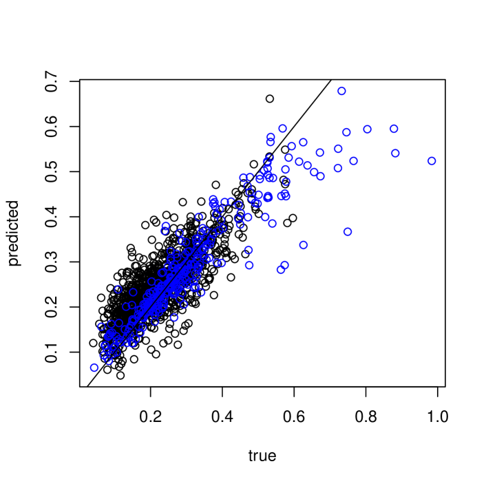
Figure 4: Fit of our model. Black dots are electoral outcomes by local area, while blue dots are exit polling (survey-based) state-level results by age, sex, and education.

We obtained state-level exit polling data obtained from foxnews.com for the following demographics: age, sex, and education. We used these to increase the size and diversity of our sample. In addition to the 979 geographic regions labeled with election outcome data, we used a total of 249 state-level subgroups, e.g. women in Florida, calculating the subgroup feature vectors as described above by restricting to the individual’s in the census matching the demographic reported in the exit poll. As shown in Figure 4 in the Appendix, our model is not overfitting, either to true outcome data (black) or exit poll data (blue). The best $\alpha$ parameter we found was 0.05 (where $0$ is pure ridge regression). The number of parameters in the best model was 415 out of a total of 11,112 features. Using this model, we made predictions for a variety of groups derived from the census, as detailed in the next section.

4 Results: inferring who voted with ecological inference

We start by highlighting the local inferences that our method allows. We inferred the gender gap of support for Trump among men minus support for Trump among women (11 percentage points nationally) for each of 979 geographic regions. As shown in Figure 1 gender gap varies spatially, with some regions showing parity and others exceeding the national average—29 regions had gaps of more than 20 percentage points and 54 regions had negative gender gaps (higher support for Clinton among men than women).

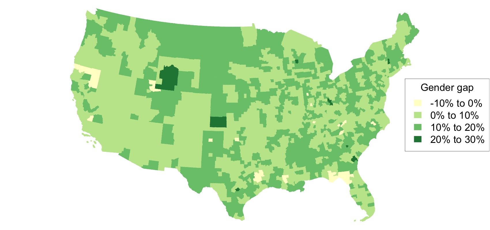
Figure 1: Gender gap in support for Trump represented as percentage point difference between support for Trump among men minus support for Trump among women

In this section we show exit poll-style results which we inferred using the ecological inference methods described above. We could have presented these as contingency tables, but we prefer to mimic the way that exit polls are often presented in the popular press. Here is how to read Table 1, for example. Nationally, among voters who voted for either Trump or Clinton, we estimate that 45% of men voted for Clinton while 55% of men voted for Trump. These two columns will always sum to 1 within a row. The third column says that we estimated that men made up 47% of the electorate, while women made up 53% of the electorate. The column “Participation Rate” gives the percent of voting-age men/women who voted for either Clinton or Trump. The column Other / non-voting is 1-Participation Rate as it gives the percentage of voting-age men/women who voted for a third party or did not vote.

The tables give national results for categories usually reported in exit polls. A variety of other groupings are included in the Appendix in Section B CSV files with all of our estimates are available at the local level on our github repository.

	Clinton	Trump	Fraction of electorate	Participation Rate	Other / Non-voting
Men	0.45	0.55	0.47	0.50	0.50
Women	0.56	0.44	0.53	0.53	0.47
18–29 year olds	0.62	0.38	0.17	0.42	0.58
30–44	0.54	0.46	0.25	0.54	0.46
45–64	0.46	0.54	0.39	0.58	0.42
65 and older	0.45	0.55	0.18	0.47	0.53

Table 1: Estimated demographic trends using our model. Columns show support for Clinton, Trump, fraction of the electorate made up by men (first row) vs women (second row), fraction of voting-age citizens who voted for Clinton or Trump, and fraction of voting-age citizens who voted for a third party or did not vote.

	Clinton	Trump	Fraction of electorate	Participation Rate	Other / Non-voting
Educational attainment
High-school or less	0.47	0.53	0.20	0.25	0.75
Some college	0.46	0.54	0.33	0.49	0.51
Bachelor’s degree	0.51	0.49	0.30	0.84	0.16
Postgraduate education	0.58	0.42	0.17	0.85	0.15
Race/Ethnicity
hispanic	0.68	0.32	0.09	0.43	0.57
white	0.40	0.60	0.72	0.54	0.46
black	0.84	0.16	0.14	0.58	0.42
asian	0.76	0.24	0.03	0.39	0.61
Place of birth
Born in the U.S.	0.42	0.58	0.93	0.62	0.38
U.S. citizen by naturalization	0.74	0.26	0.06	0.42	0.58
Personal income
below $50,000	0.53	0.47	0.64	0.44	0.56
$50,000 to $100,000	0.46	0.54	0.25	0.72	0.28
more than $100,000	0.45	0.55	0.11	0.77	0.23

Table 2: Estimated demographic trends using our model for various census variables. Columns show support for Clinton, Trump, fraction of the electorate made up by men (first row) vs women (second row), fraction of voting-age citizens who voted for Clinton or Trump, and fraction of voting-age citizens who voted for a third party or did not vote.

5 Results: group-based exploratory data analysis

In order to explore which parameters were correlated with the outcome, we used penalized multinomial distribution regression using the same setup as above restricted to subsets of related categorical parameters, e.g. there are 6 different categories for marital status, as shown in Figure 3(b). In each case, we calculated the crossvalidated deviance for the multinomial logistic likelihood, which is a measure of fit allowing different models with different numbers of parameters to be compared. Smaller deviance is better. In Table 3 we show the top 25 performing features.

	feature	deviance	frac.deviance
1	RAC3P - race coding	0.04	0.86
2	ethnicity interacted with has degree	0.04	0.74
3	schooling attainment	0.04	0.72
4	ANC2P - detailed ancestry	0.04	0.83
5	OCCP - occupation	0.04	0.75
6	COW - class of worker	0.04	0.67
7	ANC1P - detailed ancestry	0.05	0.77
8	NAICSP - industry code	0.05	0.71
9	RAC2P - race code	0.05	0.70
10	age interacted with usual hours worked per week (WKHP)	0.05	0.69
11	sex interacted with ethnicity	0.05	0.65
12	MSP - marital status	0.05	0.61
13	FOD1P - field of degree	0.05	0.61
14	ethnicity	0.06	0.57
15	RAC1P - recoded race	0.06	0.54
16	sex interacted with age	0.06	0.57
17	has degree interacted with age	0.06	0.55
18	age interacted with personal income	0.06	0.76
19	sex interacted with hours worked per week	0.06	0.62
20	personal income interacted with hours worked per week	0.06	0.69
21	personal income	0.06	0.59
22	RACSOR - single or multiple race	0.07	0.42
23	has degree interacted with hours worked per week	0.07	0.59
24	hispanic	0.07	0.56
25	sex interacted with personal income	0.07	0.57

Table 3: Lower deviance values indicate a better fit. Larger fraction of deviance explained values are better. Models are fit to the outcome data as described in the text using only the categorical predictors or interactions of categorical predictors listed.

We visualize the marginal effects of the most informative categorical features in Figures 2 and 3, considering not just their predictive ability for Clinton vs. Trump but also their predictive ability in terms of voting for other / not voting, labeling “Participation Rate” to mean the fraction of eligible voters in a category who voted for either Trump or Clinton, thus combining both nonvoters and those who voted for a third-party candidate. In Figure 2, for example, whites with college degrees participated highly and mostly supported Clinton. Whites without college degrees did not participate as highly and mostly supported Trump. Sizes of each buble represent the approximate relative size of each subgroup. For race, occupation, and education level, we show only the most-populous subgroups.

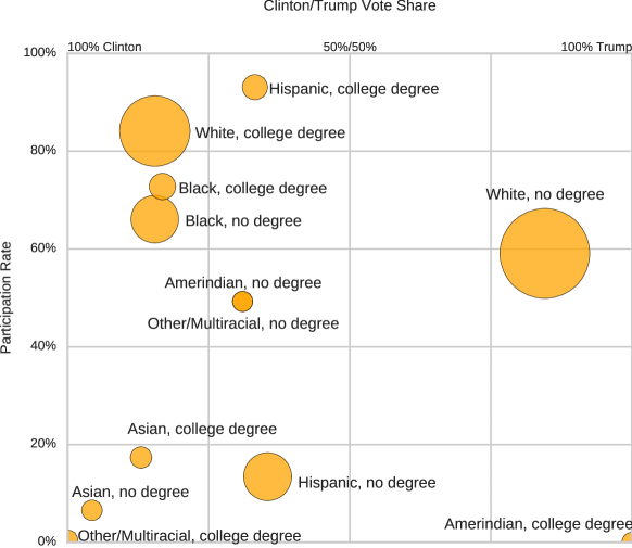
Figure 2: Ethnicity-has degree

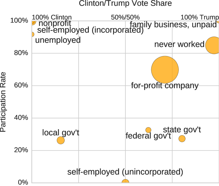
(a) Class of worker COW

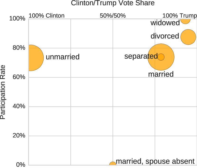
(b) Marital status MSP

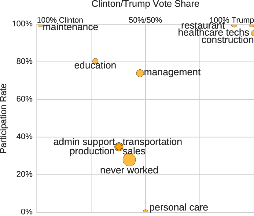
(c) Occupation OCCP

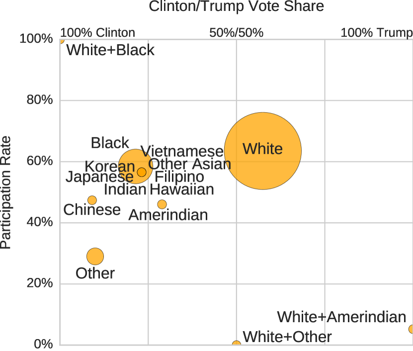
(d) Race RAC3P

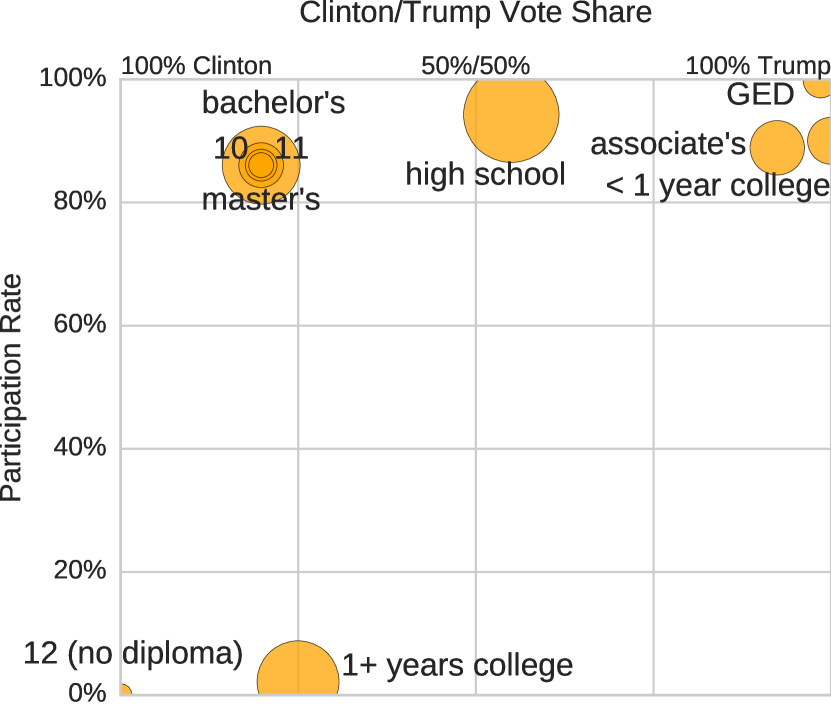
(e) Education level SCHL

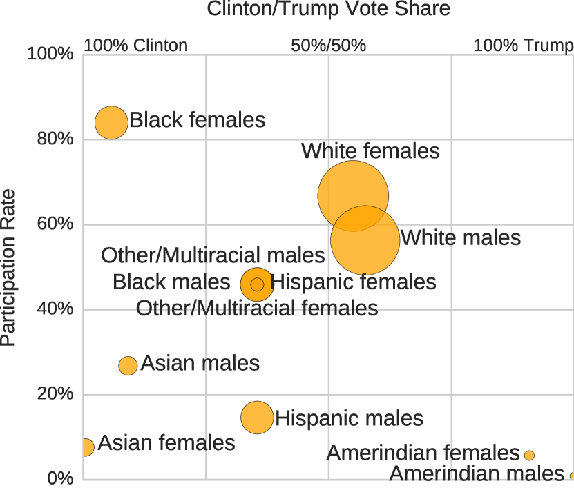
(f) Sex-ethnicity

Figure 3: Several categorical features’ estimated marginal effects on outcomes.

6 Conclusions

This is a work in progress—we are sharing it before the analysis is complete in order to get feedback and in the hopes that it can inform the thinking and analysis of others. In particular, we intend to make comparisons to 2012 data. We will also further explore the wealth of variables in the American Community Survey, add fine-grained spatial maps to complement the demographic modeling in Section 4 and visualize the distributions of real-valued covariates for the most important features discovered in Section 5. Finally, we will consider Bayesian alternatives to the penalized MLE approach in Section 5 so as to, e.g. infer posterior uncertainty regions over the location of our estimates in the square plots.

Appendix A Model fit

Appendix B Supplementary results

	Clinton	Trump	Part.	Other / Non-voting
Hearing difficulty	0.37	0.63	0.47	0.53
Vision difficulty	0.42	0.58	0.46	0.54
Independent living difficulty	0.50	0.50	0.28	0.72
Veteran service connected disability rating (percentage) $\geq$ 10%	0.07	0.93	0.82	0.18
Cognitive difficulty	0.52	0.48	0.23	0.77
Ability to speak English = well	0.73	0.27	0.31	0.69
Ability to speak English = not well or not at all	0.67	0.33	0.21	0.79
Gave birth to a child within the past 12 months	0.51	0.49	0.64	0.36
Grandparents living with grandchildren	0.46	0.54	0.44	0.56
Grandparents responsible for grandchildren	0.42	0.58	0.53	0.47
Insurance purchased directly from an insurance company	0.43	0.57	0.59	0.41
Medicare, for people 65 and older, or people with certain disabilities	0.44	0.56	0.46	0.54
Medicaid or similar	0.56	0.44	0.27	0.73
TRICARE or other military health care	0.26	0.74	0.72	0.28
VA used ever	0.21	0.79	0.70	0.30
Indian Health Service	0.69	0.31	0.22	0.78

	Clinton	Trump	Part	Other / Non-voting
Language other than English spoken at home	0.74	0.26	0.32	0.68
Mobility = lived here one year ago	0.45	0.55	0.55	0.45
Mobility = moved here from outside US and Puerto Rico	0.60	0.40	0.47	0.53
Mobility = moved here from inside US or Puerto Rico	0.56	0.44	0.48	0.52
Active duty military	0.45	0.55	0.56	0.44
Not enrolled in school	0.45	0.55	0.60	0.40
Enrolled in a public school or public college	0.61	0.39	0.39	0.61
Enrolled in private school, private college, or home school	0.66	0.34	0.53	0.47

	Clinton	Trump	Frac	Part	Other / Non-voting
18 $<$= age $<$= 29 & men	0.55	0.45	0.08	0.39	0.61
18 $<$= age $<$= 29 & women	0.71	0.29	0.08	0.37	0.63
30 $<$= age $<$= 44 & men	0.43	0.57	0.13	0.56	0.44
30 $<$= age $<$= 44 & women	0.55	0.45	0.14	0.58	0.42
45 $<$= age $<$= 64 & men	0.48	0.52	0.16	0.49	0.51
45 $<$= age $<$= 64 & women	0.58	0.42	0.21	0.61	0.39
age $>$= 65 & men	0.36	0.64	0.10	0.57	0.43
age $>$= 65 & women	0.49	0.51	0.10	0.48	0.52

	Clinton	Trump	Fraction	Participation	Other
hispanic men	0.66	0.34	0.04	0.39	0.61
white men	0.39	0.61	0.36	0.57	0.43
black men	0.77	0.23	0.05	0.44	0.56
amerindian men	0.50	0.50	0.00	0.28	0.72
asian men	0.74	0.26	0.01	0.37	0.63
hispanic women	0.71	0.29	0.04	0.39	0.61
white women	0.48	0.52	0.38	0.57	0.43
black women	0.87	0.13	0.07	0.61	0.39
amerindian women	0.50	0.50	0.00	0.26	0.74
asian women	0.79	0.21	0.02	0.40	0.60

	Clinton	Trump	Frac	Part	Other / Non-voting
personal income $<$= 50000 & men	0.56	0.44	0.25	0.37	0.63
personal income $<$= 50000 & women	0.63	0.37	0.36	0.40	0.60
50000 $<$ personal income $<$= 100000 & men	0.40	0.60	0.15	0.67	0.33
50000 $<$ personal income $<$= 100000 & women	0.53	0.47	0.13	0.84	0.16
personal income $>$ 100000 & men	0.49	0.51	0.08	0.70	0.30
personal income $>$ 100000 & women	0.62	0.38	0.03	0.80	0.20

References

- Felix et al. (2016) X Yu Felix, Ananda Theertha Suresh, Krzysztof Choromanski, Daniel Holtmann-Rice, and Sanjiv Kumar. Orthogonal random features. 2016.
- Flaxman et al. (2015) Seth Flaxman, Yu-Xiang Wang, and Alexander J Smola. Who Supported Obama in 2012?: Ecological inference through distribution regression. In Proceedings of the 21th ACM SIGKDD International Conference on Knowledge Discovery and Data Mining, pages 289–298. ACM, 2015.
- Gastner et al. (2005) Michael T Gastner, Cosma Rohilla Shalizi, and Mark EJ Newman. Maps and cartograms of the 2004 us presidential election results. Advances in Complex Systems, 8(01):117–123, 2005.
- Gretton et al. (2012) Arthur Gretton, Karsten M Borgwardt, Malte J Rasch, Bernhard Schölkopf, and Alexander Smola. A kernel two-sample test. The Journal of Machine Learning Research, 13:723–773, 2012.
- Lopez-Paz et al. (2015) David Lopez-Paz, Krikamol Muandet, Bernhard Schölkopf, and Ilya Tolstikhin. Towards a learning theory of cause-effect inference. In Proceedings of the 32nd International Conference on Machine Learning, JMLR: W&CP, Lille, France, 2015.
- Smola et al. (2007) Alex Smola, Arthur Gretton, Le Song, and Bernhard Schölkopf. A hilbert space embedding for distributions. In Algorithmic Learning Theory, pages 13–31. Springer, 2007.
- Szabo et al. (2015) Z. Szabo, A. Gretton, B. Poczos, and B. Sriperumbudur. Two-stage Sampled Learning Theory on Distributions. Artificial Intelligence and Statistics (AISTATS), February 2015.