Formation and Fractionation of CO (carbon monoxide) in diffuse clouds observed at optical and radio wavelengths

Abstract

We modelled $\mathrm{{\rm H}_{2}}$ and CO formation incorporating the fractionation and selective photodissociation affecting CO when A_V $\lesssim 2$mag. UV absorption measurements typically have N($\mathrm{{}^{12}CO}$)/N($\mathrm{{}^{13}CO}$) $\approx 65$ that are reproduced with the standard UV radiation and little density dependence at n(H) $\approx 32-1024~{}{\rm cm}^{-3}$: Densities n(H) $\lesssim 256~{}{\rm cm}^{-3}$ avoid overproducing CO. Sightlines observed in mm-wave absorption and a few in UV show enhanced $\mathrm{{}^{13}CO}$ by factors of 2-4 and are explained by higher n(H) $\gtrsim 256~{}{\rm cm}^{-3}$ and/or weaker radiation. The most difficult observations to understand are UV absorptions having N($\mathrm{{}^{12}CO}$)/N($\mathrm{{}^{13}CO}$) $>$100 and N(CO)$\gtrsim 10^{15}~{}{\rm cm}^{-2}$. Plots of ${\rm W}_{\rm CO}$ vs. N(CO) show that ${\rm W}_{\rm CO}$ remains linearly proportional to N(CO) even at high opacity owing to sub-thermal excitation. $\mathrm{{}^{12}CO}$ and $\mathrm{{}^{13}CO}$ have nearly the same curve of growth so their ratios of column density/integrated intensity are comparable even when different from the isotopic abundance ratio. For n(H)$\gtrsim 128~{}{\rm cm}^{-3}$, plots of ${\rm W}_{\rm CO}$ vs N(CH) are insensitive to n(H), and ${\rm W}_{\rm CO}$/N(CO)$\approx 1\mathrm{\,K\,km\,s^{-1}}/(10^{15}~{}{\rm CO}~{}{\rm cm}^{-2})$: This compensates for small CO/$\mathrm{{\rm H}_{2}}$ to make ${\rm W}_{\rm CO}$ more readily detectable. Rapid increases of N(CO) with n(H), N(H) and N($\mathrm{{\rm H}_{2}}$) often render the CO bright, ie a small CO-$\mathrm{{\rm H}_{2}}$ conversion factor. For n(H) $\lesssim 64~{}{\rm cm}^{-3}$ CO enters the regime of truly weak excitation where ${\rm W}_{\rm CO}$$\propto$n(H)N(CO). ${\rm W}_{\rm CO}$ is a strong function of the average $\mathrm{{\rm H}_{2}}$ fraction and models with ${\rm W}_{\rm CO}$=1$\mathrm{\,K\,km\,s^{-1}}$ fall in the narrow range $<{\rm f}_{\mathrm{{\rm H}_{2}}}>$0̄.65-0.8, or $<{\rm f}_{\mathrm{{\rm H}_{2}}}>$0̄.4-0.5 at ${\rm W}_{\rm CO}$0̄.1$\mathrm{\,K\,km\,s^{-1}}$. The insensitivity of easily-detected CO emission to gas with small $<{\rm f}_{\mathrm{{\rm H}_{2}}}>$ implies that even deep CO surveys using broad beams may not discover substantially more emission.

1 Introduction

Carbon monoxide (CO) can form, be shielded and survive in detectable quantities inside even a very modest H I-$\mathrm{{\rm H}_{2}}$ transition in diffuse clouds at A_V $\leq$ 1 mag where C⁺ is the dominant form of gas-phase carbon (Burgh et al., 2010) and as little as a few percent of the total hydrogen column is in the form of $\mathrm{{\rm H}_{2}}$ (Burgh et al., 2007; Sonnentrucker et al., 2007; Sheffer et al., 2008). In UV absorption, CO is detectable when N(CO) $\lesssim 10^{12}~{}{\rm cm}^{-2}$ at N($\mathrm{{\rm H}_{2}}$) $\approx 10^{19}~{}{\rm cm}^{-2}$ and N(H) $\approx$ N(H I) + 2N($\mathrm{{\rm H}_{2}}$) $\approx 2\times 10^{20}~{}{\rm cm}^{-2}$ (Crenny & Federman, 2004). Such small CO column densities are far below those at which mm-wave CO emission becomes detectable at typical sky survey sensitivities${\rm W}_{\rm CO}$ = 1 K-kms (Dame et al., 2001), which is N(CO) $\approx 10^{15}~{}{\rm cm}^{-2}$ (Lucas & Liszt, 1998; Liszt, 2007a).

So it has long been possible to infer that mm-wave CO emission could not trace all of the $\mathrm{{\rm H}_{2}}$-bearing gas in the diffuse molecular interstellar medium (ISM) where cool neutral atomic and molecular hydrogen coexist in appreciable quantities. How much of the diffuse interstellar molecular hydrogen exists in such regions is a question in its own right. It also bears on the question of “dark” gas generally, where the presence of more gas is indicated by gamma-rays or dust emission/extinction than would ordinarily be inferred from 21cm H I and mm-wave CO emission (Grenier et al., 2005; Planck Collaboration et al., 2011, 2015). The gas shortfall has been variously attributed to optically thick H I that is underrepresented in H I emission (Fukui et al., 2015, but see Stanimirović et al. (2014)) or to $\mathrm{{\rm H}_{2}}$ that is missed in CO emission (Wolfire et al., 2010).

Here we discuss the question of just what CO emission traces when the sightline is in the diffuse/translucent domain (roughly, A_V$<$ 2 mag), where C⁺ is the dominant carrier of gas-phase carbon, the gas is somewhat warmer (30 - 80 K) but at typical thermal pressure p/k $\gtrsim 2-3\times 10^{3}~{}{\rm cm}^{-3}$ K (Jenkins & Tripp, 2011) so that CO is weakly excited by ambient $\mathrm{{\rm H}_{2}}$ (Liszt, 2007a) and, in some cases, heavily fractionated (Liszt & Lucas, 1998) owing to chemical isotope exchange (Watson et al., 1976; Smith & Adams, 1980) and selective photodissociation (Bally & Langer, 1982; Van Dishoeck & Black, 1988; Warin et al., 1996; Visser et al., 2009). These effects act simultaneously to produce isotoplogic abundance ratios that sometimes show the dominance of one or the other mechanism but may also result in normal-seeming abundance ratios that conceal the complex nature of the underlying physical processes.

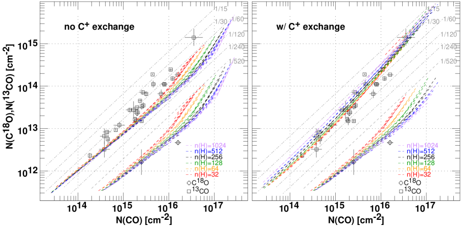
Figure 1: Carbon monoxide column densities modelled with (right) and without C⁺ exchange. In both panels N($\mathrm{{}^{13}CO}$) and N($\mathrm{C^{18}O}$) are plotted against N(CO) with UV-absorption observations shown as hollow rectangles and diamonds, respectively. In each panel model results are shown for densities n(H) = 32 .. 1024$~{}{\rm cm}^{-3}$ varying in steps of two. The calculations were taken from spherical clump models in which the central column density N(H) was varied in steps of $2^{1/4}$ and for each model two values, corresponding to sightlines at the center and the geometric mean impact parameter, are connected by a dashed line . In each panel, ratios with respect to the main isotope are shown as shaded dashed lines.

Interpretation of CO emission is quite particular in the diffuse/translucent regime because the isotopologues can not be presumed to be present in the same proportions as the inherent atomic isotope ratios, so the line brightnesses of the isotopologues cannot be compared with the inherent elemental abundance ratios to directly derive the line optical depths and column densities. Even so, the CO column densities would be of little use in inferring N($\mathrm{{\rm H}_{2}}$) when most of the carbon is in the form of neutral atomic carbon or C⁺, and the CO abundance relative to $\mathrm{{\rm H}_{2}}$ is small (ie $<<10^{-4}$) and highly variable with respect to small changes in the ambient conditions (Szucs et al., 2016). At the same time, as we discuss below, sub-thermal excitation puts the J=1-0 rotational line in a radiative transfer regime where the isotopologic line brightnesses are proportional to their respective column densities even for very optically thick lines (Goldreich & Kwan, 1974), so the ratios of brightnesses reflect the ratio of abundance even when the observed values (say 15:1 for $\mathrm{{}^{12}CO}$/$\mathrm{{}^{13}CO}$) would under other circumstances just be taken as evidence for heavily saturated $\mathrm{{}^{12}CO}$ emission.

The plan of this work is as follows. In Section 2 we describe the computational devices used to calculate $\mathrm{{\rm H}_{2}}$ and CO abundances and CO line brightnesses. In Section 3 we compare models of the CO formation, excitation and fractionation with UV- and radio absorption line measurements where the most complete knowledge of $\mathrm{{\rm H}_{2}}$ and CO column densities is available. In large part this is done in order to understand what is implied by the differences in fractionation that apparently occur between sightlines toward bright early-type stars used in UV-absorption and those used in the mm-wave regime toward distant blazars. But it also serves the necessary purpose of benchmarking the models against the lines of sight where the most complete information on CO and $\mathrm{{\rm H}_{2}}$ is available, which seems necessary before discussing In Section 4 we discuss CO emission more generally, to correspond to the more usual case that only CO emission is observed in one or more isotopologues. Section 5 is a summary and overview.

2 Model calculations

Discussion of CO formation and fractionation in diffuse $\mathrm{{\rm H}_{2}}$-bearing gas proceeds in several steps: i) description of the underlying physical properties of the host gas; ii) the $\mathrm{{\rm H}_{2}}$-formation and $\mathrm{{\rm H}_{2}}$ self-shielding mechanism in the otherwise-atomic medium; iii) the formation chemistry of the carbon monoxide isotopologues and their photodissociation, self- and mutual shielding and chemical carbon isotope exchange (Warin et al., 1996; Visser et al., 2009); iv) calculation of the brightness of the CO lines and the effect of CO radiation on the overall energy balance and temperature distribution: This is generally negligible here.

2.1 Heating, cooling and geometry

As in our previous work, we adopt the heating-cooling model of Wolfire et al. (2003) at the Solar circle, as incorporated into a spherical cloud with uniform density. The cloud is embedded in the ambient, isotropic, galactic radiation field of photons and cosmic-rays, with the default rate of the latter taken as $\mbox{$\zeta_{H}$}=2\times 10^{-16}\mbox{~{}s${}^{-1}$}$ per H-nucleus as seems appropriate for the diffuse molecular ISM (McCall et al., 2002; Liszt, 2003; Hollenbach et al., 2012; Indriolo et al., 2012, 2015). Most of the heating is from the photoelectron effect on small grains and the cooling is through excitation of the fine structure lines of C⁺ and O I. Rev2: The optical/UV radiation field is that of Draine (1978), scaled overall by a factor G₀ whose default value is unity. The equations of chemical and thermal balance are solved iteratively over a computational model with 128 or more equi-spaced radial shells, computing the radiation field in each shell averaged over the surrounding 4$\pi$ solid angle. This formulation was recently used to study the formation and self-shielding of HD and $\mathrm{{\rm H}_{2}}$ under conditions of varying metallicity (Liszt, 2015).

2.2 $\mathrm{{\rm H}_{2}}$ formation and self-shielding

Following the prescription of (Spitzer, 1978, see also Sternberg et al. (2014)) the rate constant for $\mathrm{{\rm H}_{2}}$-formation on grain surfaces is taken as R_G $=3\times 10^{-18}~{}{\rm cm}^{3}\mbox{~{}s${}^{-1}$}\sqrt{\mbox{$T_{K}$}}$ where $T_{K}$ is the locally-computed kinetic temperature. However, the thermal balance and temperature-dependent rate constant are not of crucial importance to the $\mathrm{{\rm H}_{2}}$-fraction. Very nearly the same results are obtained using a fixed rate constant R_G $=3.9\times 10^{-17}~{}{\rm cm}^{3}\mbox{~{}s${}^{-1}$}$ that is the average of the values obtained toward three stars by Gry et al. (2002) and is often cited in other work, see Liszt (2015). The most important point overall is to reproduce the observed mean $\mathrm{{\rm H}_{2}}$-derived kinetic temperature $\approx$ 80 K (Savage et al., 1977; Rachford et al., 2002) at the typical thermal pressures p/k $\approx 3000~{}{\rm cm}^{-3}$ K (Jenkins & Tripp, 2011) that are appropriate for the $\mathrm{{\rm H}_{2}}$-bearing regions.

The models employ the $\mathrm{{\rm H}_{2}}$ photodissociation and self-shielding scheme of Draine & Bertoldi (1996) which explicitly treats dust attenuation of the radiation field at the wavelengths of the Lyman and Werner bands of $\mathrm{{\rm H}_{2}}$ (90 - 110 nm). The optical depth for dust absorption is $\tau_{d}$ = $1.9\times 10^{-21}$N(H) (Draine, 2003) as in Sternberg et al. (2014). The free-space photodissocation rate of $\mathrm{{\rm H}_{2}}$ is $4.25\times 10^{-11}\mbox{G${}_{0}$}\mbox{~{}s${}^{-1}$}$, also as in Sternberg et al. (2014). The accuracy of the Draine & Bertoldi (1996) formulation was recently verified in great detail by Sternberg et al. (2014) using an exact calculation in the context of the Meudon PDR code. Continuous absorption by dust is especially important at densities n(H) $\lesssim 32~{}{\rm cm}^{-3}$ when large hydrogen columns are required before much $\mathrm{{\rm H}_{2}}$ accumulates (Liszt, 2015).

2.3 CO formation

The CO formation chemistry adopted here is extremely simple and direct: CO forms from the thermal recombination of a fixed quantity of $\mathrm{HCO^{+}}$ at the locally-calculated kinetic temperature; more explicitly, there is a constant assumed relative abundance X($\mathrm{HCO^{+}}$) = n($\mathrm{HCO^{+}}$)/n($\mathrm{{\rm H}_{2}}$) = $3\times 10^{-9}$ as inferred from observation (Liszt et al., 2010). The CO isotopologues are assumed to form in proportion to their inherent elemental abundance, which we take as $\mathrm{{}^{12}CO}$:$\mathrm{{}^{13}CO}$:$\mathrm{C^{18}O}$ = 1:1/60:1/520 (Lucas & Liszt, 1998). This reflects the fact that the isotopologues of $\mathrm{HCO^{+}}$ should be present in proportion to the inherent elemental isotopic abundance ratios, given the difficulty of fractionating $\mathrm{HCO^{+}}$ in diffuse gas. $\mathrm{HCO^{+}}$ recombines with an electron many thousands of times faster than it reacts with an ambient $\mathrm{{}^{13}CO}$ molecule, which is the pathway that enhances H¹³CO⁺ in dense, fully-molecular clouds (Roueff et al., 2015).

It is generally agreed that $\mathrm{HCO^{+}}$ recombines to form the CO that is observed in diffuse gas (Visser et al., 2009) but the origin of the $\mathrm{HCO^{+}}$ requires a mechanism that proceeds much faster than the rate of ion-molecule reactions in the gas that is modelled here. As noted below it is one of the insights of this work that the bulk of the UV absorption line data and all of the observations of CO absorption at mm-wavelengths are explained when the formation of CO from $\mathrm{HCO^{+}}$ recombination and the in-situ fractionation and carbon isotope exchange of CO procede at thermal rates.

2.4 CO photodissociation

The CO photodissociation scheme adopted here is that of Visser et al. (2009), numerically based on tables of shielding factors obtained from the website referenced there. The free-space photodissocation rates of the CO isotopologues are $2.6\times 10^{-10}\mbox{G${}_{0}$}\mbox{~{}s${}^{-1}$}$ for $\mathrm{{}^{12}CO}$ and $\mathrm{{}^{13}CO}$, and $2.4\times 10^{-10}\mbox{G${}_{0}$}\mbox{~{}s${}^{-1}$}$ for $\mathrm{C^{18}O}$. The online tables have a much finer granularity (0.2 dex) than those published in the manuscript itself (1 dex). In this scheme both dust and $\mathrm{{\rm H}_{2}}$ shield the isotopologues but CO provides vastly more shielding for the rarer isotopologues than the rarer isotopologues provide for themselves. Therefore the tables use N(CO) as the independent variable for the shielding of all isotopologues. The secondary effect of self-shielding of the rarer ¹³C-bearing isotopologues by themselves is accomodated by a 2nd table dimension that is the relative abundance of the rarer isotopologue, with the value 1:1/35 or 1:1/65; for the ¹⁸O-bearing isotopologues there is only one possibility, 1:1/560. As discussed in Appendix A the shielding factors of Visser et al. (2009) are not always interpreted in this way.

Because the calculations are not performed with the actual local relative isotopologic abundances, we experimented by repeating the same calculations with tables corresponding to the two carbon isotopologic abundance ratios. In the unphysical case that C⁺ isotope exchange is neglected, the shielding table with $\mathrm{{}^{12}CO}$/$\mathrm{{}^{13}CO}$ = 65 is clearly preferable on physical grounds (see Figure 1) but there were only very slight differences of a few percent using the table with the higher $\mathrm{{}^{13}CO}$ abundance. When carbon isotope exchange is included (as it should be), use of both tables gives even much more similar results owing to the strong inter-species coupling. In any case the small differences between the isotopologic ratios in the tables and the in-situ formation rate ratios in our work is of little consequence to the results that are presented.

2.5 Carbon isotope exchange and other chemistry

The process of exothermic (34.8 K) carbon isotope exchange in reactions of ¹³C⁺with CO was introduced by Watson et al. (1976). We adopt the more recent measured, temperature-dependent rate constants of Smith & Adams (1980) as parametrized by Liszt (2007a), see also Roueff et al. (2015). Use of the carbon exchange reaction in various implementations is discussed in Appendix A.

The formation/fractionation chemistry employed here was discussed in an approximate way in Liszt (2007a). The important effects are CO formation, photodissociation, and destruction by He⁺, along with the carbon isotope exchange. We solved a limited chemical network consisting of these effects coupled with the underlying calculation of ionization equilbrium and charge balance of all species that is inherent in the basic heating-cooling calculation. In this way the equilibrium between carbon atoms, ions and CO is explicitly maintained for all the isotopes and isotopologues.

The model sphere calculation is performed radially in 128 equi-spaced shells using a relaxation mechanism that repeatedly recourses inward from the edge to the center until the abundances have converged in each shell and are self- and mutually consistent. The calculation is required to converge in the number densities of $\mathrm{{\rm H}_{2}}$, HD and the CO isotopologues, as well as the kinetic temperature and ionization equilibrium, etc, in each shell. Once the internal radial variation of all quantities is known, the observable column densities and CO line brightnesses can be calculated for any impact parameter about the central sightline. In the figures, we have typically calculated series of models at fixed number density n(H) while varying the front-back total central column density N(H) in steps of $2^{1/4}$, displaying the results for each model as a line segment connecting the results for 0 impact parameter and an impact parameter equal to 2/3 of the radius, which is the geometric mean over the face of the model. As noted in the Introduction the model values for n(H) and N(H) include H-nuclei in all forms, including protons, $\mathrm{{\rm H}_{2}}$⁺, etc. but the fractional abundances of species other than atomic and molecular hydrogen are very small so that N(H) $\approx$ N(H I) + 2 N($\mathrm{{\rm H}_{2}}$).

2.6 The CO J=1-0 emission line brightness and CO cooling

As in Liszt (2007a) the carbon monoxide J=1-0 emission line brightnesses are calculated from a microturbulent approximation with complete redistribution (Leung & Liszt, 1976) and CO cooling is also included in the model although it is negliglible in the presence of so much C⁺. The rotational excitation of CO is implemented as described in Liszt (2007a) including excitation by atomic helium and hydrogen, ortho and para-$\mathrm{{\rm H}_{2}}$, although excitation by atomic hydrogen is actually negligible given the small rate constants (Shepler et al., 2007; Walker et al., 2015) and the absence of CO except when the molecular hydrogen fraction is large. The J=0 and 1 levels of $\mathrm{{\rm H}_{2}}$ are taken to be in thermal equilbrium at the local kinetic temperature (Savage et al., 1977; Rachford et al., 2002). The CO and $\mathrm{{}^{13}CO}$ integrated line profile brightnesses in units of K km s^-1 are written as ${\rm W}_{\rm CO}$ and ${\rm W}_{\rm 13}$ respectively.

2.7 Specific observational results discussed here

Like Visser et al. (2009) we discuss the CO and $\mathrm{{}^{13}CO}$ column densities determined in UV absorption toward bright stars by Sheffer et al. (2007) and Sonnentrucker et al. (2007) and the $\mathrm{C^{18}O}$ column densities of Lambert et al. (1994) and Sheffer et al. (2002). We discuss the CO and $\mathrm{{}^{13}CO}$ column densities determined in mm-wave absorption by Liszt & Lucas (1998) and the emission brightnesses presented there and by Liszt (1997) toward $\zeta$ Oph. We also discuss the CO emission observed toward common UV absorption targets (Liszt, 2008) and the “Mask 1” subset of CO emission brightnesses in Taurus observed by Goldsmith et al. (2008).

2.8 Comparison of approaches to shielding and isotope exchange with other work

Similarities and differences in the self-shielding and carbon isotope exchange schemes used here and other work (Sheffer et al., 2007; Röllig & Ossenkopf, 2013; Szucs et al., 2014; Roueff et al., 2015; Szucs et al., 2016) are discussed in Appendix A.

2.9 A reference value for the CO-H₂ conversion factor

Throughout this work we refer to the CO-$\mathrm{{\rm H}_{2}}$ conversion factor as ${\rm X}_{\rm CO}$ = N($\mathrm{{\rm H}_{2}}$)/${\rm W}_{\rm CO}$ and take as a standard or reference the value ${\rm X}_{\rm CO}^{0}$ $=2\times 10^{20}~{}\mathrm{{\rm H}_{2}}~{}{\rm cm}^{-2}$/(K-km s^-1).

3 Comparison of absorption line observations with models

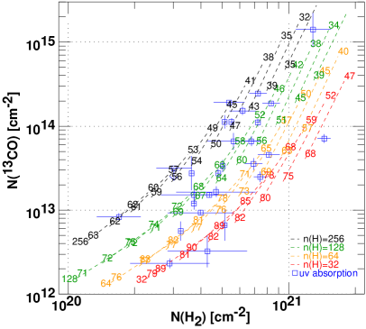
Figure 2: N($\mathrm{{}^{13}CO}$) vs N($\mathrm{{\rm H}_{2}}$) for models shown in Figure 1 with the uv absorption line data superposed as hollow blue rectangles. As in Figure 1 each model is represented by a dashed line segment connecting the values at the center and geometric median impact parameter, but in this figure the N($\mathrm{{}^{12}CO}$)/N($\mathrm{{}^{13}CO}$) ratios are shown at the endpoints of each line segment. The number density n(H) is indicated at the lefthand side of each series of models.

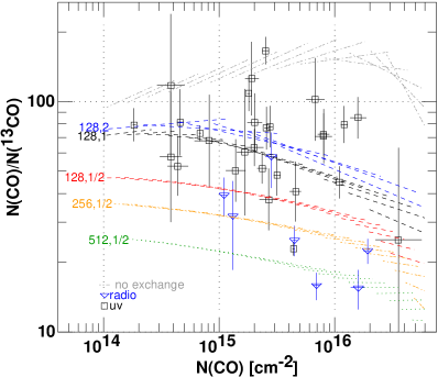
Figure 3: The N($\mathrm{{}^{12}CO}$)/N($\mathrm{{}^{13}CO}$) ratio for optical (hollow black rectangles) and radio (blue downward triangles) absorption line observations, and models with varying number density and scaled radiation field. Each model calculation is labeled with its (n(H),G0) values. The dash-dot loci at the highest N($\mathrm{{}^{12}CO}$)/N($\mathrm{{}^{13}CO}$) ratios correspond to calculations ignoring carbon isotope exchange.

Figure 4: Emission profile integrals for $\mathrm{{}^{12}CO}$ and $\mathrm{{}^{13}CO}$ and model results for n(H)$=128~{}{\rm cm}^{-3},256~{}{\rm cm}^{-3}$ and $512~{}{\rm cm}^{-3}$. The datapoints include sightlines toward early-type stars (Liszt, 2008) (“Survey2008”), pointings within 20^′of $\zeta$ Oph (Liszt, 1997), PdBI sightlines toward compact extragalactic continuum sources (Liszt & Lucas, 1998; Liszt et al., 2010) used for absorption line studies at the Plateau de Bure Interferometer (“PdBI sightlines”) and the “Mask 1” pixels in the Taurus region discussed by Goldsmith et al. (2008). Denoting G0 as usual as the ratio of the optical/UV radiation field to its standard value, models for G0=1,1/2 and 1/3 are shown in each panel as blue, orange and red lines, respectively, and the green dash-dot curve that is lowest in each panel shows model results neglecting isotope exchange. Gray dashed lines show fiducial values 2.5, 5, 10 … 120 of the ${\rm W}_{\rm CO}$/${\rm W}_{\rm 13}$ intensity ratio and numbers along each curve show the actual column density ratio N($\mathrm{{}^{12}CO}$)/N($\mathrm{{}^{13}CO}$). In the middle panel each model is shown as a dotted curve with FWHM linewidth dV = 0.9 km s^-1, dV = 1.3 km s^-1 otherwise.

Figure 1 shows the carbon monoxide column densities derived in UV absorption along with models with and without C⁺ exchange, at right and left, respectively. Note that all of the sightlines have N(CO) $>10^{14.1}~{}{\rm cm}^{-2}$ and so reside in the same regime of CO formation photochemistry initiated by processes involving C⁺ and OH, according to Sheffer et al. (2008). The $\mathrm{{}^{12}CO}$/$\mathrm{{}^{13}CO}$ ratios are for the most part surprisingly well fit by the isotopologic abundance ratio N($\mathrm{{}^{12}CO}$)/N($\mathrm{{}^{13}CO}$) = C/¹³C = 60 that is inherent in the model, while the observed N(CO)/N($\mathrm{C^{18}O}$) ratios are three-five times higher than the intrinsic isotope ¹³C/¹⁸O ratio 520 used in the model.

The observed high N(CO)/N($\mathrm{C^{18}O}$) ratios are fit equally well with or without carbon isotope exchange because $\mathrm{C^{18}O}$ is shielded mainly by $\mathrm{{}^{12}CO}$ whose abundance is little changed. The observed ratios N($\mathrm{{}^{12}CO}$)/N($\mathrm{{}^{13}CO}$) $\approx$ 60 seem to ignore the expected complications of selective photodissociation, carbon isotope exchange and the like. However, this is in no way an indication that carbon isotope exchange and selective photodissociation are not occuring. The models shown at left ignoring carbon isotope exchange generally trace only the very lower envelope of the $\mathrm{{}^{13}CO}$ data, especially at the lower densities, with $\mathrm{{}^{13}CO}$ column densities two-three times lower than observed. The models without isotope exchange at left in Figure 1 produce results very similar to those of the suprathermal chemistry employed by Visser et al. (2009), as discussed in Section 3.1.

Introducing carbon isotope exchange at right in Figure 1 brings the model results into general agreement with the CO and $\mathrm{{}^{13}CO}$ data, with little obvious dependence on the density, because the horizontal axis is N(CO) rather than, say, N($\mathrm{{\rm H}_{2}}$) (see Section 3.1 and Figure 2). The upward curvature in the models is not apparent in the data unless the highest datapoint is considered. The improved fit at higher density for the $\mathrm{{}^{12}CO}$/$\mathrm{C^{18}O}$ ratio toward the star at higher column density occurs because N(H) and N($\mathrm{{\rm H}_{2}}$) are both smaller at higher density for a given N(CO): the $\mathrm{C^{18}O}$ is then less well shielded $\mathrm{{\rm H}_{2}}$ and dust.

The diffuse $\mathrm{{\rm H}_{2}}$-bearing gas seen in UV absorption can be unambiguously distinguished by its high inherent N(CO)/N($\mathrm{C^{18}O}$) ratios that are three-five times larger than the inherent isotope ratio but distinguishing diffuse gas by comparing CO and $\mathrm{{}^{13}CO}$  is far more problematical. Deviations from the inherent isotopic abundance ratio are a clear sign of diffuse/translucent gas whether high or low but only a small proportion of the $\mathrm{{}^{13}CO}$ datapoints are strongly deviant.

3.1 N($\mathrm{{}^{13}CO}$)

The CO formation rate is one of several factors competing to determine the $\mathrm{{}^{12}CO}$/$\mathrm{{}^{13}CO}$ ratio shown in Figure 1, so it is also important to reproduce the isotoplogic ratios at CO/$\mathrm{{\rm H}_{2}}$ abundances that are also like those that are actually observed. If the CO abundance is not reproduced, conclusions regarding the fractionation can be misleading. Figure 2 shows N($\mathrm{{}^{13}CO}$) plotted against N($\mathrm{{\rm H}_{2}}$) with the isotopologic abundance ratio shown at both endpoints of each model’s line segment (connecting the column densities calculated toward the model’s center and geometric-mean impact parameter).

The N($\mathrm{{}^{13}CO}$) and N($\mathrm{{\rm H}_{2}}$) observed in UV absorption line data are reproduced at relatively modest densities $32~{}{\rm cm}^{-3}\lesssim$ n(H) $\lesssim 256~{}{\rm cm}^{-3}$ as with the models in Figure 1. The vertical scatter is much larger in Figure 2: a factor 15-30 at given N($\mathrm{{\rm H}_{2}}$) and with variation of N($\mathrm{{}^{13}CO}$) by a factor exceeding 100 for $3\times 10^{20}~{}{\rm cm}^{-2}\lesssim$ N($\mathrm{{}^{13}CO}$) $\lesssim 7\times 10^{20}~{}{\rm cm}^{-2}$. It can be explained by variations in density and impact parameter as in Figure 2, but variations in the local UV illumination also must contribute.

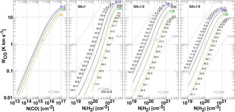
Figure 5: $\mathrm{{}^{12}CO}$ emission profile integrals ${\rm W}_{\rm CO}$ plotted against $\mathrm{{}^{12}CO}$ and $\mathrm{{\rm H}_{2}}$ column densities. Numerical values along curves indicate the ${\rm W}_{\rm CO}$/W₁₃ emission profile brightness ratio. The calculations used a FWHM linewidth dV = 1.3 km s^-1; calculations with dV = 0.9 km s^-1 are shown as dotted lines for two densities in the panel for G0 = 1.

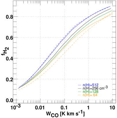
Figure 6: $\mathrm{{\rm H}_{2}}$-fraction plotted as a function of the CO profile integral toward the center of models at four densities n(H) = 64 .. 512 $~{}{\rm cm}^{-3}$. Results are plotted as solid lines for all densities at G0 = 1 and as dashed lines for G0 = 1/2 at the highest and lowest densities. The color scheme is the same as in Figure 1.

3.2 Strongly deviant UV data and the radio-UV comparison

In Figure 1 at right, there are three statistically significant datapoints with N($\mathrm{{}^{12}CO}$)/N($\mathrm{{}^{13}CO}$) ratios well below the inherent carbon isotope ratio and five-six where N($\mathrm{{}^{12}CO}$)/N($\mathrm{{}^{13}CO}$) is substantially larger. Deviations also exist for the mm-wave data (Liszt & Lucas, 1998) but only in one sense and generally opposite to the UV data, with small N($\mathrm{{}^{12}CO}$)/N($\mathrm{{}^{13}CO}$) and favoring chemical fractionation over selective photodissociation. This is shown in Figure 3 where the radio and UV data are compared: Other versions of this figure exist in Liszt (2007a), Sheffer et al. (2007), Visser et al. (2009), and Szucs et al. (2014), also using the results of Liszt & Lucas (1998). With some overlap, the N($\mathrm{{}^{12}CO}$)/N($\mathrm{{}^{13}CO}$) ratio is systematically smaller on sightlines observed at mm-wavelengths that do not specifically target early-type stars and, albeit with a smaller sample, none of the radio datapoints show N($\mathrm{{}^{12}CO}$)/N($\mathrm{{}^{13}CO}$) exceeding the inherent elemental isotopic abundance ratio of 60.

The radio or UV data with N($\mathrm{{}^{12}CO}$)/N($\mathrm{{}^{13}CO}$) $<60$ are easily accomodated with modest (factor two) increases in density and/or smaller radiation fields. However, increasing the radiation field or decreasing the density causes rather small changes in the N(CO)-N($\mathrm{{}^{13}CO}$) curves and the most problematic data are those observed in the UV for which N($\mathrm{{}^{12}CO}$)/N($\mathrm{{}^{13}CO}$) $>80$. Shown in Figure 3 as an upper envelope is the model result for n(H) $=128~{}{\rm cm}^{-3}$ neglecting carbon isotope exchange that is also shown at left in Figure 1. The largest N($\mathrm{{}^{12}CO}$)/N($\mathrm{{}^{13}CO}$) ratio, toward the archetypal line of sight to $\zeta$ Oph, is at the very margin of the values calculated ignoring carbon isotope exchange.

Figures 1-3 allow a direct comparison with the chemical calculations of Visser et al. (2009) from which our shielding factors were drawn. Because Visser et al. (2009) drove the isotope exchange reaction at suprathermal rates, with an effective temperature 4000 K, the 35 K zero-point energy difference between CO and $\mathrm{{}^{13}CO}$ was ineffective, and their results generally resemble those shown at left in Figure 1 here. For instance, the earlier chemistry gave N($\mathrm{{}^{12}CO}$)/N($\mathrm{{}^{13}CO}$) $\approx 140$ at N($\mathrm{{\rm H}_{2}}$) $\approx 4-5\times 10^{20}~{}{\rm cm}^{-2}$ while the curves shown in our Figure 2 have N($\mathrm{{}^{12}CO}$)/N($\mathrm{{}^{13}CO}$) $\approx 50-85$ over that same range. The N($\mathrm{{}^{13}CO}$)/N($\mathrm{{\rm H}_{2}}$) ratios in the earlier work are smaller than those shown in our Figure 2.

3.3 Summing up; thermal and suprathermal chemistry

Although our models including carbon isotope exchange cannot account for the handful of sightlines observed in UV absorption and having N($\mathrm{{}^{12}CO}$)/N($\mathrm{{}^{13}CO}$) $\gtrsim 80$ at N(CO) $>10^{15}~{}{\rm cm}^{-2}$ (see Figure 3), effective carbon isotope exchange at thermal rates is needed to explain the bulk of the UV observations and all of the data at mm-wavelengths. The recombination of $\mathrm{HCO^{+}}$ to form CO and the carbon isotope exchange affecting the N($\mathrm{{}^{12}CO}$)/N($\mathrm{{}^{13}CO}$) ratio can be understood as occurring at thermal rates after the formation of $\mathrm{HCO^{+}}$, however that occurs. As noted in Section 3 in reference to Figure 1, all of the sightlines considered here in UV absorption have N(CO) $>10^{14.1}~{}{\rm cm}^{-2}$ and should be subject to the same formation photochemistry according to the discussion of Sheffer et al. (2008).

As they discussed, high ratios N($\mathrm{{}^{12}CO}$)/N($\mathrm{{}^{13}CO}$) occur as a matter of course in the suprathermal chemistry of Visser et al. (2009). If the N($\mathrm{{}^{12}CO}$)/N($\mathrm{{}^{13}CO}$) ratio is high because the carbon isotope exchange reaction were ad hoc being driven at suprathermal rates with high effective temperatures 4000 K along some lines of sight, the recombination of $\mathrm{HCO^{+}}$ to form CO would also presumably occur more slowly owing to the inverse temperature dependence of recombination rates generally. For a given N(CO) this would in turn imply that X($\mathrm{HCO^{+}}$) is higher in about the same proportion that its recombination rate to form CO is diminished.

The $\mathrm{HCO^{+}}$ column density cannot be measured directly along the sightlines studied in UV absorption, but the combination of higher N($\mathrm{HCO^{+}}$) and somewhat stronger $\mathrm{HCO^{+}}$-electron excitation at higher temperature would presumably produce brighter $\mathrm{HCO^{+}}$ rotational emission where the N($\mathrm{{}^{12}CO}$)/N($\mathrm{{}^{13}CO}$) ratio was exceptionally large. CO, $\mathrm{{}^{13}CO}$ and $\mathrm{HCO^{+}}$ emission have all been observed toward and around $\zeta$ Oph where the N($\mathrm{{}^{12}CO}$)/N($\mathrm{{}^{13}CO}$) ratio is highest in UV absorption and the gas seen in emission is in the foreground of the star (Wilson et al., 1992; Kopp et al., 1996; Liszt, 1997). Toward the star, ${\rm W}_{\rm CO}$ $\approx 1.5$ K-km s^-1 and $\mathrm{{}^{13}CO}$ emission is at best marginally detectable with ${\rm W}_{\rm CO}$/${\rm W}_{\rm 13}$ $\gtrsim 60$ (Wilson et al., 1992). $\mathrm{HCO^{+}}$ emission is present at a level 2.2% that of ${\rm W}_{\rm CO}$, typical of sightlines observed in $\mathrm{HCO^{+}}$ absorption and emission in diffuse molecular gas at mm-wavelengths (Lucas & Liszt, 1996): It is not exceptionally strong.

CO, $\mathrm{{}^{13}CO}$ and $\mathrm{HCO^{+}}$ all brighten considerably within 10^′-30^′ to the north and south of $\zeta$ Oph with the CO/$\mathrm{HCO^{+}}$ brightness ratio staying about constant at 50-100 while ${\rm W}_{\rm CO}$/${\rm W}_{\rm 13}$ decreases to 20-30. $\mathrm{HCO^{+}}$ emission tracks ${\rm W}_{\rm CO}$ fairly closely and varies with ${\rm W}_{\rm CO}$ in the same sense as ${\rm W}_{\rm 13}$. This seems opposite to expectations if the suprathermal chemistry causes high effective kinetic termperatures in interactions of $\mathrm{HCO^{+}}$ with electrons while retarding the carbon exchange reaction of C⁺ with CO.

4 CO emission in the face of fractionation

In the vast majority of cases, observations of carbon monoxide are those made in mm-wave emission without recourse to either absorption spectra or independent knowledge of N($\mathrm{{\rm H}_{2}}$), etc: The integrated brightness of CO is often the independent variable or a constituent of it (eg when N(H) is approximated as N(H) = N(H I)+ 2 ${\rm X}_{\rm CO}$${\rm W}_{\rm CO}$). Measurements of $\mathrm{{}^{13}CO}$ emission in identifiably-diffuse gas are scarce but, in an attempt to show the equivalent of Figure 1 in emission, Figure 4 shows measurements of CO and $\mathrm{{}^{13}CO}$ emission from our work at the Plateau de Bure (Liszt & Lucas, 1998), from a survey of carbon monoxide emission toward commonly-used UV absorption background targets (Liszt, 2008), from data within 20^′ of $\zeta$ Oph (Liszt, 1997) and from the lowest-A_V “Mask 1” pixels of Goldsmith et al. (2008) in Taurus.

The panels show results toward the centers of models at n(H) = 128, 256 and 512 $~{}{\rm cm}^{-3}$ with the radiation field at full strength and diluted by factors of 2 and 3. Each model curve is shown solid with FWHM = dV = 1.3 km s^-1 and dotted in the middle panel with dV = 0.9 km s^-1. Fiducial values 2.5, 5, 10, 20 … of the ${\rm W}_{\rm CO}$/${\rm W}_{\rm 13}$ integrated intensity ratio are plotted as dashed gray lines, and dash-dotted in green we show the calculated emission when carbon isotope exchange is ignored for G0 = 1. Numerical values of the column density ratio N($\mathrm{{}^{12}CO}$)/N($\mathrm{{}^{13}CO}$) are shown along each model curve: These can be compared with the fiducial lines to gauge the extent to which the intensity and column density ratios differ owing to radiative transfer effects. Varying the density has relatively little effect on the model brightnesses in Figure 4 when the radiation field is at full strength, consistent with the lack of density sensitivity shown in Figure 1 at right. For weaker illumination ${\rm W}_{\rm CO}$/${\rm W}_{\rm 13}$ decreases with n(H), and moreso as the illumination diminishes.

The emission observations accompanying the PdBI absorption data are explained by some combination of higher density and dimmer radiation, as in Figure 3 where the UV and mm-wave absorption line data were compared. The Taurus data “Mask 1” pixels of Goldsmith et al. (2008) are consistent with the other datasets, with $1/15\leq\mbox{${\rm W}_{\rm 13}$}/\mbox{${\rm W}_{\rm CO}$}\leq 1/30$. It is interesting that the Taurus observations, which isolate diffuse sightlines within a dark cloud complex, are consistent with observations along sightlines observed at high latitudes at the PdBI that are supposedly remote from dense or dark gas. $\mathrm{{}^{13}CO}$ emission is often quite bright toward the early-type stars even though the UV absorption line data generally show smaller N($\mathrm{{}^{13}CO}$)/N(CO) ratios than in the radio domain (ie Figure 3). Strong carbon monoxide emission toward early-type stars almost certainly arises from dense material with high A_V situated behind the star. Had the stars in question been located behind such material they would have too heavily extincted to be suitable absorption line targets.

${\rm W}_{\rm CO}$/${\rm W}_{\rm 13}$ intensity ratios are (perhaps) surprisingly close to the column density ratios N($\mathrm{{}^{12}CO}$)/N($\mathrm{{}^{13}CO}$) even when both are small compared to the intrinsic carbon isotope ratio 60: For ${\rm W}_{\rm CO}$ $\lesssim$ 4 K, the differences between the column density and brightness ratios are 25% or less. Differences are larger for brighter lines and for lower density, but small intensity ratios reflect comparably small column density ratios, even when ${\rm W}_{\rm CO}$/${\rm W}_{\rm 13}$ $\approx 10-20$. For instance the Taurus results with ${\rm W}_{\rm CO}$/${\rm W}_{\rm 13}$ in the range 13 - 22 are reproduced in the right-most panel by the models with n(H) $=512~{}{\rm cm}^{-3}$, G0 = 1/2 and column density ratios N($\mathrm{{}^{12}CO}$)/N($\mathrm{{}^{13}CO}$) in the range 19 - 26, or in the center panel at n(H)$=256~{}{\rm cm}^{-3}$ with G0 $\gtrsim$ 1/3 and N($\mathrm{{}^{12}CO}$)/N($\mathrm{{}^{13}CO}$) in the range 16 - 22. Close tracking of the intensity and column density ratios requires that the J=1-0 brightness maintains a proportionality to the column density well beyond the point at which the optical depth exceeds unity, as we now discuss.

4.1 ${\rm W}_{\rm CO}$ vs. ${\rm N}_{\rm CO}$: The curve of growth

Figure 5 shows the CO brightness plotted against N(CO) at left for G0 = 1 and n(H) = 64, 128, 256 and 512 $~{}{\rm cm}^{-3}$, and against N($\mathrm{{\rm H}_{2}}$) at the same n(H) for G0 = 1, 1/2, and 1/3 in the three rightmost panels. The variation of ${\rm W}_{\rm CO}$ with N(CO) haa little sensitivity to the radiation field. Values of ${\rm W}_{\rm CO}$/${\rm W}_{\rm 13}$ are superposed numerically on the model curves in the rightmost panels where fiducial values of the CO-$\mathrm{{\rm H}_{2}}$ conversion factor N($\mathrm{{\rm H}_{2}}$)/${\rm W}_{\rm CO}$ in units of $\mathrm{{\rm H}_{2}}\ ~{}{\rm cm}^{-2}$/(K-km s^-1) are indicated as gray, dashed lines.

In the left-hand panel of Figure 5 the plots of ${\rm W}_{\rm CO}$ vs N(CO) show that ${\rm W}_{\rm CO}$ (K-km s^-1) $\approx$ N(CO)/$10^{15}~{}{\rm cm}^{-2}$ around ${\rm W}_{\rm CO}$ = 1 K-km s^-1 for n(H) $\gtrsim 128~{}{\rm cm}^{-3}$ and ${\rm W}_{\rm CO}$ $\approx$ N(CO)/$2\times 10^{15}~{}{\rm cm}^{-3}$ for n(H) $=64~{}{\rm cm}^{-3}$. These are comparatively low densities to be discussing, even in the context of CO emission at the sensitivity limit of typical survey observations. For n(H) $\lesssim 64~{}{\rm cm}^{-3}$, CO is increasingly in the true limit of weak collisional excitation where n($\mathrm{{\rm H}_{2}}$)N(CO) is constant (Liszt & Pety, 2016).

When the excitation is weak and the rotational energy ladder is well below the level of thermalization, the J=1-0 brightness remains proportional to the CO column density long after the J=1-0 line becomes optically thick at with $\tau\gtrsim 1$ at N(CO) $\gtrsim 10^{15}~{}{\rm cm}^{-2}$: This is because the radiative transfer is dominated by scattering. Moreover, the ratio ${\rm W}_{\rm CO}$/N(CO) is comparatively large in diffuse gas (Liszt, 2007a; Liszt et al., 2010), some 30- 50 times higher than in cold dark clouds or when the rotational ladder is thermalized, because so much of the energy in the rotation ladder emerges in the 1-0 lowest transition. This behaviour was predicted by Goldreich & Kwan (1974) long before it was inferred from observation by direct comparison of ${\rm W}_{\rm CO}$ and N(CO). As discused in Section 5 a higher ${\rm W}_{\rm CO}$/N(CO) ratio compensates for smaller CO/$\mathrm{{\rm H}_{2}}$ ratios in diffuse gas, such that ${\rm W}_{\rm CO}$/N($\mathrm{{\rm H}_{2}}$) tends to remain constant between regions of high and low X(CO). The ${\rm W}_{\rm CO}$/N($\mathrm{{\rm H}_{2}}$) ratio in diffuse gas differs much less than the ${\rm W}_{\rm CO}$/N(CO) ratio because the fractional abundance of CO is so small.

4.2 N($\mathrm{{\rm H}_{2}}$)/${\rm W}_{\rm CO}$: the CO-H₂ conversion factor

The right-hand three panels of Figure 5 show ${\rm W}_{\rm CO}$ vs N($\mathrm{{\rm H}_{2}}$) for G0 = 1, 1/2 and 1/3 with model results for n(H) = 64 .. 512 $~{}{\rm cm}^{-3}$. Casting the discussion in terms of ${\rm W}_{\rm CO}$ and N($\mathrm{{\rm H}_{2}}$) lends itself to discussion of the ${\rm W}_{\rm CO}$-N($\mathrm{{\rm H}_{2}}$) conversion factor which is schematically illustrated in the figure by the gray dashed fiducial lines.

The models in Figure 5 have an approximately quadratic dependence ${\rm W}_{\rm CO}$ $\propto$ N($\mathrm{{\rm H}_{2}}$)^1.5-2 and N($\mathrm{{\rm H}_{2}}$) $=2.1\times 10^{20}~{}{\rm cm}^{-2}$ around ${\rm W}_{\rm CO}$ = 1 K-km s^-1 for G0=1 and n(H) = 256 $~{}{\rm cm}^{-3}$. ${\rm W}_{\rm CO}$ varies more rapidly than linearly with N($\mathrm{{\rm H}_{2}}$) at fixed number density owing to the fast increase of N(CO) with N($\mathrm{{\rm H}_{2}}$) and this rapid increase of ${\rm W}_{\rm CO}$ with N($\mathrm{{\rm H}_{2}}$) means that CO-$\mathrm{{\rm H}_{2}}$ conversion factors ${\rm X}_{\rm CO}$ $<$ ${\rm X}_{\rm CO}^{0}$ often apply when ${\rm W}_{\rm CO}$ $\gtrsim 1$ K km s^-1. This is “bright’ CO Liszt & Pety (2012), and CO is increasingly bright in this sense at higher density and for smaller G0.

The CO-$\mathrm{{\rm H}_{2}}$ conversion factor ${\rm X}_{\rm CO}$ = N($\mathrm{{\rm H}_{2}}$)/${\rm W}_{\rm CO}$scales directly with G0 (${\rm X}_{\rm CO}$/G0 $\approx$ constant), and inversely with density (${\rm X}_{\rm CO}$ $\propto$ n(H)^-0.75) and with ${\rm W}_{\rm CO}$ itself, ${\rm X}_{\rm CO}$$\propto 1/\mbox{${\rm W}_{\rm CO}$}^{0.3-0.5}$ with a slightly stronger dependence on ${\rm W}_{\rm CO}$ at higher G0. The variation of ${\rm W}_{\rm CO}$ with N($\mathrm{{\rm H}_{2}}$) shown in Figure 5 can be approximated around ${\rm W}_{\rm CO}$ = 1 K-km s^-1 and inverted to give

$$N(\mathrm{{\rm H}_{2}})=Ay^{b}\times\mbox{${\rm W}_{\rm CO}$}^{1/{(c+d{\rm ln}(y))}}$$

where y = n(H)$/256~{}{\rm cm}^{-3}$, ${\rm W}_{\rm CO}$ is measured in K-km s^-1 and constants for the evaluation of Equation 1 are given in Table 1. The functional dependence is very nearly as G0/n(H) that is the fundamental scaling parameter for PDR in general.

Table 1: Constants for the evaluation of Equation 1

G0	A	b	c	d
1	2.24 $\times 10^{20}$ $\mathrm{{\rm H}_{2}}$ (K-km s-1)-1	-0.74	1.92	-0.35
1/2	1.0 $\times 10^{20}$ $\mathrm{{\rm H}_{2}}$ (K-km s-1)-1	-0.79	1.66	-0.12
1/3	0.69 $\times 10^{20}$ $\mathrm{{\rm H}_{2}}$ (K-km s-1)-1	-0.76	1.51	-0.08

In discussing Figure 4 we noted that our models with G0 = 1/2-1/3 and n(H) = 256 $~{}{\rm cm}^{-3}$ or G0 $\approx$ 1/2 and n(H) = 512 $~{}{\rm cm}^{-3}$ reproduce the ${\rm W}_{\rm CO}$ and ${\rm W}_{\rm 13}$ measurements from which N(CO) and N($\mathrm{{\rm H}_{2}}$) were derived for the Mask 1 pixels in Taurus of Goldsmith et al. (2008). Our model with G0 = 0.5 and n(H) = 512 $~{}{\rm cm}^{-3}$ in Figure 5 has the same CO-$\mathrm{{\rm H}_{2}}$ conversion factor but five times smaller N(CO) and N($\mathrm{{\rm H}_{2}}$) than were derived by Goldsmith et al. (2008). This occurs because the gas in our models is substantially warmer and the excitation more strongly sub-thermal than was assumed by Goldsmith et al. (2008), which brightens the CO emission on a per-molecule basis while reproducing the observed ${\rm W}_{\rm CO}$ with a smaller CO column density, as discussed by Liszt et al. (2010).

4.3 Practical limitations on the utility of CO emission as an $\mathrm{{\rm H}_{2}}$ tracer

Figure 6 gathers results for models of varying density and G0 and plots the line of sight averaged molecular hydrogen fraction $<{\rm f}_{\mathrm{{\rm H}_{2}}}>$ against ${\rm W}_{\rm CO}$. At the typical survey limit ${\rm W}_{\rm CO}$ = 1 K-km s^-1, the models cluster in the narrow range $<{\rm f}_{\mathrm{{\rm H}_{2}}}>$ = 0.65 - 0.8, large but still with a significant component of atomic hydrogen, falling only to $<{\rm f}_{\mathrm{{\rm H}_{2}}}>$ = 0.45 - 0.6 at ${\rm W}_{\rm CO}$ = 0.1 K-km s^-1. This suggests that the known CO emission arises in material where the hydrogen has mostly been converted to molecular form and that even much deeper CO searches will not reveal much more emission except perhaps at higher spatial resolution.

This is not to say how much $\mathrm{{\rm H}_{2}}$ is missed by CO surveys at the current $\approx$ 1 k-km s^-1 sensitivity limit, because that depends on the distribution of cloud properties . Most of the $\mathrm{{\rm H}_{2}}$ could reside in regions with a high enough molecular fraction that CO is detectable, though we noted earlier that there could be a substantial population of H I clouds with high column density and low number density and molecular fraction (Liszt, 2007b). Global estimates of $<{\rm f}_{\mathrm{{\rm H}_{2}}}>$ in the diffuse ISM based on absorption line observations range from $\gtrsim 22$% measured in $\mathrm{{\rm H}_{2}}$ and corrected for sampling bias (Savage et al., 1977; Bohlin et al., 1978), to 35-40% assuming constancy of the observed mean chemical abundances X($\mathrm{HCO^{+}}$) $=3\times 10^{-9}$ (Liszt et al., 2010) and X(CH) $=3.5\times 10^{-8}$ (Liszt & Lucas, 2002). In any case, the associated CO is not inferred to be abnormally dim Liszt et al. (2010).

5 Summary and discussion

We began by describing in Section 2 a physical scheme for numerical calculation of the abundances of the carbon monoxide isotopolgues $\mathrm{{}^{12}CO}$, $\mathrm{{}^{13}CO}$ and $\mathrm{C^{18}O}$ in uniform density gas spheres of modest total extinction and densities n(H) = 32 - 1024 $~{}{\rm cm}^{-3}$. The models self-consistently compute the equilibrium state considering heating and cooling of the host gas along with the $\mathrm{{\rm H}_{2}}$ formation, self- and dust shielding in the otherwise-atomic medium; CO formation via the thermal recombination of a fixed relative abundance X($\mathrm{HCO^{+}}$) = n($\mathrm{HCO^{+}}$)/n($\mathrm{{\rm H}_{2}}$) $=3\times 10^{-9}$; and CO photodissociation, self- and mutual shielding and carbon isotope exchange. The emergent line intensities of the CO J=1-0 transition are calculated in the microturbulent approximation.

In Section 3, as a benchmark, we compared the model calculations with UV observations of CO in absorption. Figure 1, displaying results for models with and without carbon isotope exchange, shows that the observed isotopologic ratios N($\mathrm{{}^{12}CO}$)/N($\mathrm{{}^{13}CO}$) are generally well-reproduced over the full range N($\mathrm{{}^{12}CO}$) $=2\times 10^{14}-4\times 10^{16}~{}{\rm cm}^{-2}$ and that the near-constancy of N($\mathrm{{}^{12}CO}$)/N($\mathrm{{}^{13}CO}$) $\approx$ 65 at N($\mathrm{{}^{12}CO}$) $\lesssim 2\times 10^{16}~{}{\rm cm}^{-2}$, near the intrinsic ¹²C/¹³C ratio, in fact results from a complex interaction of shielding, selective photodissociation and carbon isotope exchange processes. When carbon isotope exchange is considered, the model results inter-comparing the various CO isotopologues have little dependence on number density although with some preference for the highest density to explain one of only two datapoints for the rarer isotopologue $\mathrm{C^{18}O}$.

Because the isotopologic abundance ratios depend on the proper balance between formation, destruction and exchange processes we took care to verify that the CO isotopologic abundance ratios were reproduced at the observed column densities (Section 3.1 and Figure 2). The number density should be moderate, n(H) $\lesssim 256~{}{\rm cm}^{-2}$, to avoid over-producing CO along sightlines observed in UV absorption and to maintain consistency with the rotational excitation temperatures that are an indirect by-product of measurements of CO absorption in the UV (Smith et al., 1978; Crutcher & Watson, 1981; Wannier et al., 1982; Crenny & Federman, 2004; Liszt, 2007a; Goldsmith, 2013). At such densities CO acounts for 5 - 20% of the gas-phase carbon in the center of models with N(H) = $1-2\times 10^{21}~{}{\rm cm}^{-2}$ (A_V $\approx$ 1/2 - 1 mag) as discussed in Appendix B and illustrated in Figure B1.

Some deviant datapoints were discussed in Section 3.2. Smaller N($\mathrm{{}^{12}CO}$)/N($\mathrm{{}^{13}CO}$) ratios can be explained by weakening the UV-illumination by factors of 2-3 and by increasing the density, but the converse is not true: High ratios N($\mathrm{{}^{12}CO}$)/N($\mathrm{{}^{13}CO}$) $>80$ are not reproduced by increasing the strength of the illumination. In Figure 3 we compared the results for CO absorption observed at optical and radio wavelengths, noting that the radio data have systematically smaller N($\mathrm{{}^{12}CO}$)/N($\mathrm{{}^{13}CO}$) ratios. This indicates that that they arise in conditions involving some combination of higher density and weaker UV illumination than is characteristic of the foreground material observed toward early-type stars.

High N($\mathrm{{}^{12}CO}$)/N($\mathrm{{}^{13}CO}$) ratios, in the range 100 - 160, are seen only along sightlines used to study UV absorption. As shown in Figure 3, the largest N($\mathrm{{}^{12}CO}$)/N($\mathrm{{}^{13}CO}$) ratios can be reproduced by suppressing the carbon isotope exchange, as occurs in suprathermal chemistries like that of Visser et al. (2009). In Section 3.3 we argued that suppressing carbon isotope exchange via a suprathermal chemistry would imply slower $\mathrm{HCO^{+}}$ recombination to CO, requiring a larger N($\mathrm{HCO^{+}}$)/N(CO) ratio and brighter $\mathrm{HCO^{+}}$ mm-wave emission relative to that of CO. However, observations of CO, $\mathrm{{}^{13}CO}$, and $\mathrm{HCO^{+}}$ emission toward and around $\zeta$ Oph, where the N($\mathrm{{}^{12}CO}$)/N($\mathrm{{}^{13}CO}$) is highest in the UV, show a more or less constant $\mathrm{HCO^{+}}$/CO brightess ratio around the star, even as ${\rm W}_{\rm CO}$/${\rm W}_{\rm 13}$ falls to 20-30.

In Section 4 we turned attention to CO emission on its own terms, to discuss the most common case where only emission from one of more isotopologues is available and independent information on, for instance, N($\mathrm{{\rm H}_{2}}$) is not available. In Figure 4 we showed observations of $\mathrm{{}^{12}CO}$ and $\mathrm{{}^{13}CO}$ emission in identifiably-diffuse directions and compared them with models at n(H) $=128-512~{}{\rm cm}^{-3}$ and G0 = 1/3 - 1. The CO emission data toward the same stars used for UV absorption are often dominated by background gas having relatively strong $\mathrm{{}^{13}CO}$ emission, because of selection biases against high foreground extinction. Observations toward outlying portions of the Taurus cloud are consistent with the other datasets (an important point given the supposed absence of high-A_V material in the vicinity of the sighlines studied in mm-wave absorption) and are well-explained with n(H) $=512~{}{\rm cm}^{-3}$ and twice weaker UV illumination or n(H) $=256~{}{\rm cm}^{-3}$ and three times weaker UV illumination. The CO brightness and column density ratios are comparable even when they are much different from the inherent atomic isotope ratio: Small ${\rm W}_{\rm CO}$/${\rm W}_{\rm 13}$ ratios imply small N($\mathrm{{}^{12}CO}$)/N($\mathrm{{}^{13}CO}$) ratios and small CO/$\mathrm{{\rm H}_{2}}$ abundance ratios rather than a saturation of the emission from the more abundant isotopologue.

In Section 4.1 we considered the CO curve of growth for CO emission, the variation of ${\rm W}_{\rm CO}$ witn N(CO) noting that the emission brightness per CO molecule around ${\rm W}_{\rm CO}$ = 1 K-km s^-1 is ${\rm W}_{\rm CO}$/N(CO) $\approx$ 1 K-km s^-1$/10^{15}~{}{\rm cm}^{-2}$ for n(H) $\geq 128~{}{\rm cm}^{-3}$ or ${\rm W}_{\rm CO}$/N(CO) $\approx$ 0.5 K-km s^-1$/10^{15}$(n(H)/64$~{}{\rm cm}^{-3}$)$~{}{\rm cm}^{-2}$ for n(H) $\leq 64~{}{\rm cm}^{-3}$. The ${\rm W}_{\rm CO}$/N(CO) ratio is relatively high in diffuse gas because nearly all the energy put into the CO rotation ladder by collisions emerges in the J=1-0 transition. Moreover, ${\rm W}_{\rm CO}$ $\propto$ N(CO) even at N(CO) $>10^{15}~{}{\rm cm}^{-2}$ where the J=1-0 line has $\tau\approx 1$, because the CO gas is effectively a pure scattering environment. The density dependence in the ${\rm W}_{\rm CO}$/N(CO) ratio at n(H) $\lesssim 64~{}{\rm cm}^{-2}$ is a sign that CO is entering the limit of truly weak collisional excitation formulated by Linke et al. (1977) and Liszt & Pety (2016).

In Figure 5 at right we showed calculated results for ${\rm W}_{\rm CO}$ vs. N($\mathrm{{\rm H}_{2}}$), which allowed a discussion of the CO-$\mathrm{{\rm H}_{2}}$ conversion factor N($\mathrm{{\rm H}_{2}}$)/${\rm W}_{\rm CO}$ in Section 4.2 where we parametrized the dependence of N($\mathrm{{\rm H}_{2}}$) on ${\rm W}_{\rm CO}$ in equation 1 and Table 1. The rapid increase of N(CO) with density and N($\mathrm{{\rm H}_{2}}$), combined with the proportionality between N(CO) and ${\rm W}_{\rm CO}$, causes much of the CO emission at levels ${\rm W}_{\rm CO}$ $\gtrsim$ 1 K-km s^-1 to be ’bright’ in the sense of having a CO-$\mathrm{{\rm H}_{2}}$ conversion factor N($\mathrm{{\rm H}_{2}}$)/${\rm W}_{\rm CO}$ smaller than the ’standard’ value ${\rm X}_{\rm CO}^{0}$ $=2\times 10^{20}~{}\mathrm{{\rm H}_{2}}~{}{\rm cm}^{-2}$/(K-km s^-1).

In Section 4.3 (see Figure 6) we discussed how molecular emission at the level ${\rm W}_{\rm CO}$ = 1 K-km s^-1 arises from gas in a narrow range of line-of-sight averaged $\mathrm{{\rm H}_{2}}$-fraction $<{\rm f}_{\mathrm{{\rm H}_{2}}}>$ = 0.65 - 0.8, only falling to $<{\rm f}_{\mathrm{{\rm H}_{2}}}>$ = 0.45 - 0.6 at 0.1 K-km s^-1. Easily detectable CO emission does not occur in gas except where $\mathrm{{\rm H}_{2}}$ is the dominant form of hydrogen. This probably implies that CO searches at levels well below ${\rm W}_{\rm CO}$ = 1 K-km s^-1 with broad beams will not detect much more CO emission. However, CO emission is heavily clumped on arcminute and smaller scales and quite bright patches may well exist within broad beams lacking detectable emission at levels 1 K-km s^-1 (Heithausen, 2006; Liszt & Pety, 2012).

How much diffuse molecular gas has been missed by the existing CO surveys is a separate question but the fact that the average CO-$\mathrm{{\rm H}_{2}}$ conversion factor in diffuse molecular gas is near-standard (Liszt et al., 2010) indicates that most of the $\mathrm{{\rm H}_{2}}$ in the diffuse ISM exists in regions with sufficiently large local f${}_{\mathrm{{\rm H}_{2}}}$ that CO emission should be detectable. In any case it appears that detection of $\mathrm{{\rm H}_{2}}$ in regions with very small $<{\rm f}_{\mathrm{{\rm H}_{2}}}>$ $<<$ 0.5 is best left to absorption line measurements of species like OH⁺ which actually prefer such conditions and perhaps to observation of species like CH, OH and $\mathrm{HCO^{+}}$, whose abundances with respect to $\mathrm{{\rm H}_{2}}$ are not as sensitive to ambient conditions as that of CO (Gerin et al., 2016).

5.1 Discussion

We discussed the optical/UV/radio absorption line data in order to establish the suitability of the underlying models before extrapolating to cases where CO emission alone will be used to infer N($\mathrm{{\rm H}_{2}}$) and few if any constraints are available. To this end we note especially that the bulk of that data is understandable in terms of a chemistry that occurs at thermal rates, after $\mathrm{HCO^{+}}$ forms: specifically, this work invoked the thermal recombination of the observed amount of $\mathrm{HCO^{+}}$ with electrons to form the observed amounts of carbon monoxide, and the carbon isotope exchange that is required to explain $\mathrm{{}^{12}CO}$/$\mathrm{{}^{13}CO}$ ratios that are below or only modestly above the inherent isotopic abundance ratio. Some UV sightlines do not entirely conform to this picture because their CO column densities are reproduced, at least approximately, even while N($\mathrm{{}^{12}CO}$)/N($\mathrm{{}^{13}CO}$) has high values that only seem attainable if carbon isotope exchange is suppressed. Overall, however, and toward all the sightlines observed in absorption at mm-wavelengths, far from early-type stars and presumably more typical, carbon isotope exchange fractionation dominates over selective photodissociation. The great majority of the $\mathrm{{}^{13}CO}$ observed in diffuse molecular gas arises through the deposition of ¹³C into CO, rather than the direct formation of $\mathrm{{}^{13}CO}$ via the recombination of H¹³CO⁺. This situation is directly comparable to that of the HD in the diffuse ISM, which results from the deposition of deuterons into existing $\mathrm{{\rm H}_{2}}$ rather than the formation of HD on grains directly.

As shown in Figure 5 at left, the quantity that is most directly and reliably inferred from observations of CO emission in diffuse molecular gas is N(CO) because the emission brightness per CO molecule around ${\rm W}_{\rm CO}$ = 1 K-km s^-1, ${\rm W}_{\rm CO}$/N(CO) $\approx$ 1 K-km s^-1$/10^{15}~{}{\rm cm}^{-2}$, is insensitive to the illumination of the gas, and insensitive to the number density when n(H) $\gtrsim 128~{}{\rm cm}^{-3}$, or ${\rm W}_{\rm CO}$/N(CO) $\approx$ 0.5 K-km s^-1$/10^{15}~{}{\rm cm}^{-2}$ (n(H)/64$~{}{\rm cm}^{-3}$) for n(H) $\lesssim 64~{}{\rm cm}^{-3}$.

In this regime N($\mathrm{{}^{12}CO}$)/N($\mathrm{{}^{13}CO}$) $\approx$ ${\rm W}_{\rm CO}$/${\rm W}_{\rm 13}$ even when small values of ${\rm W}_{\rm CO}$/${\rm W}_{\rm 13}$ might seem to imply substantial saturation of the CO emission with unfractionated column density ratios.

Failure to recognize that N($\mathrm{{}^{12}CO}$)/N($\mathrm{{}^{13}CO}$) $\approx$ ${\rm W}_{\rm CO}$/${\rm W}_{\rm 13}$, and that this implies that CO carries a small fraction of the gas-phase carbon, can lead to serious errors when deriving molecular gas properties. Just this point has recently been addressed by Szucs et al. (2016) who concluded that the least reliable way to infer N($\mathrm{{\rm H}_{2}}$) is to calculate N($\mathrm{{}^{13}CO}$) and thereafter to compute N(CO) and N($\mathrm{{\rm H}_{2}}$) without knowing the isotopologue ratio N($\mathrm{{}^{12}CO}$)/N($\mathrm{{}^{13}CO}$) and CO abundance. They conclude that use of a standard CO-$\mathrm{{\rm H}_{2}}$ conversion factor applied to ${\rm W}_{\rm CO}$ is more reliable. In fact something very like this point was made long ago at a time when the CO-$\mathrm{{\rm H}_{2}}$ conversion factor had not yet entered the mainstream and N($\mathrm{{\rm H}_{2}}$) was determined by calculating N($\mathrm{{}^{13}CO}$) in LTE at a temperature inferred from CO, and multiplying N($\mathrm{{}^{13}CO}$) by the ratio appropriate for fully-molecular gas, N($\mathrm{{\rm H}_{2}}$)/N($\mathrm{{}^{13}CO}$) $\approx 5\times 10^{5}$ (Dickman, 1978). As noted then, it is possible to arrive at a value for N($\mathrm{{\rm H}_{2}}$) with much less effort and no more uncertainty simply as N($\mathrm{{\rm H}_{2}}$) = ${\rm X}_{\rm CO}$ ${\rm W}_{\rm CO}$ using a standard value for ${\rm X}_{\rm CO}$ (Liszt, 1984).

Appendix A Comparison of approaches to CO shielding and C⁺ exchange

Recent work incorporates carbon monoxide photodissociation and/or fractionation in chemical studies that cover rather different physical regimes from that considered here, although with some consideration of results for CO column densities measured in UV absorption as shown here in Figure 1. Röllig & Ossenkopf (2013) discuss carbon fractionation chemistry in PDR with n(H) = $10^{3}-10^{7}~{}{\rm cm}^{-3}$ while Szucs et al. (2014) discuss carbon monoxide chemistry in turbulent clouds of typical mass 10⁴ M_Sun and mean density n(H) = 300 $~{}{\rm cm}^{-3}$, equivalent in some rough sense to a uniform sphere of radius R=7 pc and central column density 2n(H)R $=1.27\times 10^{22}~{}{\rm cm}^{-2}$ or A_V = 7 mag, well beyond the range of column density considered here.

Unlike the current work, Röllig & Ossenkopf (2013) and Szucs et al. (2014) find noticeable and very similar enhancement of ¹³CO at all values of N(CO) below the point where all carbon is in CO, for instance with $15\lesssim$ N($\mathrm{{}^{12}CO}$)/N($\mathrm{{}^{13}CO}$) $\lesssim 40$ for $10^{13}~{}{\rm cm}^{-2}\lesssim$ N(CO) $\lesssim 10^{17}~{}{\rm cm}^{-2}$. As noted by Szucs et al. (2014) in regard to their Figure 14, equivalent to our Figure 3, their results are much better suited to comparison with our mm-wave absorption results (Liszt & Lucas, 1998) and the UV absorption results must reflect different conditions than those that were considered. In the present work the difference is attributed to higher density and weaker UV illumination along sightlines removed from early-type stars.

In fact these differences arise from differing treatment of carbon monoxide self-shielding and fractionation, as we now discuss.

A.1 Self and mutual shielding

Röllig & Ossenkopf (2013) used the shielding factors tabulated by Van Dishoeck & Black (1988) that were calculated and tabulated in a form similar to those of Visser et al. (2009) so their results would be most nearly comparable to those presented here. However, Röllig & Ossenkopf (2013) reinterpreted the basic spectroscopic scheme behind the shielding calculations that have been performed by van Dishoeck and her collaborators, in which the shielding of all the isotopologues ${}^{x}C^{y}O$ is expressed as functions of N($\mathrm{{\rm H}_{2}}$) and N($\mathrm{{}^{12}CO}$), not of N($\mathrm{{\rm H}_{2}}$) and N(${}^{x}C^{y}O$), etc. The ratios N(${}^{x}C^{y}O$)/N($\mathrm{{}^{12}CO}$) are secondary parameters of limited significance in the formulation of Visser et al. (2009). Thus footnote 11 of Röllig & Ossenkopf (2013) states that “$\mathrm{{}^{12}CO}$ could also shield its less abundant relatives, if their absorption lines are sufficiently close together. However, only very few of the efficiently dissociating lines overlap, too few for mutual shielding to be important (Warin et al., 1996).” However, the footnote to Table 5 of self-shieldings in Visser et al. (2009) makes explicit that “Self-shielding is mostly negligible for the heavier isotopologues, so all shielding functions are expressed as a function of the $\mathrm{{}^{12}CO}$ column density.” This reflects a fundamental disagreement between the microphysics of line overlap between Warin et al. (1996) and Van Dishoeck & Black (1988) or Visser et al. (2009).

The first preprint version of Szucs et al. (2014) that we downloaded when initially drafting this manuscript adopted the same self-shielding formulation of Lee et al. (1996) that we used in our own earlier work when only $\mathrm{{}^{12}CO}$ was discussed, and they modelled the shielding of $\mathrm{{}^{13}CO}$ by substituting N($\mathrm{{}^{13}CO}$) for N($\mathrm{{}^{12}CO}$): That is, both isotopologues use the same shielding factors, but the column density employed to calculate the shielding of ^xC^yO was N(^xC^yO) as in the scheme of Röllig & Ossenkopf (2013). The final published version uses the shielding factors of Visser et al. (2009) but presumably with the same scheme of self-shielding of the heavier isotopologues, rather than by $\mathrm{{}^{12}CO}$. This presumably also is true of the successor work by Szucs et al. (2016).

A.2 The carbon-exchange reaction rate

Yet another difference with the present work is that Szucs et al. (2014) (and, presumably Szucs et al. (2016)) used a single value for the forward rate constant (ie that for the exothermic replacement of C by ¹³C in CO), as measured at 300 K by Watson et al. (1976). In doing so they followed a remark by Sheffer et al. (2007) to the effect that the older result provided a better fit to the UV absorption line observations, a few of which have high N($\mathrm{{}^{12}CO}$)/N($\mathrm{{}^{13}CO}$) ratios. We, along with Röllig & Ossenkopf (2013) (also see Roueff et al. (2015)) approximated the temperature-dependent rate coefficients for C⁺ exchange measured by Smith & Adams (1980). These are higher than the value $k_{f}=2\times 10^{-10}{\rm cm}^{3}$ s^-1 of Watson et al. (1976) by factors of 2, 3 and 4 at at kinetic temperatures 160 K, 80 K, and 30 K, respectively.

Appendix B Internal structure

Figure B1 shows the internal structure of our cloud models with N(H) = $1\times 10^{21}~{}{\rm cm}^{-2}$ and $2\times 10^{21}~{}{\rm cm}^{-2}$ at top and bottom, respectively. The CO column densities toward the centers of these models vary from $8.1\times 10^{13}~{}{\rm cm}^{-2}$ to $1.3\times 10^{16}~{}{\rm cm}^{-2}$ at top (a factor 160 vs. 8 in density) and from $8.8\times 10^{14}~{}{\rm cm}^{-2}$ to $8.3\times 10^{16}~{}{\rm cm}^{-2}$ at bottom. For comparison with Figures 1 and 3, the central CO column densities at n(H) $=128~{}{\rm cm}^{-3}$ are $1.1\times 10^{15}~{}{\rm cm}^{-2}$ at top and $1.1\times 10^{16}~{}{\rm cm}^{-2}$ at bottom.

The temperature distribution is nearly uniform because the models are relatively transparent (A_V = 0.25 and 0.5 at the center) and the CO fraction – the CO abundance relative to the free gas-phase carbon abundance – is generally small. The temperature at the center of the densest model at bottom increases toward the center as C⁺ becomes a minority constituent and CO cooling does not make up the difference. The outer temperature varies from 55 K to 100 K as the density decreases from $512~{}{\rm cm}^{-2}$ to $32~{}{\rm cm}^{-2}$. The thermal pressure p/k $\approx 3\times 10^{3}~{}{\rm cm}^{-3}$K at n(H) $=32~{}{\rm cm}^{-3}$ was a basic constraint on the underlying heating-cooling calculation. The thermal pressure of the highest density models is 4 times higher than this at the outer edge where the gas is mostly atomic, and about twice as large at the center where the gas is mostly molecular.

The models mix observable CO with substantial atomic gas fractions; at n(H) $=128~{}{\rm cm}^{-3}$ the H I fraction everywhere exceeds about 20% at top and 9% at bottom in Figure 3. The CO fraction is by far the most widely-varying cloud property, from 0.1% to 20% at the center at top to 0.7% to 50% at bottom.

The n(CO)/n($\mathrm{{}^{13}CO}$) ratio may either increase or decrease toward the center depending on the density and may be both above and below 60 in the same model at intermediate values of the number density. The CO fraction is not large enough in any of the models to cause the isotopologic ratio to revert to 60 anywhere; the selective deposition of ¹³C into CO continues even when the CO fraction is as high as 40% at the center of the densest model. The interactions between physical processes are complex because CO is also providing the bulk of the shielding for $\mathrm{{}^{13}CO}$.

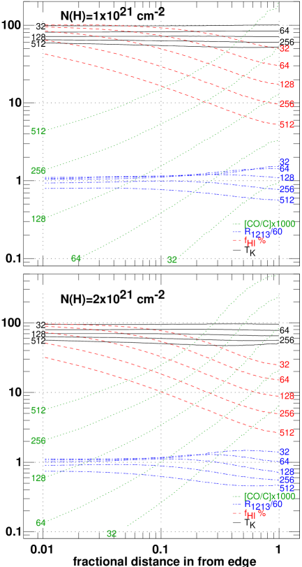
Figure 7: Radial variations in models with number densities n(H) = 32 .. 512 $~{}{\rm cm}^{-3}$ and front-back column densities N(H) $=1\times 10^{21}~{}{\rm cm}^{-2}$ (upper) and N(H) $=2\times 10^{21}~{}{\rm cm}^{-2}$ (lower). Shown are the kinetic temperture $T_{K}$ in black and solid; the percentage fraction of hydrogen in atomic form f_HI in red, dashed; n(CO)/n($\mathrm{{}^{13}CO}$) dash-dotted and blue; and $1000\times$ n(CO)/n(C⁺) in green and dotted.

References

- Bally & Langer (1982) Bally, J., & Langer, W. D. 1982, ApJ, 255, 143
- Bohlin et al. (1978) Bohlin, R. C., Savage, B. D., & Drake, J. F. 1978, ApJ, 224, 132
- Burgh et al. (2010) Burgh, E. B., France, K., & Jenkins, E. B. 2010, ApJ, 708, 334
- Burgh et al. (2007) Burgh, E. B., France, K., & McCandliss, S. R. 2007, ApJ, 658, 446
- Crenny & Federman (2004) Crenny, T., & Federman, S. R. 2004, ApJ, 605, 278
- Crutcher & Watson (1981) Crutcher, R. M., & Watson, W. D. 1981, ApJ, 244, 855
- Dame et al. (2001) Dame, T. M., Hartmann, D., & Thaddeus, P. 2001, ApJ, 547, 792
- Dickman (1978) Dickman, R. L. 1978, ApJS, 37, 407
- Draine (1978) Draine, B. T. 1978, ApJS, 36, 595
- Draine (2003) —. 2003, ARA&A, 41, 241
- Draine & Bertoldi (1996) Draine, B. T., & Bertoldi, F. 1996, ApJ, 468, 269
- Fukui et al. (2015) Fukui, Y., Torii, K., Onishi, T., et al. 2015, ApJ, 798, 6
- Gerin et al. (2016) Gerin, M., Neufeld, D. A., & Goicoechea, J. R. 2016, ARA&A, 54, 181
- Goldreich & Kwan (1974) Goldreich, P., & Kwan, J. 1974, ApJ, 189, 441
- Goldsmith (2013) Goldsmith, P. F. 2013, ApJ, 774, 134
- Goldsmith et al. (2008) Goldsmith, P. F., Heyer, M., Narayanan, G., et al. 2008, ApJ, 680, 428
- Grenier et al. (2005) Grenier, I. A., Casandjian, J.-M., & Terrier, R. 2005, Science, 307, 1292
- Gry et al. (2002) Gry, C., Boulanger, F., Nehmé, C., et al. 2002, A&A, 391, 675
- Heithausen (2006) Heithausen, A. 2006, A&A, 450, 193
- Hollenbach et al. (2012) Hollenbach, D., Kaufman, M. J., Neufeld, D., Wolfire, M., & Goicoechea, J. R. 2012, ApJ, 754, 105
- Indriolo et al. (2012) Indriolo, N., Neufeld, D. A., Gerin, M., et al. 2012, ApJ, 758, 83
- Indriolo et al. (2015) —. 2015, ApJ, 800, 40
- Jenkins & Tripp (2011) Jenkins, E. B., & Tripp, T. M. 2011, ApJ, 734, 65
- Kopp et al. (1996) Kopp, M., Gerin, M., Roueff, E., & Le Bourlot, J. 1996, A&A, 305, 558
- Lambert et al. (1994) Lambert, D. L., Sheffer, Y., Gilliland, R. L., & Federman, S. R. 1994, ApJ, 420, 756
- Lee et al. (1996) Lee, H. H., Herbst, E., Pineau Des Forets, G., Roueff, E., & Le Bourlot, J. 1996, A&A, 311, 690
- Leung & Liszt (1976) Leung, C.-M., & Liszt, H. S. 1976, ApJ, 208, 732
- Linke et al. (1977) Linke, R. A., Goldsmith, P. F., Wannier, P. G., Wilson, R. W., & Penzias, A. A. 1977, ApJ, 214, 50
- Liszt (2003) Liszt, H. 2003, A&A, 398, 621
- Liszt & Lucas (2002) Liszt, H., & Lucas, R. 2002, A&A, 391, 693
- Liszt (1984) Liszt, H. S. 1984, Comments on Astrophysics, 10, 137
- Liszt (1997) —. 1997, A&A, 322, 962
- Liszt (2007a) —. 2007a, A&A, 476, 291
- Liszt (2007b) —. 2007b, A&A, 461, 205
- Liszt (2008) —. 2008, A&A, 492, 743
- Liszt (2015) —. 2015, ApJ, 799, 66
- Liszt & Lucas (1998) Liszt, H. S., & Lucas, R. 1998, A&A, 339, 561
- Liszt & Pety (2012) Liszt, H. S., & Pety, J. 2012, A&A, 541, A58
- Liszt & Pety (2016) —. 2016, ApJ, 823, 124
- Liszt et al. (2010) Liszt, H. S., Pety, J., & Lucas, R. 2010, A&A, 518, A45
- Lucas & Liszt (1998) Lucas, R., & Liszt, H. 1998, A&A, 337, 246
- Lucas & Liszt (1996) Lucas, R., & Liszt, H. S. 1996, A&A, 307, 237
- McCall et al. (2002) McCall, B. J., Hinkle, K. H., Geballe, T. R., et al. 2002, ApJ, 567, 391
- Planck Collaboration et al. (2011) Planck Collaboration, Ade, P. A. R., Aghanim, N., et al. 2011, A&A, 536, A19
- Planck Collaboration et al. (2015) Planck Collaboration, Fermi Collaboration, Ade, P. A. R., et al. 2015, A&A, 582, A31
- Rachford et al. (2002) Rachford, B. L., Snow, T. P., Tumlinson, J., et al. 2002, ApJ, 577, 221
- Röllig & Ossenkopf (2013) Röllig, M., & Ossenkopf, V. 2013, A&A, 550, A56
- Roueff et al. (2015) Roueff, E., Loison, J. C., & Hickson, K. M. 2015, A&A, 576, A99
- Savage et al. (1977) Savage, B. D., Drake, J. F., Budich, W., & Bohlin, R. C. 1977, ApJ, 216, 291
- Sheffer et al. (2002) Sheffer, Y., Lambert, D. L., & Federman, S. R. 2002, ApJ, 574, L171
- Sheffer et al. (2008) Sheffer, Y., Rogers, M., Federman, S. R., et al. 2008, ApJ, 687, 1075
- Sheffer et al. (2007) Sheffer, Y., Rogers, M., Federman, S. R., Lambert, D. L., & Gredel, R. 2007, ApJ, 667, 1002
- Shepler et al. (2007) Shepler, B. C., Yang, B. H., Dhilip Kumar, T. J., et al. 2007, A&A, 475, L15
- Smith et al. (1978) Smith, A. M., Stecher, T. P., & Krishna Swamy, K. S. 1978, ApJ, 220, 138
- Smith & Adams (1980) Smith, D., & Adams, N. G. 1980, ApJ, 242, 424
- Sonnentrucker et al. (2007) Sonnentrucker, P., Welty, D. E., Thorburn, J. A., & York, D. G. 2007, ApJS, 168, 58
- Spitzer (1978) Spitzer, L. 1978, Physical processes in the interstellar medium (New York Wiley-Interscience, 1978. 333 p.)
- Stanimirović et al. (2014) Stanimirović, S., Murray, C. E., Lee, M.-Y., Heiles, C., & Miller, J. 2014, ApJ, 793, 132
- Sternberg et al. (2014) Sternberg, A., Le Petit, F., Roueff, E., & Le Bourlot, J. 2014, ApJ, 790, 10
- Szucs et al. (2014) Szucs, L., Glover, S. C. O., & Klessen, R. S. 2014, MNRAS, 445, 4055
- Szucs et al. (2016) —. 2016, MNRAS, 460, 82
- Van Dishoeck & Black (1988) Van Dishoeck, E. F., & Black, J. H. 1988, ApJ, 334, 771
- Visser et al. (2009) Visser, R., van Dishoeck, E. F., & Black, J. H. 2009, A&A, 503, 323
- Walker et al. (2015) Walker, K. M., Song, L., Yang, B. H., et al. 2015, ApJ, 811, 27
- Wannier et al. (1982) Wannier, P. G., Penzias, A. A., & Jenkins, E. B. 1982, ApJ, 254, 100
- Warin et al. (1996) Warin, S., Benayoun, J. J., & Viala, Y. P. 1996, A&A, 308, 535
- Watson et al. (1976) Watson, W. D., Anicich, V. G., & Huntress, W. T., J. 1976, ApJ, 205, L165
- Wilson et al. (1992) Wilson, T. L., Mauersberger, R., Langer, W. D., Glassgold, A. E., & Wilson, R. W. 1992, A&A, 262, 248
- Wolfire et al. (2010) Wolfire, M. G., Hollenbach, D., & McKee, C. F. 2010, ApJ, 716, 1191
- Wolfire et al. (2003) Wolfire, M. G., McKee, C. F., Hollenbach, D., & Tielens, A. G. G. M. 2003, ApJ, 587, 278