Meshfree elastoplastic solid for nonsmooth multidomain dynamics

Abstract

A method for simulation of elastoplastic solids in multibody systems with nonsmooth and multidomain dynamics is developed. The solid is discretised into pseudo-particles using the meshfree moving least squares method. The particles carry strain and stress tensor variables that are mapped to deformation constraints and constraint forces. The discretised solid model thus fit a unified framework for nonsmooth multidomain dynamics for realtime simulations including strong coupling of rigid multibodies with complex kinematic constraints such as articulation joints, unilateral contacts with dry friction, drivelines and hydraulics. The nonsmooth formulation allow for impulses, due to impacts for instance, to propagate instantly between the rigid multibody and the solid. Plasticity is introduced through an associative perfectly plastic modified Drucker-Prager model. The elastic and plastic dynamics is verified for simple test systems and the capability of simulating tracked terrain vehicles driving on a deformable terrain is demonstrated.

1 Introduction

We address the modeling and simulation of elastoplastic solids in multidomain environments including also mechatronic multibody systems with nonsmooth dynamics, such as vehicles, robots and processing machinery. Fast multidomain simulation is useful for concept design exploration, development of control algorithms and for interactive realtime simulators, e.g., for operator training, human-machine interaction studies and hardware-in-the-loop testing.

Realizing such simulators require integrating many subsystems of different types and complexity into a single multidomain dynamics model. If the subsystems are loosely coupled, the full system simulation can be realised by means of co-simulation [1], but this is not the general case. For the sake of computational performance, coarse grain models are often used, with rigid and flexible bodies coupled by kinematic constraints for modeling of joints and differential algebraic equation (dae) models for electronics, hydraulics and powertrain dynamics [2]. At coarse timescales the dynamics need to be treated as nonsmooth, allowing discontinuous velocities of rigid bodies undergoing impacts or frictional stick-slip transitions and instantaneous propagation of impulses through the system. This requires strong coupling through consistent mathematical formulation and coherent numerical treatment of the full system in order to achieve good stability and computational efficiency. Current techniques for co-simulation does not support that.

The theory and numerical methods for nonsmooth multidomain mechanics is covered in the reference [3]. The framework in [4, 5] is employed for constraint regularisation and stabilisation based on a discrete variational approach with constraints introduced as the stiff limit of energy and dissipation potentials.

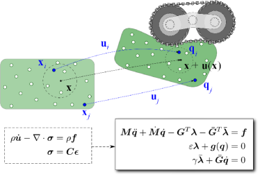
Figure 1: Illustration of the idea of using meshless discretisation and deformation constraints to obtain a unified multibody system model for both deformable solids and mechatronic systems.

The developed method is applicable to many different systems but one is primarily explored, namely the interaction between ground vehicles and deformable terrain [6]. Current solutions enable simulation of complex vehicle models with realtime performance but not including dynamic terrain models firmly based on solid mechanics in three dimensions. Usually, empirical terrain models of Bekker-Wong type are used [7, 8]. For more accurate offline simulations with fine temporal resolution, on the other hand, many solutions exist for elastoplastic solids coupled with tire models [9, 10] but scarcely with more complex multibody systems and not for realtime or faster simulation.

The main contribution in this paper, illustrated in figure 1, is a formulation and numerical method for simulation of elastoplastic solids as a nonsmooth multidomain multibody system on descriptor form [1]. This enables numerical integration with large timesteps that potentially exceed current solutions and provide realtime performance or better.

The regularisation and damping terms regulate the elasticity and viscous damping of deformations according to linear elasticity theory. An associative perfectly plastic Drucker-Prager model is employed using an elastic predictor-plastic corrector strategy to detect yielding and compute the plastic flow. In its basic form this model does not yield in hydrostatic compression in contrast to many real materials. Many soils yield under hydrostatic compression by failure in the microscopic structures whereby air and fluid is released. Therefore the Drucker-Prager model is extended to a capped version [12].

The dynamics of other subsystems and their potentially strong coupling is treated within the same multibody dynamics framework using a variational time integrator. Each timestep involve solving a block-sparse mixed linear complementarity problem mlcp, and can be efficiently integrated with tailored solvers.

A meshfree method [13, 14] is chosen in order to handle large deformations without need for remeshing [15] and, for future development, support fracturing and transitions to viscous flow or to granular media represented by contacting discrete elements. The displacement gradient and strain tensor is approximated by the method of moving least squares (mls) [16].

1.1 Notations

Matrices and vectors are represented in bold face in capital and lower case, $\bm{A}$ and $\bm{x}$, respectively. Latin superscripts indicate the index of a specific body $i,j,k=1,\ldots,N$, where $N$ is the total number of bodies in the system. Greek subscripts indicate a specific scalar component of a vector or matrix (may be multidimensional). The Einstein summation convention is used where repeated indices imply summation over them, e.g., representing matrix-vector multiplication as $\bm{A}\bm{x}=A_{\alpha\beta}x_{\beta}$. Subscripts $x,y$ or $z$ indicate a specific component of a vector or matrix assuming a Cartesian coordinate system. As an example of these notations the position vector of a body $i$ is denoted $\bm{q}^{i}$. The relative position of particle $j$ to $i$ is $\bm{q}^{ij}=\bm{q}^{j}-\bm{q}^{i}$. The $y$ component of this vector is $q^{ij}_{y}=q^{j}_{y}-q^{i}_{y}$. For rigid bodies, the position vector include also the rotation of the body. The system position vector is $\bm{q}=[\bm{q}^{1},\bm{q}^{2},\ldots,\bm{q}^{i},\ldots,\bm{q}^{N}]$. The gradient is denoted $\nabla_{\bm{x}}=\frac{\partial}{\partial\bm{x}}$ and $\nabla_{\alpha}=\frac{\partial}{\partial x_{\alpha}}$. The dot notation is used for the time derivative $\dot{}\equiv\tfrac{\text{d}}{\text{d}t}$.

2 Discrete multidomain dynamics

2.1 Lagrangian formulation

The Lagrangian of a constrained mechanical system is

$$\mathcal{L}(\bm{q},\dot{\bm{q}},\bm{\lambda},\bar{\bm{\lambda}}) =T(\bm{q},\dot{\bm{q}})-U(\bm{q})-\mathcal{R}(\bm{q},\dot{\bm{q}})$$

$$+\bm{\lambda}^{T}\bm{g}(\bm{q},t)+\bar{\bm{\lambda}}^{T}\bar{\bm{g}}(\bm{q},\dot{\bm{q}},t)$$ (1)

where $T(\bm{q},\dot{\bm{q}})=\tfrac{1}{2}\dot{\bm{q}}^{T}\bm{M}\dot{\bm{q}}$ is the kinetic energy, $U(\bm{q})$ is the potential energy and $\mathcal{R}(\bm{q},\dot{\bm{q}})$ is the Rayleigh dissipation function. The system state vector $(\bm{q},\dot{\bm{q}})$ is constrained by scleronomic holonomic constraints $0=\bm{g}(\bm{q})$, with Jacobian $\bm{G}=\partial\bm{g}/\partial\bm{q}$, and nonholonomic Pfaffian constraints $0=\bar{\bm{g}}(\bm{q},\dot{\bm{q}},t)\equiv\bar{\bm{G}}\dot{\bm{q}}-\bm{w}(t)$ with corresponding Lagrange multipliers $\bm{\lambda}$ and $\bar{\bm{\lambda}}$.

To ensure numerical stability it is common to regularise the constraints. This may be done by treating them as the limit of strong potentials and dissipation functions $U_{\varepsilon}(\bm{q})=\tfrac{1}{2\varepsilon}\bm{g}^{T}\bm{g}$ and $\mathcal{R}_{\gamma}(\bm{q},\dot{\bm{q}})=\tfrac{1}{2\gamma}\bar{\bm{g}}^{T}\bar{\bm{g}}$ with $\varepsilon,\gamma\to 0$ [17]. In fact, any stiff force can be transformed into a regularised constraint through a Legendre transform [5]

$$U_{\varepsilon}(\bm{q}) =\bm{\lambda}^{T}\bm{g}-\tfrac{\varepsilon}{2}\bm{\lambda}^{T}\bm{\lambda}$$ (2)

$$\mathcal{R}_{\gamma}(\bm{q},\dot{\bm{q}}) =\bar{\bm{\lambda}}^{T}\bar{\bm{g}}-\tfrac{\gamma}{2}\bar{\bm{\lambda}}^{T}\bar{\bm{\lambda}}$$ (3)

This transform the Euler-Lagrange equations of motion into

$$\bm{M}\ddot{\bm{q}}+\dot{\bm{M}}\dot{\bm{q}}-\bm{G}(\bm{q})^{T}\bm{\lambda}-\bar{\bm{G}}(\bm{q})^{T}\bar{\bm{\lambda}} =\bm{f}$$ (4)

$$\varepsilon\bm{\lambda}+\bm{g}(\bm{q}) =0$$ (5)

$$\gamma\bar{\bm{\lambda}}+\bar{\bm{G}}(\bm{q})\dot{\bm{q}} =\bm{w}(t)$$ (6)

where $\bm{f}\equiv-\nabla_{\bm{q}}U(\bm{q})-\nabla_{\dot{\bm{q}}}\mathcal{R}(\bm{q},\dot{\bm{q}})$ are the explicit forces from weak smooth potentials. This constitute a system of dae of index 1, which are easier to integrate numerically than the corresponding higher index dae in the absence of regularisation and stabilisation. $\varepsilon=\gamma=0$. A term for dissipation of motion orthogonal to the holonomic constraint surface can be added to improve the convergence. Also this dissipation can be physically based by introducing it as a Legendre transform of a Rayleigh dissipation function $\mathcal{R}_{\tau}(\bm{q},\dot{\bm{q}})=\tfrac{\tau}{2\varepsilon}\dot{\bm{g}}^{T}\dot{\bm{g}}\to\tau\dot{\bm{\lambda}}^{T}\dot{\bm{g}}-\tfrac{\tau\varepsilon}{2}\dot{\bm{\lambda}}^{T}\dot{\bm{\lambda}}$, with damping parameter $\tau$. This modifies Eq. (5) to

$$\varepsilon\bm{\lambda}+\varepsilon\tau\dot{\bm{\lambda}}+\bm{g}(\bm{q})+\tau\bm{G}\dot{\bm{q}}=0$$ (7)

The compliance and damping factors $\varepsilon$, $\tau$ and $\gamma$ are not restricted to being scalar or diagonal. In what follows these are assumed to be matrices.

2.2 Time discretisation

Variational integration [18] provides a systematic approach to derive time integration schemes with good properties, e.g., momentum preservation and symplecticity. Rather than discretising the Euler-Lagrange equations of motion directly, the Lagrangian and principle of least action is defined in time-discrete form. Employing semi-implicit Euler discretisation and linearising the constraint as $\bm{g}(\bm{q}+\Delta\bm{q})=\bm{g}(\bm{q})+\bm{G}\Delta\bm{q}$ leads to the following scheme

$$\bm{q}_{n+1} =\bm{q}_{n}+h\dot{\bm{q}}_{n+1}$$ (8)

$$\begin{bmatrix}\bm{M}&-\bm{G}^{T}&-\bar{\bm{G}}^{T}\\ \bm{G}&\bm{\Sigma}&0\\ \bar{\bm{G}}&0&\bar{\bm{\Sigma}}\end{bmatrix}\begin{bmatrix}\dot{\bm{q}}_{n+1}\\ \bm{\lambda}\\ \bar{\bm{\lambda}}\end{bmatrix}=\begin{bmatrix}\bm{p}_{n}\\ \bm{v}_{n}\\ \bm{\omega}_{n}\end{bmatrix}$$ (9)

where $\bm{p}_{n}=M\dot{\bm{q}}_{n}+h\bm{f}_{n}$, $\bm{v}_{n}=-\frac{4}{h}\Upsilon g+\Upsilon G\dot{\bm{q}}_{n}$ and regularisation and stabilisation matrices $\bm{\Sigma}=\text{diag}(4\varepsilon/h^{2}(1+4\tau/h))$, $\bar{\bm{\Sigma}}=\text{diag}(\gamma/h)$ and $\bm{\Upsilon}=\text{diag}(1+4\tau/h)^{-1})$. Eq. (9) is a linear system of $N=\dim(\dot{\bm{q}})+\dim(\bm{g})+\dim(\bar{\bm{g}})$ equations. The matrix on the left hand side is block-sparse, positive definite and non-symmetric. The regularisation appearing as the diagonal perturbation matrices $\bm{\Sigma}$ and $\bar{\bm{\Sigma}}$ are needed for handling otherwise ill-posed or ill-conditioned problems, e.g., systems with constraint degeneracy and large mass ratios. The stabilisation terms $-\frac{4}{h}\Upsilon g+\Upsilon G\dot{\bm{q}}_{n}$ on the right hand side counteract constraint violations, e.g., sudden and large contact penetrations at impacts or small numerical constraint drift. The presented stepping scheme, referred to as spook, has been proved to be linearly stable [4] and numerical simulations suggest a large domain of nonlinear stability.

The combined effect of the regularisation and stabilisation terms is to bring elastic and viscous properties to motion orthogonal to the constraint surface $\bm{g}(\bm{q})=0$, e.g., for modeling elasticity in mechanical joints. The parameters $\varepsilon$ and $\gamma$ need not be chosen arbitrarily, as for the conventional approaches to constraint regularisation and stabilisation, but can be based on physics models using parameters that can be derived from first principles, found in literature or be identified by experiments. This becomes straightforward when the regularisation is introduced by potential energy as quadratic functions in $\bm{g}$, i.e., $U_{\varepsilon}(\bm{q})=\tfrac{1}{2}\bm{g}^{T}\bm{\varepsilon}^{-1}\bm{g}$. This has been exploited in previous work to constraint based modeling of lumped element beams [19], wires [20], meshfree fluids [21] and granular material [22].

2.3 nonsmooth dynamics

In discrete time, some of the dynamics is best treated as nonsmooth [3], meaning that the velocity may change discontinuously to fulfil inequality constraints and complementarity conditions. Introducing such conditions is an efficient way of modeling contacts, dry friction, joint limits, electric circuit switching, motor and actuator dynamics and control systems for discrete time with large step size. The alternative would be to use a fine enough temporal resolution where the dynamics appear smooth and may be modeled by daes or ordinary differential equations alone. In general, this is an intractable approach for full system simulations and interactive applications. The nonsmooth dynamics can be formally treated as differential variational inequalities [23]. The discrete equations of motion (9) take the form of a mixed linear complementarity problem, mlcp, when nonsmooth dynamics is included

$$\bm{H}\bm{z}+\bm{r} =\bm{w}_{+}-\bm{w}_{-}$$ (10)

$$0\leq\bm{w}_{+} \perp\bm{z}-\bm{l}\geq 0$$

$$0\leq\bm{w}_{-} \perp\bm{u}-\bm{z}\geq 0$$

where $\bm{H}\bm{z}$ corresponds to the left hand side of equation (9), $\bm{r}$ is the negated right hand side and $\bm{w}_{\pm}$ are slack variables. The terms $\bm{u}$ and $\bm{l}$ correspond to the upper and lower limits on the solution vector $\bm{z}$, respectively. The original linear system of equations is recovered by assigning $\pm\infty$ to the upper and lower limits, i.e., no limit.

Rigid body contacts are handled by the Signorini-Coulomb law for unilateral dry frictional contacts. This states that if the non-penetration constraint, $g\geq 0$, is violated then the normal contact velocity and constraint force are complementary in ensuring separation, $0\leq{v}_{\text{n}}\perp{\lambda}_{\text{n}}\geq 0$, and the tangential friction force, acting to maintain zero slip, is bound to be on or inside the Coulomb friction cone, $|{\bm{\lambda}}_{\text{t}}|\leq\mu{\lambda}_{\text{n}}$. The latter may be linearised by approximating the cone with a polyhedral or a box. Impacts are treated post facto in a separate impact stage succeeding the update of velocities and positions. At the impact stage an impulse transfer is applied enabling discontinuous velocity changes, i.e., from $\dot{\bm{q}}^{−}$ to $\dot{\bm{q}}^{+}$. Newtons’ impact law, $\bm{n}^{T}\dot{\bm{q}}^{+}=-e\bm{n}^{T}\dot{\bm{q}}^{-}$, is used with restitution coefficient $e$ in conjunction with preserving all other constraints, $\bm{G}\dot{\bm{q}}=0$. This amounts to solving the same mlcp (10) but with $h\bm{f}_{n}=\bm{0}$ and $-\frac{4}{h}\Upsilon g+\Upsilon G\dot{\bm{q}}_{n}=\bm{0}$ in the right hand side of equation (9).

A fixed timestep approach is preferred when aiming for fast full systems simulations with many nonsmooth events with inequality or complementarity conditions, e.g., involving thousands or millions of dynamic contacts, switching in electric, hydraulic or control systems, or elastic material undergoing fracture or plastic failure. Using variable timestep and exact event location become computationally intractable and may fail by occurrence of Zeno points.

2.4 Heterogeneous multidomain dynamics

In a multidomain simulation with strongly coupled subsystems the nonsmooth dynamics propagate instantly throughout the full system. The dynamics in the elastoplastic solid may be directly and strongly coupled with the internal dynamics of a mechatronical system. The nonsmooth multidomain dynamics approach with physics based constraint regularisation and stabilisation presented here, provides a general framework for building and efficiently solving the dynamics on mlcp form. Each subsystem take the same generic form of saddle-point matrix as the full system in Eq. (9). Considering a system with two subsystems $A$ and $B$, the full coupled system takes the following form

$$\bm{H}\bm{z} =\begin{bmatrix}[cc|c]\bm{H}_{A}&0&-\bm{G}^{T}_{{AB}_{A}}\\ 0&\bm{H}_{B}&-\bm{G}^{T}_{{AB}_{B}}\\ \hline\cr\bm{G}_{{AB}_{A}}&\bm{G}_{{AB}_{B}}&\bm{\Sigma}_{AB}\end{bmatrix}\begin{bmatrix}\bm{z}_{A}\\ \bm{z}_{B}\\ \bm{\lambda}_{AB}\end{bmatrix}$$ (11)

where $\bm{\lambda}_{AB},[\bm{G}_{{AB}_{A}},\bm{G}_{{AB}_{B}}],\bm{\Sigma}_{AB}$ are the multiplier, Jacobian and regularisation of the subsystem coupling.

3 Constraint based meshfree elastoplastic solid

3.1 Elastoplastic solid

The solid is assumed to sustain geometric large deformations. The St. Venant-Kirchoff elasticity model is used in combination with the Drucker-Prager plasticity model [11]. The material strain is expressed by the Green-Lagrange strain tensor

$$\epsilon_{\alpha\beta}(\bm{x}) =\frac{1}{2}\left(\nabla_{\alpha}u_{\beta}+\nabla_{\beta}u_{\alpha}+\nabla_{\alpha}u_{\gamma}\nabla_{\beta}u_{\gamma}\right)$$ (12)

where $\bm{u}(\bm{x})$ is the displacement field mapping a reference coordinate $\bm{x}$ to displaced position $\tilde{\bm{x}}(\bm{x})=\bm{x}+\bm{u}(\bm{x})$. Observe that the Green-Lagrange strain tensor transforms under large rotations and no co-rotation procedure is needed. It is convenient to use the Voigt notation for representing the strain tensor on vector format, $\bm{\epsilon}=\left[\epsilon_{xx},\epsilon_{yy},\epsilon_{zz},2\epsilon_{yz},2\epsilon_{xz},2\epsilon_{xy}\right]^{T}$, and the stress tensor $\bm{\sigma}=\left[\sigma_{xx},\sigma_{yy},\sigma_{zz},\sigma_{yz},\sigma_{xz},\sigma_{xy}\right]^{T}$ such that the linear constitutive law reads $\bm{\sigma}=\bm{C}\bm{\epsilon}$, with stiffness matrix

$$\bm{C}=\begin{bmatrix}\lambda+2\mu&\lambda&\lambda&0&0&0\\ \lambda&\lambda+2\mu&\lambda&0&0&0\\ \lambda&\lambda&\lambda+2\mu&0&0&0\\ 0&0&0&\mu&0&0\\ 0&0&0&0&\mu&0\\ 0&0&0&0&0&\mu\end{bmatrix}$$ (13)

where $\lambda$ and $\mu$ are the first and second Lamé parameters which are related to the Young’s modulus and Poisson’s ratio, $E$ and $\nu$, of a material as $\lambda=E\nu/\left(1+\nu\right)\left(1-2\nu\right)$ and $\mu=E/2\left(1+\nu\right)$. The corresponding strain energy density is

$$U(\bm{x})=\frac{1}{2}\bm{\epsilon}^{T}\bm{C}\bm{\epsilon}=\lambda(\operatorname{tr}\bm{\epsilon})^{2}+2\mu\operatorname{tr}(\bm{\epsilon}^{2})$$ (14)

Plastic deformation occur when the stress of a material reaches its yield strength, $\Phi(\bm{\sigma})=0$, in which case the material undergo plastic flow if the load is increased further. The choice of yield function, $\Phi(\bm{\sigma})$, is based on the type of material being modeled. To represent the permanent plastic deformation, the strain tensor is decomposed into an elastic and a plastic component, $\bm{\epsilon}=\bm{\epsilon}^{\text{e}}+\bm{\epsilon}^{\text{p}}$. In ideal plasticity the plastic deformation occurs instantly according to a flow rule $\text{d}\bm{\epsilon}^{\text{p}}=\text{d}\bm{\lambda}^{\text{p}}\frac{\partial\Psi}{\partial\bm{\sigma}}$, where $\Psi(\bm{\sigma})$ is the plastic potential and $\bm{\lambda}^{\text{p}}$ is the plastic multiplier. If $\Psi(\bm{\sigma})=\Phi(\bm{\sigma})$ the model is said to be associative and otherwise non-associative. The plastic flow last as long as it is positive, $\text{d}\bm{\lambda}^{\text{p}}>0$, incrementally reducing the stress $\text{d}\bm{\sigma}^{\text{p}}$, until it reaches the elastic regime, $\Phi(\sigma)<0$. This constitute a nonlinear complementarity problem known as Karush-Kuhn-Tucker conditions

$$\Phi\leq 0,\;\;\text{d}\bm{\lambda}^{\text{p}}\geq 0,\;\;\Phi\ \text{d}\bm{\lambda}^{\text{p}}=0$$ (15)

The plastic multiplier is computed from the constitutive law, which in the plastic flow phase is $\text{d}\bm{\sigma}={\bm{C}}^{\text{p}}\text{d}\bm{\epsilon}$, where the elastoplastic tangent stiffness matrix is

$${\bm{C}}^{\text{p}}=\bm{C}-\frac{\bm{C}\frac{\partial\Psi}{\partial\bm{\sigma}}(\frac{\partial\Phi}{\partial\bm{\sigma}})^{T}\bm{C}}{(\frac{\partial\Phi}{\partial\bm{\sigma}})^{T}\bm{C}\frac{\partial\Psi}{\partial\bm{\sigma}}}$$ (16)

Predictor-corrector algorithms are conventionally used to integrate the plastic flow. In the absence of plastic hardening or softening, the plastic deformation, plastic multiplier and total stress can be computed easily using the radial return algorithm [11] summarised in Algorithm 2.

The assumed plasticity model is a capped Drucker-Prager model, following Dolarevic [12], with a compaction variable $\kappa$. The yield function $\Phi\left(\bm{\sigma},\kappa\right)$ is a piecewise function consisting of the Drucker-Prager, tension and compression cap functions according to (17)

$$\Phi\left(\bm{\sigma},\kappa\right)=\begin{cases}\Phi_{\textsc{\tiny T}}\left(I_{1},J_{2}\right)&I_{1}\geq I_{1}^{\textsc{\tiny T}}\\ \Phi_{\textsc{\tiny DP}}\left(I_{1},J_{2}\right)&I_{1}^{\textsc{\tiny T}}>I_{1}>I_{1}^{\textsc{\tiny C}}\left(\kappa\right)\\ \Phi_{\textsc{\tiny C}}\left(I_{1},J_{2},\kappa\right)&I_{1}^{\textsc{\tiny C}}\left(\kappa\right)\geq I_{1}\end{cases}$$ (17)

where $I_{1}=\operatorname{tr}(\bm{\sigma})$ is the first invariant of the stress tensor and $J_{2}=0.5\operatorname{tr}(\bar{\bm{\sigma}}^{2})$ is the second invariant of the deviatoric stress tensor $\bar{\bm{\sigma}}=\bm{\sigma}-\tfrac{1}{3}I_{1}\bm{1}$. The expressions for the tension cap $\Phi_{\textsc{\tiny T}}\left(I_{1},J_{2}\right)$ and compression cap $\Phi_{\textsc{\tiny C}}\left(I_{1},J_{2},\kappa\right)$ are given in Appendix A and the Drucker-Prager surface is defined as

$$\Phi_{\textsc{\tiny DP}}\left(I_{1},J_{2}\right)=\sqrt{J_{2}}+\frac{\eta}{3}I_{1}-\xi c$$ (18)

where $\phi$ is the internal friction angle and $c$ the cohesion parameter such that $\eta=6\sin\phi/\sqrt{3}\left(3-\sin\phi\right)$ and $\xi=6\cos\phi/\sqrt{3}\left(3-\sin\phi\right)$.

The capped yield surface is illustrated in Figure 2. The tension cap is fix and is used to regularise the plastic flow behaviour in the corner region. The compression surface cap, on the other hand, is dynamic and the maximum hydrostatic pressure, $\kappa$, is used as main variable.

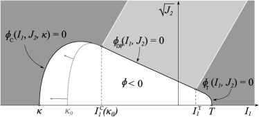
Figure 2: The capped Drucker-Prager yield surface. The non-shaded region indicate the elastic domain, which grows under plastic compression.

The conventional Drucker-Prager model is a common model for the plastic deformation dynamics of soils, e.g. wet or dry sand. These materials are weak under tensile stress ($I_{1}>0$) and become stronger under compression ($I_{1}<0$) where it may support large shear stresses ($\sqrt{J_{2}}$). The capped Drucker-Prager model is a generalisation that include also plastic compaction that may occur in many soils. The compaction mechanism may be failure of the individual grains whereby air or water is displaced from the soil. The compaction saturates at a maximum level, where all voids are vanished. The compaction dynamics is modeled by a variable cap on compressive side of the Drucker-Prager yield surface, intersecting the hydrostatic axis at $-\kappa$. The compaction hardening law is chosen

$$\kappa=\kappa_{0}+\frac{1}{D}\ln\left(1+\frac{\operatorname{tr}({\bm{\epsilon}}^{\text{p}})}{W}\right)$$ (19)

where $W$ is the maximum volume compaction, $D$ is the hardening rate and $\kappa_{0}$ the initial cap position where compressive failure first occur. Observe that when the plastic volume compaction $-\operatorname{tr}({\bm{\epsilon}}^{\text{p}})$ approaches $W$, the cap variable $\kappa$ goes to infinity, the material does not compact further plastically and behave like the standard Drucker-Prager model. The elastoplastic material parameters are summarised in Table 1. Expressions for the detailed shape of the compression cap and the derivatives of the yield functions are found in Appendix A.

Table 1: Elastoplastic model parameters

$E,\nu$	Young’s modulus and Poisson’s ratio
$\phi,c$	friction angle and cohesion
$W,D$	max compaction and hardening rate
$T,\kappa$	Cap $I_{1}$-intersections

3.2 Meshfree method

The continuous solid of mass $m$ and reference volume $V$ is discretised into ${N}_{\text{p}}$ particles. The particles have mass $m^{i}=m/{N}_{\text{p}}$, volume $V^{i}=V/{N}_{\text{p}}$, position $\bm{q}^{i}$ and velocity $\dot{\bm{q}}^{i}$. The particle displacement is $\bm{u}^{i}=\bm{q}^{i}-\bm{x}^{i}$ with reference position $\bm{x}^{i}$ as illustrated in figure 1. A continuous and differentiable displacement field is approximated using the mls method [16, 24]. The differentiated displacement field defines the strain tensor field in any point as described in equation (12). The particles can thus be understood as pseudo-particles having both particle and field properties.

The mls approximation of the displacement field is

$$u_{\alpha}(\bm{x})=\sum_{j}^{{N}_{\text{p}}}\Psi_{j}(\bm{x})u^{j}_{\alpha}$$ (20)

where the shape function and moment matrix use a quadratic basis

$$\Psi_{j}(\bm{x}) =p_{\gamma}(\bm{x})A_{\gamma\tau}^{-1}(\bm{x})p_{\tau}(\bm{x}^{j})W\left(\bm{x}-\bm{x}^{j}\right)$$

$$A_{\gamma\tau}(\bm{x}) =\sum_{j}^{{N}_{\text{p}}}W\left(\bm{x}-\bm{x}^{j}\right)p_{\gamma}^{j}p_{\tau}^{j}$$ (21)

$$\bm{p}(\bm{x}) =\left[1,\ x,\ y,\ z,\ yz,\ xz,\ xy,\ x^{2},\ y^{2},\ z^{2}\right]^{T}\textasciiacute$$

and weight function $W(\bm{x})=\frac{315}{64\pi l^{9}}(l^{2}-\bm{x}^{T}\bm{x})^{3}$ if $|\bm{x}|$is smaller than the influence radius $l$, and otherwise zero. The base function notation $\bm{p}^{j}=\bm{p}(\bm{x}^{j})$ is used to simplify the expressions. The gradient of the interpolated displacement field is

$$\nabla_{\beta}u_{\alpha}(\bm{x}) =\sum_{j}^{{N}_{\text{p}}}\nabla_{\beta}\Psi_{j}(\bm{x})u^{j}_{\alpha}$$ (22)

$$\nabla_{\beta}\Psi_{j}= \nabla_{\beta}p_{\gamma}{A}_{\gamma\tau}^{-1}p^{j}_{\tau}W^{j}+p_{\gamma}\nabla_{\beta}{A}_{\gamma\tau}^{-1}p^{j}_{\tau}W^{j}$$

$$+p_{\gamma}{A}_{\gamma\tau}^{-1}p^{j}_{\tau}\nabla_{\beta}W^{j}$$ (23)

with $W^{j}=W(\bm{x}-\bm{x}^{j})$, $\nabla_{\beta}W^{j}=\nabla_{x_{\beta}}W(\bm{x}-\bm{x}^{j})$. The strain tensor field, $\bm{\epsilon}(\bm{x})$, can thus be approximated by applying Eq. (22) to Eq. ((12)). Observe that $u^{j}_{\alpha}$ depend on current particle positions $\bm{q}$ while $\nabla_{\beta}\Psi_{j}(\bm{x})$ depend only on the reference positions.

3.3 Deformation constraint

The strain energy density, $U(\bm{x})=\tfrac{1}{2}\bm{\epsilon}^{T}\bm{C}\bm{\epsilon}$, is transformed into a regularised constraint via a Legendre transform as presented in Sec. (2). For each particle a deformation constraint is imposed

$$\bm{g}^{i}=\begin{bmatrix}[c]\epsilon^{i}_{xx}\\ \epsilon^{i}_{yy}\\ \epsilon^{i}_{zz}\\ \epsilon^{i}_{yz}+\epsilon^{i}_{zy}\\ \epsilon^{i}_{zx}+\epsilon^{i}_{xz}\\ \epsilon^{i}_{xy}+\epsilon^{i}_{yx}\end{bmatrix}$$ (24)

with particle strain components $\epsilon^{i}_{\alpha\beta}=\frac{1}{2}(s^{i}_{\alpha\beta}+s^{i}_{\beta\alpha}+s^{i}_{\gamma\alpha}s^{i}_{\gamma\beta})$ based on the displacement gradient $s^{i}_{\alpha\beta}(\bm{q})=\nabla_{\beta}u_{\alpha}(\bm{x}^{i},\bm{q})$ for particle $i$, computed by evaluating the field at $\bm{x}=\bm{x}^{i}$. The compliance parameter become $\bm{\varepsilon}^{i}=(V^{i}\bm{C}^{i})^{-1}$. Observe that the compliance depend only on the material parameters, through Eq. ((13)), and on the spatial resolution through the particle volume factor $V^{i}$ that appear when integrating from energy density to particle energy.

The Jacobian of the deformation constraint, $\bm{G}=\partial\bm{g}/\partial\bm{q}$ , can be expanded through the chain rule to

$$G^{i}_{\alpha\beta}(\bm{q})=\frac{\partial g^{i}_{\alpha}}{\partial\epsilon^{i}_{\gamma\eta}}\frac{\partial\epsilon^{i}_{\gamma\eta}}{\partial s^{i}_{\tau\kappa}}\frac{\partial s^{i}_{\tau\kappa}}{\partial q_{\beta}^{j}}$$ (25)

The Jacobian for constraint $i$ has block structure $\bm{G}^{i}=[\bm{G}^{i1},\ldots,\bm{G}^{ij},\ldots,\bm{G}^{i{N}_{\text{p}}}]$, where each block element $\bm{G}^{ij}$ has dimension $6\times 3$. For notational convenience the constraint vector is split in two parts, one for the diagonal terms of the strain tensor, ${\bm{g}}_{\text{d}}^{i}=[\epsilon^{i}_{xx},\epsilon^{i}_{yy},\epsilon^{i}_{zz}]^{T}$ and one for the off-diagonal terms ${\bm{g}}_{\text{od}}^{i}=[\epsilon^{i}_{yz}+\epsilon^{i}_{zy},\ \epsilon^{i}_{zx}+\epsilon^{i}_{xz},\ \epsilon^{i}_{xy}+\epsilon^{i}_{yx}]^{T}$. The Jacobian blocks $\bm{G}^{ij}$ are splitted correspondingly in two $3\times 3$ Jacobian blocks, $\bm{G}^{ij}=[{{\bm{G}}_{\text{d}}^{ij}}^{T},\ {{\bm{G}}_{\text{od}}^{ij}}^{T}]^{T}$. After some lengthy algebra the following expressions for the Jacobians are found

$${\bm{G}}_{\text{d}}^{ij} =\begin{bmatrix}(1+s^{i}_{xx})\Lambda^{ij}_{x}&s^{i}_{yx}\Lambda^{ij}_{x}&s^{i}_{zx}\Lambda^{ij}_{x}\\ s^{i}_{xy}\Lambda^{ij}_{y}&(1+s^{i}_{yy})\Lambda^{ij}_{y}&s^{i}_{zy}\Lambda^{ij}_{y}\\ s^{i}_{xz}\Lambda^{ij}_{z}&s^{i}_{yz}\Lambda^{ij}_{z}&(1+s^{i}_{zz})\Lambda^{ij}_{z}\end{bmatrix}$$ (26)

$${\bm{G}}_{\text{od}}^{ij} =\begin{bmatrix}s^{i}_{xy}\Lambda^{ij}_{z}+s^{i}_{xz}\Lambda^{ij}_{y}\;&(1+s^{i}_{yy})\Lambda^{ij}_{z}+s^{i}_{yz}\Lambda^{ij}_{y}\;&s^{i}_{zy}\Lambda^{ij}_{z}+(1+s^{i}_{zz})\Lambda^{ij}_{y}\\ s^{i}_{xz}\Lambda^{ij}_{x}+(1+s^{i}_{xx})\Lambda^{ij}_{z}\;&s^{i}_{yz}\Lambda^{ij}_{x}+s^{i}_{yx}\Lambda^{ij}_{z}\;&(1+s^{i}_{zz})\Lambda^{j}_{x}+s^{i}_{zx}\Lambda^{j}_{z}\\ (1+s^{i}_{xx})\Lambda^{ij}_{y}+s^{i}_{xy}\Lambda^{ij}_{x}\;&s^{i}_{yx}\Lambda^{ij}_{y}+(1+s^{i}_{yy})\Lambda^{ij}_{x}\;&s^{i}_{zx}\Lambda^{ij}_{y}+s^{i}_{zy}\Lambda^{ij}_{x}\end{bmatrix}$$ (27)

where $\Lambda^{ij}_{\beta}=\nabla_{\beta}\Psi_{j}(\bm{x}^{i})$. Observe that only $s^{i}_{\alpha\beta}(\bm{q})$ depend on the current particle positions while $\Lambda^{ij}_{\beta}$ only depend on the reference positions and may thus be precomputed. In the derivation of the Jacobians the following partial derivatives are used

$$\frac{\partial\epsilon^{i}_{\gamma\eta}}{\partial s^{i}_{\tau\kappa}}= \tfrac{1}{2}(\delta_{\gamma\tau}^{\eta\kappa}+\delta_{\eta\tau}^{\gamma\kappa}+\delta_{\kappa\gamma}\nabla\bm{u}^{i}_{\tau\eta}+\delta_{\eta\kappa}\nabla\bm{u}^{i}_{\tau\gamma})$$

$$\frac{\partial s^{i}_{\tau\kappa}}{\partial q_{\beta}^{j}}= \delta_{\tau\beta}\nabla_{\kappa}\Psi_{j}(\bm{x}^{i})$$

with Kronecker notation $\delta_{\gamma\tau}^{\eta\kappa}\equiv\delta_{\gamma\tau}\delta_{\eta\kappa}$.

4 Simulation

The procedure, implementation details and results for nonsmooth multidomain dynamic simulation including elastoplastic solids is presented in this section. The main simulation algorithm is given in section 4.1. The elastoplastic solid model is implemented in C++ as an extension to the simulation software AgX Dynamics [25] making use of its data types, collision detection algorithms and solver framework, which support simulation of nonsmooth rigid multibody dynamics systems in the formulation of section 2. The mlcp solver framework is covered in section 4.2. The elastic and plastic model and implementation is verified by performing load-displacement simulation tests presented in section 4.3. Finally, in section 4.4, the applicability of the approach is demonstrated by multidomain examples including a simple terrain vehicle with tracked bogies driving over a deformable terrain and simulated cone penetrometer test in soil with embedded rock.

4.1 Main algorithm

Algorithm 1 lists the main steps in running a multidomain dynamics simulation including both elastoplastic solids and contacting rigid multibodies.

Algorithm 1 Main simulation algorithm

1:  initialisation of bodies and constraints

2:  compute mlcp blocks $\bm{M},\bm{\Sigma},\bm{\Upsilon}$

3:  compute mls blocks $\bm{A}^{-1}_{i}$, $\bm{\Lambda}_{i}$

4:  for all timestep $n=1,2,\ldots$ do

5:     get input signals and explicit forces

6:     do contact detection

7:     for all particles $i=1,2,\ldots{N}_{\text{p}}$ do

8:        compute $\bm{u}^{i}_{n}$ and $\bm{\epsilon}^{i}_{n}={\bm{J}^{i}_{n}}^{T}\bm{J}^{i}_{n}-\bm{1}$

9:        $[\bm{\epsilon}^{\text{e},i}_{n},\bm{\epsilon}^{\text{p},i}_{n}]=\mathrm{radial\_return}(\bm{\epsilon}^{i}_{n},\bm{\epsilon}^{\text{p},i}_{n-1})$

10:     end for

11:     compute constraint data $\bm{G},\bm{g}$

12:     build mlcp data $\bm{H},\bm{r},\bm{l},\bm{u}$

13:     solve $\bm{z}=$ mlcp($\bm{H},\bm{r},\bm{l},\bm{u}$)

14:     get $\dot{\bm{q}}_{n+1}$ and constraint force $\bm{G}^{T}\bm{\lambda}$

15:     update position $\bm{q}_{n+1}=\bm{q}_{n}+h\dot{\bm{q}}_{n+1}$

16:     store and visualise the new state

17:  end for

18:  post-process and visualise stored data

Algorithm 2 Plastic radial return algorithm

1:  input total strain $\bm{\epsilon}_{n}$ and stored plastic $\bm{\epsilon}^{\text{p}}_{n-1}$

2:  trial plastic strain $\bm{\epsilon}^{\text{p}}_{n}=\bm{\epsilon}^{\text{p}}_{n-1}$

3:  compute trial stress $\bm{\sigma}_{n}=\bm{C}(\bm{\epsilon}_{n}-\bm{\epsilon}_{n}^{\text{p}})$

4:  if yielding $\Phi(\bm{\sigma}_{n})>0$ then

5:     return to surface

6:     while $\left|\Phi(\bm{\sigma}_{n})\right|>{\varepsilon}_{\text{tol}}$ do

7:        $\Delta\bm{\lambda}=\frac{\Phi(\bm{\sigma}_{n})}{\frac{\partial\Phi}{\partial\bm{\sigma}}{\bm{C}}_{\text{}}\frac{\partial\Psi}{\partial\bm{\sigma}}}$

8:        $\Delta\bm{\epsilon}^{\text{p}}=\Delta\bm{\lambda}\frac{\partial\Psi}{\partial\bm{\sigma}}$

9:        $\Delta\bm{\sigma}=\Delta\bm{\lambda}\bm{C}\frac{\partial\Psi}{\partial\bm{\sigma}}$

10:        $\bm{\epsilon}^{\text{p}}_{n}=\bm{\epsilon}^{\text{p}}_{n}+\Delta\bm{\epsilon}^{\text{p}}$

11:        $\bm{\sigma}_{n}=\bm{\sigma}_{n}-\Delta\bm{\sigma}$

12:     end while

13:     update cap variables $\kappa_{n}(\bm{\epsilon}^{\text{p}})$ and ${I_{1}^{c}}_{n}(\bm{\sigma}_{n})$

14:  end if

15:  compute elastic strain $\bm{\epsilon}^{\text{e}}_{n}=\bm{C}^{-1}\bm{\sigma}_{n}$

If the trial stress is outside the elastic domain the radial return algorithm 2 return the system radially to the nearest point on the yield surface, either to the Drucker-Prager surface, or to the tension or compression cap, see Fig. 2. After returning the stress to the yield surface, with an error threshold ${\varepsilon}_{\text{tol}}$, the compaction variable $\kappa$ is updated.

The elastoplastic solid is initialised by defining a solid volume and assigning material parameters. The solid is discretised into ${N}_{\text{p}}$ pseudo-particles according to a given spatial resolution. For simplicity, the particles are positioned in a regular cubic grid. This defines the reference state with vanishing strain and stress. Any initial displacement may be applied to the particles. The elastoplastic constraints are initialised and connectivity data listing the particles involved in each constraint. Similarly, rigid bodies and kinematic constraints are defined, for instance, to form an articulated vehicle and powertrain. Each body is assigned a geometric 3D shape. Contact properties are assigned to each body, including coefficient of restitution, elasticity and friction. These are used to generate contact constraint data included in the mlcp when triggered by contact detection algorithm. The pseudo-particles are given a spherical geometric shape for dynamic contacts with rigid bodies and static geometries. Fixed-point or plane constraints can also be defined to model permanent boundary conditions. Contacts between particles are disabled. Certain quantities are computed once before time integration and then reused for the sake of optimisation, e.g., the inverse moment matrix $\bm{A}^{-1}$ in the mls approximation, $\nabla_{\beta}\Phi$ and $\bm{\Lambda}$.

The simulation is run with fixed timestep, following the stepper in section 2.2. Each timestep begin with reading input signals, e.g., from operator and control system, and computation of explicit forces. Next, contact detection algorithms produce a set of contacts for intersecting geometries. Each contact position and velocity, penetration depth, normal and tangent is stored. Contacts are classified as either impacting, continuous or separating, depending on the sign of the relative contact velocity.

The strain and stress fields are computed as described in section 3.1 using the mls approximation of the displacement field for the spatial discretisation described in section 3.2. Plastic deformations are handled by the return algorithm and capped Drucker-Prager model as listed in algorithm 2. Constraint violation and Jacobians are computed from elastic strain, contact data and state of the multibodies. The matrix blocks and limits for the mlcp are computed and fed to the mlcp solver outlined in section 4.2. For highly elastic contacts the main solve is preceded with a impact solve stage, in which impact contacts are solved using the Newton impulse law $\bm{G}\dot{\bm{q}}^{+}=-e\bm{G}\dot{\bm{q}}^{-}$, with coefficient of restitution $e$, while maintaining all other constraint velocities satisfied, $\bm{G}\dot{\bm{q}}=0$. The main mlcp solve produces the new velocities and constraint forces, which are extracted and stored. After this the positions and orientations are integrated. At the end of each timestep data of the new state is stored for post-processing and visualisation.

4.2 Overview of the mlcp solver

The main computational task each timestep is solving the mlcp in equation (10) with saddle-point matrix structure given in equation (9). Each sub-matrix is block-sparse and the routines for building, storing and solving are tailored for this and exploit blas3 operations as much as possible to gain computational speed. In order to achieve high performance, e.g., realtime simulation of complex multidomain systems, splitting is applied [26] such that subproblems can be treated with different mlcp solvers that best fit the requirements of accuracy, stability and scalability. For the elastoplastic solid and for jointed rigid multibodies, with relatively few complementarity conditions, a direct mlcp solver is used that is described in section 4.2.2.

4.2.1 Split solve

Assuming three sets of constraints, labelled $A$, $B$ and $AB$ for subsystem $A$ and $B$ and their coupling. The linear system (11) is split into subproblems by duplicating the variables $\dot{\bm{q}}$ and $\bm{\lambda}_{AB}$ and reordering the augmented system. A stationary iterative update procedure can then be formed based on the four matrix blocks

$$\bm{H}_{AB}\bm{z}^{k+1}_{AB} =-\bm{r}_{AB}+\bm{G}^{T}_{B}\bm{\lambda}^{k}_{B}$$ (28)

$$\bm{H}_{BA}\bm{z}^{k+1}_{BA} =-\bm{r}_{BA}+\bm{G}^{T}_{BA}\bm{\lambda}^{k+1}_{A}$$ (29)

with

$$\bm{H}_{AB}=\begin{bmatrix}[ccc]\bm{M}&-\bm{G}^{T}_{A}&-\bm{G}^{T}_{AB}\\ \bm{G}^{T}_{A}&\bm{\Sigma}_{A}&0\\ \bm{G}^{T}_{AB}&0&\bm{\Sigma}_{AB}\\ \end{bmatrix}$$ (30)

$$\bm{z}_{AB}=\begin{bmatrix}\dot{\bm{q}}\\ \bm{\lambda}_{A}\\ \bm{\lambda}_{AB}\end{bmatrix}\ ,\ \ \bm{r}_{AB}=\begin{bmatrix}\dot{\bm{p}}\\ \bm{v}_{A}\\ \bm{v}_{AB}\end{bmatrix}$$ (31)

and the same with $A$ and $B$ permuted. The iterative procedure converges if the spectral radius of the augmented system $\bm{H}$ fulfils $\rho([\bm{D}+\bm{L}]^{-1}\bm{U})<1$. The key point is that each subproblem can be approached using different solvers. In the case of a machine interacting with an elastoplastic terrain, the machine and solid terrain constraints, $A$, are split from the tangential contact forces related to dry friction, $B$, both systems sharing the normal contact constraints (nonpenetration), $AB$. The subsystem (28) with the solid, machine and contact normals is solved first using a direct solver, while the subsystem (29) containing friction constraints is solved using an iterative projected Gauss-Seidel solver. The split solve may be terminated after the first iteration, accepting errors from the friction forces, or continued with a final stage 1 solve. Experiments show that further iterations do not necessarily reduce the errors. For large contact systems ($>$1K contacts), with many complementarity conditions, both normal and friction constraints may be moved to an iterative projected Gauss-Seidel solver [22].

4.2.2 Direct solve

The direct solver is a direct block pivot method [26] for mlcps based on Newton-Rhapson iterations applied to nonsmooth formulation. The detailed algorithm is an adaptation of Murty’s principal pivoting method, and is found in Ref. [27] as Algorithm 21.2. Before the solve step, the matrix $\bm{H}$ is factorised by a permuted ldl-factorisation, $\bm{H}=\bm{P}\bm{L}\bm{D}\bm{L}^{T}\bm{P}^{T}$, where the permutation $\bm{P}$ is used to minimise fill-ins and may include leaf-swapping [28] to avoid pivoting on $\bm{\Sigma}$ since it is often close to zero. The factorisation requires symmetric indefinite matrices but this is not the case with $\bm{H}$ initially as seen in equation (11). This is fixed by absorbing a negative sign in the vector $\bm{z}$.

4.3 Verification tests

4.3.1 Elasticity

The validity of the elastic solid model is confirmed by a number of tests of macroscopic relations between an applied load and the resulting displacement.

Uniaxial stretching and hydrostatic compression are investigated, as described in figure 3.

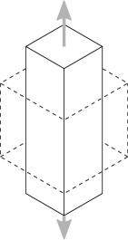
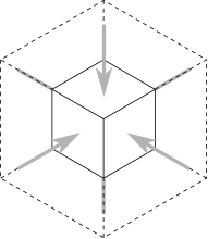
Figure 3: Illustration of the verification tests by uniaxial stretch (left) and hydrostatic compression (right) of an elastic cube.

In the uniaxial test the boundary condition in the tensile direction is a plane constraint with free slip in plane. The other boundaries are free. In the hydrostatic compression test the boundary conditions are dynamically generated unilateral contact constraints. The boundary force is increased linearly with time, by regulating the position of the boundary geometry, while measuring the stress and strain components of equations (32)-(33). All tests are simulated on a uniformly discretised homogeneous isotropic three dimensional solid with varying parameters as described in table 2.

Parameter	Value
side length	$1$ m
${N}_{\text{p}}$	$\left(6^{3},9^{3},11^{3}\right)$
resolution	$1/{N}_{\text{p}}^{3}$ m
influence radii	$2$ $\times$ resolution
mass density	$2000$ kg/m3
Young’s modulus $E$	$\left(10^{6},10^{8}\right)$ Pa
Poisson ratio $\nu$	$\left(0.1,0.25,0.49\right)$
Timestep $h$	$10^{-3}$ s

Table 2: Elastic verification parameters

The simulation result is compared with elasticity theory that for St. Venant-Kirchoff materials imply the following exact relations between applied load and uniform deformation

$${p}_{\text{u}} =\frac{1}{2}{c}_{\text{u}}{\underline{\lambda}}_{\text{u}}\left({\underline{\lambda}}_{\text{u}}^{2}-1\right)$$ (32)

$${p}_{\text{c}} =\frac{1}{2}{c}_{\text{c}}{\underline{\lambda}}_{\text{c}}\left({\underline{\lambda}}_{\text{c}}^{2}-1\right)$$ (33)

where $p=F/A_{0}$ is the load pressure on the boundary, ${c}_{\text{u}}=E$ ${c}_{\text{c}}=\frac{E}{(1-2\nu)}$ are the Young’s and bulk modulus, and ${\underline{\lambda}}_{\text{u}}$ and ${\underline{\lambda}}_{\text{c}}$ are the stretch ratios $l/l_{0}$ of the test-cube with the deformed side-length $l$, initial rest length $l_{0}$ and cross-sectional area $A_{0}$. The simulation results for $E=10^{6}$ Pa and $\nu=0.25$ are presented in figure 4.

For large deformations ($15$ %) the simulated result agrees with the exact solution to an accuracy of $5$ % for uniaxial stretch and $10$ % for hydrostatic compression. The error decrease with size of the deformation and with finer resolution. Observe that for infinitesimal deformations $\frac{1}{2}\underline{\lambda}\left(\underline{\lambda}^{2}-1\right)\approx\Delta l/l_{0}$, Eq.  (32)-(33) approximates to the well-known expressions from Hooke’s law. Increasing the stiffness or resolution further require smaller time-step for numerical stability.

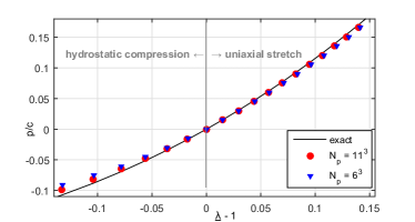
Figure 4: Verification test of elastic response to hydrostatic compression ($\underline{\lambda}<1$) and uniaxial stretch ($\underline{\lambda}>1$) with $E=10^{6}$ Pa, $\nu=0.25$ and ${N}_{\text{p}}=11^{3}$ (circles) and ${N}_{\text{p}}=6^{3}$ (triangles). The analytical solution is represented with a solid curve.

In order to understand the nature of the error the strain field under hydrostatic compression is analysed, see figure 5. The strain field is not uniform through the material as expected but deviate as much as $30$ % and most near the boundary. Enforcing a uniform deformation, by initial particle displacements, produce a perfectly uniform strain and stress field. We thus conclude that the effect is caused by the way that boundary conditions are enforced. See, section 5 for a further discussion on this.

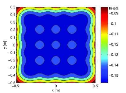
Figure 5: The variation of $\operatorname{tr}(\epsilon)$ through the cross-section of the elastic test cube under hydrostatic compression to $\underline{\lambda}=0.86$.

The errors in the strain distribution propagate to the stress and ultimately to the plastic behaviour also. In particular the deviation from nonuniform strain will lead to a non-vanishing stress deviator in deformations where it is expected to be zero. The mean strain deviatior and its standard deviation in the case of hydrostatic compression is displayed in figure 6.

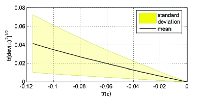
Figure 6: The variation of $\operatorname{tr}[\text{dev}(\epsilon)^{2}]^{1/2}$ during hydrostatic compression.

4.3.2 Plasticity

The Drucker-Prager cap model is tested under hydrostatic and triaxial loading and unloading, following the tests made in [12] with $E=9.0865\cdot 10^{7}$ Pa,$\nu=0.2981$, $c=14$ kPa, $\phi=22^{\circ}$, $W=0.1$, $D=1$ mm²/N. The first test examines the relation between stress and strain while undergoing plastic deformation on the compression cap, see figure 7.

The test produce a permanent deformation of the cube by $\operatorname{tr}{\epsilon}=0.095$ compared to $\operatorname{tr}{\epsilon}=0.12$ in [12]. As can be expected this deviation is due to the deviation of uniform strain, observed in section 4.3.1, that lead to non-vanishing deviatoric stress. Investigating the evolution of the stress invariants, $I_{1}$ and $J_{2}$, in the yield space, it is clear that the compression cap is not reached precisely on the hydrostatic axis and thus yield for a smaller of $I_{1}$. The plastic shear is also not uniform which affect the permanent deformation.

In the triaxial test, a hydrostatic pressure of $100$ kPa is first established. The load along one axis is then increased up to a level where the material yields and while pressure is kept fix. The material is finally unloaded. The simulated evolution of the deviatoric stress as function of strain is displayed in figure 8 for a Drucker-Prager material and in figure 9 for a capped Drucker-Prager material. The simulated Drucker-Prager material is found to yield at a critical stress of $260$ kPa. This is in precise agreement with the analytical prediction from equation (18) with hydrostatic pressure of $100$ kPa. For the capped Drucker-Prager the yield plateau is lower and less pronounced. The difference is expected since the stress reach the compression cap surface before the Drucker-Prager surface. The result show a weak dependency on resolution ${N}_{\text{p}}=2^{3},6^{3}$ and $8^{3}$. The triaxial test can be used to determine the value of the plastic hardening parameter $D$, whereas the maximum compaction parameter, $W$, can be determined from the hydrostatic compression test.

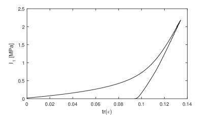
(a) Stress evolution.

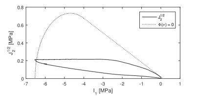
(b) Mean stress evolution and yield surface.

Figure 7: Hydrostatic compression and unloading of an elastoplastic solid cube.

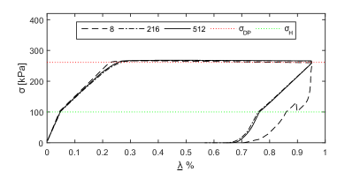
(a) Applied stress over deformation.

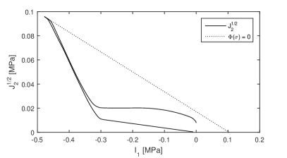
(b) Mean stress evolution and yield surface.

Figure 8: Plastic Drucker-Prager triaxial load and unload.

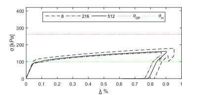
(a) Applied stress over deformation.

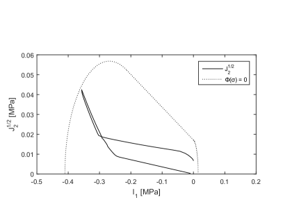
(b) Mean stress evolution and yield surface.

Figure 9: Plastic Cap/Drucker-Prager triaxial load and unload.

4.3.3 Dynamic contacts

Dynamic contact handling is demonstrated by dropping a beam to rest on two thin cylinders and then let if deformed by pressing a larger cylinder down on the beam. The result for an elastic and elastoplastic beam are displayed in Figure 10.

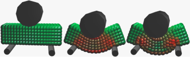
Figure 10: Deformation of an elastic and elastoplastic beam (middle and right from initial state to the left). The color codes the frobenius norm of the strain tensor, ranging from $0$ (green) to $0.20$ (red).

4.4 Multidomain demonstration

In order to demonstrate multidomain capability with the method, two example systems are simulated. The first system is an articulated terrain vehicle with tracked bogies driving over a deformable terrain. Images from simulation of a bogie and of a full vehicle are shown in figure 11. Videos from simulations are available as supplementary material at http://umit.cs.umu.se/elastoplastic/. The vehicle weighs 4 ton and consist of roughly 200 rigid bodies including a front and rear chassis, bogie frames, wheels and track elements. These are interconnected with kinematic constraints to model chassis articulation, bogie and wheel axes, and tracks covering the wheeled bogies. The vehicle drivetrain consist of a engine, torque converter, drive shafts and differentials that distributes the engine power to front and rear part and further between left and right bogies to the wheels. The terrain is modeled as a static trimesh and a rectangular ditch with elastoplastic material. The elastoplastic material parameters are set to $Y=1$ MPa, $v=0.25$, $\phi=22^{\circ}$, $c=1$ kPa, $R_{C}=4$, $T=5$ kPa, $\kappa_{0}=-0.5$ MPa, $D=10^{-6}$, $W=0.2$, $\rho=2000$ kg/m³, which represents a weak and soft forest terrain. The tracked bogie and vehicle create a rutting with permanent deformation and the rut depth can be measured. In the full vehicle simulation the solid is discretised into ${N}_{\text{p}}=2100$ pseudo-particles. The coupled system of vehicle and terrain thus have roughly 7000 degrees of freedom and roughly the same number of constraint equations. With $1$ ms timestep the simulation was of the order $1000$ slower than realtime on a conventional desktop computer and using a single core. It should be emphasised that this measure is based on prototype code with little effort on optimizing it. Also the use of a direct solver for the terrain can be questioned. Both the model uncertainty and spatial discretisation error are many orders in magnitude beyond the accuracy delivered by the solver.

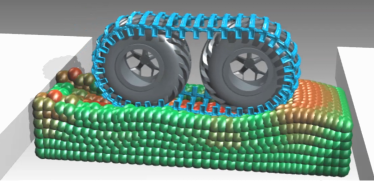
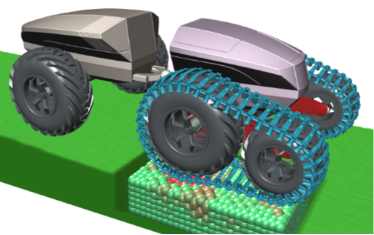
Figure 11: Images from simulation of a tracked bogie (top) and a full terrain vehicle (bottom) passing over a zone with elastoplastic material.

The second demonstration example is a dynamic cone penetration test where a cylindrical weight is dropped repeatedly on a cone measuring its penetration depth. This is one common way of measuring the mechanical properties of terrain. The penetration depth of the cone in simulated for two different cases. The first case is a homogeneous material and the second is material with an embedded rock, represented by a rigid body, as illustrated by figure 12. The colours indicated the magnitude of displacement. The simulated cone penetration is presented in figure 13. The resistance is higher in the ground with an embedded rock, also before the cone actually come in contact with the rock.

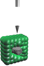
(a) $0s$

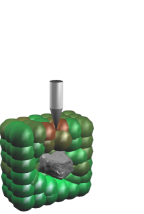
(b) $2.4s$

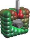
(c) $4.7s$

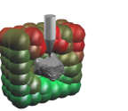
(d) $7.0s$

Figure 12: Image sequence from a simulated cone penetration test on an elastoplastic terrain with an embedded rock.

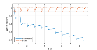
(a) Homogeneous terrain.

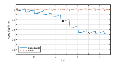
(b) Terrain with embedded rock. The $\times$ indicate the time instances in Figure 12 b-d.

Figure 13: Simulation measurement of a cone penetrometer on elastic and elastoplastic terrain with and without embedded rock.

5 Conclusions

A meshfree elastoplastic solid model is made compatible with nonsmooth multidomain dynamics. The solid appear as a system of constrained particles in a multibody system on the same footing as articulated rigid multibodies and power transmission systems. The particles carry field variables, e.g., the stress and strain tensor, approximated using the moving least squares method. This method provides a continuous field description throughout the solid. The dynamic interaction between the deformable solid, rigid multibodies and other geometric boundaries is modeled by unilateral contact constraints with dry friction. The full system can thus be processed using the same numerical integrator and solver framework without introducing additional coupling equations with unknown parameters and impulsive behaviour can automatically be transmitted instantly through the full and strongly coupled system. This enables fast and stable simulations of complex mechatronic systems with, or interacting with, elastoplastic materials. Demonstration is made with a tracked terrain vehicle driving over deformable terrain using the capped Drucker-Prager model and a cone penetrometer test on terrain with and without embedded rock.

The Jacobian of the deformation constraint is derived and the explicit form is given in Eq. (26). It can be factored to a constant term that can be pre-computed and multiplied with current particle displacements. The computational bottleneck of the simulation lies in solving the block sparse mixed linear complementarity problem (10). With dedicated hardware, parallel factorisation algorithms or using iterative solver for a more approximate solution of the terrain dynamics the performance is expected to be increased by several order in magnitude. Exploring this is left for future work.

The results of numerical experiments of uniform elastic deformations, presented in figure 4 and 5, reveal that the solution deviate from what is expected from analytical solutions. For example, the confining pressure in hydrostatic compression of a cube discretised by $6\times 6\times 6$ particles is underestimated by roughly $10$ % when compressed up to $\Delta V/V=15$ %. The error decrease with reduced time-step and finer spatial discretisation.

The errors are presumably due to the application of mls to the solid dynamics equations on strong form. When the problem involve traction boundary conditions, meshfree collocation methods suffer from poor accuracy and instability [13]. The errors are not located solely to the boundaries but influence also the deformations further in the material, as seen in Figure 5, and cause the second principal deviatoric stress invariant to deviate from zero in hydrostatic pressure.

This affect the plastic behaviour also. The permanent plastic deformation after loading is found to differ by the order of $10$ % and sometimes the material has residual stress that may cause artefacts although none have been observed. Nevertheless, the developed method is applicable to many type of studies where this level of accuracy is acceptable and cannot be increased further anyway because of difficulties in characterising the mechanical properties of the solid material.

This deficiency can be avoided by either using a mixed strong and weak form formulation [13] or applying correction terms of higher order on the boundary particles [30]. Future work should focus on this issue to improve the accuracy of the model. Another area of improvement is to integrate the plastic yield and flow computations with the mixed complementarity problem for the constraint forces and velocity update. This will enable integration with larger time-step for strongly coupled problems than the current predictor-corrector method allow.

Appendix

A. Capped Drucker-Prager yield surface

This supplements Section 3 with further details of the Capped Drucker-Prager yield surfaces in Eq. (18)-(17) illustrated in Figure 2. We follow the smooth cap model of Dolarevic and Ibrahimbegovic [12] with some corrections to the compression cap. The three yield functions are

$$\Phi_{\textsc{\tiny DP}}\left(I_{1},J_{2}\right) =\sqrt{J_{2}}+\frac{\eta}{3}I_{1}-\xi c$$ (34)

$$\Phi_{\textsc{\tiny T}}\left(I_{1},J_{2}\right) =\left(I_{1}-T+R_{\textsc{\tiny T}}\right)^{2}+J_{2}-R^{2}_{\textsc{\tiny T}}$$ (35)

$$\Phi_{\textsc{\tiny C}}\left(I_{1},J_{2},\kappa\right) =\frac{\left[I_{1}-a\left(\kappa\right)\right]^{2}}{R_{\textsc{\tiny C}}^{2}}+J_{2}-b\left(\kappa\right)^{2}$$ (36)

The center, radius and intersection point of the tension cap are

$$C =\frac{T-\frac{3\xi c}{\eta}\sin\left(\varphi\right)}{1-\sin\left(\varphi\right)}$$ (37)

$$R_{t} =T-C$$ (38)

$$I_{t} =\frac{3\xi c}{\eta}-\beta\cos\left(\varphi\right)$$ (39)

where the Drucker-Prager cone angle $\phi=\arctan(\eta)$ in the pressure-shear plane, $T$ is the tension cap cutoff and $\beta=[\left(3\xi c/\eta-C\right)^{2}-R_{t}^{2}]^{1/2}$. The compression cap intersection point is

$$I_{c} =\frac{3\xi c}{\eta}-\frac{3b\left(\kappa\right)}{\eta\sqrt{1.0+\left(\frac{\eta}{3}\right)^{2}R_{c}^{2}}}$$ (40)

and $a\left(\kappa\right)$ and $b\left(\kappa\right)$ are the center and main radius of the compression cap ellipse [12]. The stress gradient of the yield functions are

$$\frac{\partial\Phi_{\textsc{\tiny DP}}}{\partial\bm{\sigma}} =\frac{\bm{s}}{2\sqrt{J_{2}\left(\bm{\sigma}\right)}}+\frac{\eta\left(\phi\right)}{3}\bm{1}$$ (41)

$$\frac{\partial\Phi_{\textsc{\tiny T}}}{\partial\bm{\sigma}} =\bm{s}+2\left(I_{1}-T+R_{t}\right)\bm{1}$$ (42)

$$\frac{\partial\Phi_{\textsc{\tiny C}}}{\partial\bm{\sigma}} =\bm{s}+\frac{2\left(I_{1}-a\left(\kappa\right)\right)}{R^{2}}\bm{1}$$ (43)

References

- [1] Kübler K, Schiehlen W. Two methods of simulator coupling. Mathematical and Computer Modelling of Dynamical Systems, 6(2):93–113, 2000.
- [2] Burgermeister B., Arnold M., Eichberger A. Smooth velocity approximation for constrained systems in real-time simulation Multibody System Dynamics, Vol 26 (1), 1–14, 2011.
- [3] Acary V., Brogliato B. Numerical Methods for Nonsmooth Dynamical Systems: Applications in Mechanics and Electronics. Springer Verlag, 2008.
- [4] Lacoursière C. Ghosts and Machines: Regularized Variational Methods for Interactive Simulations of Multibodies with Dry Frictional Contacts. PhD thesis, Umeå university, 2007.
- [5] Lacoursière C. Regularized, stabilized, variational methods for multibodies. In Dag Fritzson Peter Bunus and Claus Führer, editors, The 48th Scandinavian Conference on Simulation and Modeling (SIMS 2007), 30-31 October, 2007, Göteborg (Särö), Sweden, Linköping Electronic Conference Proceedings, pages 40–48. Linköping University Electronic Press, December 2007.
- [6] Taheri S, Sandu C., Taheri S., Pinto E., Gorsich D. A technical survey on Terramechanics models for tire–terrain interaction used in modeling and simulation of wheeled vehicles Journal of Terramechanics 57, 1–-22, 2015.
- [7] Azimi A., Holz D., Kövecses J., Angeles J., Teichmann M. A Multibody Dynamics Framework for Simulation of Rovers on Soft Terrain J. Comput. Nonlinear Dynam 10(3) , 2015
- [8] Madsen J., Seidl A., Negrut D., Compaction-Based Deformable Terrain Model as an Interface for Real-Time Vehicle Dynamics Simulations SAE World Congress, Detroit, 2013.
- [9] Shoop S. A. Finite element modeling of tire-terrain interaction CRREL Technical Report, ERDC/CRREL TR-01-16, US Army Cold Regions Research and Engineering Laboratory, Hanover, NH, 2001.
- [10] Xia K.. Finite element modeling of tire/terrain interaction: Application to predicting soil compaction and tire mobility Journal of Terramechanics 48, 113–-123, 2013.
- [11] de Souza Neto E. A., Peric D., Owen D. R. J. Computational Methods for Plasticity: Theory and Applications Wiley, Chichester (2008)
- [12] Dolarevic S., Ibrahimbegovic A. A modified three-surface elasto-plastic cap model and its numerical implementation. Comput. Struct., 85(7-8):419–430, April 2007.
- [13] Liu G. R., Gu Y. T. An Introduction to Meshfree Methods and Their Programming Springer Publishing Company, Dordrecht, 2010.
- [14] Nguyena V. P., Rabczukb T., Bordasc S., Duflot M. Meshless methods: A review and computer implementation aspects Mathematics and Computers in Simulation 79, 763–-813, 2008.
- [15] Ullah Z., Augarde C. E. Finite deformation elasto-plastic modelling using an adaptive meshless method. Computers and Structures 118, 39–-52, 2013.
- [16] Belytschko T., Lu Y. Y., Gu L. Element-free galerkin methods. International Journal for Numerical Methods in Engineering, 37(2):229–256, 1994.
- [17] Bornemann F.,Schütte C. Homogenization of Hamiltonian systems with a strong constraining potential. Phys. D, 102(1-2):57–77, 1997.
- [18] Marsden J. E., West M. Discrete mechanics and variational integrators. Acta Numer., 10:357–514, 2001.
- [19] Servin M., Lacoursière C. Rigid body cable for virtual environments. IEEE Transactions on Visualization, 14(4):783–796, 2008.
- [20] Servin M., Lacoursière C., Nordfelth F., Bodin K. Hybrid, multiresolution wires with massless frictional contacts. Visualization and Computer Graphics, IEEE Transactions on, 17(7):970–982.
- [21] Bodin K., Lacoursiere C., Servin M. Constraint fluids. IEEE Transactions on Visualization and Computer Graphics, 18(3):516–526, 2012.
- [22] M. Servin, D. Wang, C. Lacoursière, K. Bodin Examining the smooth and nonsmooth discrete element approach to granular matter Int. J. Numer. Meth. Engng. 97 (2014) 878–902.
- [23] Pang J. S., Stewart D. Differential variational inequalities. Math. Program., 113(2):345–424, 2008.
- [24] Wasfy M., Noor A. Computational strategies for flexible multibody systems. Applied Mechanics Reviews, 56(6):553–613, 2003.
- [25] Algoryx Simulations. AGX Dynamics. September 2015.
- [26] Cottle R., Pang J-S., Stone R. The Linear Complementarity Problem. Computer Science and Scientific Computing. 1992.
- [27] Lacoursière C., Linde M. Spook: a variational time-stepping scheme for rigid multibody systems subject to dry frictional contacts. UMINF report 11.09, Umeå University, 2011.
- [28] Lacoursière C., Linde M. Unpublished work, 2015.
- [29] Neto S, Owen D R J, Perić D. Computational Methods for Plasticity: Theory and Applications. Wiley, Chichester, 2008.
- [30] Miguel J., Onate P. A finite point method for elasticity problems, computers and structures. Computers and Structures, 79:2151–2163, 2001.