On the oscillation-driven cosmological expansion at the post-inflation stage

Abstract

Dynamics of the inflaton scalar field oscillating around a minimum of the singular potentials in the expanding Universe is investigated. Asymptotic formulas are obtained describing the cosmological expansion at the late times. The problem of stability of the oscillations considered and the related phenomenon of the field fragmentation are briefly discussed.

I Introduction

According to the standard inflationary scenario the accelerated expansion of the Universe occurs when the inflaton scalar field $\phi$ is in the slow-roll regime on a sufficiently flat part of the potential $V(\phi)$ Star1 ; Linde1 ; Albrecht ; Linde2 . Such potentials can arise when taking into account quantum corrections in the right-hand side of the Einstein equations Star1 . As the minimum of the potential is approached, the speed of the rolling-down increases, and the scalar field eventually enters the stage of rapid oscillations Kofman . For the potentials having a power-law behavior at the minimum these oscillations have been considered by Turner Tur , who has derived the effective equation of state for them. Later on, Damour and Mukhanov Dam have pointed out that inflation will continue for a time at the oscillation stage too if the potential is non-convex in regions not too far from the minimum. They also have found a nice geometric interpretation of this fact and estimated the amount of inflation occurring at the oscillation stage. This estimation was being improved successively by Liddle and Mazumdar Liddle and Sami Sami .

At the present paper the primary emphasis is on the potentials admitting oscillation-driven inflation, but having singularities at their minima. Singular potentials are intensively discussed in the modern cosmology in the context of the so-called sudden singularities occurring in high derivatives of the metric when the scalar field $\phi$ passes through the minimum of $V(\phi)$ (see, e.g., Barrow1 and references therein). In contrast, we consider the effect of singularities of the inflaton potentials on the cosmological expansion dynamics averaged over the oscillation time scale. The paper is organized as follows. In Section 2, based on the method of averaging, we give a rigorous treatment of the scalar field oscillations in the Friedmann-Robertson-Walker Universe. Using these results, in Section 3 we perform the comparison analysis of the cosmological expansion dynamics at the post-inflation stage for three generic potentials, two of them being singular. In Section 4 some remarks are made concerning stability of the oscillations considered.

II Scalar field oscillations in the expanding Universe

The homogeneous inflaton scalar field $\phi$ in the flat Friedmann-Robertson-Walker Universe is described by the equation

$$\phi_{tt}+3H\phi_{t}+V^{\prime}(\phi)=0,$$ (1)

where $H=a_{t}/a$ is the Hubble parameter, $a(t)$ is the scale factor. If one assumes the Universe is filled with a scalar field $\phi$ only, the evolution of the scale factor $a(t)$ will be governed by the Friedmann equations

$$a_{tt}/a=-\left(4\pi G/3\right)\left(\rho+3p\right),$$ (2)

$$\left(a_{t}/a\right)^{2}=\left(8\pi G/3\right)\rho$$ (3)

with the effective pressure and energy density

$$p=\phi_{t}^{2}/2-V(\phi),\text{\quad}\rho=\phi_{t}^{2}/2+V(\phi).$$ (4)

From Eqs. (2) and (3) it follows that

$$\rho_{t}=-3(a_{t}/a)(p+\rho).$$ (5)

Once the slow-roll stage ends, the inflaton field $\phi(t)$ begins to execute fast damped oscillations around the minimum of the potential $V(\phi)$. Equation (1) describing these oscillations can be treated, in view of Eqs. (3) and (4), as a dissipative dynamical system written in terms of the independent variables $\phi$ and $\phi_{t}$. Let us go from these variables to the other ones, $\theta$ and $\rho$, following the technique of separation of fast and slow motions (see, e.g., Mois ). We set

$$\phi = \varphi(\theta,\rho),$$ (6)

$$\phi_{t} = \omega(\rho)\,\varphi_{\theta}(\theta,\rho),$$ (7)

where $\varphi(\theta,\rho)$ is a $2\pi$-periodic solution of the equation

$$\omega^{2}(\rho)\,\varphi_{\theta\theta}+V^{\prime}(\varphi)=0.$$ (8)

From Eqs. (4), (6), and (7) it follows that the first integral of this equation is just the energy density $\rho$,

$$\frac{1}{2}\,\omega^{2}(\rho)\,\varphi_{\theta}^{2}+V(\varphi)=\rho,$$ (9)

so that

$$\omega^{-1}(\rho)=\frac{1}{\pi\sqrt{2}}\int_{\varphi_{\min}(\rho)}^{\varphi_{\max}(\rho)}\frac{d\varphi}{\sqrt{\rho-V(\varphi)}},$$ (10)

where $V(\varphi_{\min,\text{ }\max})=\rho$. Equations (6)-(10) fully determine the transformation $\left(\phi,\phi_{t}\right)\rightarrow\left(\theta,\rho\right)$.

In order for the above procedure to be self-consistent, Eqs. (6) and (7) must be supplemented by the compatibility condition

$$\varphi_{\theta}\theta_{t}+\varphi_{\rho}\rho_{t}=\omega\varphi_{\theta}.$$ (11)

Equations determining evolution of the variables $\rho$, $\theta$ are derived from Eqs. (5) and (11) with the use of Eqs. (3), (4), and (7):

$$\rho_{t} = -2\sqrt{6\pi G}\rho^{1/2}\omega^{2}(\rho)\varphi_{\theta}^{2},$$ (12)

$$\theta_{t} = \omega(\rho)+2\sqrt{6\pi G}\rho^{1/2}\omega^{2}(\rho)\varphi_{\rho}\varphi_{\theta}.$$ (13)

It should be pointed out that these equations are exact and fully equivalent to Eq. (1). The similar, but more cumbersome equations can be obtained for the polar coordinates of the variables $\phi$, $\phi_{t}$ Ren .

Integrating $p+\rho=\omega^{2}(\rho)\varphi_{\theta}^{2}$ over $\theta$ from $0$ to $2\pi$ and denoting $\bar{p}=\left(2\pi\right)^{-1}\int_{0}^{2\pi}p(\theta,\rho)\,d\theta$ we immediately obtain the Turner’s formula for the adiabatic index:

$$\gamma(\rho)=1+\frac{\bar{p}(\rho)}{\rho}=\frac{\sqrt{2}\omega(\rho)}{\pi\rho}\int_{\varphi_{\min}(\rho)}^{\varphi_{\max}(\rho)}\sqrt{\rho-V(\varphi)}\,d\varphi.$$ (14)

This formula can be also derived with the help of the action-angle variables Masso . As seen from Eq. (2), the adiabatic index determines dynamics of the cosmological expansion: the Universe will expand with acceleration if $\gamma<2/3$, and with deceleration if $\gamma>2/3$.

The system of equations (12), (13) belongs to the class of systems with a rotating phase. If the field oscillations are sufficiently fast in comparison with the rate of the cosmological expansion, i.e., $H/\omega\sim\varepsilon\ll 1$, the generalized averaging method will be applicable for simplification of the system. In general, the method consists in going from $\theta,\rho$ to the new, ”averaged”, variables $\bar{\theta},\bar{\rho}$ with the help of asymptotic power series in $\varepsilon$ Mois ; Nayf . In the lowest order we have $\rho=\bar{\rho}+O(\varepsilon),\;\theta=\bar{\theta}+O(\varepsilon)$, and evolution equations for $\bar{\rho}$ and $\bar{\theta}$ are derived for once by averaging over the period $2\pi$ of the right-hand sides of Eqs. (12) and (13), which corresponds to the Van der Pol approximation. As a result we find

$$\rho_{t} = -2\sqrt{6\pi G}\,\rho^{3/2}\gamma(\rho),$$ (15)

$$\theta_{t} = \omega(\rho),$$ (16)

where we have dropped the bar signs and neglected of the term arising from averaging of the second term in Eq. (13). The latter is caused by the neglect of the next order term ($\sim\varepsilon^{2}$) in Eq. (15) resulting in the error in $\rho$ of the order of $\varepsilon^{2}t$. This situation is typical when considering the systems with a rotating phase in the lowest order approximation (see, e.g., Mois ). Our following analysis is based on system (15), (16).

III The potentials

Here we will deal with three generic potentials having very similar shapes (sketched in Fig. 1), but essentially different behavior at the minima. Namely, we examine the canonical $\phi^{2}-\phi^{4}$ potential,

$$V(\phi)=\frac{m^{2}}{2}\phi^{2}-\frac{\lambda}{4}\phi^{4},$$ (17)

the logarithmic potential,

$$V(\phi)=\frac{m^{2}}{2}\phi^{2}\left(1-\ln\frac{\phi^{2}}{\sigma^{2}}\right),$$ (18)

and the fractional-power potential,

$$V(\phi)=-\frac{m^{2}}{2}\phi^{2}+\frac{3\lambda}{4}\phi^{4/3}.$$ (19)

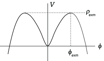
Figure 1: Sketch of the shape of potentials (17)-(19).

While the first potential is evidently regular, the two potentials last named have singularities at the minimum, $\left|V^{\prime\prime}(\phi)\right|\rightarrow\infty\;(\phi\rightarrow 0)$. The logarithmic potentials currently appear in inflationary cosmology Barrow2 and in some supersymmetric extensions of the Standard model (e.g., flat direction potentials in the gravity mediated supersymmetric breaking scenario Enq ). The logarithmic terms arise due to quantum corrections to the bare inflaton mass. The fractional-power potentials are also considered in cosmology Barrow1 ; Hari .

Let us investigate the dynamics of cosmological expansion at the stage of scalar field oscillations for each of the above potentials.

III.1 The $\mathbf{\phi^{2}-\phi^{4}}$ potential

For this potential all quantities can be evaluated exactly. From Eqs. (10) and (14) we find

$$\frac{\omega}{m}=\frac{\pi}{2K(\varkappa)\sqrt{1+\varkappa^{2}}},$$ (20)

$$\gamma=\frac{2}{3\varkappa^{2}K(\varkappa)}\left[\left(1+\varkappa^{2}\right)E(\varkappa)-\left(1-\varkappa^{2}\right)K(\varkappa)\right],$$ (21)

where $K(\varkappa)$ and $E(\varkappa)$ are complete elliptic integrals,

$$\varkappa=\frac{1}{\sqrt{\rho/\rho_{\rm{exm}}}}\left(1-\sqrt{1-\rho/\rho_{\rm{exm}}}\right),$$ (22)

$\rho_{\rm{exm}}=V(\phi_{\rm{exm}})=m^{4}/\left(4\lambda\right),\;\phi_{\rm{exm}}\equiv\varphi_{\rm{exm}}=m/\sqrt{\lambda}$. Since $0<\rho/\rho_{\rm{exm}}<1$, one has $0<\varkappa<1$. Figure 2 illustrates the corresponding curves. It is seen that $\gamma=2/3$ is achieved at the transition point $\rho_{\rm{tr}}/\rho_{\rm{exm}}\approx 0.914$.

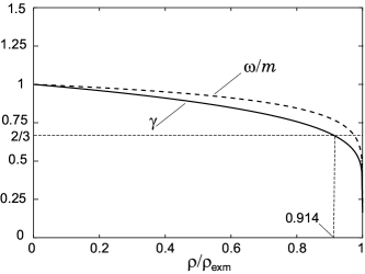
Figure 2: The oscillation frequency and adiabatic index for potential (17).

The damped field oscillations are given by

$$\phi(t)=\varphi(\theta,\rho)=\varphi_{\max}(\rho)\,{\rm sn}\left(\frac{2K(\varkappa)}{\pi}\theta,\varkappa\right),$$ (23)

where

$$\varphi_{\max}=\varphi_{\rm{exm}}\sqrt{\frac{2\varkappa^{2}}{1+\varkappa^{2}}}.$$ (24)

At the late times $\tau=\sqrt{6\pi G\rho_{\rm{exm}}}\;t\gg 1$ the energy density is small, $\varrho=\rho/\rho_{\rm{exm}}\ll 1$, so that

$$\frac{\omega}{m}\approx 1-\frac{3}{16}\varrho,\qquad\gamma\approx 1-\frac{3}{32}\varrho,$$ (25)

$$\frac{\varphi_{\max}}{\varphi_{\rm{exm}}}\approx\frac{\sqrt{2}}{2}\varrho^{1/2},\qquad\bar{p}\approx-\frac{3m^{4}}{128\lambda}\varrho^{2}.$$ (26)

In this case the general integral of Eq. (15) has the form

$$\varrho^{-1/2}+\frac{\sqrt{6}}{16}\ln\frac{1-\frac{\sqrt{6}}{8}\varrho^{1/2}}{1+\frac{\sqrt{6}}{8}\varrho^{1/2}}+const=\tau.$$ (27)

The constant in (27) is determined by the initial conditions. It is seen that their effect is much more essential at the late times than the impact of the logarithmic term that tends to zero as $\varrho\rightarrow 0$. Ignoring the initial conditions and, hence, the logarithmic term, we obtain asymptotically

$$\varrho\sim\tau^{-2},\quad a\propto\varrho^{-1/3}\propto\tau^{2/3}.$$ (28)

Thus, the scalar field, oscillating around a quadratic-power minimum of the regular potential, behaves as a non-relativistic matter Star2 .

III.2 The logarithmic potential

Consider now potential (18) having weak logarithmic singularity at the origin. In this case $\rho_{\rm{exm}}=m^{2}\sigma^{2}/2$, $\varphi_{\rm{exm}}=\sigma$, $\rho_{\rm{tr}}/\rho_{\rm{exm}}\approx 0.854$ (see Fig. 3). For the late times, $\tau\gg 1$, $\varrho=\rho/\rho_{\rm{exm}}\ll 1$, from (10), (14) we obtain the asymptotic expansions

$$\omega/m=\Delta\left(1-a_{2}\Delta^{-2}-a_{4}\Delta^{-4}+O(\Delta^{-6})\right),$$ (29)

$$\gamma=1-b_{2}\Delta^{-2}-b_{4}\Delta^{-4}+O(\Delta^{-6}),$$ (30)

where $\Delta^{2}=1-\ln\left(\varphi_{\max}/\varphi_{\rm{exm}}\right)^{2}\gg 1,$ $\Delta^{2}e^{1-\Delta^{2}}=\varrho\ll 1$.

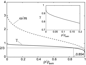
Figure 3: The oscillation frequency and adiabatic index for potential (18).

Calculation gives: $a_{2}=1-\ln 2\approx 0.307,$ $a_{4}=\pi^{2}/8-\ln 4+(1/2)\ln^{2}2\approx 0.088,$ $b_{2}=1/2,$ $b_{4}=3/4-\ln 2\approx 0.057$. Restricting ourselves to the leading terms of these expansions we find

$$\frac{\omega}{m}\approx\sqrt{-\ln\varrho},\qquad\gamma\approx 1+\frac{1}{2\ln\varrho},$$ (31)

$$\frac{\varphi_{\max}}{\varphi_{\rm{exm}}}\approx\sqrt{-\frac{\varrho}{\ln\varrho}},\qquad\bar{p}\approx\frac{m^{2}\sigma^{2}}{4}\frac{\varrho}{\ln\varrho}.$$ (32)

In this approximation the general integral of Eq. (15) is given by

$$\varrho^{-1/2}\left(1-\frac{1}{2\ln\varrho}+O\left(\ln^{-2}\varrho\right)\right)+const=\tau$$ (33)

Ignoring the effect of initial conditions we obtain asymptotically

$$\varrho\sim\tau^{-2}\left(1+1/\ln\tau^{2}\right),\quad a\propto\tau^{2/3}\left(\ln\tau\right)^{1/6}.$$ (34)

Surprisingly, the field oscillations are still sinusoidal,

$$\phi(t)=\varphi(\theta,\rho)\sim\varphi_{\max}(\rho)\sin\theta,$$ (35)

but with the frequency increasing as $\sqrt{\ln\tau}$. We thus conclude that expansion dynamics with potential (18) is very similar to that with potential (17).

III.3 The fractional-power potential

Let us examine potential (19) having strong fractional-power singularity. In this case $\rho_{\rm{exm}}=\lambda^{3}/\left(4m^{4}\right)$, $\varphi_{\rm{exm}}=\lambda^{3/2}/m^{3}$, $\rho_{\rm{tr}}/\rho_{\rm{exm}}\approx 0.578$ (see Fig. 4).

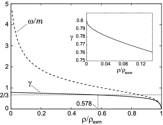
Figure 4: The oscillation frequency and adiabatic index for potential (19).

The corresponding asymptotic expansions for the late times are given by

$$\omega/m=c_{0}\delta^{-1/3}\left(1-c_{2}\delta^{2/3}-c_{4}\delta^{4/3}+O(\delta^{2})\right),$$ (36)

$$\gamma=d_{0}\left(1-d_{2}\delta^{2/3}-d_{4}\delta^{4/3}+O(\delta^{2})\right),$$ (37)

where $\delta=\varphi_{\max}/\varphi_{\rm{exm}}\ll 1,$ $3\delta^{4/3}-2\delta^{2}=\rho/\rho_{\rm{exm}}=\varrho\ll 1,$ $c_{0}\approx 1.071,$ $c_{2}\approx 0.441,$ $c_{4}\approx 0.101,$ $d_{0}=4/5,$ $d_{2}\approx 0.174,$ $d_{4}\approx 0.122$. Notice that the above values of $d_{0}$ and $d_{2}$ can be also derived from formula (16) of Ref. Tur , obtained for the case of a more general potential.

Taking into account in (36)-(37) the leading terms only, we find

$$\frac{\omega}{m}\approx c_{0}\left(\frac{\varrho}{3}\right)^{-1/4},\quad\gamma\approx\frac{4}{5}\left[1-d_{2}\left(\frac{\varrho}{3}\right)^{1/2}\right],$$ (38)

$$\frac{\varphi_{\max}}{\varphi_{\rm{exm}}}\approx\left(\frac{\varrho}{3}\right)^{3/4},\;\bar{p}\approx-\frac{\lambda^{3}}{20m^{4}}\varrho\left[1+4d_{2}\left(\frac{\varrho}{3}\right)^{1/2}\right].$$ (39)

With (38), the general integral of Eq. (15) takes the form

$$\varrho^{-1/2}\left(1-\frac{d_{2}}{\sqrt{3}}\varrho^{1/2}\ln\varrho^{1/2}+O(\varrho)\right)+const=\frac{4}{5}\tau,$$ (40)

so that we obtain asymptotically

$$\varrho\sim\frac{25}{16\tau^{2}}\left(1+\frac{5d_{2}}{2\sqrt{3}}\frac{\ln\tau}{\tau}\right),\quad a\propto\tau^{5/6}.$$ (41)

The field oscillations are essentially non-sinusoidal,

$$\phi(t)=\varphi(\theta,\rho)\sim\varphi_{\max}(\rho)\cos^{3}\psi(\theta,\rho),$$ (42)

where $\psi(\theta,\rho)$ is determined by the elliptic integrals,

$$2E\left(\psi,\sqrt{2}/2\right)-F\left(\psi,\sqrt{2}/2\right)$$ (43)

$$= \left(\sqrt{3}/3\right)\left(\omega/m\right)^{-1}\left(\varphi_{\max}/\varphi_{\rm{exm}}\right)^{-1/3}\theta.$$

It is seen that in this case the scalar field dynamics and the rate of the oscillation-driven cosmological expansion differ drastically from those for potentials (17), (18).

IV Concluding remarks

The above results were obtained under the assumption that the spatially uniform oscillations conserve their coherence over a long period of time. This means these oscillations were assumed to be stable or at least quasistable. To examine the stability one must proceed, instead of (1), from the full Klein-Gordon equation

$$\phi_{tt}+3H\phi_{t}-a^{-2}\Delta\phi+V^{\prime}(\phi)=0.$$ (44)

Consider small perturbations around spatially uniform oscillations,

$$\phi(t,\mathbf{r})=\phi(t)+\delta\phi(t,\mathbf{r}),\qquad\left|\delta\phi\right|\ll\left|\phi\right|.$$ (45)

Setting

$$\phi(t)=\varphi(\theta,\rho),$$ (46)

$$\delta\phi(t,\mathbf{r})=a^{-3/2}(\rho)\,\omega^{-1/2}(\rho)\int Y(\theta,\mathbf{k})e^{i\mathbf{kr}}d\mathbf{k,}$$ (47)

in the linear approximation we arrive at the equation

$$d^{2}Y/d\theta^{2}+\omega^{-2}\left[k_{\rm ph}^{2}+V^{\prime\prime}(\varphi(\theta,\rho))\right]Y=0,$$ (48)

where ${k_{\rm ph}}=k/a$ is the physical wavenumber, and the terms of the second order in $\varepsilon\sim H/\omega$ were neglected. The dependence $a(\rho)$ and slow evolution of $\rho(\theta)$ are determined by the equations

$$a_{\rho}/a=-\left(3\rho\gamma(\rho)\right)^{-1},\quad\rho_{\theta}/\rho=-3\left(H/\omega\right)\gamma(\rho),$$ (49)

resulting from (3), (15), and (16).

Since $\varphi(\theta,\rho)$ is a $2\pi$-periodic function in $\theta$ satisfying Eq. (8), equation (48) belongs to the class of the Hill’s equations with a slowly varying parameter. If $V^{\prime\prime}(\varphi)$ becomes infinite periodically, Eq. (48) will be singular Hill’s equation. For potentials (18), (19) the singular Hill’s equations with constant parameters were investigated in Refs. Kutv1 ; Kutv2 ; Kutv3 where the structure of resonance zones over the $k_{\rm ph}^{2},\varphi_{\max}^{2}$-plane was revealed. It turns out that for the sufficiently large $\left(k_{\rm ph}/m\right)^{2}$ there exists a sequence of the narrow resonance zones with very small values of the Floquet exponent, while in the domain $\left(k_{\rm ph}/m\right)^{2}\sim 1$ one has a wide resonance zone where the exponent is significantly higher. As the Universe expands, $k_{\rm ph}^{2}$ and $\varphi_{\max}^{2}$ decreases. The corresponding points on the $k_{\rm ph}^{2},\varphi_{\max}^{2}$-plane move along the trajectories representing evolution of the perturbation $k$-modes for a given initial $\varphi_{\max}^{2}$. From the start these points cross rapidly the narrow resonance zones not giving $k$-modes the chance to be significantly amplified. With time the speed of the points decreases, and eventually the points enter slowly the domain $\left(k_{\rm ph}/m\right)^{2}\sim 1$ where the $k$-modes begin to grow exponentially. At the nonlinear stage this results in decay of the spatially uniform field $\phi(t)$ into oscillating localized lumps, the pulsons (oscillons). This phenomenon was observed in numerical experiments in Refs. Enq2 ; Amin . Notice that in the case of the logarithmic potential the scale $\left(k_{\rm ph}/m\right)^{2}\sim 1$ corresponds to the size of the gaussian-like pulson being a solution of Eq. (44) with $H=0$. It is clear that sufficiently massive pulsons should be considered as selfgravitating objects, gravipulsons Kutv4 , disturbing significantly the Friedmann-Robertson-Walker metric. Thus the results of the previous sections are valid only up to the beginning of the field fragmentation stage.

References

- (1) A.A. Starobinsky, ”A new type of isotropic cosmological models without singularity”, Phys. Lett. B 91, 99 (1980).
- (2) A.D. Linde, ”A new inflationary universe scenario: A possible solution of the horizon, flatness, homogeneity, isotropy and primordial monopole problems”, Phys. Lett. B 108, 389 (1982).
- (3) A. Albrecht and P. Steinhardt, ”Cosmology for Grand Unified Theories with radiatively induced symmetry breaking”, Phys. Rev. Lett. 48, 1220 (1982).
- (4) A.D. Linde, ”Chaotic inflation”, Phys. Lett. B 129, 177 (1983).
- (5) L. Kofman, A. Linde, and A.A. Starobinsky, ”Reheating after inflation”, Phys. Rev. Lett. 73, 3195 (1994).
- (6) M.S. Turner, ”Coherent scalar-field oscillations in an expanding universe”, Phys. Rev. D 28, 1243 (1983).
- (7) T. Damour and V.F. Mukhanov, ”Inflation without slow roll”, Phys. Rev. Lett. 80, 3440 (1998).
- (8) A.R. Liddle and A. Mazumdar, ”Inflation during oscillations of the inflaton”, Phys. Rev. D 58, 083508 (1998).
- (9) M. Sami, ”Inflation with oscillations”, Gravitation & Cosmology, 8, 309 (2002).
- (10) J.D. Barrow and A.A.H. Graham, ”Singular inflation”, Phys. Rev. D 91, 083513 (2015).
- (11) N.N. Moiseev, Asymptotical Methods of Nonlinear Mechanics (Nauka, Moskva, 1981), in Russian.
- (12) A.D. Rendall, ”Late-time oscillatory behaviour for self-gravitating scalar fields”, Class. Quantum Grav. 24, 667 (2007).
- (13) E. Masso, F. Rota, and G. Zsembinszki, ”Scalar field oscillations contributing to dark energy”, Phys. Rev. D 72, 084007 (2005).
- (14) A.H. Nayfeh, Perturbation Methods (John Wiley & Sons, 1973).
- (15) J.D. Barrow and P. Parsons, ”Inflationary models with logarithmic potentials”, Phys. Rev. D 52, 5576 (1995).
- (16) K. Enqvist and J. McDonald, ”Q-balls and baryogenesis in the MSSM”, Phys. Lett. B 425, 309 (1998).
- (17) K. Harigaya, M. Ibe, K. Schmitz, and T.T. Yanagida, ”Dynamical fractional chaotic inflation”, Phys. Rev. D 90, 123524 (2014).
- (18) A.A. Starobinsky, ”On the nonsingular isotropic cosmological model”, Sov. Astron. Lett. 4, 82 (1978).
- (19) V.A. Koutvitsky and E.M. Maslov, ”Parametric instability of the real scalar pulsons”, Phys. Lett. A 336, 31 (2005).
- (20) V.A. Koutvitsky and E.M. Maslov, ”Instability of coherent states of a real scalar field”, J. Math. Phys. (N.Y.) 47, 022302 (2006).
- (21) V.A. Koutvitsky and E.M. Maslov, ”The singular Hill equation and generalized Lindemann-Stieltjes method”, J. Math. Sci. 208, 222 (2015).
- (22) K. Enqvist, S. Kasuya, and A. Mazumdar, ”Inflatonic solitons in running mass inflaton”, Phys. Rev. D 66, 043505 (2002).
- (23) M.A. Amin, R. Easther, H. Finkel, R. Flauger, and M.P. Hertzberg, ”Oscillons after inflation”, Phys. Rev. Lett. 108, 241302 (2012).
- (24) V.A. Koutvitsky and E.M. Maslov, ”Gravipulsons”, Phys. Rev. D 83, 124028 (2011).