Practical Interpolation for Spectrum Cartography through Local Path Loss Modeling

Abstract

A fundamental building block for supporting better utilization of radio spectrum involves predicting the impact that an emitter will have at different geographic locations. To this end, fixed sensors can be deployed to spatially sample the RF environment over an area of interest, with interpolation methods used to infer received power at locations between sensors. This paper describes a radio map interpolation method that exploits the known properties of most path loss models, with the aim of minimizing the RMS errors in predicted dB-power. We show that the results come very close to those for ideal Simple Kriging. Moreover, the method is simpler in terms of real-time computation by the network and it requires no knowledge of the spatial correlation of shadow fading. Our analysis of the method is general, but we exemplify it for a specific network geometry, comprising a grid-like pattern of sensors. We also provide comparisons to other widely used interpolation methods.

I Introduction

There are several hurdles facing the vision of open and dynamic sharing of spectrum[1]. Perhaps the foremost challenge is the need to create a database of geographical radio maps with information such as location, frequency, and perceived radio power levels[2, 3]. To build such a detailed radio map, radio power from emitters can be measured using a distributed collection of spectrum sensors that span a region of interest. The set of sensor measurements can be processed at a logically central database and interpolated over the large area to build the radio map. The use of radio maps can be extended to applications such as spectrum usage policing, network planning and deployment, and informing spectrum marketplaces.

In this paper, we examine the problem of constructing a radio map that contains estimates of the RF received power in a specified frequency band over a network’s coverage area. As a starting point for our analysis, we assume that there is a single emitter, and all sensors scan the same frequency band, where each of the sensors measures and reports the power received from the emitter. We initially assume, moreover, that the emitter location is known. The position of an emitter can be determined, for example, using any of the numerous emitter localization methods that are common practice [4, 5, 6]. By studying this case in depth, we will uncover results that permit the cases of unknown emitter location and multiple emitters to be treated as well.

We begin the paper in Section II by briefly summarizing the relevant literature. In Section III, we describe the propagation model associated with typical outdoor wireless environments, and show how it suggests a possible approach to optimal interpolation, which we call the Stochastic Method (SM). In Section IV, we derive the root-mean square (RMS) interpolation error for SM under ideal circumstances (we call this case SM-0) and then show it to be equivalent to a basic form of Kriging, which is referred to as Simple Kriging[7]. Since SM-0 requires knowledge that might not be available in practice, we then discuss two approaches for reducing SM to practice: SM-1, which is possible but requires special knowledge of the propagation environment and considerable real-time calculation; and SM-2 which requires neither. In Section V, we quantify the RMS errors for a particular sensor network geometry, showing that SM-1 and SM-2 are very close to each other in performance and only slightly less accurate than the ideal SM-0. We also compare these algorithms with other traditional interpolation methods, and show that SM-2 gives the best tradeoff between accuracy and simplicity. We summarize our findings and their extensions in Section VI, and conclude the paper in Section VII.

II Related Work

Spectrum mapping or spectrum cartography has been applied to different aspects of wireless networks, ranging from estimating radio coverage to wireless network planning[8], mesh/multi-hop networks[9], radio tomographic imaging[10], cognitive radio networks [11, 12, 13], and LTE carrier aggregation[14]. A related application of spectrum mapping involves the need to detect anomalous emitters and to quantify their impact on radio power levels across a geographic area. As such, there are many different areas of related work, including spectrum scanning, signal detection in complex radio environments, and multi-dimensional interpolation. In the area of spectrum scanning, recent work such as [15], explore scheduling a spectrum sensor’s time-frequency scanning across a large swath of bandwidth in hopes of detecting an anomalous signal. The problem of detecting signals in a variety of fading environments (including Rayleigh, Rican and Nakagami channels) was explored in [16]. To combat the uncertainties caused by fading channels in performing signal detection and to support the estimation of a emitter’s impact spatially, it is desirable to use multiple sensors cooperatively. For example, in [17], the authors examine an approach that leverages measurements across an area to decide whether the signal pattern across the region suggests the presence of an anomalous signal, while [18] explores collaborative detection of primary user TV signals in dynamic spectrum access (DSA).

Over the past few decades, radio path loss prediction has been studied using a variety of methods, such as theoretical models, stochastic fading models, interpolation/mapping methods, measurement based/correlated models, and geostatistical models [19]. Basic path loss and stochastic fading models assume prior knowledge and can perform well in specific circumstances. However, they are costly in terms of the time and data acquisition needed to tune them accurately to address other cases [20]. On the other hand, measurement-based models like interpolation and geostatistical methods use measurements from active sensor nodes to estimate physical parameters for given circumstances. In our study, we introduce a practical version of this approach to radio mapping that involves local estimation of path loss parameters to ultimately arrive at better radio map interpolation.

In previous work, global interpolation techniques - Kriging and thin-plate splines - have been studied for spectrum cartography. Under these techniques, measurements from the entire set of sensors are collected and processed at a central location. Kriging is a reliable approach based on the best linear unbiased estimator (BLUE) [7]. Its variants, such as Kriged Kalman filter (universal Kriging) [21], and ordinary Kriging [22, 12] have been widely studied. But these assume first- and second-order stationarity of the spatial data, which is not generally applicable in realistic environments. The use of thin-plate splines, on the other hand, is based on radial basis functions and does not make any channel assumptions. While this approach performs well, even in the absence of precise frequency and bandwidth information, unfortunately the computational complexity increases enormously with the number of sensors and basis functions [22, 23, 24, 13].

In contrast, local spatial interpolation techniques consider only those sensors and their measurements that neighbor the location of interest, and therefore deal well with local changes or variations in the environment, as well as with directional antennas used at emitters. Amongst the local interpolation techniques, Nearest Neighbor (NN), linear interpolation, and Natural Neighbor (NaN) are simple to implement. Unfortunately, while simple to implement, these methods may not be suitable when the characteristics underlying the data changes quickly between nodes or because sensors are often only sparsely positioned[25, 26]. Inverse Distance Weighting (IDW), which is a close relative to the approach we present in this paper, offers a simple and effective form of local spatial interpolation [27, 14], but does not involve local path loss parameter estimation.

III Radio Mapping Approach

The mapping approach described here exploits the mathematical structure of most terrestrial path loss models, which are based on numerous measurement and modeling campaigns over many years. To be specific, the majority of path loss models published for outdoor environments are of the form $PL(d)=B+\Gamma log(d/d_{r})+S$, where $B$ and $\Gamma$ are constants that depend on frequency, antenna heights and gains, and terrain details; $S$ is the statistical variation of path loss about $[B+\Gamma log(d/d_{r})]$ over all Tx-Rx separations of distance $d$. Here, $d_{r}$ is a reference distance, which we will assume, for convenience only, to be 1 m. Path loss models having this form can be found, for example, in [20, 28, 29, 19, 30, 31]. It is customary to regard $[B+\Gamma log(d/d_{r})]$ as the median path loss for distance $d$, and $S$ as shadow fading, typically modeled as a zero-mean Gaussian random process over the environment. Finally, the received power at a given point on the terrain can be written as, $P_{r}=P_{t}+PL(d)$, which is the quantity to be mapped. Here, $P_{r}$ corresponds to receive power, and $P_{t}$ is the transmit power. Invoking the generic path loss form assumed here, $P_{r}$ is

$$P_{r}=A+\Gamma\log(d/d_{r})+S,$$ (1)

where $A=P_{t}+B$.

The constants $A$ and $\Gamma$ are context-specific in that they depend on the transmitted power and the terrain features over the areas to be mapped. In an environment filled with sensors, they can be computed by the network for any small (local) area by measuring received power at $n$ nearby sensors and performing least-squares estimation (LSE) or other forms of estimation[32, 33]. With $A$ and $\Gamma$ thus quantified, the median received power

$$P_{m}=A+\Gamma\log(d/d_{r}).$$ (2)

can then be computed for any given point within the local area, and thus only $S$ needs to be further estimated at that location of interest. This can be achieved by measuring $S$ at each of the $n$ nearby sensors (i.e., by subtracting the median at the sensor from the measured power) and then forming an $n$-fold weighted sum of the resulting $S$-estimates. This is the essence of our approach, which we describe in detail in later sections, and can be applied to any and all points within the coverage area to create the radio map.

For finite $n$, the estimates of $A$ and $\Gamma$ will be imperfect due to the corrupting effects of the random shadow fading, with the estimates tending to improve as $n$ increases. We require that $n>2$ in all cases and later in this paper will examine a specific scenario wherein $n=4$. We will also propose a simple weighting scheme for estimating $S$ at a given point (which yields a powerful variant of inverse distance weighting, IDW) that does not require knowing the spatial statistics of shadow fading; and we will see that, in terms of RF power estimation accuracy, the results are close to a best-case bound, which we will derive.

IV The Stochastic Method

In this section, we present the heart of our approach to performing the underlying interpolations associated with estimating received power. We start by first providing a quick background discussion regarding the spatial characteristics of shadow fading, then move to presenting the idealized form of our interpolation approach, which includes analyzing the first and second moments of shadow fading at an arbitrary point.

IV-A Spatial Correlation of Shadow Fading

The interpolation approach that we will describe will involve: (i) using in-field measurements to estimate the ‘deterministic’ part of $P_{r}$ at a given point; and (ii) focus on estimating the ‘random’ part, $S$, at the point of interest. One can envision the shadow fading component as a two-dimensional stochastic process over the terrain, where $S$ at any point is a Gaussian random variable of zero mean and standard deviation $\sigma$; and the relationship between $S$-values at any two points $i$ and $j$ can be characterized by an autocorrelation function,

$$<S_{i}S_{j}>=c_{ij},$$ (3)

where $<X>$ denotes the expected value of $X$. The optimal way to estimate $S$ at a location between measurement points (sensors) is to know and exploit the correlation properties of $S$ over the terrain, and hence we call this the stochastic method (SM).

A popular formulation for $c_{ij}$ that is simple to use and supported by data in the literature [34], is the decaying exponential,

$$c_{ij}=\sigma^{2}\exp\left(-\frac{d_{ij}}{X_{c}}\right),$$ (4)

where $d_{ij}$ is the physical distance between points $i$ and $j$, and $X_{c}$ is the so-called correlation distance of shadow fading on the terrain. The value of this parameter depends on the type of terrain, and empirical results have been reported for different environments [35, 36, 9].

In our computations of RMS interpolation error, we will invoke the above correlation coefficient as well as others, showing that the precise shape of the function is not a first-order concern in the underlying problem.

IV-B The Ideal Case: SM-0

Assume that $P_{r}$ is to be estimated at a given point on the terrain (labeled as point 0), which is surrounded by $n$ measuring sensors $(n>2)$. The parameters $A$ and $\Gamma$ are estimated from the $n$ measurements of received power, and will be imperfect estimates due to the $S$-values, which act like additive noise. To obtain a theoretical best-case accuracy, however, we assume at first that these estimates are perfect. Therefore, the median value of $P_{r}$ at point 0 is exact, and the network need only predict $S_{0}$ ($S$ at point 0). To quantify the minimal RMS error in this prediction, we use the mathematics of multivariate Gaussian distributions: Assuming that $S_{1},..,S_{n}$ are measured precisely at the sensors, $S_{0}$ is modeled as

$$[S_{0}|S_{1},..,S_{n}]\simeq\mu_{0}+\sigma_{0}u,$$ (5)

where $\mu_{0}$ is the mean of $S_{0}$ conditioned on $S_{1},..,S_{n}$ and is a weighted sum over these $S$-values; $u$ is a zero-mean, unit-variance Gaussian random variate; and $\sigma_{0}$ is the standard deviation of the variation about the mean. We will show that the weights over the $n$ $S$-values can be determined if its correlation is known. Thus, in the ideal case, the expected value of $S_{0}$ can be known, in addition to the median of $P_{r}$. This leaves only $\sigma_{0}u$ as the unknowable component of $P_{r}$. Thus, $\sigma_{0}$ is the irreducible RMS error in interpolating $P_{r}$ from the sensor measurements.

It is worth noting that the above approach is equivalent to a basic form of Kriging, which is often referred to as Simple Kriging[37]. We show in Section -A of the Appendix that the minimum RMS error is equivalent to the RMS error obtained from Simple Kriging, where the bias term is precisely known.

IV-C Determining $\mu_{0}$ and $\sigma_{0}$

For the ideal case, SM-0, the environmental parameters $A$, $\Gamma$, and shadow fading values at $n$ sensors are perfectly known. Thus, $P_{r,0}$ at point 0 is given as

$$P_{r,0}=A+\Gamma\log(d_{0}/d_{r})+[\mu_{0}+\sigma_{0}u],$$ (6)

where $d_{0}$ is the distance from point 0 to the emitter, and the bracketed term corresponds to the shadow fading component, (5).

Under the ideal conditions assumed, we can determine $\mu_{0}$ and $\sigma_{0}$ exactly, since $\mathbf{S}=[S_{1},\cdots,S_{n}]$ is an $n$-fold set of zero-mean Gaussian variates of known correlation matrix. The joint probability density function (pdf) of this set is [38]

$$f_{S}(s)=\left((2\pi)^{n}|\bm{C_{n}}|\right)^{-1/2}\exp\left(-\frac{1}{2}(\bm{S^{T}C_{n}S})\right)$$ (7)

where $\bm{C_{n}}$ is $n\times n$ correlation matrix of $\bm{S}$ with determinant $|\bm{C_{n}}|$ and each of its elements is computed by (3). Thus, from multivariate Gaussian statistics[39], $[S_{0}|\mathbf{S}]$ has mean $\mu_{0}$ and standard deviation $\sigma_{0}$ given by

$$\mu_{0}=(\bm{c_{0}^{T}C_{n}^{-1}})\bm{S},$$ (8)

$$\sigma_{0}^{2}=\sigma^{2}-\bm{c_{0}^{T}C_{n}^{-1}c_{0}},$$

respectively, where $\bm{c_{0}}$ is the $n\times 1$ cross-correlation vector of $S_{0}$ with $\bm{S}$, where the $j$-th element is given as $c_{0}(j)=<S_{0}S_{j}>$. From (8), we see that $\mu_{0}$ is a weighted sum over the $S$-values at the $n$ sensors, $\mu_{0}=\bm{W^{T}S}$, where the weight vector is

$$\bm{W}=\bm{(c_{0}^{T}C_{n}^{-1})^{T}}.$$ (9)

Table I lists notations which we have used here and in the rest of the paper.

TABLE I: Notation description

Notation	Parameter
$n$	Number of sensors
$A^{"}$	Redefined path loss constant
$\gamma$	Path loss exponent
$P_{r,i}$	True measurement (received power) at $i$
$P_{m,i}$	True median power at $i$
$\sigma$	Standard deviation of shadow fading
$X_{c}$	Shadow fading correlation distance
$S_{i}$	True shadow fading at $i$
$\bm{W}$	Weights vector assigned to sensor measurements
$d_{i}$	distance between emitter and $i$
SM	Stochastic Method
RMSE	Root Mean Square Error

V Reducing the Stochastic Method to Practice

Examining the SM-0 approach suggests several ways to reduce the processing to practice. This is important because: (i) in reality, the median power cannot be known precisely; (ii) it is very difficult to determine the correlations $c_{ij}$ and, thus, the correlation matrices $\bm{C_{n}}$ and $\bm{c_{0}}$; and (iii) even if it can be done, the real-time computation needed to obtain the weights for estimating $\mu_{0}$ can be quite high, especially as $n$ increases.

In this section, we present and analyze a more realizable approach, SM-1, which addresses the first concern about the median power; and following that, we present SM-2, which is slightly less ideal than SM-1 but addresses all three issues.

V-A The First Method, SM-1

For convenience, we begin by rewriting the power measured at the $i$-th sensor, where we assign $d_{r}=1$ m, and we express $\Gamma$ as $10\gamma$, where $\gamma$ is the path loss exponent. We assume, moreover, that $i=1,..,n$ where $n$ is the number of sensors whose measurements are used to predict power at a particular unmeasured point (point 0). The power received at the $i$-th sensor is rewritten as

$$P_{r,i} =A+10\gamma\log d_{i}+S_{i},\;i=1,..,n,$$ (10)

$$=(A+Z_{n})+10\gamma\log d_{i}+(S_{i}-Z_{n}),$$

where

$$Z_{n}=\frac{1}{n}\sum_{i=1}^{n}S_{i}.$$ (11)

i.e., $Z_{n}$ is the average of the $S$-values at the $n$ sensors. The reason for this reformulation will be made clear shortly.

A general approach to reducing the stochastic method to practice is as follows:

1. Use the $n$ measured values of $P_{r,i}$, along with least squares estimation (LSE), to estimate $A+Z_{n}$ and $\gamma$, leading to estimates, $A^{{}^{\prime}}$ and $\gamma^{{}^{\prime}}$, that are imperfect. Due to the normal distribution of shadow fading values, the received power is also normally distributed with mean $P_{m}$, the median received power, and variance $\sigma^{2}$. In this case, LSE is equivalent to maximum likelihood estimation[40].

2. Use the estimates $A^{{}^{\prime}}$ and $\gamma^{{}^{\prime}}$ to estimate the shadow fading term at each sensor, i.e.,

   $$S^{{}^{\prime}}_{i}=P_{r,i}-(A^{{}^{\prime}}+10\gamma^{{}^{\prime}}\log d_{i}).$$ (12)

3. To estimate $P_{r,0}$ at point 0, use the equation

   $$P^{{}^{\prime}}_{r,0}=A^{{}^{\prime}}+10\gamma^{{}^{\prime}}\log d_{0}+S^{{}^{\prime}}_{0}.$$ (13)

   where $d_{0}$ is the distance from the emitter to point 0, and $S^{{}^{\prime}}_{0}$ is a weighted sum over the $n$ estimates, $S_{1}^{{}^{\prime}},S_{2}^{{}^{\prime}},..,S_{n}^{{}^{\prime}}$. The weights $w_{1},w_{2},..,w_{n}$ are the elements of $\bm{W}$, (9).

What we call SM-1 is this three-step approach, which requires knowing the spatial correlation matrix of shadow fading; the second reduction method to be discussed later, SM-2, uses an ad hoc weighting approach that requires no such knowledge.

The reformulation of the power equation, (10), can now be explained: Conditioned on the $n$ values of $S_{i}$, the LSE algorithm seeks a solution $(A^{{}^{\prime}},\gamma^{{}^{\prime}})$ that minimizes the sum over $i$ of

$$(\Delta P_{r,i})^{2}=[P_{r,i}-(A^{{}^{\prime}}+10\gamma^{{}^{\prime}}\log d_{i})]^{2}.$$ (14)

In so doing, it implicitly stipulates that the “noise” components in the $P_{r,i}$-values have a zero sum over $i$. Thus, it behaves as though the form of $P_{r,i}$ is as given in the bottom line of (10), where the term common to all $P_{r,i}$ is $(A+Z_{n})$, hereafter referred to as $A^{"}$; and the “noise” for each $P_{r,i}$-value is $(S_{i}-Z_{n})$, hereafter referred to as $S_{i}^{"}$. (Note that the sum over $i$ of $S_{i}^{"}$ is zero.) The application of the LSE algorithm, therefore, yields $A^{{}^{\prime}}$ as an approximation to $A^{"}$, and the $n$ $S_{i}^{{}^{\prime}}$-values as approximations to the $S_{i}^{"}$-values.

The estimate for received power at point 0 is written as

$$P^{{}^{\prime}}_{r,0}=A^{{}^{\prime}}+10\gamma^{{}^{\prime}}\log d_{0}+\sum_{i}w_{i}S^{{}^{\prime}}_{i}.$$ (15)

In view of the above, it can also be written as

$$P^{{}^{\prime}}_{r,0}=A^{"}+10\gamma\log d_{0}+\sum_{i}w_{i}S^{{}^{\prime}}_{i}-\delta_{m,0},$$ (16)

where, at any point $k$,

$$\delta_{m,k}=\Delta A+10\Delta\gamma\log d_{k},$$ (17)

$$\Delta A=A"-A^{{}^{\prime}}\mbox{ and }\Delta\gamma=\gamma-\gamma^{{}^{\prime}}.$$

In Section -B of the Appendix, we derive errors $\Delta A$ and $\Delta\gamma$.

Using these results, we can write an expression for $(P_{r,0}-P_{r,0}^{{}^{\prime}})$ which is the dB difference at point 0 between the estimated and actual received power. The result is

$$\Delta P_{r,0} =P_{r,0}-P^{{}^{\prime}}_{r,0}$$ (18)

$$=\left(\delta_{m,0}-\sum_{i=1}^{n}w_{i}\delta_{m,i}\right)+\left(S^{"}_{0}-\sum_{i=1}^{n}w_{i}S^{{}^{\prime}}_{i}\right),$$

where the first part reflects the total error caused by imperfect estimation of $A^{"}$ and $\gamma$, and the second part is the error due to imperfect estimation of $S_{0}^{"}=S_{0}-Z_{n}$ . While the formulation (9) has involved applying $\bm{W}$ to $S$-values, in actuality the path loss estimation uses $S^{"}$ (see 10). Unfortunately, using the same formulation for the weights in terms of the correlation matrix of $S^{"}$ can occasionally lead to problems associated with an ill-conditioned $\bm{C_{n}}$ matrix depending on the geometry. Thus, to cope with this, one option is to calculate $\bm{W}$ using the correlation matrix of $S$, as in (9), but apply $\bm{W}$ to $S^{"}$. This leads to very little degradation of the SM-1 results when compared with SM-0 results, as well as with results for other methods in the literature.

Further solving for $\Delta P_{r,0}$, we have,

$$\Delta P_{r,0} =S_{0}+\sum_{i=1}^{n}S_{i}\left(\alpha_{i}\log\left(\frac{d_{0}}{\prod_{j}d_{j}^{w_{j}}}\right)-w_{i}\right)$$ (19)

$$+\sum_{i=1}^{n}S_{i}\left(\left(1-\sum_{j}w_{j}\right)\left(\beta_{i}-\frac{1}{n}\right)\right);j=\{1,..,n\}$$

where

$$\alpha_{i}=\frac{\left(\sum_{j=1}^{n}\log d_{j}\right)-n\log d_{i}}{n\sum_{j=1}^{n}\left(\log d_{j}\right)^{2}-\left(\sum_{j=1}^{n}\log d_{j}\right)^{2}};$$ (20)

$$\beta_{i}=\frac{\left(\log d_{i}\right)\left(\sum_{j=1}^{n}\log d_{j}\right)-(1/n)\left(\sum_{j=1}^{n}\log d_{j}\right)^{2}}{n\sum_{j=1}^{n}\left(\log d_{j}\right)^{2}-\left(\sum_{j=1}^{n}\log d_{j}\right)^{2}}.$$

$\Delta P_{r,0}$ is seen to be a weighted linear sum of shadow fadings $S_{1}$ through $S_{n}$ at the sensors and $S_{0}$ at point 0. Therefore, $\Delta P_{r,0}$ is a zero-mean Gaussian random variable whose RMS value scales with $\sigma$.

V-B The Second Method: SM-2

The obvious disadvantage of SM-1 is that the spatial correlation properties of shadow fading, and thus the weighting vector $\bm{W}$, are difficult to estimate in practice. However, the SM-1 analysis allows us to compute best-case bounds on attainable accuracy for any spatial correlation process. This provides a benchmark against which to compare less optimal but more practical schemes. Following the method of [36], where inverse distance weighting (IDW) is applied to the estimates $S_{i}$, we propose the nonparametric weighting function

$$w_{i}=\frac{y_{0i}^{-\nu}}{\sum_{j=1}^{n}y_{0j}^{-\nu}};i=1,..,n,$$ (21)

where $y_{0i}$ is the distance from sensor $i$ to point 0. We will use $\nu=1$ in our calculations, as [36] shows little variation in error performance for $\nu=$ 1, 2 or 3. Also note that, for any choice of $\nu$, the $n$ weights add to 1, as in [36], which is not necessarily true for the weights used in SM-1.

VI Evaluation

VI-A Methodology

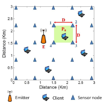
Figure 1: Problem geometry to be studied. The sensor layout defines a square grid, with each square having side $D$. Computations are made for the square shown shaded, with sensors 1, 2, 3 and 4. Interpolation methods are applied to points inside the square to estimate received power from the emitter at location $E$.

For the sake of concreteness, we postulate a particular geometry, as shown in Fig. 1. In a 3-km x 3-km area, a grid of sensors are superimposed where the sensors are separated by distance $D=640$ m. The postulated geometry is a typical coverage area that might be used, e.g., in a cellular network with a primary emitter (base station), primary clients and secondary emitters. We will use this geometry to quantify the accuracy of specific approaches. The proposed approaches can be scaled to other dimensions and extended to other geometries. Towards the objective of building a radio map, we focus on one of the sensor squares, shown by the shaded region in Fig. 1, and can apply our methodology to each square within the large grid. We will compute the RMS interpolation error at points inside the square by averaging over the statistical ensemble of shadow fading; we can also regard this as spatial averaging over all the squares in the grid, assuming the propagation model is statistically stationary. We assume that there is an emitter $E$ external to this square area and all given sensors (here, $n=4$) scans the same band, where each of the sensors measures and reports the received power from $E$. We assume the sensor measurements are sufficiently wideband that the effects of local multipath fading are averaged out. We continue to assume that the emitter location is known; later, however, we discuss how the case of unknown location and/or multiple emitters might be handled.

TABLE II: Simulation parameters

Parameter	Value
Path loss model	$15.3+10(3.76)\log_{10}d$
(3GPP suggested model[41])	$A=15.3,\gamma=3.76$
Shadow fading spread	$\sigma=5$ dB
Number of sensors	$n=4$
Length of a side of the square	$D=640$ m
Assumed coordinates for $n$ sensor	$(0,0),(0,640),(640,640),(640,0)$

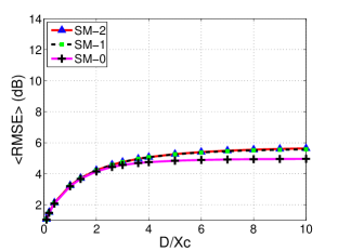
(a) Comparisons of SM-0, SM-1, SM-2

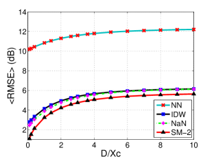
(b) Comparisons of SM-2 with Nearest Neighbor (NN), Natural Neighbor (NaN), Inverse Distance Weights (IDW)

Figure 2: Spatial averages over the square of RMS interpolation error, for different methods, as a function of $D/X_{c}$. Exponential correlation function, $\sigma=5$ dB and Emitter at $E(-100,0)$.

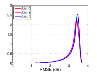
(a) Probability distribution function

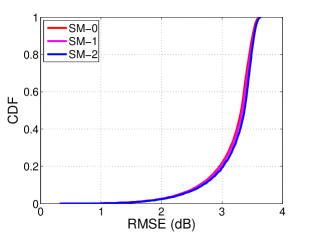
(b) Cumulative distribution function

Figure 3: Spatial distributions of RMS interpolation error over the square, for the SM family and $D/X_{c}=1$. Exponential correlation function, $\sigma=5$ dB and Emitter at $E(-100,0)$.

Here the impact of emitter $E$ at any arbitrary point $0$ is determined by collecting measurements at the $n=4$ sensors surrounding point $0$ and applying the proposed interpolation algorithms - SM-0, SM-1, and SM-2. We evaluate the performance of each algorithm with respect to RMS error as described in previous sections. Further, we provide a comparison of our proposed algorithms with several common interpolation techniques: Nearest Neighbor (NN), Inverse Distance Weighting (IDW), and Natural Neighbor (NaN). NN is the simplest interpolation technique where estimation at the point $0$ is equal to the measurement at the sensor nearest to point $0$. Both IDW and NaN provide estimates that are weighted sums of the $n$ sensor measurements, with the sum of the weights being 1. For IDW, each weight is based on distance to the sensor; for NaN, the weights are based on areas, using Voronoi cells[22].

Point 0 can be anywhere inside the square, and we will find the RMS interpolation error at many such points, specifically, points on a 64 $\times$ 64 array distributed uniformly over the square. At every one of the 64 $\times$ 64 = 4096 points, we will obtain the RMS interpolation error by averaging over 10000 realizations (or ‘instances’) of $[S_{0},S_{1},S_{2},S_{3},S_{4}]$; and then we will average over the square. The overall spatial average will be represented by the metric $<$RMSE$>$,

$$<\mbox{{RMSE}}>=\sqrt{\frac{\sum_{j=1}^{m}x_{j}^{2}}{m}},$$ (22)

where $<>$ in this case denotes a spatial average, and $x_{j}$ is the RMS error at the $j$-th point in the $64\times 64$ array. Other simulation parameters are listed in Table II.

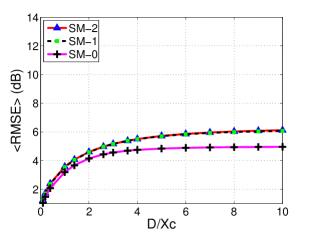
(a) RMSE for SM-0, SM-1, SM-2 when $E(-100,320)$

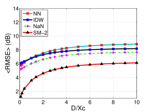
(b) RMSE comparison of SM-2 with NN, NaN, IDW $E(-100,320)$

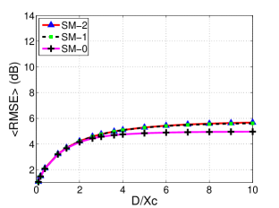
(c) RMSE for SM-0, SM-1, SM-2 when $E(-400,-400)$

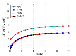
(d) RMSE comparison of SM-2 with NN, NaN, IDW $E(-400,-400)$

Figure 4: Effect of emitter location on $<$RMSE$>$ vs. $D/X_{c}$. Exponential correlation function and $\sigma=5$ dB.

VI-B Effect of Sensor Spacing

The most important parameter of the sensor network design is the sensor density, e.g., the number of sensors per unit area. This can also be captured by the nominal spacing between sensors which, in our problem geometry, Fig. 1, corresponds to the side of the square, $D$.

Moreover, the impact of the spacing depends, not on its absolute value, but on that value relative to the distance over which shadow fading decorrelates. From (4) (or related correlation functions), we can use the correlation distance $X_{c}$ for this purpose, and examine $<$RMSE$>$ as a function of $D/X_{c}$. Typically, $X_{c}$ varies from several meters to a few hundred meters, depending on the type of terrain [35, 22].

Fig. 2 shows $<$RMSE$>$ as a function of $D/X_{c}$ when the emitter is located at $E(-100,0)$ with respect to given sensor coordinates (see Table II). Fig. 2(a) compares $<$RMSE$>$ for proposed approaches SM-0, SM-1, and SM-2. As expected, SM-0 provides the lower bound of the estimation error. We note that error curves of SM-1 overlaps with SM-2, even though SM-2 lacks knowledge of the spatial correlation function. Furthermore, Fig. 2(b) shows that SM-2 estimates received power with the lowest RMS error when compared with the NN, IDW and NaN methods.

To affirm that $<$RMSE$>$ is an appropriate metric, we computed the probability density function (pdf) and its associated cumulative distribution function (CDF) over the $m=$ 4096 array points within the square. Results are shown in Fig. 3 for the particular case $D/X_{c}=$ 1. The major finding is the same for other values of $D/X_{c}$ as well, namely, that the RMS error is fairly uniform over the square. From the figure, for example, we observe for $D/X_{c}=$ 1 and the three SM approaches, that the RMS error is within 0.3 dB of $<$RMSE$>$ at 80$\%$ of the points in the array.

VI-C Effect of Emitter Location

For the family of SM approaches, the location of the emitter does not affect the estimate of $S_{0}$ but can affect the accuracy in estimating the median, $P_{m}$, at a given point. To demonstrate this impact, Fig. 4 shows plots of $<$RMSE$>$ vs. $D/X_{c}$ for two distinct locations. For the three SM approaches, the impact of emitter location is seen to be relatively small (see 4(a) and 4(c)); comparing 4(b) and 4(d), we see that the impact on NN, NaN and IDW is greater. These trends are evident across a range of emitter locations.

VI-D Effect of Correlation Function

The shape of the spatial correlation function in (4) is exponential, but other shapes may prevail, depending on the topography. To show the robustness of RMS error results to this shape, we now consider two other cases$-$

VI-D1 Gaussian correlation function

We now consider the correlation function[42]

$$c_{ab}=\sigma^{2}\exp\left[-\left(\frac{d_{ab}}{X_{c}}\right)^{2}\right]$$ (23)

Comparing Figs. 5(a) and 5(b) with Figs. 2(a) and 2(b), we see no substantial difference between the exponential and Gaussian correlation functions, (4) and (23).These functions can be considered circular, i.e., in each case, the locus of constant correlation is a circle. We next consider a correlation function that depends on direction as well as distance separation.

VI-D2 Elliptical correlation function

In this case, the locus of constant correlation is an ellipse, tilted at some rotation angle and having unequal major and minor axes. For one possible case, with a major-to-minor axis ratio of 3.3, we repeated the computations and obtained the results in Figs. 5(c) and 5(d). Again, we see no dramatic departure from results for other correlation functions.

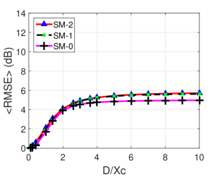
(a) RMSE for SM-0, SM-1, SM-2 for Gaussian correlation function

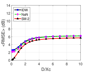
(b) RMSE comparison of SM-2 with NaN, IDW for Gaussian correlation function

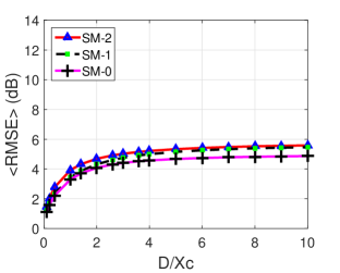
(c) RMSE for SM-0, SM-1, SM-2 for elliptical correlation function

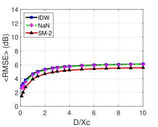
(d) RMSE comparison of SM-2 with NaN, IDW for elliptical correlation function

Figure 5: Effect of spatial correlation function on $<$RMSE$>$ vs. $D/X_{c}$. $\sigma=5$ dB and emitter at $E(-100,0)$.

VII Discussion

This section summarizes the major findings of our study through the analytical and graphical results for a square layout of sensors. We note that these findings can be generalized and scaled to other geometric configurations.

• The ideal stochastic method (SM-0) is identical to Simple Kriging and gives the lower bound on $<$RMSE$>$ as a function of $D/X_{c}$. The curve of $<$RMSE$>$ vs. $D/X_{c}$ rises smoothly from (0, 0) and approaches an asymptotic value equal to $\sigma$. This error curve is independent of emitter location.

• A key attribute of SM-0, SM-1 and SM-2 is that they estimate the parameters of the median received power, a consequence of which is that the RMS errors go to 0 as $D/X_{c}$ goes to 0.

• The RMS error curves for SM-1 and SM-2 are indistinguishable from each other in all cases; thus, using the nonparametric weighting method of SM-2 incurs virtually no penalty. For large $D/X_{c}$, the errors are slightly higher than for SM-0; the gap depends on the geometry of the emitter location, but is never more than about 0.2$\sigma$ (1 dB for $\sigma=5$ dB).

• IDW is computationally simpler than NaN, but NaN yields smaller RMS errors. However, the error curves for NaN and IDW do not approach 0 as $D/X_{c}$ approaches 0, in contrast to the SM cases. For both methods, the error curves are always above those for SM-2.

• The NN method is an outlier in this field of comparison. While simpler than all others, it is highly sensitive to emitter location and in some cases produces very large RMS errors compared to all others.

• SM-2 is much simpler to implement than NaN and Ideal Kriging (SM-0), and unlike the latter, requires no knowledge of the spatial correlation function. It also provides RMS errors that are fairly uniform across the coverage error.

• The behavior of the SM family of interpolation schemes is consistently better than IDW, NaN and NN for different spatial correlation functions.

Taken together, it appears that SM-2 provides the best tradeoff in terms of computational simplicity, RMSE performance, and robustness to emitter location, correlation function, and other network/environment conditions.

VIII Conclusion

The construction of a radio map based on interpolation from a sparsely deployed set of distributed sensors is a promising technique for monitoring spectrum usage. The utility of such a radio map can be extended to applications such as spectrum policing, network planning and management. The currently available two weighted-sum methods, IDW and NaN, have an important ‘robustness’ attribute in addition to not requiring knowledge of the spatial correlation function: They also do not require knowledge of the emitter location, or even knowledge of how many emitters are active; for each method, the operation is independent of this information. In the case of a single emitter of known location, the proposed stochastic methods (SM) can estimate path loss parameters to gain an advantage, and the result has been shown to be lower RMS errors in interpolating radio power. Notably, the practical approach SM-2 has low error in comparison with NaN and IDW when $D/X_{c}$ ranges between 0 and 1 and has consistent RMS error irrespective of the emitter location. For the most part, however, either IDW or NaN can be used as backup interpolation methods whenever the single-emitter location, or number of emitters, is unknown. The opportunities suggested by this observation are worthy of further study.

Acknowledgements: This material is based upon work supported by the National Science Foundation under ECCS-1247864 and CIF-1526908.

-A Equivalence of SM-0 and Kriging

Kriging is a spatially optimal linear predictor that involves weighted averaging of samples to arrive at an estimate. Weights for Kriging are chosen according to the best linear unbiased estimator (BLUE), which yields weights that depend upon the locations of sensors used in the prediction process and on the covariannce among them. Kriging is widely studied and reported in the literature [43, 44, 7, 12, 27] for different interpolation applications, and there are three main variations in the literature: (1) Simple Kriging, (2) Ordinary Kriging, and (3) Universal Kriging.

In our application, for the ideal case with known $A$ and $\gamma$, we will consider simple Kriging, for which the mean of the random process is assumed to be known. The optimal received power estimation at arbitrary point $0$, $Z^{*}(P_{r,0})$, is given by

$$Z^{*}(P_{r,0})=\bm{c_{0}^{T}C_{n}^{-1}P_{r}}+(1-\bm{c_{0}^{T}C_{n}^{-1}1})\mu,$$ (24)

which parallels eq. (7) in Cressie’s tutorial paper, [7], with the following notational changes: The arbitrary point $s_{0}$ (point 0 in this paper) in eq. (7) of [7] is replaced by $P_{r,0}$, the received power being estimated at that point; $\bm{c}’$ is replaced by $\bm{c_{0}^{T}}$; $\bm{C}$ is replaced by $\bm{C_{n}}$; and $\bm{Z}$ is replaced by $\bm{P_{r}}$, which is an $n\times 1$ vector of the powers measured at sensors $1,2,..,n$. In addition, Cressie’s formulation assumes a bias term, $\mu$, which is uniform throughout space, while our ‘bias’ term is the median path loss (of the form $A+10\gamma\log(d_{i})$), which differs at every point $i$. To accommodate this difference, we can rewrite (24) as follows:

$$Z^{*}(P_{r,0})=\bm{c_{0}^{T}C_{n}^{-1}P_{r}}+(P_{m,0}-\bm{c_{0}^{T}C_{n}^{-1}P_{m}}),$$ (25)

where $P_{m,0}$ is the median received power at point $0$; and $\bm{P_{m}}$ is an $n\times 1$ vector of the median powers at sensors $1,2,..n$.

Since $\bm{P_{r}}=\bm{P_{m}}+\bm{S}$, straightforward expansion of (25) yields

$$Z^{*}(P_{r,0})=P_{m,0}+\bm{c_{0}^{T}C_{n}^{-1}S}.$$ (26)

From eqs. (6) and (8) in the current paper, we see that this estimate differs from the true value of $P_{r,0}$ by just $\sigma_{0}u$. Thus, the mean-square error is $\sigma_{0}^{2}$, (8), just as in our analysis of SM-0. We conclude that Simple Kriging and SM-0 yield equivalent (and minimum) results for mean-square estimation error.

-B Estimation of $A$ and $\gamma$

To estimate values $A^{"}$ and $\gamma$ in (10), Least-Square Estimation (LSE) assumes functional approximations as

$$\bm{P}^{{}^{\prime}}=A^{{}^{\prime}}+10\gamma^{{}^{\prime}}\log_{10}\bm{d}$$ (27)

where $\bm{P}^{{}^{\prime}}$ is estimated received power vector of $P_{1}^{{}^{\prime}},..,P_{n}^{{}^{\prime}}$; and estimated values $A^{{}^{\prime}}$ and $\gamma^{{}^{\prime}}$ minimize the squared distance of $\|\bm{P}-\bm{P}^{{}^{\prime}}\|$ where $\bm{P}$ is a vector of $P_{1},..,P_{n}$.

Using LSE, solving for $A^{{}^{\prime}}$ and $\gamma^{{}^{\prime}}$ and using expression $P_{i}=A"+10\gamma\log d_{i}+S_{i}^{"}$, we get

$$\Delta\gamma= \gamma-\gamma^{{}^{\prime}}=\frac{\sum_{i=1}^{n}S_{i}\log\frac{\prod_{j=1}^{n}d_{j}}{d_{i}^{n}}}{10n\sum_{i=1}^{n}(\log d_{i})^{2}-10(\log\prod_{i=1}^{n}d_{i})^{2}},$$ (28)

$$\Delta A= A-A^{{}^{\prime}}$$

$$= \frac{\sum_{i=1}^{n}S_{i}\left(\log d_{i}(\prod_{j=1}^{n}d_{j})-\sum_{j=1}^{n}(\log d_{j})^{2}\right)}{n\sum_{i=1}^{n}(\log d_{i})^{2}-(\log\prod_{i=1}^{n}d_{i})^{2}},$$

where both $\Delta A$ and $\Delta\gamma$ are a linear sum of shadow fading at the sensor with constant coefficient terms that are functions of distance, $d_{i}$, between emitter and sensor $i$.

References

- [1] O. Ileri and N. B. Mandayam, “Dynamic spectrum access models: toward an engineering perspective in the spectrum debate,” Communications Magazine, IEEE, vol. 46, no. 1, pp. 153–160, January 2008.
- [2] Google, “Google spectrum database,” link: https://www.google.com/get/spectrumdatabase/.
- [3] Microsoft, “Microsoft spectrum observatory,” link: https://observatory.microsoftspectrum.com/.
- [4] I. Ziskind and M. Wax, “Maximum likelihood localization of multiple sources by alternating projection,” Acoustics, Speech and Signal Processing, IEEE Transactions on, vol. 36, no. 10, pp. 1553–1560, Oct 1988.
- [5] P. Misra and P. Enge, “Global positioning system: Signals, measurements and performance,” 2011, ganga-Jamuna Press.
- [6] K. Langendoen and N. Reijers, “Distributed localization in wireless sensor networks: A quantitative comparison,” Comput. Netw., vol. 43, no. 4, pp. 499–518, Nov. 2003. [Online]. Available: http://dx.doi.org/10.1016/S1389-1286(03)00356-6
- [7] N. Cressie, “The origins of kriging,” Mathematical Geology, vol. 22, no. 3, pp. 239–252, 1990. [Online]. Available: http://dx.doi.org/10.1007/BF00889887
- [8] J. Robinson, R. Swaminathan, and E. W. Knightly, “Assessment of urban-scale wireless networks with a small number of measurements,” in Proceedings of the 14th ACM International Conference on Mobile Computing and Networking, ser. MobiCom ’08. New York, NY, USA: ACM, 2008, pp. 187–198. [Online]. Available: http://doi.acm.org/10.1145/1409944.1409967
- [9] P. Agrawal and N. Patwari, “Correlated link shadow fading in multi-hop wireless networks,” Wireless Communications, IEEE Transactions on, vol. 8, no. 8, pp. 4024–4036, August 2009.
- [10] J. Wilson and N. Patwari, “Radio tomographic imaging with wireless networks,” Mobile Computing, IEEE Transactions on, vol. 9, no. 5, pp. 621–632, May 2010.
- [11] Y. Zhao, L. Morales, J. Gaeddert, K. Bae, J.-S. Um, and J. Reed, “Applying radio environment maps to cognitive wireless regional area networks,” in New Frontiers in Dynamic Spectrum Access Networks, 2007. DySPAN 2007. 2nd IEEE International Symposium on, April 2007, pp. 115–118.
- [12] A. Alaya-Feki, S. Ben Jemaa, B. Sayrac, P. Houze, and E. Moulines, “Informed spectrum usage in cognitive radio networks: Interference cartography,” in Personal, Indoor and Mobile Radio Communications, 2008. PIMRC 2008. IEEE 19th International Symposium on, Sept 2008, pp. 1–5.
- [13] G. Mateos, J.-A. Bazerque, and G. Giannakis, “Spline-based spectrum cartography for cognitive radios,” in Signals, Systems and Computers, 2009 Conference Record of the Forty-Third Asilomar Conference on, Nov 2009, pp. 1025–1029.
- [14] R. Dwarakanath, J. Naranjo, and A. Ravanshid, “Modeling of interference maps for licensed shared access in lte-advanced networks supporting carrier aggregation,” in Wireless Days (WD), 2013 IFIP, Nov 2013, pp. 1–6.
- [15] A. Garnaev, W. Trappe, and C.-T. Kung, “Optimizing scanning strategies: Selecting scanning bandwidth in adversarial rf environments,” in Cognitive Radio Oriented Wireless Networks (CROWNCOM), 2013 8th International Conference on, July 2013, pp. 148–153.
- [16] F. Digham, M.-S. Alouini, and M. K. Simon, “On the energy detection of unknown signals over fading channels,” in Communications, 2003. ICC ’03. IEEE International Conference on, vol. 5, May 2003, pp. 3575–3579 vol.5.
- [17] S. Liu, Y. Chen, W. Trappe, and L. Greenstein, “Aldo: An anomaly detection framework for dynamic spectrum access networks,” in INFOCOM 2009, IEEE, April 2009, pp. 675–683.
- [18] E. Visotsky, S. Kuffner, and R. Peterson, “On collaborative detection of tv transmissions in support of dynamic spectrum sharing,” in New Frontiers in Dynamic Spectrum Access Networks, 2005. DySPAN 2005. 2005 First IEEE International Symposium on, Nov 2005, pp. 338–345.
- [19] C. Phillips, D. Sicker, and D. Grunwald, “A survey of wireless path loss prediction and coverage mapping methods,” Communications Surveys Tutorials, IEEE, vol. 15, no. 1, pp. 255–270, First 2013.
- [20] ——, “Bounding the error of path loss models,” in New Frontiers in Dynamic Spectrum Access Networks (DySPAN), 2011 IEEE Symposium on, May 2011, pp. 71–82.
- [21] E. Dall’Anese, S.-J. Kim, and G. Giannakis, “Channel gain map tracking via distributed kriging,” Vehicular Technology, IEEE Transactions on, vol. 60, no. 3, pp. 1205–1211, March 2011.
- [22] S. Ureten, A. Yongacoglu, and E. Petriu, “A comparison of interference cartography generation techniques in cognitive radio networks,” in Communications (ICC), 2012 IEEE International Conference on, June 2012, pp. 1879–1883.
- [23] J. Bazerque, G. Mateos, and G. Giannakis, “Group-lasso on splines for spectrum cartography,” Signal Processing, IEEE Transactions on, vol. 59, no. 10, pp. 4648–4663, Oct 2011.
- [24] ——, “Basis pursuit for spectrum cartography,” in Acoustics, Speech and Signal Processing (ICASSP), 2011 IEEE International Conference on, May 2011, pp. 2992–2995.
- [25] L. Bolea, J. Perez-Romero, and R. Agusti, “Received signal interpolation for context discovery in cognitive radio,” in Wireless Personal Multimedia Communications (WPMC), 2011 14th International Symposium on, Oct 2011, pp. 1–5.
- [26] H. Ledoux and C. Gold, “An efficient natural neighbour interpolation algorithm for geoscientific modelling,” in Developments in Spatial Data Handling. Springer Berlin Heidelberg, 2005, pp. 97–108. [Online]. Available: http://dx.doi.org/10.1007/3-540-26772-7_8
- [27] M. Angjelicinoski, V. Atanasovski, and L. Gavrilovska, “Comparative analysis of spatial interpolation methods for creating radio environment maps,” in Telecommunications Forum (TELFOR), 2011 19th, Nov 2011, pp. 334–337.
- [28] M. Hata, “Empirical formula for propagation loss in land mobile radio services,” Vehicular Technology, IEEE Transactions on, vol. 29, no. 3, pp. 317–325, Aug 1980.
- [29] V. Erceg, L. Greenstein, S. Tjandra, S. Parkoff, A. Gupta, B. Kulic, A. Julius, and R. Bianchi, “An empirically based path loss model for wireless channels in suburban environments,” Selected Areas in Communications, IEEE Journal on, vol. 17, no. 7, pp. 1205–1211, Jul 1999.
- [30] T. S. Rappaport, “Wireless communications: principles and practice,” Ch. 3.9, Vol. 2, Prentice Hall PTR, 1996.
- [31] A. Goldsmith, “Wireless communications,” Ch. 2.6, Cambridge University Press, 2005.
- [32] P. J. Bickel and K. A. Doksum, “Mathematical statistics : basic ideas and selected topics, volume I,” Ch. 2, 2nd ed., Prentice Hall, 2001.
- [33] J. A. Rice, “Mathematical statistics and data analysis,” Ch. 8 and 14, 2nd ed., Duxbury Press, 1995.
- [34] M. Gudmundson, “Correlation model for shadow fading in mobile radio systems,” Electronics Letters, vol. 27, no. 23, pp. 2145–2146, Nov 1991.
- [35] A. Goldsmith, L. Greenstein, and G. Foschini, “Error statistics of real-time power measurements in cellular channels with multipath and shadowing,” Vehicular Technology, IEEE Transactions on, vol. 43, no. 3, pp. 439–446, Aug 1994.
- [36] X. Zhao, L. Razouniov, and L. Greenstein, “Path loss estimation algorithms and results for rf sensor networks,” in Vehicular Technology Conference, 2004. VTC2004-Fall. 2004 IEEE 60th, vol. 7, Sept 2004, pp. 4593–4596 Vol. 7.
- [37] N. Cressie, “Statistics for spatial data,” Terra Nova, vol. 4, no. 5, pp. 613–617, 1992. [Online]. Available: http://dx.doi.org/10.1111/j.1365-3121.1992.tb00605.x
- [38] R. D. Yates and D. J. Goodman, Probability and stochastic processes. John Wiley and Sons, 1999.
- [39] M. L. Eaton, Multivariate Statistics: a Vector Space Approach. John Wiley and Sons, 1983.
- [40] M. Osborne, “Least squares and maximum likelihood.”
- [41] G. T. Report, “TR 36.814 V9.0.0 (2010-03).”
- [42] P. Abrahamsen, A Review of Gaussian Random Fields and Correlation Functions. Norsk Regnesentral/Norwegian Computing Center, 1997. [Online]. Available: https://books.google.com/books?id=InByAAAACAAJ
- [43] S. R. X. Ying and R. Poovendran, “Incentivizing crowdsourcing for radio environment mapping with statistical interpolation,” 2015, IEEE DySPAN.
- [44] C.-W. K. X. Ying and S. Roy, “Revisiting tv coverage estimation with measurement-based statistical interpolation,” 2015, IEEE COMSNeTs.