Radiative decays of $1^{++}$ heavy mesons in the covariant light-front approach

Abstract

We calculate the predicted width for the radiative decay of a $1^{++}$ heavy meson via the channel $1^{++}\to 1^{--}+\gamma$ in the covariant light-front quark model. Specifically, we compute the decay widths for $\chi_{c1}(1P)\to J/\psi+\gamma$ and $\chi_{b1}(nP)\to\Upsilon(n^{\prime}S)+\gamma$. The results are compared with experimental data and with predictions from calculations based on nonrelativistic models and their extensions to include relativistic effects.

I Introduction

Experimental observations and theoretical studies of heavy quarkonium $Q\bar{Q}$ states have played a very valuable role in elucidating the properties of quantum chromodynamics (QCD). A heavy quark is one whose mass, $m_{Q}$, is large compared with $\Lambda_{QCD}\sim 0.3$, so that the running QCD coupling $g_{s}(M_{Q})$ and the associated quantity $\alpha_{s}(m_{Q})=g_{s}(M_{Q})^{2}/(4\pi)$ are reasonably small, allowing perturbative treatments of at least some parts of the physics of $Q\bar{Q}$ states and decays. Furthermore, for $m_{Q}\gg\Lambda_{QCD}$, one can obtain an approximate description of many properties of the $Q\bar{Q}$ states using nonrelativistic methods, including potential models. From the time of the discovery of the $J/\psi$ at BNL Aubert:1974js and SLAC/SPEAR psi_slac in 1974, and the $\Upsilon$ at Fermilab in 1977 Herb:1977ek ; Innes:1977ae , there has been a steadily growing wealth of data on the various $Q\bar{Q}$ states, where the $Q$ denotes a charm quark $c$ or a bottom/beauty quark $b$, as well as data on mesons and baryons with charm and bottom/beauty quantum numbers. Some reviews of heavy quarkonia and references to the literature include quiggrosner79 -rosner2013 .

These experimental achievements motivate the continued theoretical study of the structure and properties of $c\bar{c}$ and $b\bar{b}$ quarkonium states. Among quarkonium decays, radiative decays are particularly valuable as tests of various models, since the photon is directly observed and the nature of the electromagnetic transition is well understood. One of the simplest types of radiative decays is the electric dipole (E1) transition between a $Q\bar{Q}$ state with radial quantum number $n$ and spectroscopic type $n\,{}^{2S+1}\,L_{J}=n{}^{3}\,L_{J}$ with $L=1$ (P-wave) and $J=0,\ 1,\ 2$, denoted $\chi_{QJ}(nP)$ in standard notation, where $Q=c,\ b$, and a lower-lying $Q\bar{Q}$ S-wave state $n^{\prime}\,{}^{3}S_{1}$, in particular, $J/\psi$ and $\psi(2S)$ for the $c\bar{c}$ system, and $\Upsilon(n^{\prime}S)$ with $n^{\prime}=1,\ 2,\ 3$ for the $b\bar{b}$ system. In terms of $J^{PC}$ values, these decays are of the form $J^{++}\to 1^{--}+\gamma$, where $J=0,\ 1,\ 2$. The P-wave $c\bar{c}$ states were first observed in 1976 by the SLAC-LBL experiment at SLAC/SPEAR Whitaker:1976hb ; Biddick:1977sv . The P-wave $b\bar{b}$ states were first observed by the Columbia-Stony Brook (CUSB) experiment at the Cornell CESR $e^{+}e^{-}$ storage ring klopfenstein83 ; pauss83 and confirmed by the CLEO experiment at CESR haas84 . Larger data samples and quite accurate measurements of branching ratios for radiative decays of P-wave $b\bar{b}$ states were obtained later, in particular, by the CLEO III kornicer2011 and BABAR experiments babar2014 . Valuable results have also been obtained from hadron colliders, including the observation of the $\chi_{bJ}(3P)$ $b\bar{b}$ states at the Large Hadron Collider (LHC) Aad:2011ih and the measurement of the mass of $\chi_{b1}(3P)$ by LHCb Aaij:2014hla .

There have been a number of theoretical studies of these E1 transitions based on a range of different models Karl:1980wm -Brambilla:2005zw . Many of these models make use of nonrelativistic potentials, such as the potential $V=-(4/3)\alpha_{s}(m_{Q})/r+\sigma r$, where the first term is a non-Abelian Coulomb potential representing one-gluon exchange at short distances and the second term is the linear confining potential, with $\sigma$ denoting the string tension. These are reasonable models, since a $Q\bar{Q}$ bound-state system is nonrelativistic if $m_{Q}/\Lambda_{QCD}\gg 1$.

It is of interest to investigate these radiative decays of P-wave quarkonium states using a different type of model, namely the light-front quark model (LFQM)Terentev:1976jk -Cheng:2003sm . This approach permits a fully relativistic treatment of the quark spins and the internal motion of the constituent quarks. In this covariant approach, the hadronic structure for small momentum transfer is represented by one-loop diagrams evaluated on the light cone. It has been used to study semileptonic and nonleptonic decays of heavy-flavor $D$ and $B$ mesons and also to evaluate radiative decay rates of heavy mesons Hwang:2006cua ; Choi:2007se ; Hwang:2010iq ; Ke:2010vn ; Ke:2013zs . In particular, in Ke:2013zs with Ke and Li, we used this approach to calculate the widths for the radiative decays of heavy $0^{++}$ and $1^{+-}$ $Q\bar{Q}$ mesons.

In the light-front formalism, one chooses the coordinate where $q^{+}=0$, in which the quark current cannot create or annihilate pairs, and the relevant transition matrix element can be computed as an overlap of Fock-space wavefunctions. The terms involving pair production or annihilation vanish Drell:1969km ; Brodsky:1997de . An advantage of the light-front quark model is that it is manifestly covariant. In the light-front approach, it is easy to boost a hadron bound states from one inertial Lorentz frame to another one when the bound state wavefunction is known in a particular frameBrodsky:1997de .

In this paper, extending our previous work with Ke and Li in Ref. Ke:2013zs , we study the radiative decays

$$\chi_{c1}(1P)\to J/\psi+\gamma$$ (1)

and

$$\chi_{b1}(nP)\to\Upsilon(n^{\prime}S)+\gamma$$ (2)

where $n\geq n^{\prime}$ by using the light-front quark model. With the front-front formalism, we perform a numerical calculation the widths for these decays and then compare the results with theoretical calculations based on other approaches.

The paper is organized as follows: In Section II, we derive the formulas for the radiative decay $1^{++}\to 1^{--}+\gamma$. Then in section III, we discuss the meson wavefunctions that are relevant to the light-front approach. In Section IV, we discuss numerical results for the decay widths of $\chi_{c1}(1P)\to J/\psi+\gamma$ and $\chi_{b1}(nP)\to\Upsilon(n^{\prime}S)+\gamma$. Our conclusions are given in Section V.

II Light-front formalism for the decays $1^{++}\to 1^{--}+\gamma$

II.1 Notation

Here we briefly summarize the notation that is relevant for radiative transition of meson. We follow the covariant light-front approach of Jaus:1999zv ; Cheng:2003sm and use the same notation. In light-front coordinates, a (four-)momentum $p$ is expressed as

$$p^{\mu}=(p^{-},p^{+},{\vec{p}}_{\perp})$$ (3)

where

$$p^{+}=p^{0}+p^{3},\quad p^{-}=p^{0}-p^{3}$$ (4)

and

$${\vec{p}}_{\perp}=(p^{1},p^{2})\ .$$ (5)

Thus,

$$p^{2} = (p^{0})^{2}-|\vec{p}|^{2}=(p^{0})^{2}-(p^{3})^{2}-|{\vec{p}}_{\perp}|^{2}$$ (6)

$$= p^{+}p^{-}-|{\vec{p}}_{\perp}|^{2}\ .$$ (8)

We denote the momentum of the parent (incoming) meson as $P^{\prime}=p^{\prime}_{1}+p_{2}$, where $p^{\prime}_{1}$ and $p_{2}$ are the momenta of the constituent quark and anti-quark, with mass $m^{\prime}_{1}$ and $m_{2}$, respectively. Similarly, we label the momentum of the daughter (outgoing) quarkonium meson as $P^{\prime\prime}=p^{\prime\prime}_{1}+p_{2}$, where $p^{\prime\prime}_{1}$ is the momentum of the constituent quark, with mass $m^{\prime\prime}_{1}$. For our application to $Q\bar{Q}$ quarkonium systems, $m^{\prime}_{1}=m_{2}=m^{\prime\prime}=m_{Q}$. The four-momentum of the parent meson with mass $M^{\prime}$, in terms of light-front coordinates, is

$$P^{\prime}=(P^{\prime-},P^{\prime+},{\vec{P}}^{\prime}_{\perp})$$ (9)

so $P^{\prime 2}=P^{\prime+}P^{\prime-}-|{\vec{P}}_{\perp}|^{2}=M^{\prime 2}$. Similarly, for the outgoing meson, $P^{\prime\prime 2}=M^{\prime\prime 2}$. In what follows, the vector signs on transverse momentum components are to be understood implicitly and are suppressed in the notation. The internal motion of the constituents can be described by the variables $(x_{2},p^{\prime}_{\perp})$, where

$$p^{\prime+}_{1}=x_{1}P^{\prime+},\quad p^{+}_{2}=x_{2}P^{\prime+}$$

$$p^{\prime}_{1\perp}=x_{1}P^{\prime}_{\perp}+p^{\prime}_{\perp},\quad p_{2\perp}=x_{2}P^{\prime}_{\perp}-p^{\prime}_{\perp}$$

$$x_{1}+x_{2}=1$$ (10)

and $p^{\prime\prime}_{\perp}$ can be expressed as

$$p^{\prime\prime}_{\perp}=p^{\prime}_{\perp}-x_{2}q_{\perp}.$$ (11)

II.2 Form factors

Let us define $P=P^{\prime}+P^{\prime\prime}$ and $q=P^{\prime}-P^{\prime\prime}$. Since the initial P-wave $1^{++}$ $Q\bar{Q}$ state is an axial-vector, we denote it as $A$, while the final $1^{--}$ $Q\bar{Q}$ state is a vector, denoted $V$. The general amplitude for the transition $A(1^{++})\to V(1^{--})+\gamma$ has the form

$$i{\cal A}\left(A(P^{\prime})\to V(P^{\prime\prime})\gamma(q)\right)=\varepsilon^{*}_{\mu}(q)\varepsilon^{\prime}_{\nu}(P^{\prime})\varepsilon^{\prime\prime*}_{\rho}(P^{\prime\prime})i\tilde{\cal A}^{\mu\nu\rho}\ ,$$ (12)

where $\varepsilon^{\prime}_{\nu}(P^{\prime})$, $\varepsilon^{\prime\prime*}_{\rho}(P^{\prime\prime})$, and $\varepsilon^{*}_{\mu}(q)$ are the polarization (four-)vectors of the parent heavy axial-vector meson, the daughter heavy vector meson, and the photon, respectively. The structure of this amplitude was given in Dudek:2006ej . We review this next. Since quantum electrodynamic (QED) interactions are invariant under parity and time reversal (and thus also CP), this amplitude must be P- and T-invariant. In addition to these two conditions, the transverse properties of the polarization vectors yield the three further conditions

$$\varepsilon^{\prime}_{\nu}(P^{\prime})(P+q)^{\nu}=0,$$ (13)

$$\varepsilon^{\prime\prime*}_{\rho}(P^{\prime\prime})(P-q)^{\rho}=0,$$ (14)

and

$$\varepsilon^{*}_{\mu}(q)q^{\mu}=0.$$ (15)

Condition (15) is also implied by electromagnetic gauge invariance. Applying these conditions, we obtain the following general amplitude (to be simplified below):

$$i\tilde{\cal A}^{\mu\nu\rho} = f_{1}\epsilon^{\mu\nu\rho\alpha}P_{\alpha}+f_{2}\epsilon^{\mu\nu\rho\alpha}q_{\alpha}+f_{3}\epsilon^{\rho\nu\alpha\beta}P^{\mu}P_{\alpha}q_{\beta}$$ (16)

$$+ f_{4}\epsilon^{\mu\nu\alpha\beta}P^{\rho}P_{\alpha}q_{\beta}+f_{5}\epsilon^{\rho\mu\alpha\beta}P^{\nu}P_{\alpha}q_{\beta}\ .$$

This expression can be simplified by using the fact that the photon only has two transverse polarization states, so the timelike component $\varepsilon^{*}_{0}(q)=0$. Taking the parent axial vector meson $A(P^{\prime})$ to be in its rest frame, we have $P^{\prime\mu}=(M^{\prime},0)$, where $M^{\prime}$ is mass of $A(P^{\prime})$. The $f_{3}$ term can be eliminated:

$$[f_{3}\epsilon^{\rho\nu\alpha\beta}P^{\mu}P_{\alpha}q_{\beta}]\varepsilon^{*}_{\mu}(q)\varepsilon^{\prime}_{\nu}(P^{\prime})\varepsilon^{\prime\prime*}_{\rho}(P^{\prime\prime})\propto\varepsilon^{*}_{\mu}(q)P^{\mu}$$

$$=2\varepsilon^{*}_{\mu}(q)P^{\prime\mu}=2\varepsilon^{*}_{0}(q)P^{\prime 0}=0\ .$$ (17)

Furthermore, the $f_{1}$ term vanishes due to electromagnetic gauge invariance, $q_{\mu}\tilde{A}^{\mu\nu\rho}=0$. Therefore, the general amplitude that satisfies the five conditions above is given by Dudek:2006ej :

$$i\tilde{\cal A}^{\mu\nu\rho}\to i{A}^{\mu\nu\rho}$$

$$=f_{2}\epsilon^{\mu\nu\rho\alpha}q_{\alpha}+f_{4}\epsilon^{\mu\nu\alpha\beta}P^{\rho}P_{\alpha}q_{\beta}+f_{5}\epsilon^{\rho\mu\alpha\beta}P^{\nu}P_{\alpha}q_{\beta}\ .$$

(18)

The $f_{2}$ term corresponds to the electric dipole (E1) transition and makes the dominant contribution to the amplitude, while the $f_{4}$ and $f_{5}$ terms correspond to the magnetic dipole (M2) transition and make subdominant contributions Cho:1994gb ; Shao:2012fs . A detailed analysis of parity and time-reversal invariance of this general amplitude is given in Appendix A.

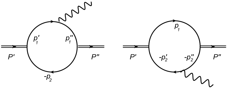
Figure 1: Feynman diagrams for radiative transitions in the light-front framework.

II.3 Calculation of radiative decay amplitude

In general, the width for an electromagnetic dipole transition between an initial $Q\bar{Q}$ state $n\,{}^{3}P_{J}$ and a final state $n^{\prime}\,{}^{3}S_{1}+\gamma$ is given by (e.g., kwong_rosner_quigg1987 )

$$\Gamma(n\,{}^{3}P_{J}\to n^{\prime}\,{}^{3}S_{1}+\gamma)=\frac{4\alpha_{em}e_{Q}^{2}E_{\gamma}^{3}}{9}\,|\langle f|{\vec{r}}|i\rangle|^{2}\ ,$$ (19)

where $e_{Q}$ is the quark of the quark $Q$, $E_{\gamma}$ is the energy of the outgoing photon in the parent rest frame, and $i$ and $j$ denote the initial- and final-state wavefunctions. For our calculation in the LFQM, we note that the vertex function for the parent axial-vector meson $A(1^{++})$ is given by Cheng:2003sm :

$$iH^{\prime}_{A}\left[\gamma^{\nu}+\frac{(p^{\prime}_{1}-p_{2})^{\nu}}{W^{\prime}_{A}}\right]\gamma^{5},$$ (20)

and the vertex function for the daughter vector meson $V(1^{--})$ is

$$iH^{\prime\prime}_{V}\left[\gamma^{\rho}-\frac{(p^{\prime\prime}_{1}-p_{2})^{\rho}}{W^{\prime\prime}_{V}}\right]\ ,$$ (21)

where $H^{\prime}_{A}$ and $H^{\prime\prime}_{V}$ are functions of $p^{\prime}_{1}$, $p^{\prime\prime}_{1}$ and $p_{2}$. The explicit forms for these vertex functions will be discussed below.

There are two diagrams that contribute at leading order to the $A\to V+\gamma$ transition amplitude, so we write

$$i{\cal A}^{\mu\nu\rho}(A\to V+\gamma)=i{\cal A}^{\mu\nu\rho}(a)+i{\cal A}^{\mu\nu\rho}(b)\ ,$$ (22)

where the left-hand diagram in Fig.(1) corresponds to ${\cal A}^{\mu\nu\rho}(a)$ and the right-hand diagram in Fig.(1) corresponds to ${\cal A}^{\mu\nu\rho}(b)$. These are related by charge conjugation. For the left-hand diagram, the transition amplitude is given by

$$i{\cal A}^{\mu\nu\rho}(a)=eN_{e1^{\prime}}\frac{N_{c}}{(2\pi)^{4}}\int d^{4}p^{\prime}_{1}\frac{H^{\prime}_{A}H^{\prime\prime}_{V}}{N^{\prime}_{1}N^{\prime\prime}_{1}N_{2}}{\cal S}^{\mu\nu\rho}_{a}\ ,$$ (23)

where

$${\cal S}^{\mu\nu\rho}_{a} = \text{Tr}\left\{(p/^{\prime\prime}_{1}+m^{\prime\prime}_{1})\gamma^{\mu}(p/_{1}^{\prime}+m^{\prime}_{1})[\gamma^{\nu}+\frac{(p^{\prime}_{1}-p_{2})^{\nu}}{W^{\prime}_{A}}]\right.$$ (24)

$$\times \left.\gamma^{5}(-p/_{2}+m_{2})[\gamma^{\rho}-\frac{1}{W^{\prime\prime}_{V}}(p^{\prime\prime}_{1}-p_{2})^{\rho}]\right\}$$

$$= -p^{\prime\prime\mu}_{1}\text{Tr}[p/^{\prime}_{1}\gamma^{\nu}p/_{2}\gamma^{\rho}\gamma^{5}]+(p^{\prime}_{1}\cdot p^{\prime\prime}_{1}-m^{\prime}_{1}m^{\prime\prime}_{1})$$

$$\times \text{Tr}[\gamma^{\mu}\gamma^{\nu}p/_{2}\gamma^{\rho}\gamma^{5}]-p^{\prime\mu}_{1}\text{Tr}[p/^{\prime\prime}_{1}\gamma^{\nu}p/_{2}\gamma^{\rho}\gamma^{5}]$$

$$- \frac{m^{\prime\prime}_{1}}{W^{\prime}_{A}}(p^{\prime}_{1}-p_{2})^{\nu}\text{Tr}[\gamma^{\mu}p/^{\prime}_{1}p/_{2}\gamma^{\rho}\gamma^{5}]-m^{\prime\prime}_{1}m_{2}$$

$$\times \text{Tr}[\gamma^{\mu}p/^{\prime}_{1}\gamma^{\nu}\gamma^{\rho}\gamma^{5}]-\frac{m^{\prime}_{1}}{W^{\prime}_{A}}(p^{\prime}_{1}-p_{2})^{\nu}\text{Tr}[p/^{\prime\prime}_{1}\gamma^{\mu}p/_{2}\gamma^{\rho}\gamma^{5}]$$

$$- m^{\prime}_{1}m_{2}\text{Tr}[p/^{\prime\prime}_{1}\gamma^{\mu}\gamma^{\nu}\gamma^{\rho}\gamma^{5}]-\frac{m^{\prime}_{1}}{W^{\prime\prime}_{V}}(p^{\prime\prime}_{1}-p_{2})^{\rho}$$

$$\times \text{Tr}[p/^{\prime\prime}_{1}\gamma^{\mu}\gamma^{\nu}p/_{2}\gamma^{5}]-\frac{m^{\prime\prime}_{1}}{W_{V}^{\prime\prime}}(p^{\prime\prime}_{1}-p_{2})^{\rho}\text{Tr}[\gamma^{\mu}p/^{\prime}_{1}\gamma^{\nu}p/_{2}\gamma^{5}]$$

$$- [\frac{(p^{\prime}_{1}-p_{2})^{\nu}}{W^{\prime}_{A}}m_{2}+p_{2}^{\nu}]\text{Tr}[p/^{\prime\prime}_{1}\gamma^{\mu}p/^{\prime}_{1}\gamma^{\rho}\gamma^{5}]$$

$$- [\frac{(p^{\prime}_{1}-p_{2})^{\nu}}{W^{\prime}_{A}}\frac{(p^{\prime\prime}_{1}-p_{2})^{\rho}}{W^{\prime\prime}_{V}}-g^{\rho\nu}]\text{Tr}[p/^{\prime\prime}_{1}\gamma^{\mu}p/^{\prime}_{1}p/_{2}\gamma^{5}]$$

$$- [p^{\rho}_{2}+\frac{m_{2}}{W^{\prime\prime}_{V}}(p^{\prime\prime}_{1}-p_{2})^{\rho}]\text{Tr}[p/^{\prime\prime}_{1}\gamma^{\mu}p/^{\prime}_{1}\gamma^{\nu}\gamma^{5}]\ ,$$

$$N^{\prime}_{1}=p^{\prime 2}_{1}-m^{\prime 2}_{1}+i\epsilon,$$ (25)

$$N^{\prime\prime}_{1}=p^{\prime\prime 2}_{1}-m^{\prime\prime 2}_{1}+i\epsilon,$$ (26)

$$N_{2}=p^{2}_{2}-m^{2}_{2}+i\epsilon,$$ (27)

and $N_{e1^{\prime}(e2)}$ denotes the electric charge of the constituent quark in units of $e$. The contribution to the amplitude from the right-hand diagram follows from this.

To calculate the amplitude in the covariant light-front approach, we need to integrate over the internal momentum, $p^{\prime-}_{1}$. In order to do this, we first express the amplitude in terms of internal momentum $p^{\prime}_{1}$ and external momenta $P$ and $q$, as well as $N^{\prime}_{1}$, $N^{\prime\prime}_{1}$, $N_{2}$, by using the following relations:

$$p^{\prime\prime}_{1} = p^{\prime}_{1}-q$$

$$p_{2} = (P+q)/2-p^{\prime}_{1}$$

$$2p^{\prime}_{1}\cdot p_{2} = M^{\prime 2}-N^{\prime}_{1}-m^{\prime 2}_{1}-N_{2}-m^{2}_{2}$$

$$2p^{\prime\prime}_{1}\cdot p_{2} = M^{\prime\prime 2}-N^{\prime\prime}_{1}-m^{\prime\prime 2}_{1}-N_{2}-m^{2}_{2}$$

$$2p^{\prime}_{1}\cdot p^{\prime\prime}_{1} = -q^{2}+N^{\prime}_{1}+m^{\prime 2}_{1}+N^{\prime\prime}_{1}+m^{\prime\prime 2}_{1}.$$ (28)

After the integration over $p^{\prime-}_{1}$, one makes the following replacement Jaus:1999zv ; Cheng:2003sm :

$$\int d^{4}p^{\prime}_{1}\frac{H^{\prime}_{A}H^{\prime\prime}_{V}}{N^{\prime}_{1}N^{\prime\prime}_{1}N_{2}}{\cal S}^{\mu\nu\rho}_{a}\varepsilon^{*}_{\mu}\varepsilon^{\prime}_{\nu}\varepsilon^{\prime\prime*}_{\rho}\to$$

$$-i\pi\int dx_{2}d^{2}p^{\prime}_{\perp}\frac{h^{\prime}_{A}h^{\prime\prime}_{V}}{x_{2}\hat{N}^{\prime}_{1}\hat{N}^{\prime\prime}_{1}}\hat{\cal S}^{\mu\nu\rho}_{a}\hat{\varepsilon}^{*}_{\mu}\hat{\varepsilon}^{\prime}_{\nu}\hat{\varepsilon}^{\prime\prime*}_{\rho}\ ,$$ (29)

where

$$N^{\prime}_{1}\to\hat{N}^{\prime}_{1}=x_{1}(M^{\prime 2}-M^{\prime 2}_{0})$$

$$N^{\prime\prime}_{1}\to\hat{N}^{\prime\prime}_{1}=x_{1}(M^{\prime\prime 2}-M^{\prime\prime 2}_{0})$$

$$H^{\prime}_{A}\to h^{\prime}_{A}=(M^{\prime 2}-M^{\prime 2}_{0})\sqrt{\frac{x_{1}x_{2}}{N_{c}}}\frac{\tilde{M}^{\prime}_{0}}{4M^{\prime}_{0}}\phi_{np}(x_{2},p^{\prime}_{\perp})$$

$$H^{\prime\prime}_{V}\to h^{\prime\prime}_{V}=(M^{\prime\prime 2}-M^{\prime\prime 2}_{0})\sqrt{\frac{x_{1}x_{2}}{N_{c}}}\frac{1}{\sqrt{2}\tilde{M}^{\prime\prime}_{0}}\phi_{n^{\prime}s}(x_{2},p^{\prime\prime}_{\perp})$$

$$W^{\prime}_{A}\to w^{\prime}_{A}=\frac{\tilde{M}^{\prime 2}_{0}}{m^{\prime}_{1}-m_{2}}$$

$$W^{\prime\prime}_{V}\to w^{\prime\prime}_{V}=M^{\prime\prime}_{0}+m^{\prime\prime}_{1}+m_{2}\ .$$ (30)

In the above expressions, $\phi_{n^{\prime}s}$ and $\phi_{np}$ represent the wavefunction for the S-wave $Q\bar{Q}$ meson $V$ and the P-wave $Q\bar{Q}$ meson $A$, respectively. We will discuss these wavefunctions in detail in the next section. The definitions of $M^{\prime}_{0}$, $M^{\prime\prime}_{0}$, $\tilde{M}^{\prime}_{0}$ and $\tilde{M}^{\prime\prime}_{0}$ are given in appendix C. The definition of $\hat{\varepsilon}^{*}$, $\hat{\varepsilon}^{\prime}$ and $\hat{\varepsilon}^{\prime\prime*}_{\rho}$ is given in Jaus:1999zv ; Cheng:2003sm .

One should also include the contribution from zero modes in the $A$ meson. In practice, this amounts to the following replacement for $p^{\prime}_{1\mu}$ in $\hat{\cal S}^{\mu\nu\rho}_{a}$ in the integral Jaus:1999zv ; Cheng:2003sm :

$$\hat{p}^{\prime}_{1\mu} \to P_{\mu}A^{(1)}_{1}+q_{\mu}A^{(1)}_{2}\ ,$$

$$\hat{p}^{\prime}_{1\mu}\hat{p}^{\prime}_{1\nu} \to g_{\mu\nu}A^{(2)}_{1}+P_{\mu}P_{\nu}A^{(2)}_{2}$$

$$+ (P_{\mu}q_{\nu}+q_{\mu}P_{\nu})A^{(2)}_{3}+q_{\mu}q_{\nu}A^{(2)}_{4}\ ,$$

$$\hat{p}^{\prime}_{1\mu}\hat{p}^{\prime}_{1\nu}\hat{p}^{\prime}_{1\alpha} \to (g_{\mu\nu}P_{\alpha}+g_{\mu\alpha}P_{\nu}+g_{\nu\alpha}P_{\mu})A^{(3)}_{1}$$ (31)

$$+ (g_{\mu\nu}q_{\alpha}+g_{\mu\alpha}q_{\nu}+g_{\nu\alpha}q_{\mu})A^{(3)}_{2}$$

$$+ P_{\mu}P_{\nu}P_{\alpha}A^{(3)}_{3}+(P_{\mu}P_{\nu}q_{\alpha}+P_{\mu}q_{\nu}P_{\alpha}$$

$$+ q_{\mu}P_{\nu}P_{\alpha})A^{(3)}_{4}+(q_{\mu}q_{\nu}P_{\alpha}+q_{\mu}P_{\nu}q_{\alpha}$$

$$+ P_{\mu}q_{\nu}q_{\alpha})A^{(3)}_{5}+q_{\mu}q_{\nu}q_{\alpha}A^{(3)}_{6}\ .$$

After these operations, the amplitude ${\cal A}^{\mu\nu\rho}(a)$ can be expressed as a function of the external four-momenta $P$ and $q$. It can be parametrized in the following form:

$$i{\cal A}^{\mu\nu\rho}(a) = f^{a}_{2}\epsilon^{\mu\nu\rho\alpha}q_{\alpha}+f^{a}_{4}\epsilon^{\mu\nu\alpha\beta}P^{\rho}P_{\alpha}q_{\beta}$$ (32)

$$+ f^{a}_{5}\epsilon^{\rho\mu\alpha\beta}P^{\nu}P_{\alpha}q_{\beta}\ ,$$

with

$$f^{a}_{2}(q^{2}) = eN_{e^{\prime}_{1}}\frac{N_{c}}{16\pi^{3}}\int dx_{2}d^{2}p^{\prime}_{\perp}\frac{h^{\prime}_{A}h^{\prime\prime}_{V}}{x_{2}\hat{N}^{\prime}_{1}\hat{N}^{\prime\prime}_{1}}(-4)\cdot\left[\frac{1}{w^{\prime}_{A}}(m^{\prime\prime}_{1}+m^{\prime}_{1}-2m_{2})A^{(2)}_{1}+\frac{1}{w^{\prime\prime}_{V}}(2m_{2}+m^{\prime}_{1}+m^{\prime\prime}_{1})A^{(2)}_{1}\right.$$

$$- \left.\frac{1}{4}(1-2A^{(1)}_{2})\left(-q^{2}+\hat{N}^{\prime}_{1}+\hat{N}^{\prime\prime}_{1}+(m^{\prime}_{1}-m^{\prime\prime}_{1})^{2}\right)-A^{(1)}_{2}(m^{\prime\prime}_{1}m_{2}-m^{\prime}_{1}m_{2})-m^{\prime}_{1}m_{2}\right]\ ,$$

$$f^{a}_{4}(q^{2}) = eN_{e^{\prime}_{1}}\frac{N_{c}}{16\pi^{3}}\int dx_{2}d^{2}p^{\prime}_{\perp}\frac{h^{\prime}_{A}h^{\prime\prime}_{V}}{x_{2}\hat{N}^{\prime}_{1}\hat{N}^{\prime\prime}_{1}}(-4)\cdot\left[\frac{1}{w^{\prime\prime}_{V}}\left((m^{\prime}_{1}-m^{\prime\prime}_{1})(A^{(2)}_{3}+A^{(2)}_{4}-A^{(1)}_{2})+(m^{\prime}_{1}+m^{\prime\prime}_{1}+2m_{2})\right.\right.$$

$$\times \left.\left.(A^{(2)}_{2}+A^{(2)}_{3}-A^{(1)}_{1})-m^{\prime}_{1}(A^{(1)}_{1}+A^{(1)}_{2}-1)\right)-A^{(1)}_{1}+A^{(2)}_{2}+A^{(2)}_{3}-\frac{1}{w^{\prime}_{A}w^{\prime\prime}_{V}}(2A^{(3)}_{1}+2A^{(3)}_{2}-2A^{(2)}_{1})\right]$$

$$f^{a}_{5}(q^{2}) = eN_{e^{\prime}_{1}}\frac{N_{c}}{16\pi^{3}}\int dx_{2}d^{2}p^{\prime}_{\perp}\frac{h^{\prime}_{A}h^{\prime\prime}_{V}}{x_{2}\hat{N}^{\prime}_{1}\hat{N}^{\prime\prime}_{1}}(-4)\cdot\left[\frac{1}{w^{\prime}_{A}}\left((m^{\prime}_{1}-m^{\prime\prime}_{1})(A^{(2)}_{3}-A^{(2)}_{4})+(m^{\prime}_{1}+m^{\prime\prime}_{1}-2m_{2})\right.\right.$$ (33)

$$\times \left.\left.(A^{(2)}_{2}-A^{(2)}_{3})+m^{\prime}_{1}(A^{(1)}_{2}-A^{(1)}_{1})\right)+A^{(2)}_{2}-A^{(2)}_{3}-\frac{1}{w^{\prime}_{A}w^{\prime\prime}_{V}}(2A^{(3)}_{2}-2A^{(3)}_{1})\right]\ ,$$

where the explicit expression of $A^{(i)}_{j}$ is given in Appendix C.

For the right-hand diagram in Fig.(1), the amplitude ${\cal A}^{\mu\nu\rho}(b)$ can be obtained from ${\cal A}^{\mu\nu\rho}(a)$ by the interchanges $m^{\prime}_{1}\leftrightarrow m^{\prime}_{2}$, $m^{\prime\prime}_{1}\leftrightarrow m^{\prime\prime}_{2}$, $m_{2}\leftrightarrow m_{1}$, $N_{e^{\prime}_{1}}\leftrightarrow N_{e_{2}}$:

$$i{\cal A}^{\mu\nu\rho}(b) = f^{b}_{2}\epsilon^{\mu\nu\rho\alpha}q_{\alpha}+f^{b}_{4}\epsilon^{\mu\nu\alpha\beta}P^{\rho}P_{\alpha}q_{\beta}$$ (34)

$$+ f^{b}_{5}\epsilon^{\rho\mu\alpha\beta}P^{\nu}P_{\alpha}q_{\beta}\ .$$

The coefficients $f_{i}$ in Eq.(18) are the sum of contributions from two parts, ${\cal A}^{\mu\nu\rho}(a)$ and ${\cal A}^{\mu\nu\rho}(b)$:

$$f_{i}(q^{2})=f^{a}_{i}(q^{2})+f^{b}_{i}(q^{2}),\quad(i=2,4,5)\ .$$ (35)

In Eqs. (33) and (35) we write these as general form factors dependent on $q^{2}$, but note that in the physical $A\to V\gamma$ decay, $q^{2}=0$ for the real outgoing photon, so that these are simply constant coefficients. We use this generalization to nonzero $q^{2}$ because in the light-front formalism, these form factors are calculated in the region where the photon momentum is not onshell, i.e., where $q^{2}\neq 0$. To obtain the physical values $f_{i}(0)$ and calculate the decay rate, we take limit $q^{2}\to 0$. This yields the resulting width

$$\Gamma(n{}^{3}P_{1}\to n^{\prime}{}^{3}S_{1}) = \frac{q^{3}}{24\pi}\left\{\frac{2}{M^{\prime\prime 2}}[f^{2}_{2}+4f_{2}f_{4}M^{\prime}q+4M^{\prime 2}q^{2}f^{2}_{4}]+\frac{2}{M^{\prime 2}}[f^{2}_{2}-4f_{2}f_{5}M^{\prime}q+4M^{\prime 2}q^{2}f^{2}_{5}]\right\}\ ,$$ (36)

where $q=(M^{\prime 2}-M^{\prime\prime 2})/(2M^{\prime})$ is the momentum of the emitted photon. In this paper we focus on E1 dipole transition rates, which are dominant, and hence drop the subdominant $f_{4}$ and $f_{5}$ terms in the calculations.

III Wavefunctions for heavy quarkonium states

The wavefunctions $\phi_{n^{\prime}s}$ and $\phi_{np}$ can, in principle, be derived from relativistic light-front Bethe-Salpter type equations Jaus:1989au ; Cheung:1995ub . However, as discussed in Refs. Jaus:1989au and Isgur:1988gb , there is a simpler approach, namely to use wavefunctions from nonrelativistic quark models with given potentials. Although a QCD-motivated potential has the form $V=-(4/3)\alpha_{s}(m_{Q})/r+\sigma r$, as noted above, this involves the complication of requiring numerical solutions of the Schödinger equation. To avoid this complication, Refs. Jaus:1989au and Isgur:1988gb used variational solutions of the Schrödinger equation with a nonrelativistic harmonic oscillator potential. This approach was also adopted by Refs. Jaus:1999zv ; Cheng:2003sm ; Choi:1997iq ; Choi:1999nu . However, the predictions from this type of approach do not fit the measured widths for $\Upsilon(nS)$ well, and to overcome this problem, modified harmonic oscillator wavefunctions were suggested in Ke:2010vn . The normalization and explicit expressions for the modified harmonic wavefunctions are listed in Appendix B.

In the next section, we use the modified harmonic oscillator wavefunctions in Ke:2010vn to calculate numerically the radiative decay widths of $\chi_{c1}(1P)$ and $\chi_{b1}(nP)$ states and to compare these with theoretical predictions from other models.

Some comments are appropriate concerning approaches other than the light-front approach. For the heavy quarkonium system, nonrelativistic potential models such as Cornell potential model have proved to be generally rather successful in fitting data Eichten:1978tg ; Eichten:1979ms ; Eichten:1976jk ; Eichten:1994gt ; Buchmuller:1980su . There are also analyses of relativistic corrections to potential models, such as Gupta:1982kp ; Moxhay:1983vu ; Kwong:1988ae . A relativistic quark model was proposed in Ref. Godfrey:1985xj . Screening effects were studied in Refs. Laermann:1986pu ; Chao:1992et ; Ding:1993uy , and additional potential models were used in Sumino:2001eh ; Recksiegel:2001xq . In these potential models, the wavefunctions can be obtained by numerically solving the Schrödinger equations. In future work it would be of interest to investigate the differences in radiative widths calculated using the phenomenological wavefunctions for the light-front quark model adopted here (with modified harmonic oscillator wavefunctions) and wavefunctions from potential models. Here we focus on calculations using modified harmonic oscillator wavefunctions, and we compare these with results obtained from other approaches.

IV Analysis of radiative transitions of $\chi_{c1}(1P)$ and $\chi_{b1}(nP)$

Table 1: Decay width (in units of keV) of $\chi_{c1}(1P)\to J/\psi+\gamma$ in the light-front approach, based on modified harmonic oscillator wavefunctions Ke:2010vn . The predictions from other models (relativistic quark modelEbert:2002pp ; Godfrey:2015dia , nonrelativistic screened potential model Brambilla:2004wf ) and experimental data from PDG PDG are also listed for comparison. The parameters sets are CM1 and CM2. We use the PDG fitted value $\Gamma_{\chi_{c1}}=840\pm 40$ keV and $BR(\chi_{c1}(1P)\to J/\psi+\gamma)=33.9\pm 1.2$ % PDG . For the entry referring to Ref. Ebert:2002pp , we list three values presented there, based on the specific models used in that work.

Decay mode	CM1	CM2	exp.(PDG)PDG	Brambilla:2004wf (NR)	Ebert:2002pp
$\chi_{c1}(1P)\to J/\psi+\gamma$	$324\pm 20$	$282\pm 35$	$285\pm 30$	241	265/285/305

Table 2: Coefficients $f_{2}$, $f_{4}$, and $f_{5}$ for $\chi_{b1}(nP)\to\Upsilon(n^{\prime}S)\gamma$ in covariant light-front approach, where $f_{i}\equiv f_{i}(q^{2}=0)$.

Decay mode	$f_{2}$	$f_{4}(\text{GeV}^{-2})$	$f_{5}(\text{GeV}^{-2})$
$\chi_{b1}(1P)\to\Upsilon(1S)\gamma$	$-0.94\pm 0.06$	$0.0049\pm 0.0004$	$-0.0083\pm 0.0002$
$\chi_{b1}(2P)\to\Upsilon(1S)\gamma$	$+0.21\pm 0.05$	$0.0019\pm 0.0006$	$0.0037\pm 0.0002$
$\chi_{b1}(2P)\to\Upsilon(2S)\gamma$	$-1.26\pm 0.10$	$0.0094\pm 0.0010$	$-0.0071\pm 0.0008$
$\chi_{b1}(3P)\to\Upsilon(1S)\gamma$	$-0.11\pm 0.03$	$-0.0014\pm 0.0002$	$-0.0021\pm 0.0003$
$\chi_{b1}(3P)\to\Upsilon(2S)\gamma$	$+0.29\pm 0.10$	$0.0038\pm 0.0016$	$0.0050\pm 0.0002$
$\chi_{b1}(3P)\to\Upsilon(3S)\gamma$	$-1.39\pm 0.06$	$0.0056\pm 0.0032$	$-0.0087\pm 0.0015$

Table 3: Decay widths (in units of keV) of $\chi_{b1}(nP)\to\Upsilon(n^{\prime}S)+\gamma$ E1 decays in the light-front approach, denoted $\Gamma_{\text{MSHO}}$, based on modified simple harmonic oscillator (MSHO) wavefunctions Ke:2010vn . The predictions from other models (relativistic quark modelEbert:2002pp ; Godfrey:2015dia , non-relativistic screened potential model Li:2009nr , and nonrelativistic constituent quark model Segovia:2016xqb ) are also listed for comparison, where Li:2009nr ₀ denotes results from the $SNR_{0}$ (screened nonrelativistic) model and Li:2009nr ₁ denotes results from the $SNR_{1}$ model. We also list the ratio $\Gamma_{\text{MSHO}}/\Gamma_{\text{th(ave.)}}$, where $\Gamma_{\text{th(ave.)}}$ is average value of widths from other theoretical models.

Decay mode	$\Gamma_{\text{MSHO}}$	Ebert:2002pp	Li:2009nr 0	Li:2009nr 1	Godfrey:2015dia	Segovia:2016xqb	$\Gamma_{\text{MSHO}}/\Gamma_{\text{th(ave.)}}$
$\chi_{b1}(1P)\to\Upsilon(1S)\gamma$	$37.3\pm 4.8$	36.6	33.6	30.0	29.5	35.66	$1.12\pm 0.15$
$\chi_{b1}(2P)\to\Upsilon(1S)\gamma$	$10.6\pm 5.5$	7.49	12.4	8.56	5.5	9.13	$1.23\pm 0.64$
$\chi_{b1}(2P)\to\Upsilon(2S)\gamma$	$10.0\pm 1.7$	14.7	15.9	13.8	13.3	15.89	$0.68\pm 0.12$
$\chi_{b1}(3P)\to\Upsilon(1S)\gamma$	$6.1\pm 3.9$		6.80	3.39	1.3	4.17	$1.56\pm 1.00$
$\chi_{b1}(3P)\to\Upsilon(2S)\gamma$	$4.7\pm 3.2$		5.48	5.39	3.1	4.58	$1.01\pm 0.69$
$\chi_{b1}(3P)\to\Upsilon(3S)\gamma$	$3.6\pm 0.4$		12.0	9.97	8.4	9.62	$0.36\pm 0.04$

In this section we apply the light-front formalism for the decay $A(1^{++})\to V(1^{--})+\gamma$ to the analysis of the radiative decays $\chi_{c1}(1P)\to J/\psi+\gamma$ and $\chi_{b1}(nP)\to\Upsilon(n^{\prime}S)+\gamma$. We present the results of our numerical calculations of form factors (evaluated at $q^{2}=0$) and decay widths. For the charmonium $\chi_{c1}(1P)$ decay, we compare our result with experimental data on the width, as listed in the Particle Data Group Review of Particle Properties (RPP) PDG . Although the RPP lists this width for the decay $\chi_{c1}(1P)\to J/\psi$, it does not list widths for the $\chi_{b1}(nP)\to\Upsilon(n^{\prime}S)+\gamma$ decays, only branching ratios. Since our calculation yields the width itself, and a calculation of the branching ratio requires division by the total width in each case, we therefore compare our results on the branching ratios for these decays with predictions from other models, including the relativistic quark model Ebert:2002pp ; Godfrey:2015dia , the non-relativistic screened potential model Li:2009nr , and the nonrelativistic constituent quark model Segovia:2016xqb . For each decay, we have performed numerical calculations based on modified harmonic oscillator wavefunctions as discussed in Ke:2010vn .

First, we study the charmonium radiative decay $\chi_{c1}(1P)\to J/\psi+\gamma$. The parameter sets that we use are as follows, with labels indicated:

1. CM1: $m_{c}$ = 1.4  GeV,
   $\beta_{\chi_{C1}(J/\psi)}$ = 0.639$\pm 0.020$  GeV.

2. CM2: $m_{c}$ = 1.5  GeV,
   $\beta_{\chi_{C1}(J/\psi)}$ = 0.600$\pm 0.020$  GeV.

We present our results in Table 1, with the uncertainties arising from the uncertainties in the $\beta$ parameters, as in Ke:2013zs . As one can see from Table 1, our results agree with experimental data within the range of experimental and theoretical uncertainties. The theoretical uncertainties arise from the value of $m_{c}$ taken and also from the model used. The model-dependent uncertainties will be evident from our comparison of predictions from various models.

Next, we proceed to analyze the radiative decays of P-wave $b\bar{b}$ states. We use the modified harmonic oscillator wavefunctions, which have been successfully applied to the study of radiative decays of $\Upsilon(nS)\to\eta_{b}+\gamma$ Ke:2010vn . In this case, the LFQM has the following parameters: the mass of the quark, $m_{b}$, the harmonic oscillator wavefunction parameter for $\chi_{b1}(nP)$, $\beta_{\chi_{b1(nP)}}$, and the wavefunction parameter for $\Upsilon(nS)$ $\beta_{\Upsilon(nS)}$. For the mass of the quark, we use $m_{b}=4.8$ GeV. This is an effective $b$-quark mass chosen to optimize the fit to these radiative transitions, as has been done in a number of other studies; for example, the recent comprehensive study Godfrey:2015dia uses the value $m_{b}=4.977$ GeV.

For the effective harmonic oscillator wavefunction parameters, there are two choices. One is to use a single parameter $\beta$ for all states in the $b\bar{b}$ system. In this case, the wavefunctions correspond to eigenstates of the harmonic oscillator Hamilton with $V\propto r^{2}$, and hence the energy splitting between different energy levels is quiggrosner79 $\Delta E\propto\mu^{-1/2}$, where $\mu=m_{Q}/2$ is the reduced mass of $Q\bar{Q}$ system. This does not account for the observed approximate equality of mass splittings $m(\psi(2S))-m(J/\psi)\simeq m(\Upsilon(2S))-m(\Upsilon(1S))$. Therefore, a more practical choice is to treat $\beta$ as variational parameter to fit each state separately. For example, in Ref. Godfrey:2015dia , the authors obtain $\beta$ by equating the rms radius of the harmonic oscillator wavefunction for the specified states with the rms radius of the wavefunctions calculated using the relativized quark model. Explicitly, for $n=1$, $\beta\sim 0.9-1.2$ GeV, for $n=2$, $\beta\sim 0.7-0.8$ GeV, and for $n=3$, $\beta\sim 0.6-0.7$ GeV. For our modified harmonic wavefunctions, these results are not exact, but can serve as an estimate of the range of wavefunction parameters. In our analysis, we use the following values of wavefunction parameters:

1. $\beta_{\chi_{b1}(1P)}$ = 1.00$\pm 0.02$ GeV,

2. $\beta_{\chi_{b1}(2P)}$ = 0.71$\pm 0.02$ GeV,

3. $\beta_{\chi_{b1}(3P)}$ = 0.70$\pm 0.02$ GeV,

4. $\beta_{\Upsilon(1S)}$ = 0.90$\pm 0.02$ GeV,

5. $\beta_{\Upsilon(2S)}$ = 0.71$\pm 0.02$ GeV,

6. $\beta_{\Upsilon(3S)}$ = 0.70$\pm 0.02$ GeV.

Here we have used estimated values of the uncertainties in these parameters corresponding to those that we used in our previous study Ke:2013zs . The uncertainties that we include with our resultant calculations of radiative decay widths incorporate these uncertainties.

For the values of form factors, we show typical results in Table 2. The numerical results for the decay widths calculated with our parameter setting are listed in Table 3. In both of these tables, we include the estimated uncertainties arising from the uncertainties in the input value of $m_{b}$ and the input values of the $\beta$ parameters. Since for $\chi_{b1}(nP)$ system, only branching ratios are experimentally determined, we compare our results, denoted $\Gamma_{\text{MSHO}}$, with those from other theoretical models. As an rough estimation, we define the average values of widths from these theoretical models Ebert:2002pp ; Godfrey:2015dia ; Li:2009nr ; Segovia:2016xqb to be $\Gamma_{\text{th(ave.)}}$. It should be noted that for many of the decay modes, there is a substantial spread of values of branching ratios predicted by different models. We then calculate the ratio $\Gamma_{\text{MSHO}}/\Gamma_{\text{th(ave.)}}$ and list this ratio in Table 2. The decay $\chi_{b1}(1P)\to\Upsilon(1S)+\gamma$ has a measured branching ratio $BR(\chi_{b1}(1P)\to\Upsilon(1S)+\gamma)=33.9\pm 2.2$ % PDG . For this decay mode, our predicted width agrees well with the average of the other models and, furthermore, the predictions of these other models agree well among themselves. The measured branching ratios for the radiative decays of the $\chi_{b1}(2P)$ are $BR(\chi_{b1}(2P)\to\Upsilon(2S)+\gamma)=19.9\pm 1.9$ % and $BR(\chi_{b1}(2P)\to\Upsilon(1S)+\gamma)=9.2\pm 0.8$ % PDG . Our predicted width for the first of these decays is in good agreement with the average of the predictions of other models, while our predicted width for the second of these decays is slightly smaller than this average. $\chi_{bJ}(3P)$ states have recently been observed at the LHC via their radiative decays Aad:2011ih ; Aaij:2014hla (although no branching ratios for these decays are listed yet by the PDG). For radiative decays of $\chi_{b1}(3P)$ to $\Upsilon(1S)$ and $\Upsilon(2S)$, our LFQM predictions are in good agreement, to within uncertainties, with other models, while our prediction for the decay to $\Upsilon(3S)$ is somewhat smaller than the predictions from other models.

In general, these results show that the light-front quark model with phenomenological meson wavefunctions (specifically, modified harmonic oscillator wavefunctions), is suitable for the calculation of $nP\to n^{\prime}S$ radiative decay widths, since this model gives reasonable predictions for these widths, as compared with experimental data and other theoretical approaches. The results from the calculations in the covariant light-front approach and corresponding nonrelativistic/relativized quark model calculations reflect some differences in the predictions of decay widths, which are related to differences in the properties of these respective models. Specifically, nonrelativistic/relativized quark models contain different ways of including relativistic corrections and also truncations of these relativistic effects, while in the LFQM these relativistic corrections are systematically included. This shows one advantage of the covariant light-front approach, namely, that it is a fully relativistic formalism, and one does not need to carry out a reduction from relativistic interaction terms to the nonrelativistic limit.

One drawback in the current LFQM is that we do not know the exact form of the light-front wavefunctions and hence only use trial wavefunctions. This problem is more serious for excited states, because for excited $b\bar{b}$ states with radial quantum numbers $n\geq 2$, where $\Lambda_{QCD}$ is larger than the typical binding energy of the state, the Coulombic type potential is no longer a very good approximation Brambilla:2010cs , so we have larger uncertainties in the $b\bar{b}$ wavefunction that serves as input in light-front quark model. This can be seen from Table 3; for reasonable parameters, the decay width of $\chi_{b1}(1P)$ from the LFQM agrees well with predictions from nonrelativistic/relativized quark models, but for excited states, the LFQM calculations for two channels do not match perfectly with predictions from these nonrelativistic/relativized quark models. As been pointed out in Ref. Brambilla:2010cs , for radiative transition of these excited $b\bar{b}$ states, we rely on phenomenological models, but these do not always agree with QCD in the perturbative regime. Even though the LFQM is a fully relativistic approach, there is thus motivation for further theoretical work to gain a better understanding of the determination of light-front wavefunctions for $Q\bar{Q}$ states.

V Conclusion

In this paper we have derived formulas for the radiative decay of $1^{++}$ heavy mesons via the channel $1^{++}\to 1^{--}+\gamma$ in the light-front quark model. Then we have applied these to calculate the coefficients $f_{i}$ and the radiative decay widths of $\chi_{c1}(1P)$ and $\chi_{b1}(nP)$ via the respective channels $\chi_{c1}(1P)\to J/\psi+\gamma$ and $\chi_{b1}(nP)\to\Upsilon(n^{\prime}S)+\gamma$. Within the LFQM framework, we have adopted modified harmonic-oscillator wavefunctions. We have shown that most of the predictions of the LFQM with modified harmonic-oscillator wavefunctions are in reasonable agreement with data and other model calculations.

Appendix A Time reversal and Parity transformations of amplitude

A.1 Time Reversal Transformation

The action of time reversal on on S-matrix element $\langle\beta|H|\alpha\rangle$ is defined to be $(\langle\tilde{\beta}|{\cal T}H{\cal T}^{-1}|\tilde{\alpha}\rangle)^{*}$, where $|\tilde{\alpha}\rangle={\cal T}|\alpha\rangle$. So the time-reversal invariance of electromagnetic interaction is Dudek:2006ej :

$$\langle\beta|H_{\text{e}m}|\alpha\rangle=(\langle\tilde{\beta}|{\cal T}H_{\text{e}m}{\cal T}^{-1}|\tilde{\alpha}\rangle)^{*}=(\langle\tilde{\beta}|H_{\text{e}m}|\tilde{\alpha}\rangle)^{*}$$ (37)

where we use the time-reversal invariance of the electromagnetic Hamiltonian operator: $H_{\text{e}m}={\cal T}H_{\text{e}m}{\cal T}^{-1}$.

For a state with 3-momentum $\vec{p}$, spin $J$ and $z$-component of spin $m$, the time-reversal transformation is ${\cal T}|\vec{p},J,m\rangle=\zeta(-1)^{J-m}|-\vec{p},J,-m\rangle$ (for vector and axial-vector states, $\zeta=+1$). After contractions with the associated field operator, this amounts to the change of polarization: $\varepsilon^{\mu}(\vec{p},m)\to\zeta(-1)^{J-m}\varepsilon^{\mu}(-\vec{p},-m)=\zeta(-1)^{J+1}{\text{P}}^{\mu}_{\nu}\varepsilon^{\nu*}(\vec{p},m)$, where we have used the relation $\varepsilon^{\mu*}(\vec{p},m)=(-1)^{m+1}{\text{P}}^{\mu}_{\nu}\varepsilon^{\nu}(-\vec{p},-m)$, and ${\text{P}}^{\mu}_{\nu}=\text{diag}(1,-1,-1,-1)$ represents spatial inversion Dudek:2006ej .

The general amplitude in Eq.(18) should satisfy the time-reversal invariance condition in Eq.37. Let us consider the $f_{2}$ term first. Without loss of generality, we can choose polarization (+,+,+) states; then this is given by

$${\cal M}_{+++}=-i\varepsilon^{*}_{\mu}(q,+)\varepsilon^{\prime}_{\nu}(P^{\prime},+)\varepsilon^{\prime\prime*}_{\rho}(P^{\prime\prime},+)f_{2}\epsilon^{\mu\nu\rho\alpha}q_{\alpha}\ .$$ (38)

In this case where the three polarization vectors are all transversal and only carry spatial components of Lorentz indices, the index of the photon momentum $q_{\alpha}$ has to be $\alpha=0$:

$${\cal M}_{+++}=-i\varepsilon^{*}_{i}(q,+)\varepsilon^{\prime}_{j}(P^{\prime},+)\varepsilon^{\prime\prime*}_{k}(P^{\prime\prime},+)f_{2}\epsilon^{ijk}q_{0}\ .$$ (39)

Under a time-reversal transformation, $q^{0}\to q^{0}$, $\epsilon^{i}(\epsilon^{\prime i},\epsilon^{\prime\prime i})$ $\to$ $(-1)\epsilon^{i*}(\epsilon^{\prime i*},\epsilon^{\prime\prime i*})$ and

$${\widetilde{\cal M}}_{+++} = -(-1)^{3}\left(i\varepsilon_{i}(q,+)\varepsilon^{\prime*}_{j}(P^{\prime},+)\varepsilon^{\prime\prime}_{k}(P^{\prime\prime},+)f_{2}\epsilon^{ijk}q_{0}\right)^{*}$$ (40)

$$= -i\varepsilon^{*}_{i}(q,+)\varepsilon^{\prime}_{j}(P^{\prime},+)\varepsilon^{\prime\prime*}_{k}(P^{\prime\prime},+)f^{*}_{2}\epsilon^{ijk}q_{0}\ .$$

According to Eq. (37), the amplitude is time-reversal invariant if

$${\cal M}_{+++}={\widetilde{\cal M}}_{+++}\ \to\ f_{2}=f^{*}_{2}\ ,$$ (41)

which is satisfied as we can see from the explicit expression of $f_{2}$ in Eq.(33). Using an equivalent analysis, we can prove that the $f_{4}$ and $f_{5}$ terms also preserve time-reversal invariance.

A.2 Parity Transformation

For a physical state $|\alpha\rangle$, the action of a parity transformation is ${\cal P}|\alpha\rangle=|\alpha^{\prime}\rangle$. The parity invariance of the electromagnetic interaction is expressed as

$$\langle\beta|H_{\text{em}}|\alpha\rangle=\langle\beta|{\cal P}^{-1}{\cal P}H_{\text{em}}{\cal P}^{-1}{\cal P}|\alpha\rangle=\langle\beta^{\prime}|H_{\text{em}}|\alpha^{\prime}\rangle$$ (42)

The parity transformation of a state with 3-momentum $\vec{p}$, spin $J$, and $z$-component of spin $m$ is defined as ${\cal P}|\vec{p},J,m\rangle=\eta_{P}|-\vec{p},J,m\rangle$, where $\eta_{P}$ is the intrinsic parity of this state. For a vector meson, $\eta_{P}=-1$, and for an axial vector meson, $\eta_{P}=+1$. After contractions with the associated field operator, this amounts to the change of polarization: $\varepsilon^{\mu}(\vec{p},m)\to\eta_{P}\varepsilon^{\mu}(-\vec{p},m)=-\eta_{P}{\text{P}}^{\mu}_{\nu}\varepsilon^{\nu}(\vec{p},m)$, where we have used the relation $\varepsilon^{\mu}(-\vec{p},m)=-{\text{P}}^{\mu}_{\nu}\varepsilon^{\nu}(\vec{p},m)$.

The general amplitude in Eq.(18) should satisfy the parity invariance condition in Eq.42. We take the $f_{2}$ term as an example to demonstrate this requirement. Without loss of generality, we can choose the polarization (+,+,+) states, for which the amplitudes are given by Eq.(38) and Eq.(39).

Under a parity transformation, $q^{0}\to q^{0}$, $\epsilon^{i}(\epsilon^{\prime i},\epsilon^{\prime\prime i})$ $\to$ $\eta_{P}(+1)\epsilon^{i}(\epsilon^{\prime i},\epsilon^{\prime\prime i})$, the amplitude ${\cal M}_{+++}$ is transformed to

$${\cal M^{\prime}}_{+++} = -\eta_{V}\eta_{A}\eta_{\gamma}i\varepsilon^{*}_{i}(q,+)\varepsilon^{\prime}_{j}(P^{\prime},+)\varepsilon^{\prime\prime*}_{k}(P^{\prime\prime},+)f_{2}\epsilon^{ijk}q_{0}$$

$$= -(+1)i\varepsilon^{*}_{i}(q,+)\varepsilon^{\prime}_{j}(P^{\prime},+)\varepsilon^{\prime\prime*}_{k}(P^{\prime\prime},+)f_{2}\epsilon^{ijk}q_{0}\ ,$$

where the intrinsic parities of $V$, $A$ and $\gamma$ are $\eta_{V}=-1$, $\eta_{A}=+1$ and $\eta_{\gamma}=-1$, respectively. From Eq.(LABEL:M+++P), we can see ${\cal M^{\prime}}_{+++}={\cal M}_{+++}$; hence parity is conserved for the $f_{2}$ term. Applying the same method of analysis, we can prove that the $f_{4}$ and $f_{5}$ terms also preserve parity invariance.

Appendix B The wavefunctions

The normalization of the S-wave meson wavefunction in the light-front framework is

$$\frac{1}{2(2\pi)^{3}}\int dx_{2}dp^{2}_{\perp}|\phi_{n^{\prime}s}(x_{2},p_{\perp})|^{2}=1.$$ (44)

Here $\phi_{n^{\prime}s}(x_{2},p_{\perp})$ is related to the wavefunction in normal coordinates $\psi_{n^{\prime}s}(p)$ by

$$\phi_{n^{\prime}s}(x_{2},p_{\perp})=4\pi^{\frac{3}{2}}\sqrt{\frac{dp_{z}}{dx_{2}}}\psi_{n^{\prime}s}(p)\ ,\quad\frac{dp_{z}}{dx_{2}}=\frac{e^{\prime}_{1}e_{2}}{x_{1}x_{2}M^{\prime}_{0}}\$$ (45)

The normalization of $\psi_{n^{\prime}s}(p)$ is given by

$$\int d{\bf p}^{3}|\psi_{n^{\prime}s}(p)|^{2}=4\pi\int p^{2}dp|\psi_{n^{\prime}s}(p)|^{2}=1\ .$$ (46)

The normalization for the P-wave meson wavefunction in the light-front framework is Cheng:2003sm

$$\frac{1}{2(2\pi)^{3}}\int dx_{2}dp^{2}_{\perp}|\phi_{np}(x_{2},p_{\perp})|^{2}p_{i}p^{*}_{j}=\delta_{ij}\ ,$$ (47)

where $p_{i}=(p^{+},p^{-},p_{z})$. In terms of the P-wave wavefunction in normal coordinates,

$$\phi_{np}(x_{2},p_{\perp})=4\pi^{\frac{3}{2}}\sqrt{\frac{dp_{z}}{dx_{2}}}\psi_{p}(p)\ ,\quad\frac{dp_{z}}{dx_{2}}=\frac{e^{\prime}_{1}e_{2}}{x_{1}x_{2}M^{\prime}_{0}}\$$ (48)

we have the following normalization condition:

$$\frac{1}{3}\cdot 4\pi\int^{\infty}_{0}|\psi_{np}(p)|^{2}p^{4}dp=1\ .$$ (49)

For the gaussian type 1P and 1S wavefunctions, we have the relation

$$\psi^{1P}_{p}(p)=\sqrt{\frac{2}{\beta^{2}}}\psi^{1S}_{s}(p)\ .$$ (50)

The modified harmonic oscillator n-S wavefunctions in the light-front approach are Ke:2010vn

$$\psi^{1S}_{s,M}(p) = \left(\frac{1}{\beta^{2}\pi}\right)^{\frac{3}{4}}\exp\left(-\frac{1}{2}\frac{p^{2}}{\beta^{2}}\right)$$

$$\psi^{2S}_{s,M}(p) = \left(\frac{1}{\beta^{2}\pi}\right)^{\frac{3}{4}}\exp\left(-\frac{2^{\delta}}{2}\frac{p^{2}}{\beta^{2}}\right)\left(a^{\prime}_{2}-b^{\prime}_{2}\frac{p^{2}}{\beta^{2}}\right)$$

$$\psi^{3S}_{s,M}(p) = \left(\frac{1}{\beta^{2}\pi}\right)^{\frac{3}{4}}\exp\left(-\frac{3^{\delta}}{2}\frac{p^{2}}{\beta^{2}}\right)\left(a^{\prime}_{3}-b^{\prime}_{3}\frac{p^{2}}{\beta^{2}}+c^{\prime}_{3}\frac{p^{4}}{\beta^{4}}\right)$$

where

$$a^{\prime}_{2}=1.88684\quad b^{\prime}_{2}=1.54943$$

$$a^{\prime}_{3}=2.53764\quad b^{\prime}_{3}=5.67431\quad c^{\prime}_{3}=1.85652$$

$$\delta=1/1.82\ .$$ (52)

The $n$P wavefunction, is related to $n$S wavefunction as follows:

$$\psi^{nP}_{p,M}(p)=\frac{C_{n}}{\beta}\psi^{nS}_{s,M}(p)\ ,$$ (53)

where the constants $C_{n}$ can be determined by the normalization condition in Eq.(47) as

$$C_{1}=\sqrt{2}=1.41421$$

$$C_{2}=1.23833$$

$$C_{3}=1.13215\ .$$ (54)

Appendix C Some expressions in the light-front formalism

In the covariant light-front formalism we have

$$M^{\prime 2}_{0} = (e^{\prime}_{1}+e_{2})^{2}=\frac{p^{\prime 2}_{\perp}+m^{\prime 2}_{1}}{x_{1}}+\frac{p^{\prime 2}_{\perp}+m^{2}_{2}}{x_{2}}$$

$$M^{\prime\prime 2}_{0} = (e^{\prime\prime}_{1}+e_{2})^{2}=\frac{p^{\prime\prime 2}_{\perp}+m^{\prime\prime 2}_{1}}{x_{1}}+\frac{p^{\prime\prime 2}_{\perp}+m^{2}_{2}}{x_{2}}$$

$$\tilde{M}^{\prime}_{0} = \sqrt{M^{\prime 2}_{0}-(m^{\prime}_{1}-m_{2})^{2}}$$

$$\tilde{M}^{\prime\prime}_{0} = \sqrt{M^{\prime\prime 2}_{0}-(m^{\prime\prime}_{1}-m_{2})^{2}}$$

$$p^{\prime}_{z} = \frac{x_{2}M^{\prime}_{0}}{2}-\frac{m^{2}_{2}+p^{\prime 2}_{\perp}}{2x_{2}M^{\prime}_{0}}$$

$$p^{\prime\prime}_{z} = \frac{x_{2}M^{\prime\prime}_{0}}{2}-\frac{m^{2}_{2}+p^{\prime\prime 2}_{\perp}}{2x_{2}M^{\prime\prime}_{0}}$$

$$e^{\prime}_{1} = \sqrt{m^{\prime 2}_{1}+p^{\prime 2}_{\perp}+p^{\prime 2}_{z}}$$

$$e^{\prime\prime}_{1} = \sqrt{m^{\prime\prime 2}_{1}+p^{\prime\prime 2}_{\perp}+p^{\prime\prime 2}_{z}}$$

$$e_{2} = \sqrt{m^{2}_{2}+p^{\prime 2}_{\perp}+p^{\prime 2}_{z}}\ ,$$ (55)

The explicit expressions for $A^{(i)}_{j}(i,j=1\sim 4)$ are

$$A^{(1)}_{1}=\frac{x_{1}}{2}\ ,\ A^{(1)}_{2}=A^{(1)}_{1}-\frac{p^{\prime}_{\perp}\cdot q_{\perp}}{q^{2}}\ ,$$

$$A^{(2)}_{1}=-p^{\prime 2}_{\perp}-\frac{(p^{\prime}_{\perp}\cdot q_{\perp})^{2}}{q^{2}},\ A^{(2)}_{2}=(A^{(1)}_{1})^{2},$$

$$A^{(2)}_{3}=A^{(1)}_{1}A^{(1)}_{2}\ ,\ A^{(2)}_{4}=(A^{(1)}_{2})^{2}-\frac{1}{q^{2}}A^{(2)}_{1}\ ,$$

$$A^{(3)}_{1}=A^{(1)}_{1}A^{(2)}_{1}\ ,A^{(3)}_{2}=A^{(1)}_{2}A^{(2)}_{1}\ ,$$

$$A^{(3)}_{3}=A^{(1)}_{1}A^{(2)}_{2}\ ,A^{(3)}_{4}=A^{(1)}_{2}A^{(2)}_{2}\ .$$ (56)

References

• (1) J. J. Aubert et al., Phys. Rev. Lett.  33, 1404 (1974).
• (2) J. E. Augustin et al., Phys. Rev. Lett.  33, 1406 (1974).
• (3) S. W. Herb et al., Phys. Rev. Lett.  39, 252 (1977).
• (4) W. R. Innes et al., Phys. Rev. Lett.  39, 1240 (1977).
• (5) C. Quigg and J. L. Rosner, Phys. Rept. 56, 167 (1979).
• (6) H. Grosse and A. Martin, Phys. Rept. 60, 341 (1980).
• (7) P. Franzini and J. Lee-Franzini, Phys. Rept.  81, 239 (1982).
• (8) W. Kwong, J. L. Rosner, C. Quigg, Ann. Rev. Nucl. Part. Sci. 37, 325 (1987).
• (9) N. Brambilla et al. [Quarkonium Working Group Collaboration], hep-ph/0412158.
• (10) E. Eichten, S. Godfrey, H. Mahlke, and J. L. Rosner, Rev. Mod. Phys. 80, 1161 (2008).
• (11) M. B. Voloshin, Prog. Part. Nucl. Phys. 61, 455 (2008).
• (12) K. Berkelman and E. H. Thorndike, Ann. Rev. Nucl. Part. Sci. 59, 297 (2009).
• (13) N. Brambilla et al., Eur. Phys. J. C 71, 1534 (2011).
• (14) J. L. Rosner, in Proc. of Ninth International Conference on Flavor Physics and CP Violation (FPCP 2011, Israel), arXiv:1107.1273.
• (15) C. Patrignani, T. K., and J. Rosner, Annu. Rev. Nucl. Part. Sci. 63, 21 (2013).
• (16) J. S. Whitaker et al., Phys. Rev. Lett.  37, 1596 (1976).
• (17) C. J. Biddick et al., Phys. Rev. Lett.  38, 1324 (1977).
• (18) C. Klopfenstein et al., (CUSB Collab.), Phys. Rev. Lett. 51, 160 (1983).
• (19) F. Pauss et al. (CUSB Collab.), Phys. Lett. 130B, 439 (1983).
• (20) P. Haas et al. (CLEO Collab.), Phys. Rev. Lett. 52, 799 (1984).
• (21) M. Kornicer et al. (CLEO Collab.), Phys. Rev. D 83, 054003 (2011).
• (22) J. P. Lees et al. (BABAR Collab.), Phys. Rev. D 90, 112010 (2014).
• (23) G. Aad et al. (ATLAS Collab.) Phys. Rev. Lett.  108, 152001 (2012).
• (24) R. Aaij et al. (LHCb Collab.) JHEP 1410, 88 (2014).
• (25) G. Karl, S. Meshkov and J. L. Rosner, Phys. Rev. Lett.  45, 215 (1980).
• (26) P. Moxhay and J. L. Rosner, Phys. Rev. D 28, 1132 (1983).
• (27) R. McClary and N. Byers, Phys. Rev. D 28, 1692 (1983).
• (28) H. Grotch, D. A. Owen and K. J. Sebastian, Phys. Rev. D 30, 1924 (1984).
• (29) D. Ebert, R. N. Faustov and V. O. Galkin, Phys. Rev. D 67, 014027 (2003).
• (30) B. Q. Li and K. T. Chao, Commun. Theor. Phys.  52, 653 (2009).
• (31) S. Godfrey and K. Moats, Phys. Rev. D 92, 054034 (2015).
• (32) J. Segovia, P. G. Ortega, D. R. Entem and F. Fernandez, Phys. Rev. D 93, 074027 (2016).
• (33) N. Brambilla, Y. Jia and A. Vairo, Phys. Rev. D 73, 054005 (2006)
• (34) M. V. Terentev, Sov. J. Nucl. Phys.  24, 106 (1976) [Yad. Fiz.  24, 207 (1976)].
• (35) V. B. Berestetsky and M. V. Terentev, Sov. J. Nucl. Phys.  24, 547 (1976) [Yad. Fiz.  24, 1044 (1976)].
• (36) G. P. Lepage and S. J. Brodsky, Phys. Rev. D 22, 2157 (1980).
• (37) P. L. Chung, F. Coester and W. N. Polyzou, Phys. Lett. B 205, 545 (1988).
• (38) S. J. Brodsky, H. C. Pauli and S. S. Pinsky, Phys. Rept.  301, 299 (1998)
• (39) S. J. Brodsky and G. F. de Teramond, Phys. Rev. Lett. 96, 201601 (2006); G. F. de Teramond and S. J. Brodsky, Phys. Rev. Lett. 102, 081601 (2009); S. J. Brodsky and G. F. de Teramond, Acta Phys. Polon. B 41, 2605 (2010).
• (40) S. J. Brodsky, G. F. de Teramond. H. G. Dosch, and J. Erlich, Phys. Rept. 584, 1 (2015).
• (41) W. Jaus, Phys. Rev. D 41, 3394 (1990); W. Jaus, Phys. Rev. D 44, 2851 (1991).
• (42) W. Jaus, Phys. Rev. D 60, 054026 (1999).
• (43) H. Y. Cheng, C. Y. Cheung and C. W. Hwang, Phys. Rev. D 55, 1559 (1997).
• (44) H. Y. Cheng, C. K. Chua and C. W. Hwang, Phys. Rev. D 69, 074025 (2004).
• (45) C. W. Hwang and Z. T. Wei, J. Phys. G 34, 687 (2007)
• (46) H. M. Choi, Phys. Rev. D 75, 073016 (2007).
• (47) C. W. Hwang and R. S. Guo, Phys. Rev. D 82, 034021 (2010)
• (48) H. W. Ke, X. Q. Li, Z. T. Wei and X. Liu, Phys. Rev. D 82, 034023 (2010).
• (49) H. W. Ke, X. Q. Li and Y. L. Shi, Phys. Rev. D 87, 054022 (2013).
• (50) S. D. Drell and T. M. Yan, Phys. Rev. Lett.  24, 181 (1970).
• (51) J. J. Dudek, R. G. Edwards and D. G. Richards, Phys. Rev. D 73, 074507 (2006)
• (52) P. L. Cho, M. B. Wise and S. P. Trivedi, Phys. Rev. D 51, R2039 (1995)
• (53) H. S. Shao and K. T. Chao, Phys. Rev. D 90, 014002 (2014)
• (54) C. Y. Cheung, W. M. Zhang and G. L. Lin, Phys. Rev. D 52, 2915 (1995)
• (55) N. Isgur, D. Scora, B. Grinstein and M. B. Wise, Phys. Rev. D 39, 799 (1989).
• (56) H. M. Choi and C. R. Ji, Phys. Rev. D 59, 074015 (1999).
• (57) H. M. Choi and C. R. Ji, Phys. Lett. B 460, 461 (1999).
• (58) E. Eichten, K. Gottfried, T. Kinoshita, K. D. Lane and T. M. Yan, Phys. Rev. D 17, 3090 (1978) Erratum: [Phys. Rev. D 21, 313 (1980)].
• (59) E. Eichten, K. Gottfried, T. Kinoshita, K. D. Lane and T. M. Yan, Phys. Rev. D 21, 203 (1980).
• (60) E. Eichten and K. Gottfried, Phys. Lett. B 66, 286 (1977).
• (61) E. J. Eichten and C. Quigg, Phys. Rev. D 49, 5845 (1994).
• (62) W. Buchmuller and S. H. H. Tye, Phys. Rev. D 24, 132 (1981).
• (63) S. N. Gupta, S. F. Radford and W. W. Repko, Phys. Rev. D 26, 3305 (1982); S. N. Gupta, S. F. Radford and W. W. Repko, Phys. Rev. D 34, 201 (1986).
• (64) W. Kwong and J. L. Rosner, Phys. Rev. D 38, 279 (1988).
• (65) S. Godfrey and N. Isgur, Phys. Rev. D 32, 189 (1985).
• (66) E. Laermann, F. Langhammer, I. Schmitt and P. M. Zerwas, Phys. Lett. B 173, 437 (1986).
• (67) K. T. Chao, Y. B. Ding and D. H. Qin, Commun. Theor. Phys.  18, 321 (1992).
• (68) Y. B. Ding, K. T. Chao and D. H. Qin, Chin. Phys. Lett.  10, 460 (1993).
• (69) Y. Sumino, Phys. Rev. D 65, 054003 (2002).
• (70) S. Recksiegel and Y. Sumino, Phys. Rev. D 65, 054018 (2002).
• (71) C. Patrignani et al. (Particle Data Group), Chin. Phys. C, 40, 100001 (2016); online at http://pdg.lbl.gov.