K2-60b and EPIC 216468514b. A Sub-Jovian and a Jovian Planet from the K2 mission

Abstract

We report the characterization and independant detection of K2-60b, as well as the detection and characterization of EPIC 216468514b, two transiting hot gaseous planets from the K2 space mission. We confirm the planetary nature of the two systems and determine their fundamental parameters combining the K2 time-series data with FIES@NOT and HARPS-N@TNG spectroscopic observations. K2-60b has a radius of $0.683\pm 0.037$$R_{\mathrm{Jup}}$ and a mass of $0.426\pm 0.037$$M_{\mathrm{Jup}}$ and orbits a G4 V star with an orbital period of $3.00267\pm 0.00006$ days. EPIC 216468514b has a radius of $1.44\pm 0.15$$R_{\mathrm{Jup}}$  and a mass of $0.84\pm 0.08$$M_{\mathrm{Jup}}$ and orbits an F9 IV star every $3.31392\pm 0.00002$ days. K2-60b is among the few planets at the edge of the so-called “desert” of short-period sub Jovian planets. EPIC 216468514b is a highly inflated Jovian planet orbiting an evolved star about to leave the main sequence.

1 Introduction

More than $3,500$ exoplanets have been discovered over the last 25 years (Schneider et al., 2011). This has allowed us to compare the observed exoplanet populations with formation theories and evolutionary models (e.g., Mordasini et al., 2009a, b; Alibert et al., 2011; Mordasini et al., 2012). One of the highly-discussed topics in exoplanetary science is the so called “sub-Jovian desert”, which describes a significant dearth of exoplanets with masses lower than $\sim$300 Earth masses and orbital periods below 2-4 days (Szabó & Kiss, 2011; Beaugé & Nesvorný, 2013; Mazeh et al., 2016).

Whereas lower mass planets get reduced in size due to photo-evaporation (Lundkvist et al., 2016), hot Jovian planets, more massive than Jupiter and with orbital periods below 4 days, tend to be inflated. A detailed empirical study of these radius anomalies was conducted by Laughlin et al. (2011) who found a clear correlation between the planets’ orbit-averaged effective temperatures and the observed inflation. Laughlin et al. (2011) suggested that the Ohmic heating might account for the observed inflation. This effect could influence the upper border of this “desert” related to the radius. But as Mazeh et al. (2016) showed, this desert is also present in the mass regime. Recent theoretical studies on planet formation give additional explanations for the boundaries of the desert using in situ formation (Batygin et al., 2016), as well as planet migration theories (Matsakos & Königl, 2016). Unfortunately, the lack of well characterized planets in the regime close to the sub-Jovian desert does not allow us at the moment to give strict constraints on its border. The upper border seems to be well defined due to the large amount of planets detected with ground based transit surveys, but, as a comparison with Kepler planets shows, the detection bias of these ground based surveys does not allow to extrapolate the upper border of the sub Jovian desert to a regime for planets smaller than 0.8 $R_{\mathrm{Jup}}$. The number of well characterized Kepler planets on the other hand are also very limited. A better empirical definition of the sub Jovian desert and its boundaries might allow further constraints to be placed on planet formation and evolution models.

Here we report our results on K2-60b and C7_8514b, both short period planets with orbital periods of $\sim$3 days. The small mass and size of K2-60b puts this planets close to the sub Jovian desert and thus might help to better restrict its boundaries in future. C7_8514b on the other hand is an highly inflated planet. It is a member of the inflated hot Jupiters, but is only one of few orbiting a sub Giant host star.

Planet K2-60b has been recently reported as a planet candidate by Crossfield et al. (2016) and validated using high resolution imaging by Schmitt et al. (2016). However, the planet has not been characterized before in terms of mass and bulk density.

2 Observations

2.1 K2 photometry and transit detection

The Kepler space observatory, launched in 2009, was designed to provide precise photometric monitoring of over $150,000$ stars in a single field and to detect transiting Earth-sized planets with orbital periods up to one year (Borucki et al., 2010). In spring 2013, after 4 years of operation in space, the failure of the second reaction wheel caused the end of the mission, as it was not longer possible to precisely point the telescope. At the end of 2013 the operation of the Kepler space telescope re-started with a new concept that uses the remaining reaction wheels, the spacecraft thrusters, and Solar wind pressure, to point the telescope. The new mission, called K2 (Howell et al., 2014), enables the continued use of the Kepler spacecraft with limited pointing accuracy. In contrast to the Kepler mission, K2 observes different fields located along the ecliptic for a duration of about three consecutive months per field. EPIC 206038483 (K2-60) was observed by the K2 mission in campaign 3 from 2014 November until 2015 February. EPIC 216468514 (C7_8514) was observed in campaign 7, between 2015 October and December.

To detect transit signals in K2 campaign 3 and 7, we used the light curves extracted by Vanderburg & Johnson (2014) from the K2 data. We used the same algorithms and vetting tools described in Cabrera et al. (2012) and Grziwa et al. (2012, 2016b). These algorithms have been largely used by our team to detect and confirm planets in other K2 fields (Barragán et al., 2016; Grziwa et al., 2016a; Johnson et al., 2016; Smith et al., 2016). For the modeling of the transit light curves we used our own optimized photometry employing a similar approach as in Vanderburg & Johnson (2014), which allowed us to reduce strong systematics by choosing optimal segment sizes when splitting the light curve for de-correlation. The photometry was performed using a fixed aperture for each object as shown in Fig. 1. For K2-60 we selected an aperture of 33 pixels as the star is isolated. In the case of C7_8514, this target is in a field that is close to the galactic center and thus very crowded. We minimized the contamination effects arising from nearby sources by using an fixed aperture of only 9 pixels (Fig. 1). As in the pipeline of Kepler and Vanderburg & Johnson (2014), each light curve was split in segments to remove correlated noise. The length of these segments influences the quality of de-correlation. We found an optimal size for the segments to be twice the orbital period of the planet. This way we avoided splitting the light curve within any transit signal. These short segments were individually de-correlated against the relative motion of the star, given in the POS_CORR columns. To remove long term trends we de-correlated these segments also in the time domain after ruling out the existence of ellipsoidal variations in the phase folded light curve that might hint at eclipsing binary systems. The resulting light curves, in the time domain and phase folded, are shown in Figures 3 and 3.

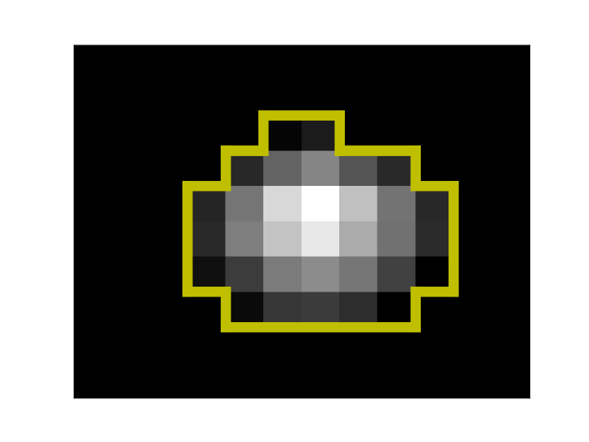
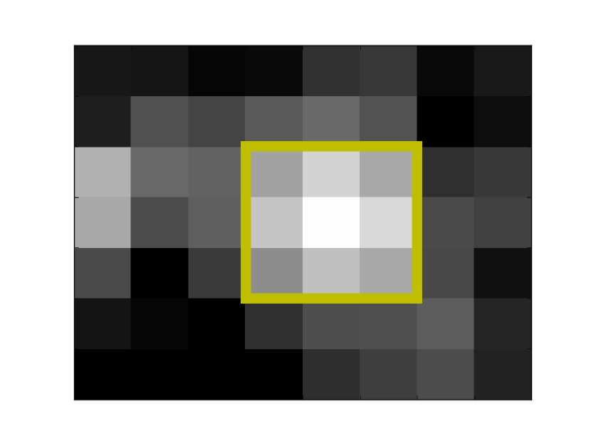
Figure 1: K2 stamps of K2-60 (left) and C7_8514 (right). The yellow lines represent the adopted photometric apertures. The pixel scale of the Kepler spacecraft is $3.98\arcsec$ per pixel. The stamp of K2-60 has a size of 12x10 pixels, whereas the stamp of C7_8514 has a size of 8x7 pixels. The gray scale represents the counts per pixel.

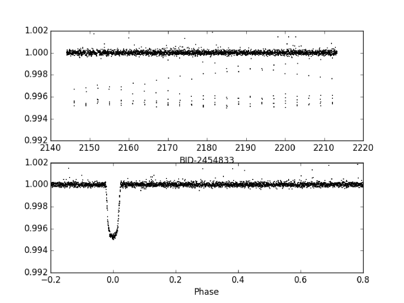
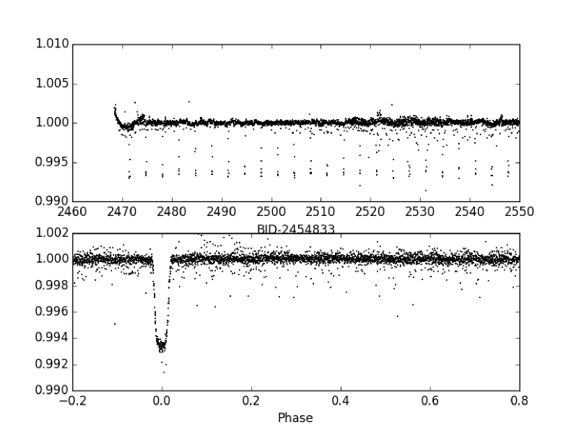
Figure 2: Corrected and normalized light curve of K2-60. The upper plot shows the normalized light curve over time. The lower plot displays the phase folded light curve.

Figure 3: Corrected and normalized light curve of C7_8514. Notation as in Figure 3.

2.2 High Dispersion Spectroscopy

We acquired five and eight high-resolution spectra ($R$ $\approx$ 67,000) of K2-60 and C7_8514 with the the FIbre-fed Échelle Spectrograph (FIES; Frandsen & Lindberg, 1999; Telting et al., 2014) between June and September 2016. FIES is mounted at the 2.56m Nordic Optical Telescope (NOT) of Roque de los Muchachos Observatory (La Palma, Spain). We adopted the same observing strategy as in Buchhave et al. (2010) and Gandolfi et al. (2015), i.e., we bracketed each science observation with long exposed ThAr spectra ($T_{\mathrm{exp}}$ $\approx$ 35 sec). The exposure time was set to 1800 – 3600 sec – according to sky conditions and scheduling constraints – leading to a signal-to-noise ratio (S/N) of 25–35 per pixel at 5500 Å. The FIES data were reduced using standard IRAF and IDL procedures. Radial velocity measurements were extracted via multi-order cross-correlation with the RV standard stars HD 50692 (catalog ) and HD 182572 (catalog ) (Udry et al., 1999) observed with the same instrument set-up as the target stars.

We also took three additional high-resolution spectra of K2-60 in July 2016 with the HARPS-N spectrograph (R $\approx$ 115,000; Cosentino et al., 2012) mounted at the 3.58m Telescopio Nazionale Galileo (TNG) at Roque de los Muchachos Observatory (La Palma, Spain). The exposure times were set to 1200 – 1500 seconds leading to a S/N of 15–20 per pixel at 5500 Å for the extracted spectra. We used the second fiber to monitor the Moon background and reduced the data with the HARPS-N dedicated pipeline. Radial velocities were extracted by cross-correlating the extracted spectra with a G2 numerical mask (Baranne et al., 1996; Pepe et al., 2002).

The FIES and HARPS-N RVs and their uncertainties are listed in Table 1, along with the bisector span (BIS) of the cross-correlation function (CCF). Time stamps are given in barycentric Julian day in barycentric dynamical time (BJD_TDB).

We searched for possible correlation between the RV and BIS measurements that might unveil activity-induced RV variations and/or the presence of blended eclipsing binary systems (Queloz et al., 2001). The Pearson correlation coefficient between the RV and BIS measurements of K2-60 is 0.11 with a p-value of 0.79. For C7_8514 the Pearson correlation coefficient is 0.10 with a p-value of 0.81. Adopting a threshold of 0.05 for the p-value confidence level (Lucy & Sweeney, 1971), the lack of significant correlations between the RV and BIS measurements of both stars further confirm that the observed Doppler variations are induced by the orbiting planets.

Table 1: FIES and HARPS-N RV measurements of K2-60 and C7_8514.

BJDTDB	RV	$\sigma_{\mathrm{RV}}$	BIS	Instr.
$-$2,450,000	(km s-1)	(km s-1)	(km s-1)
K2-60
7568.72048	$-$45.505	0.012	0.007	FIES
7569.72143	$-$45.394	0.024	$-$0.006	FIES
7570.71124	$-$45.490	0.012	0.022	FIES
7577.71171	$-$45.532	0.012	0.014	FIES
7578.64730	$-$45.422	0.030	0.018	FIES
7585.67140	$-$45.324	0.010	$-$0.036	HARPS-N
7586.68055	$-$45.362	0.006	$-$0.023	HARPS-N
7587.70160	$-$45.260	0.007	0.007	HARPS-N
C7_8514
7565.58753	$-$8.276	0.025	0.069	FIES
7566.56965	$-$8.404	0.023	0.012	FIES
7567.57489	$-$8.438	0.016	0.025	FIES
7568.59817	$-$8.272	0.021	0.044	FIES
7570.54490	$-$8.465	0.017	0.043	FIES
7628.44921	$-$8.273	0.029	$-$0.007	FIES
7637.39240	$-$8.392	0.016	0.004	FIES
7640.40979	$-$8.429	0.016	0.035	FIES

2.3 Imaging

Imaging with spatial resolution higher than that of K2 is used to detect potential nearby eclipsing binaries that could mimic planetary transit-like signals. It also enables us to measure the fraction of contaminating light arising from potential unresolved nearby sources whose light leaks into the photometric mask of K2, thus diluting the transit signal. Schmitt et al. (2016) observed K2-60 using the adaptive optics facility at the KECK telescope. They excluded faint contaminant stars as close as $0\farcs 25$ up to 4 magnitudes fainter than the target star.

We observed C7_8514 on 2016 September 13 (UT) with the ALFOSC camera mounted at the Nordic Optical Telescope. We used the Johnson’s standard R-band filter and acquired 16 images of 6 sec and 2 images of 20 sec. The data were bias subtracted and flat-fielded using dusk sky flats. The co-added 6-sec ALFOSC exposures are shown in Figure 4. We detected two nearby faint stars located $4.3\arcsec$ North-East and $6.0\arcsec$ South-East of C7_8514. They are 6.3 and 6.5 magnitudes fainter than the target and fall inside the photometric aperture that we used to extract the light curve of C7_8514 from the K2 images. We measured a contribution of $0.005\pm 0.001$ to the total flux, by contaminating sources for C7_8514. Our observations exclude additional contaminants out to a separation of $2\arcsec$ and up to 6 magnitudes fainter than the target. We compared our findings with the first data release from GAIA (Gaia Collaboration et al., 2016) and found a contamination factor of 0.0043, in agreement with our estimate. No additional sources are present in the GAIA catalog (Lindegren et al., 2016) within a radius of $10\arcsec$. The resolving power of GAIA is well below $1\arcsec$.

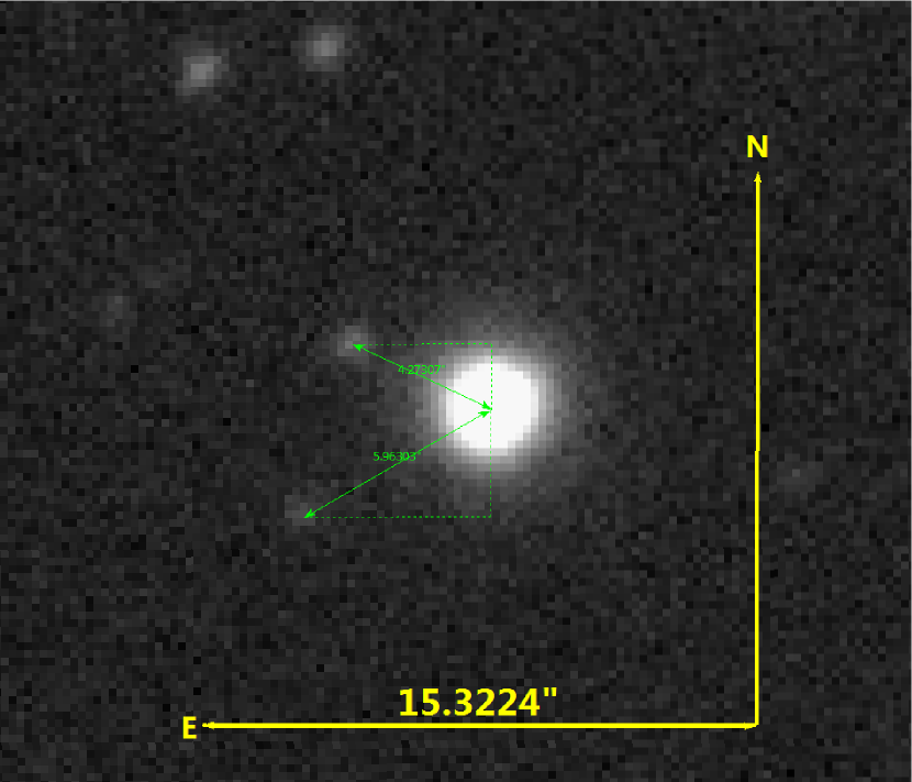
Figure 4: ALFOSC@NOT R-band image of C7_8514. We can resolve sources as close as $2\arcsec$ to our target star. C7_8514 and its two contaminants are marked with green circles.

3 Analysis

3.1 Spectral Analysis

We derived the spectroscopic parameters of K2-60 and C7_8514 from the co-added spectra used to extract the RVs of the stars (Sect. 2.2). The stacked FIES and HARPS-N have a S/N of 62 and 32 per pixel at 5500 Å; the co-added FIES data of C7_8514 have a S/N of 76 per pixel at 5500 Å. The analysis was carried out in three independent ways.

The first technique uses ATLAS 9 model spectra (Castelli & Kurucz, 2004) to fit spectral features that are sensitive to different photospheric parameters. We adopt the calibration equations of Bruntt et al. (2010) and Doyle et al. (2014) to determine the microturbulent ($V_{\mathrm{mic}}$) and macroturbulent ($V_{\mathrm{mac}}$) velocities. We mainly used the wings of the H_α and H_β lines to estimate the effective temperature ($T_{\mathrm{eff}}$), and the Mg i 5167, 5173, and 5184 Å, Ca i 6162 and 6439 Å, and the Na i D lines to determine the surface gravity log g_⋆. We simultaneously fit different spectral regions to measure the metal abundance [M/H]. The projected rotational velocity $v$ sin $i_{\star}$ was determined by fitting the profile of many isolated and unblended metal lines.

For the second method, micro-turbulent ($V_{\mathrm{mic}}$) and macroturbulent ($V_{\mathrm{mac}}$) velocities, as well as the projected stellar rotational velocity $v$ sin $i_{\star}$ were determined as described above. For the spectral analysis the second method relies on the use of the package SME (Spectroscopy Made Easy, where we used version 4.43) (Valenti & Piskunov, 1996; Valenti & Fischer, 2005). SME calculates, using a grid of models (we used the Atlas 12) for a set of given stellar parameters, synthetic spectra of stars and fits them to the observed high-resolution spectra using a $\chi$-square minimizing procedure.

The third method uses the equivalent width (EW) method to derive stellar atmospheric parameters: i ) $T_{\rm{eff}}$ is measured by eliminating trends between abundance of the chemical elements and the respective excitation potentials; ii ) log g_⋆ is derived by assuming the ionization equilibrium condition, i.e. requiring that for a given species, the same abundance (within the uncertainties) is obtained from lines of two ionization states (typically, neutral and singly ionized lines); iii ) microturbulent velocity is set by minimizing the slope of the relationship between abundance and the logarithm of the reduced EWs. We measured the equivalent widths using the DOOp program Cantat2014, a wrapper of DAOSPEC (Stetson & Pancino, 2008). We derived the photospheric parameters with the program FAMA (Magrini et al., 2013), a wrapper of MOOG (Sneden et al., 2012). The adopted atomic parameters are the public version of those prepared for the Gaia-ESO Survey (Heiter et al., 2015) and based on the VALD3 data (Ryabchikova et al., 2011). We typically used 200 Fe i lines and 10 Fe ii lines for the determination of stellar parameters.

The three methods provide consistent results within two sigma (see Table 2). The final adopted values are the weighted mean of the three independent determinations, using the error bars to calculate the weighting factor. The stellar parameters for both systems are listed in Table 3, along with the main identifiers and optical and near-infrared magnitudes.

Table 2: Effective temperature, surface gravity, and metallicity from different spectral analysis methods.

		K2-60			C7_8514
Method	$T_{\rm{eff}}$ (K)	log g⋆ (cgs)	[Fe/H] (dex)	$T_{\rm{eff}}$ (K)	log g⋆ (cgs)	[Fe/H] (dex)
Method 1	$5480\pm 85$	$4.05\pm 0.15$	$-0.10\pm 0.10$	$6050\pm 110$	$3.95\pm 0.10$	$0.08\pm 0.06$
Method 2	$5350\pm 90$	$3.95\pm 0.10$	$-0.10\pm 0.08$	$5970\pm 100$	$4.30\pm 0.15$	$0.08\pm 0.08$
Method 3	$5625\pm 115$	$4.22\pm 0.07$	$0.24\pm 0.15$	$6080\pm 150$	$3.95\pm 0.05$	$0.13\pm 0.16$

Table 3: Main identifiers, coordinates, magnitudes, and spectroscopic parameters of both systems.

Parameter	K2-60	C7_8514	Unit
RA	22h34m25s.49	18h59m56s.49	h
DEC	-13$\arcdeg$43′54′′.13	-22$\arcdeg$17′36′′.25	deg
2MASS ID	22342548-1343541	18595649-2217363	…
EPIC ID	206038483	216468514	…
Effective Temperature $T_{\rm{eff}}$	$5500\pm 100$	$6030\pm 120$	K
Surface Gravity log g⋆	$4.07\pm 0.11$	$4.07\pm 0.10$	cgs
Metallicity [Fe/H]	$0.01\pm 0.11$	$0.10\pm 0.10$	dex
$v$ sin $i_{\star}$	$2.2\pm 0.5$	$4.6\pm 0.5$	km s-1
Spectral Type	G4 V	F9 IV	…
B mag (UCAC4)	$13.56\pm 0.01$	$13.64\pm 0.01$	mag
V mag (UCAC4)	$12.79\pm 0.02$	$12.92\pm 0.01$	mag
J mag (2MASS)	$11.41\pm 0.02$	$11.56\pm 0.02$	mag
H mag (2MASS)	$11.09\pm 0.03$	$11.26\pm 0.03$	mag
K mag (2MASS)	$10.99\pm 0.02$	$11.21\pm 0.02$	mag

3.2 Joint Analysis of Photometric and Radial Velocity Measurements

We used the Transit Light Curve Modelling (TLCM) code (Csizmadia et al. 2015; Csizmadia et al. in prep.) for the simultaneous analysis of the detrended light curves and radial velocity measurements. TLCM uses the Mandel & Agol (2002) model to fit planetary transit light curves. The RV measurements are modeled with a Keplerian orbit. The fit is optimized using first a genetic algorithm and then a simulated annealing chain.

The fitted parameters are the semi-major axis $a/R_{*}$ and planet radius $R_{\mathrm{p}}/R_{*}$, both scaled to the radius of the star, the orbital inclination $i$, the limb darkening coefficients $u_{+}=u_{1}+u_{2}$ and $u_{-}=u_{1}-u_{2}$, the radial velocity semi amplitude $K$ and the systemic $\gamma$-velocity. The period ($P_{\mathrm{orb}}$) and epoch of mid-transit ($T_{0}$) are allowed to vary slightly around the values determined already by the detection.

For C7_8514b the model did not converge to the global minimum when leaving all nine parameters completely free, instead it seemed to converge to a broader local minimum. We thus first modeled the light curve, keeping the epoch and period, as well as the limb darkening coefficients fixed using estimates from Claret & Bloemen (2011). This gave us first estimates on the inclination, planet radius ratio, and semi major axis. In a second step we fitted all nine free parameters as for K2-60b, but restricted the parameter space with the priors as given by our first fit. To verify our results, We also modeled the light curve with different fixed inclinations, leaving all other parameters free. This confirmed our result of an high impact parameter.

We also fit the data for non-circular orbits. The best fitting eccentricity for K2-60 is $0.09\pm 0.03$ with a p-value of 0.90; as for C7_8514, we obtained $0.06\pm 0.05$ with a p-value of 0.57. Both p-values are larger than the 0.05 level of significance suggested by Lucy & Sweeney (1971). We concluded that the RV measurements do not allow us to prefer the eccentric solutions over the circular ones and thus fixed the orbit eccentricities to zero. This assumption is reasonable given the fact that short period orbits are expected to have circularized. Using the equations from Leconte et al. (2010), we calculated the tidal time-scales for the eccentricity evolution of the two systems. Assuming a modified tidal quality factor of $Q^{\prime}_{\star}=10^{6.5}$ for the stars and $Q^{\prime}_{\mathrm{p}}=10^{5.5}$ for the planets (Jackson et al., 2008), the timescales are $\sim$400 and $\sim$25 Myr for K2-60 and C7_8514, respectively. These time scales are shorter than the estimated ages of the two host stars (Table 4).

We also fitted for radial velocity trends that might unveil the presence of additional orbiting companions in the systems. We obtained radial accelerations that are consistent with zero.

The best fitting transit model and circular RV curve of K2-60b are shown in Figures 6 and 6, along with the photometric and RV data. Results for C7_8514b are displayed in Figures 8 and 8. We checked our results by performing a joint fit to the photometric and RV data using the MCMC code pyaneti (Barragán et al., in prep.). Following the same method outlined in Barragán et al. (2016), we set uninformative uniform priors in a wide range for each parameter and explored the parameter space with 500 chains. The final parameter estimates are consistent within 1-$\sigma$ with those obtained using TLCM.

From the results of the spectral analysis and joint data modeling, we used Yonsei-Yale (Yi et al., 2001; Demarque et al., 2004) and Dartmouth (Dotter et al., 2008) isochrones to estimate masses, radii, and ages of K2-60 and C7_8514. We obtained results that are in agreement regardless of the adopted set of isochrones. For the final results we used the Yonsei-Yale isochrones (Yi et al., 2001; Demarque et al., 2004). From the fundamental parameters of the host stars we calculated radii and masses of the two transiting planets. The parameter estimates are listed in Table 4 for both systems.

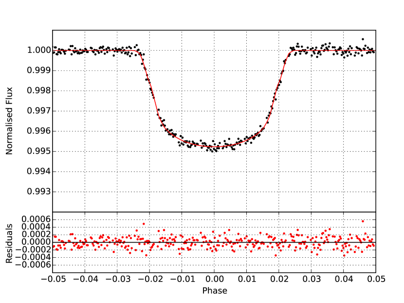
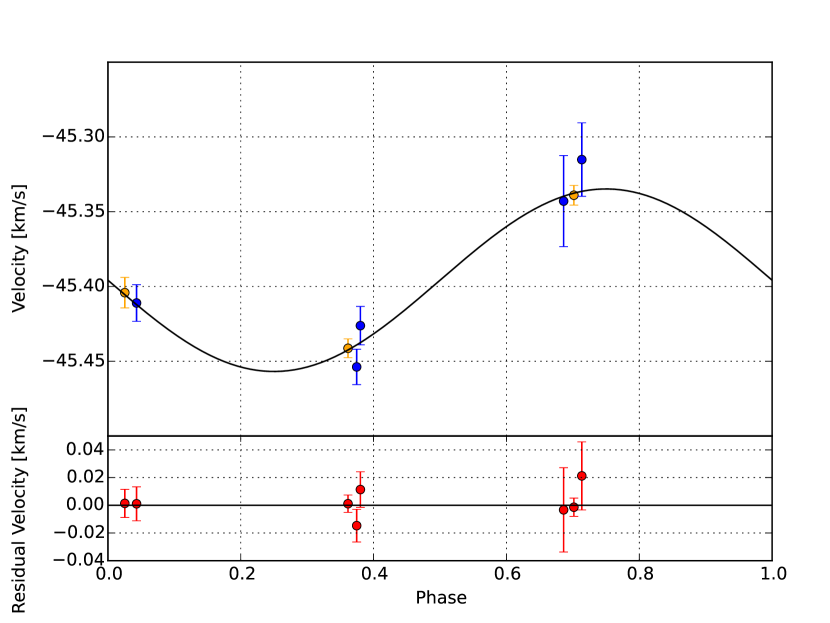
Figure 5: Phase folded light curve and best fitting transit model (red line) of K2-60b. Residuals to the fit are shown in the lower panel.

Figure 6: FIES (blue circles) and HARPS-N (orange circles) RV measurements of K2-60b and best fitting circular model. Residuals to the fit are shown in the lower panel.

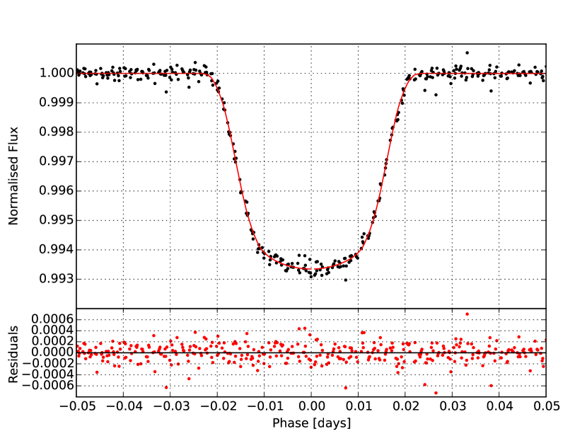
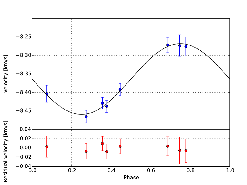
Figure 7: Phase folded light curve and the best fitting transit model (red line) of C7_8514b. Residuals to the fit are shown in the lower panel.

Figure 8: FIES RV measurements of C7_8514b and best fitting circular model. Residuals to the fit are shown in the lower panel.

4 Discussion and Summary

4.1 K2-60b

K2-60b is a transiting sub-Jovian planet with an orbital period of $3.00267\pm 0.00006$  days. It orbits a G4 main sequence star. The planet’s calculated effective temperature is $1400\pm 50$ K. With a radius of $0.683\pm 0.037$ $R_{\mathrm{Jup}}$ and a mass of $0.426\pm 0.037$ $M_{\mathrm{Jup}}$, it is more dense than expected. The radius anomaly, based on the difference between model estimated to observed radius as described in Laughlin et al. (2011), is $-0.46$, making this planet more dense than expected. Adaptive optics imaging by Schmitt et al. (2016) shows that there is no light contamination that could cause an underestimation of the planetary radius. We can exclude ellipsoidal variation with amplitudes above 0.05 mmag in the light curve. There is no obvious trend in the radial velocity data, although we can not exclude radial accelerations lower than 0.002 km s^-1day^-1.

The short orbital period and high effective temperature of the planet, along with its sub-Jovian size, put K2-60b close to the the so called sub-Jovian desert. Fig. 9 shows the known transiting planets with their radii plotted against their calculated effective temperatures as given by the equation in Laughlin et al. (2011)

$$T_{eff}=\left(\frac{R_{S}}{2a}\right)^{1/2}\frac{T_{S}}{(1-e^{2})^{1/8}}.$$ (1)

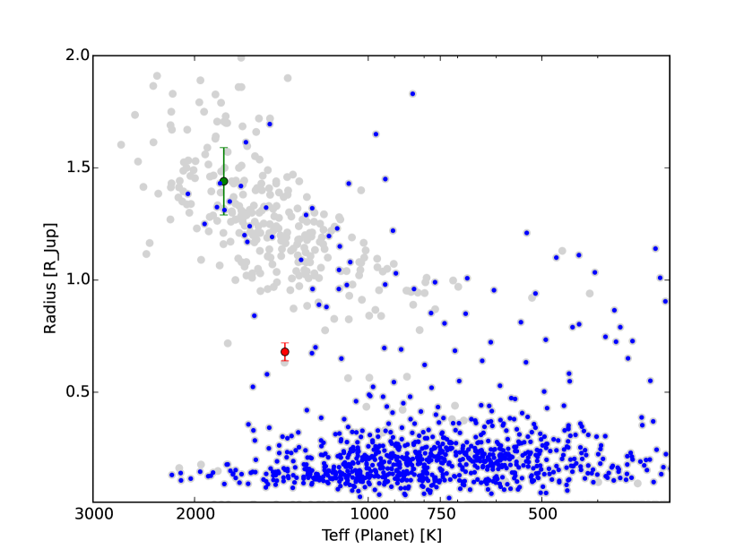
Figure 9: Planet radius over its orbit-averaged effective temperature. The gray dots show all planets. The blue dots mark planets that have been detected by the Kepler spacecraft (Kepler mission or K2 mission). The red dot denotes K2-60b and the green dot C7_8514b. The exoplanet data are taken from Extrasolar Planets Encyclopaedia (www.exoplanets.eu).

There is a clear lack of hot sub-Jovian planets. Due to different observational biases of exoplanet surveys (e.g., most of the inflated hot Jupiters have been detected by ground based surveys, which might not be able to detect sub-Jovian planets with the same efficiency) the upper border is not as well defined as it may seem. This can be seen by looking only at confirmed planets of the Kepler spacecraft (blue points in Fig. 9). Nevertheless, all observations suggest that the sub-Jovian desert exists, although its borders are not well defined. Only a few planets are known in this regime (e.g. Sato et al., 2005; Bonomo et al., 2014). K2-60b might help in the future to get better restrictions on its borders.

4.2 C7_8514b

C7_8514b is a Jovian planet on a short orbital period of $3.31392\pm 0.00002$ days. The planet orbits a F9 star about to leave the main sequence. It is one of only a few transiting planets known to orbit sub giants (e.g. Smith et al., 2016; Pepper et al., 2016; Van Eylen et al., 2016; Almenara et al., 2015). The planet’s calculated effective temperature is $1780\pm 90$ K its radius is $1.44\pm 0.15$ $R_{\mathrm{Jup}}$ and its mass is $0.84\pm 0.08$ $M_{\mathrm{Jup}}$. The radius anomaly is $+0.21$, making C7_8514b in contrast to K2-60b an highly inflated gaseous planet. Such high inflation has already been observed for other giant planets with a similar effective temperature (see Figure 9). As suggested by Laughlin et al. (2011), Ohmic heating might be at least partly responsible for such inflation of the planet.

Since it is projected against the galactic center, C7_8514 is in a relatively crowded stellar region. Using seeing-limited imaging and the GAIA public archive (DR1) we identify two faint stars within $\sim$$10\arcsec$. The resulting contamination factor of 0.005 has been taken into account when modeling the light curve. The radial velocity data do not show any significant eccentricity or long term trend higher than 0.001 km s^-1day^-1. The light curve of C7_8514 shows no ellipsoidal variation with an amplitude larger than 0.1 mmag.

Table 4: Parameters from light curve and RV data analysis.

Parameter	K2-60	C7_8514	Unit
Orbital period $P_{\mathrm{orb}}$	$3.00265\pm 0.00004$	$3.31392\pm 0.00002$	days
Transit epoch $T_{0}$	$6928.0593\pm 0.0007$	$7304.5244\pm 0.0002$	BJD${}_{\mathrm{TDB}}-2450000$
Transit Duration	$3.08\pm 0.10$	$3.19\pm 0.45$	hours
Scaled semi-major axis $a/R_{*}$	$7.78\pm 0.17$	$5.75\pm 0.31$
Semi-major axis $a$	$0.045\pm 0.003$	$0.048\pm 0.005$	au
Scaled planet radius $R_{P}/R_{*}$	$0.063\pm 0.001$	$0.083\pm 0.001$
Orbital inclination angle $i$	$88.49\pm 0.96$	$81.9\pm 0.7$	$\deg$
Impact parameter $b$	$0.21\pm 0.13$	$0.81\pm 0.08$
Limb-darkening coefficient $u_{+}$	$0.63\pm 0.08$	$0.51\pm 0.08$
Limb-darkening coefficient $u_{-}$	$0.29\pm 0.10$	$0.17\pm 0.07$
Radial velocity semi amplitude $K$	$61.0\pm 2.6$	$95.5\pm 1.3$	m s-1
Systemic radial velocity $\gamma$	$-45.475\pm 0.003$	$-8.364\pm 0.001$	km s-1
RV velocity offset between FIES and HARPS	$0.158\pm 0.004$	-	km s-1
Eccentricity $e$	0 (fixed)	0 (fixed)
Stellar mass $M_{*}$	$0.97\pm 0.07$	$1.30\pm 0.14$	$M_{\odot}$
Stellar radius $R_{*}$	$1.12\pm 0.05$	$1.78\pm 0.16$	$R_{\odot}$
$M^{1/3}_{*}/R_{*}$	$0.89\pm 0.02$	$0.61\pm 0.03$	Solar units
Stellar mean density $\rho_{*}$	$0.99\pm 0.06$	$0.33\pm 0.05$	g cm-3
Stellar surface gravity log g⋆	$4.33\pm 0.04$	$4.05\pm 0.07$	cgs
Age	$10.0\pm 3.0$	$4.25\pm 1.75$	Gyr
Planetary mass $M_{P}$	$0.426\pm 0.037$	$0.84\pm 0.08$	$M_{\mathrm{Jup}}$
Planetary radius $R_{P}$	$0.683\pm 0.037$	$1.44\pm 0.15$	$R_{\mathrm{Jup}}$
Planetary mean density	$1.7\pm 0.3$	$0.35\pm 0.1$	cgs
Planetary surface gravity log gp	$3.35\pm 0.06$	$3.00\pm 0.07$	cgs
Planetary calculated effective temperature	$1400\pm 50$	$1780\pm 90$	K

References

- Aigrain et al. (2015) Aigrain, S., Hodgkin, S. T., Irwin, M. J., Lewis, J. R., & Roberts, S. J. 2015, MNRAS, 447, 2880
- Alibert et al. (2011) Alibert, Y., Mordasini, C., & Benz, W. 2011, A&A, 526, A63
- Almenara et al. (2015) Almenara, J. M., Damiani, C., Bouchy, F., et al. 2015, A&A, 575, A71
- Barragán et al. (2016) Barragán, O., Grziwa, S., Gandolfi, D., et al. 2016, arXiv:1608.01165
- Barragán et al. (in prep.) Barragán, O., et al.
- Baranne et al. (1996) Baranne, A., Queloz, D., Ma/yor, M., et al. 1996, A&AS, 119, 373
- Batygin et al. (2016) Batygin, K., Bodenheimer, P. H., & Laughlin, G. P. 2016, ApJ, 829, 114
- Beaugé & Nesvorný (2013) Beaugé, C., & Nesvorný, D. 2013, ApJ, 763, 12
- Bodenheimer et al. (2003) Bodenheimer, P., Laughlin, G., & Lin, D. N. C. 2003, ApJ, 592, 555
- Bonomo et al. (2014) Bonomo, A. S., Sozzetti, A., Lovis, C., et al. 2014, A&A, 572, A2
- Borucki et al. (2010) Borucki, W. J., Koch, D., Basri, G., et al. 2010, Science, 327, 977
- Bruntt et al. (2010) Bruntt, H., Bedding, T. R., Quirion, P.-O., et al. 2010, MNRAS, 405, 1907
- Buchhave et al. (2010) Buchhave, L. A., Bakos, G. A., Hartman, J. D., et al. 2010, ApJ, 720, 1118
- Cabrera et al. (2012) Cabrera, J., Csizmadia, Sz., Erikson, A., Rauer, H., & Kirste, S. 2012, A&A, 548, A44
- Cantat-Gaudin et al. (2014) Cantat-Gaudin, T., Donati, P., Pancino, E., et al. 2014, A&A, 562, A10
- Carter & Winn (2010) Carter, J. A., & Winn, J. N. 2010, ApJ, 709, 1219
- Castelli & Kurucz (2004) Castelli, F., & Kurucz, R. L. 2004, arXiv:astro-ph/0405087
- Claret & Bloemen (2011) Claret, A., & Bloemen, S. 2011, A&A, 529, A75
- Cosentino et al. (2012) Cosentino, R., Lovis, C., Pepe, F., et al. 2012, in Society of Photo-Optical Instrumentation Engineers (SPIE) Conference Series, Vol. 8446, Society of Photo-Optical Instrumentation Engineers (SPIE) Conference Series, 1
- Crossfield et al. (2016) Crossfield, I. J. M., Ciardi, D. R., Petigura, E. A., et al. 2016, ApJS, 226, 7
- Csizmadia et al. (2015) Csizmadia, Sz., Hatzes, A., Gandolfi, D. et al. 2015, A&A, 584, A13
- Demarque et al. (2004) Demarque, P., Woo, J.-H., Kim, Y.-C., & Yi, S. K. 2004, ApJS, 155, 667
- Dotter et al. (2008) Dotter, A., Chaboyer, B., Jevremović, D., et al. 2008, ApJS, 178, 89-101
- Doyle et al. (2014) Doyle, A. P., Davies, G. R., Smalley, B., Chaplin, W. J., & Elsworth, Y. 2014, MNRAS, 444, 3592
- Frandsen & Lindberg (1999) Frandsen, S. & Lindberg, B. 1999, in “Astrophysics with the NOT”, proceedings Eds: Karttunen, H. & Piirola, V., anot. conf, 71
- Grziwa et al. (2012) Grziwa, S., Pätzold, M., & Carone, L. 2012, MNRAS, 420, 1045
- Grziwa et al. (2016a) Grziwa, S., Gandolfi, D., Csizmadia, Sz., et al. 2016a, AJ, 152, 132
- Grziwa et al. (2016b) Grziwa, S. & Pätzold, M. 2016b, arXiv:1607.08417
- Gaia Collaboration et al. (2016) Gaia Collaboration, Brown, A. G. A., Vallenari, A., et al. 2016, A&A, in press (arXiv:1609.04172)
- Gandolfi et al. (2015) Gandolfi, D., Parviainen, H., Deeg, H. J. et al., 2015, A&A, 576, A11
- Howell et al. (2014) Howell, S. B., Sobeck, C., Haas, M. et al., 2014, PASP, 126, 398
- Heiter et al. (2015) Heiter, U., Lind, K., Asplund, M., et al. 2015, Phys. Scr, 90, 054010
- Jackson et al. (2008) Jackson, B., Greenberg, R., & Barnes, R. 2008, ApJ, 678, 1396-1406
- Johnson et al. (2016) Johnson, M. C., Gandolfi, D., Fridlund, M., et al. 2016, AJ, 151, 171
- Laughlin et al. (2011) Laughlin, G., Crismani, M., & Adams, F. C. 2011, ApJ, 729, L7
- Leconte et al. (2010) Leconte, J., Chabrier, G., Baraffe, I., & Levrard, B. 2010, A&A, 516, A64
- Lindegren et al. (2016) Lindegren, L., Lammers, U., Bastian, U., et al. 2016, arXiv:1609.04303
- Lucy & Sweeney (1971) Lucy L. B., Sweeney M. A., 1971, AJ, 76, 544
- Lundkvist et al. (2016) Lundkvist, M. S., Kjeldsen, H., Albrecht, S., et al. 2016, Nature Communications, 7, 11201
- Magrini et al. (2013) Magrini, L., Randich, S., Friel, E., et al. 2013, A&A, 558, A38
- Mandel & Agol (2002) Mandel, K., and Agol, E. 2002, ApJ, 580, L171
- Matsakos & Königl (2016) Matsakos, T., & Königl, A. 2016, ApJ, 820, L8
- Mazeh et al. (2016) Mazeh, T., Holczer, T., & Faigler, S. 2016, A&A, 589, A75
- Mordasini et al. (2009a) Mordasini, C., Alibert, Y., & Benz, W. 2009a, A&A, 501, 1139
- Mordasini et al. (2009b) Mordasini, C., Alibert, Y., Benz, W., & Naef, D. 2009b, A&A, 501, 1161
- Mordasini et al. (2012) Mordasini, C., Alibert, Y., Benz, W., Klahr, H., & Henning, T. 2012, A&A, 541, A97
- Pepe et al. (2002) Pepe, F., Mayor, M., Galland, F. et al. 2002, A&A, 388, 632
- Pepper et al. (2016) Pepper, J., Rodriguez, J. E., Collins, K. A., et al. 2016, arXiv:1607.01755
- Queloz et al. (2001) Queloz, D., Henry, G. W., Sivan, J. P. et al. 2001, A&A, 379, 279
- Ryabchikova et al. (2011) Ryabchikova, T. A., Pakhomov, Y. V., & Piskunov, N. E. 2011, Kazan Izdatel Kazanskogo Universiteta, 153, 61
- Ryabchikova et al. (2015) Ryabchikova, T., Piskunov, N., Kurucz, R. L., et al. 2015, Phys. Scr, 90, 054005
- Telting et al. (2014) Telting, J. H., Avila, G., Buchhave, L., et al. 2014, AN, 335, 41
- Sato et al. (2005) Sato, B., Fischer, D. A., Henry, G. W., et al. 2005, ApJ, 633, 465
- Smith et al. (2016) Smith, A. M. S., Gandolfi, D., Barragán, O., et al. 2016, arXiv:1609.00239
- Southworth et al. (2007) Southworth, J., Wheatley, P. J., & Sams, G. 2007, MNRAS, 379, L11
- Schmitt et al. (2016) Schmitt, J. R., Tokovinin, A., Wang, J., et al. 2016, AJ, 151, 159
- Schneider et al. (2011) Schneider, J., Dedieu, C., Le Sidaner, P., Savalle, R., & Zolotukhin, I. 2011, A&A, 532, A79
- Sneden et al. (2012) Sneden, C., Bean, J., Ivans, I., Lucatello, S., & Sobeck, J. 2012, Astrophysics Source Code Library, ascl:1202.009
- Stetson & Pancino (2008) Stetson, P. B., & Pancino, E. 2008, PASP, 120, 1332
- Szabó & Kiss (2011) Szabó, G. M., & Kiss, L. L. 2011, ApJ, 727, L44
- Udry et al. (1999) Udry S., Mayor M., Queloz D., 1999, ASPC, 185, 367
- Valenti & Piskunov (1996) Valenti, J. A., & Piskunov, N. 1996, A&AS, 118, 595
- Valenti & Fischer (2005) Valenti, J. A., & Fischer, D. A. 2005, ApJS, 159, 141
- Van Eylen et al. (2016) Van Eylen, V., Albrecht, S., Gandolfi, D., et al. 2016, arXiv:1605.09180
- Vanderburg & Johnson (2014) Vanderburg, A., & Johnson, J. A. 2014, PASP, 126, 948
- Yi et al. (2001) Yi, S., Demarque, P., Kim, Y.-C., et al. 2001, ApJS, 136, 417