A model for structured information representation in neural networks

Abstract

Humans possess the capability to reason at an abstract level and to structure information into abstract categories, but the underlying neural processes have remained unknown. Experimental evidence has recently emerged for the organization of an important aspect of abstract reasoning: for assigning words to semantic roles in a sentence, such as agent (or subject) and patient (or object). Using minimal assumptions, we show how such a binding of words to semantic roles emerges in a generic spiking neural network through Hebbian plasticity. The resulting model is consistent with the experimental data and enables new computational functionalities such as structured information retrieval, copying data, and comparisons. It thus provides a basis for the implementation of more demanding cognitive computations by networks of spiking neurons.

Keywords: assemblies, Hebbian plasticity, binding, spiking neural networks, cognition

Running title: Structured representations in neural networks

1 Introduction

Consider the two sentences “The truck hit the ball” and “The ball hit the truck”. Even though they both consist of the same set of words, they convey fundamentally different information which is easily distinguished by a human listener. In order to do so, sentence information is represented in a structured manner in cortex that takes semantic roles of words (e.g., agent or patient) into account [FranklandGreene:15].

We can describe this problem on three different levels, corresponding to Marr’s levels of analysis [marr1982vision]. The computational level describes the high-level computational goal, which is the generation of a structured sentence representation. On the second, algorithmic level, we ask how structured representations can be implemented algorithmically. Recent experimental evidence (see below) suggests that on this algorithmic level, one predefined variable exist for each semantic role (we term them semantic variables). During language processing, contents (words) are assigned to these variables accordingly, an operation that is referred to as binding [plate1995holographic, van2006neural, eliasmith2012large, ajjanagadde1989efficient, shastri1999advances, hayworth2012dynamically, kriete2013indirection, zylberberg2013neuronal, hayworth2018thalamic, FriedericiSinger:15]. Finally, on the implementation level, these operations are implemented by the neuronal networks of the brain. In this work, we establish a connection between the latter two levels by showing how structured representations can emerge in a spiking neural network based on well-known neurophysiological mechanisms, and with minimal further assumptions.

A number of recent experimental findings shed some light onto the question of stimulus representations in the medial temporal lobe (MTL). It has been shown that “concept cells” located in the MTL underlie the representation of stimulus identity [quiroga2016neuronal]. Each concept cell responds to some unique concept present in the stimulus regardless of the mode of presentation, thus giving rise to a sparse representation of inputs. It has furthermore been shown that assemblies of concept cells in the MTL are not static, but can rapidly form new associations [IsonETAL:15].

In another key experiment, Frankland and Greene [FranklandGreene:15] investigated the cortical response to simple sentences like those discussed above using functional magnetic resonance imaging (fMRI; see also [wang2016identifying]). They showed that for some semantic variables (such as the agent or patient in a sentence), there exist specific subareas of the left mid-superior temporal cortex (lmSTC) which encode these variables. Importantly, after presenting some sentence, the content of these variables could be read out from the corresponding subareas, indicating that these variable-specific areas form content specific representations in the binding process. This finding, which cannot be reproduced by most existing binding models (see Discussion) forms the basis for the model presented in this article.

In the general form of binding, one or multiple features are bound to an object; this problem has been addressed by a host of models (see e.g., [plate1995holographic, van2006neural, eliasmith2012large, FriedericiSinger:15, von1994correlation]). In the specific variant of the binding problem considered here, a semantic variable is bound to a word in a sentence (one could describe this more generally as an abstract category being bound to some content, but we stay in the following in the realm of language processing). Models for binding typically rely on specifically constructed circuitry or specific connectivity between individual neurons or groups of neurons. It is unclear whether such detailed assumptions can be justified using the available data on cortical connectivity. A further open question is whether the specific wiring inherent to these models can emerge through plasticity mechanisms known to shape cortical networks.

To model the emergence of structured representations in view of the above experimental findings, we take a different approach: using minimal assumptions, we study a generic spiking neural network model solely using mechanisms supported by a large number of experimental data. In particular, we make no assumptions on specific wiring or symmetric connectivity. We model each variable-encoding subarea of the lmSTC – as identified by Frankland and Greene [FranklandGreene:15] – as one population of neurons with divisive inhibition [carandini2012normalization, wilson2012division, legenstein2017probabilistic, jonke2017feedback]. The full model may have several such “variable spaces”, one for each represented semantic variable. These variable spaces are sparsely connected to a single content space, where neuronal assemblies represent content which could be a word or a value. Hence, neurons in the content space model concept cells in the MTL [quiroga2016neuronal]. We propose that the control over binding processes between these spaces is implemented through disinhibition [Pfeffer:14, HarrisShepherd:15, LetzkusETAL:15, Caroni:15, FuETAL:15, FroemkeSchreiner:15]. When a variable space is disinhibited while an assembly is active in content space, a sparse assembly also emerges there. Fast Hebbian plasticity ensures that this assembly is stabilized and synaptically linked to the content space assembly. In other words, the variable space now contains a projection of the content space assembly. We refer to such a projection of an assembly to a variable space as an assembly projection. We propose that information about this assembly is retained in the variable space through transiently increased neuronal excitabilities [LetzkusETAL:15].

We show that this model can represent simple sentences in a structured manner by binding content from the content space to semantic variables encoded by the variable spaces. The resulting activity of the network is consistent with the fMRI data from Frankland and Greene [FranklandGreene:15]. We further show that this model is capable of performing additional elementary processing operations proposed as atomic computational primitives in the brain by Marcus et al. [MarcusETAL:14]: copying the content of one variable to another, and comparing the contents of two variables. Our results indicate that the concept of neural spaces and assembly projections extends the computational capabilities of neural networks in the direction of cognitive computation, symbolic computation, and the representation and computational use of abstract knowledge.

The presented model combines and extends ideas of previously proposed pointer-based and anatomical binding models (e.g. [zylberberg2013neuronal, hayworth2018thalamic], see Discussion for a comparison to existing models). By combining these ideas, we show the following key advances: (1) we show that binding of semantic variables to content is possible without the need for specific circuitry and wiring patterns, rather, binding emerges in generic spiking networks under Hebbian plasticity even under sparse network connectivity, (2) the encoding of information in the network is consistent with recent findings in the MTL (assembly representations through concept cells [quiroga2016neuronal]), (3) the model is consistent with recent fMRI data on structured sentence encoding in lmSTC [FranklandGreene:15], (4) the same model is capable of performing additional elementary processing operations [MarcusETAL:14], and (5) we prove the operativeness of the assembly pointer principle in a detailed spiking neural network model based on experimentally well-supported mechanisms.

2 Results

2.1 Generic network model for assembly projections

Experimental data obtained by simultaneous recordings from large sets of neurons through multi-electrode arrays or Ca²⁺ imaging showed that neural activity patterns in cortex can be characterized in first approximation as spontaneous and stimulus-evoked switching between the activations of different (but somewhat overlapping) subsets of neurons (see e.g. [Buzsaki:10, BathellierETAL:12, LuczakMacLean:12]). These subsets of neurons are often referred to as neuronal assemblies. Consistent with this experimental data, information about specific words/concepts and variables is represented in our model by corresponding assemblies of neurons in generic neural circuits, referred to as neural spaces in the following. In particular, we assume that specific content – which could be words, concepts, values, etc. – are encoded by assemblies in a neural space $\mathcal{C}$, which we refer to as the content space, see Fig. 1A.

Frankland and Greene showed that for some semantic variables (such the agent or patient in a sentence), there exist specific subareas of the lmSTC which encode these variables [FranklandGreene:15]. We model such subareas for variables $u,v,\dots$ as a distinct set of neural spaces $\mathcal{U},\mathcal{V},\dots$ and refer to these spaces as variable spaces in the following. Each variable space can be viewed as functioning like a register in a computer [FranklandGreene:15]. But in contrast to such registers, variable spaces do not store content directly. Instead, we hypothesize that a storage operation leads to the emergence of an assembly in the variable space, in particular an assembly which is linked via strong synapses to the assembly representing the particular content in the content space. We call these projections of assemblies to variable spaces assembly projections. In other words, by assembly projection we mean the emergence of an assembly in a variable space as the result of afferent activity by an assembly in the content space, with the establishment of strong synaptic links from the content assembly to the new one. From a computational viewpoint, such an assembly projection is a “pointer” (or “handle”) to a content in the content space.

Importantly, we do not assume specifically designed neural circuits which enable the creation of such assembly projections and thus variable binding. Instead, we assume a rather generic network for each variable space and the content space, with lateral excitatory connections and lateral inhibition within the space (a common cortical motif, investigated e.g. in [jonke2017feedback]). Furthermore, we assume that neurons in the content space are sparsely connected to neurons in variable spaces and vice versa, see Fig. 1A. We will show that the creation of an assembly projection in a variable space – implementing the binding of a variable to some content – emerges naturally in such generic circuits with random connectivity from plasticity processes.

In addition, our model takes into account that neurons typically do not fire just because they receive sufficiently strong excitatory input. Experimental data suggest that neurons are typically prevented from firing by an “inhibitory lock” which balances or even dominates excitatory input [HaiderETAL:13]. Thus, a generic pyramidal cell is likely to fire because two events take place: its inhibitory lock is temporarily lifted (“disinhibition”) and its excitatory input is sufficiently strong. A special type of inhibitory neuron (VIP cells) has been identified as a likely candidate for triggering disinhibition, since VIP cells target primarily other types of inhibitory neurons (PV+ and SOM+ positive cells) that inhibit pyramidal cells (see e.g. [HarrisShepherd:15]). Firing of VIP cells is apparently often caused by top-down inputs (VIP cells are especially frequent in layer 1, where top-down and lateral distal inputs arrive). Their activation is conjectured to enable neural firing and plasticity within specific patches of the brain through disinhibition (see e.g. [LetzkusETAL:15, Caroni:15, Pfeffer:14, FuETAL:15, FroemkeSchreiner:15]). One recent study also demonstrated that long-term plasticity in the human brain can be enhanced through disinhibition [CashETAL:16]. We propose that top-down disinhibitory control plays a central role for neural computation and learning in cortex by initiating for example the creation and reactivation of assembly projections. We note that we are not investigating the important question: which neural processes resulted in the decision to disinhibit this particular variable space – that is, to decide whether a word is the agent or patient of a sentence. We modeled disinhibition of neural spaces in the following way. As a default, excitatory neurons received an additional strong inhibitory current that silenced the neural space. The space was disinhibited by the removal of this inhibitory current, which enabled activity in the neural space if excitatory input was sufficiently strong (see Supplement S1).

2.2 Emergence of assembly projections through Hebbian plasticity

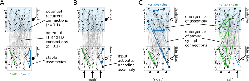
Figure 1: Neural spaces and assembly projections. A) Network structure. Rectangles indicate content space $\mathcal{C}$ (white, bottom) and variable space $\mathcal{V}$ for variable $v$ (light blue, top). Circles denote neurons (open: inactive; filled: active). Disinhibition is shown on the right of each space (filled black circle: inhibited; open circle: disinhibited). Concepts are encoded in the content space through stable assemblies (only two assemblies for two contents “ball” and “truck” are shown, strong recurrent connections are depicted with colors based on assembly identity). Thin gray lines between $\mathcal{C}$ and $\mathcal{V}$ as well as within $\mathcal{V}$ show potential feedforward, feedback, and recurrent connections (randomly initiated, $p=0.1$). Only a subset of 25 neurons is shown per space. B) Presentation of a concept (bottom, arrows) activates the encoding assembly in the content space if it is disinhibited (filled dots: active neurons). Initially, the variable space $\mathcal{V}$ is inhibited, preventing plasticity from occurring at the potential feedforward/feedback and recurrent connections. C) Disinhibition of the variable space enables the activation of neurons there and results in the formation of an assembly projection. Hebbian plasticity at the potential connections leads to the emergence of an assembly in the variable space (strong recurrent connections are shown in $\mathcal{V}$) which has strong synaptic connectivity with the active assembly in $\mathcal{C}$ (solid lines: feedforward connections, i.e. from $\mathcal{C}$ to $\mathcal{V}$; dashed: feedback). This mechanism allows the assignment of values to the variable encoded by the variable space. Assignment of different values (left: “truck”, right: “ball”) give rise to different assembly projections (i.e. different assemblies in $\mathcal{V}$ and different connectivity between $\mathcal{V}$ and $\mathcal{C}$, color encodes identity of the value assigned to the variable space).

To test whether the binding of content to variables can be performed by generic neural circuits, we performed computer simulations where stochastically spiking neurons were embedded in the following network structure (see Fig. 1A): The network consisted of a content space $\mathcal{C}$ with 1000 excitatory neurons and a single variable space $\mathcal{V}$ for a variable $v$ consisting of 2000 excitatory neurons. In both spaces, neurons were recurrently connected (connection probability $0.1$) and lateral inhibition was implemented by means of a distinct inhibitory population to ensure sparse activity. Connections between $\mathcal{C}$ and $\mathcal{V}$ were introduced randomly with a connection probability of $0.1$. Neurons in the content space additionally received connections from $200$ input neurons whose activity indicated the presence of a particular input stimulus. Hebbian-type plasticity is well-known to stabilize assemblies (see e.g. [litwin2014formation, pokorny2017associations]) and it can also strengthen connections bidirectionally between variable spaces and the content space. In our model, this plasticity has to be reasonably fast so that connections can be strengthened within relatively short stimulus presentations. As a Hebbian-type plasticity, we used in our spiking neural network model spike timing-dependent plasticity (STDP; [bi1998synaptic, caporale2008spike]) for all synapses between excitatory neurons in the circuit (see Supplement S1 for more details). Other synapses were not plastic.

Emergence of content assemblies

We do not model the initial processing of speech, which is in itself a complicated process. Instead, we assume that assemblies in content space act as tokens for frequently observed input patterns that have already been extracted from the sensory stimulus. Hence, we induced assemblies in content space $\mathcal{C}$ by an initial repeated presentation of simple rate patterns provided by $200$ spiking input neurons (see Supplement S2). We first defined five such patterns $P_{1},\dots,P_{5}$ that modeled the input to this space when a given content (e.g., the word “truck” or “ball”) is experienced. These patterns were repeatedly presented as input to the disinhibited content space (the value space remained inhibited during this presentation). Due to these pattern presentations, an assembly $\mathcal{C}(P_{i})$ emerged in content space for each of the patterns $P_{i}$ (assembly sizes typically between $50$ and $90$ neurons) that was robustly activated (average firing activity of assembly neurons $>50$ Hz) whenever the corresponding pattern was presented as input, see Fig. 1B. STDP of recurrent connections led to a strengthening of synapses within each assembly, while synapses between assemblies remained weak (see Supplement S2 for details).

Emergence of assembly projections

Assume that an active assembly $\mathcal{C}(P)$ in content space represents some content $P$ (such as the word “truck”). A central hypothesis of this article is that disinhibition of a variable space $\mathcal{V}$ leads to the creation of an assembly projection $\mathcal{V}(P)$ in $\mathcal{V}$. This projection $\mathcal{V}(P)$ is itself an assembly (like the assemblies in the content space) and interlinked with $\mathcal{C}(P)$ through strengthened synaptic connections.

To test this hypothesis, we next simulated disinhibition of the variable space $\mathcal{V}$ while input to content space $\mathcal{C}$ excited an assembly there. This disinhibition of the variable space allowed spiking activity of some of the neurons in it, especially those that received sufficiently strong excitatory input from a currently active assembly in the content space. STDP at the synapses that connected the content space $\mathcal{C}$ and the variable space $\mathcal{V}$ led to the stable emergence of an assembly $\mathcal{V}(P_{i})$ in the variable space within one second when some content $P_{i}$ was represented in $\mathcal{C}$ during disinhibition of $\mathcal{V}$, see Fig. 1C. Further, plasticity at recurrent synapses in the variable space $\mathcal{V}$ induced strengthening of recurrent connections within assemblies there (see Fig. 1C and Supplement S2). Hence, disinhibition led to the rapid and stable creation of an assembly in the variable space $\mathcal{V}$, i.e., an assembly projection. We denote such creation of an assembly projection in a variable space $\mathcal{V}$ for a specific variable $v$ to content $P$ encoded in content space by $\text{CREATE}(v,P)$.

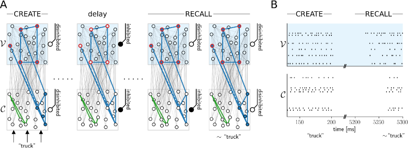
Figure 2: Variable-specific recall through assembly projections. A) Recall of a previously created assembly projection (schematic drawing). After an assembly projection was formed (CREATE) for the word “truck”, the excitability of assembly neurons in the variable space $\mathcal{V}$ is enhanced (indicated by red color). When the variable space is disinhibited, these neurons are activated, and in turn they activate the “truck” assembly in content space $\mathcal{C}$ (RECALL). B) Spike rasters from variable space $\mathcal{V}$ (top) and content space $\mathcal{C}$ (bottom) in a simulated recall (only $20$ randomly selected neurons shown per neural space for clarity). After a CREATE (left, up to $200$ ms), and a delay for $5$ s, a RECALL is initiated by first disinhibiting the variable space $\mathcal{V}$ (at time $t=5200$ ms) and then disinhibiting the content space $\mathcal{C}$ ($50$ ms later).

Fast recruitment of assemblies in a variable space necessitates rapid forms of plasticity. We assumed that a (possibly initially transient) plasticity of synapses occurs instantaneously, even within seconds. The assumption of rapid plasticity of neurons and/or synapses is usually not included in neural network models, but it is supported by a number of recent experimental data. In particular, [IsonETAL:15] shows that neurons in higher areas of the human brain change their response to visual stimuli after few or even a single presentation of a new stimulus where two familiar images are composed into a single visual scene.

Variable-specific recall through assembly projections

From a functional perspective, the binding of a content to a semantic variable is exploited at a later point in time when the content of this variable is recalled for further processing. In our model, a recall $\text{RECALL}(v)$ of the variable’s $v$ content should lead to the activation of the assembly $\mathcal{C}(P)$ in content space which was active at the most recent $\text{CREATE}(v,P)$ operation (e.g., representing the word “truck”). The strengthened synaptic connections between assemblies in variable space $\mathcal{V}$ for variable $v$ and content space $\mathcal{C}$ may in fact enable such a recall. However, an additional mechanism is necessary that reactivates the most recently active assembly in variable space $\mathcal{V}$. One possible candidate mechanism is the activity-dependent change of excitability in pyramidal cells. It has been shown that the excitability of pyramidal cells can be changed in a very fast but transient manner through fast depression of GABA-ergic synapses onto pyramidal cells [KullmannETAL:12]. This effect is potentially related to the match enhancement or match suppression effect observed in neural recordings from monkeys, and is commonly used in neural network models for delayed match-to-sample (DMS) tasks (see e.g. [TartagliaETAL:15]). Using such a mechanism, a $\text{RECALL}(v)$ can be initiated by disinhibition of the variable space $\mathcal{V}$ while the content space does not receive any bottom up input, see Fig. 2A. The increased excitability of recently activated neurons in $\mathcal{V}$ ensures that the most recently active assembly is activated which in turn activates the corresponding content through its (previously potentiated) feedback connections to content space $\mathcal{C}$.

We tested whether such a mechanism can reliably recall previously bound contents from variables in our generic network model. A transient increase in neuron excitability has been included in the stochastic spiking neuron model through an adaptive neuron-specific bias that increases slightly for each postsynaptic spike and decays with a time constant of $5$ seconds (see Supplement S2). We used an automated optimization procedure to search for synaptic plasticity parameters that lead to clean recalls (see Supplement S2, all parameters were constrained to lie in biologically realistic ranges). Fig. 2B shows the spiking activity in our spiking neural network model for an example recall $5$ seconds after the creation of the assembly projection. One sees that the assembly pattern that was active at the create operation was retrieved at the recall.

In general, we found that the contents of the projection can reliably be recalled in our model. In order to test whether the model can deal with the high variability of individual randomly created networks as well as with the variability in sizes and connectivity of assemblies, we performed several simulations with random network initializations. We used five different content space instances with randomly chosen recurrent connections. In each of those, we induced five stable assemblies encoding different contents as described above. Note that these assemblies emerged through a plasticity process, so their sizes were variable. For each of these five content space instances, we performed ten simulations where the variable space was set up and randomly connected in each of these. This procedure ensured that we did not test the network behavior on a particular instantiation of the circuit, but rather whether the principle works reliably for generic randomly connected circuits.

Performing a CREATE/RECALL sequence separately for each of the five patterns, we found that the recall was successful in each of the $250$ trials ($5$ content spaces with $5$ patterns each, and this repeated $10$ times for different variable spaces). A recall was regarded as a success if during the RECALL phase, at least $80$% of the neurons which previously belonged to the concept assembly (measured after the assembly induction in the content space) were active (firing rate $>50$ Hz), and if the number of erroneously active neurons did not exceed $20$% of the original assembly size. Typically, one or two neurons from the original assembly were missing, but no excess neurons fired during the RECALL.

2.3 Reproducing experimental data on the binding of words to roles and structured information representation

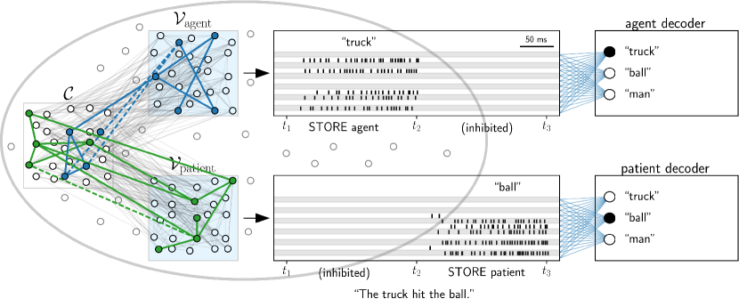
Figure 3: Decoding of agent/patient identity from assembly projection, as in [FranklandGreene:15]. The content space $\mathcal{C}$ (white background, left) was connected to two neural spaces for storing the agent (light blue background, top) and the patient (light blue background, bottom) of a sentence. Presentation of a word lead to the activation of the corresponding assembly in $\mathcal{C}$ (only the words for the agent and the patient were processed, verbs and articles were ignored). Words were presented in the order in which they appear in the sentence (for “The truck hit the ball.”, the input “truck” was presented while the agent space was disinhibited between $t_{1}$ and $t_{2}$, likewise disinhibition of the patient space while “ball” was presented between $t_{3}$ and $t_{4}$). This resulted in the establishment of assembly projections within the variable spaces for agent and patient (insets show spike rasters of a subset of neurons from each variable space). Linear classifiers (“agent decoder” and “patient decoder”) were able to determine the current agent and patient in sentences from the corresponding variable spaces, modeling experimental results in [FranklandGreene:15]. The information could be decoded from the variable space.

Two experiments performed in [FranklandGreene:15] provided new insights in how variables may be encoded in neocortex. Sentences were shown to participants where individual words (like “truck” or “ball”) occur as the agent or as the patient. The authors then studied how cortex represents the information contained in a sentence. In a first experiment, the authors aimed to identify cortical regions that encode sentence meaning. Example sentences with the words ”truck” and “ball” are “The truck hit the ball” and “The ball hit the truck”. The different semantics of these sentences can be distinguished for example by answering the question “What was the role of the truck?” (with the answer “agent” or “patient”). Indeed, the authors showed that a linear classifier is able to distinguish these sentences from the fMRI signal of left mid-superior temporal cortex (lmSTC). Using our model for assembly projections, we can model such situations by binding words either to an agent variable (“who did it”) or to a patient variable (“to whom it was done”). Under the assumption that lmSTC hosts variable spaces (with assembly projections) for the role of words, it is expected that semantic decoding is possible from the activity there, but not from the activity in content space where the identities are encoded independently of their role. We performed simulations where the words “truck” and “ball” (represented by some assemblies in content space) were sequentially bound (the temporal sequence was mimicking the position of the word in the sentence) either to variable space $\mathcal{V}_{\text{agent}}$ or $\mathcal{V}_{\text{patient}}$, depending on their role. Note that we did not model the processing of the verb or other words in the sentence, as only the representation of the agent and the patient was investigated in [FranklandGreene:15]. Low-pass filtered network activity was extracted for each of the resulting four sequences. We then trained a linear classifier to classify the role of “truck” for each time point during the sequential binding, based on a noisy version of filtered network activity. We found that even under severe noise conditions, the classifier was able to nearly perfectly classify test sentences (i.e., new simulations with new noisy activity on the same sentences; test classification error $3.0$ %). On the other hand, a classifier based on activity of the content space performed only slightly better than random with a test classification error of $44.4$ %.

A second experiment in [FranklandGreene:15] revealed that information from lmSTC subregions can also be used to read out the current contents of the variables for the agent and the patient. More specifically, the authors showed that it is possible to predict the identity of the agent from the fMRI signal of one subregion of lmSTC and the identity of the patient from the signal in another subregion (generalizing over all identities of other roles and over different verbs). We expected that this would also be the case in the proposed model since the assemblies that are formed in the variable spaces $\mathcal{V}_{\text{agent}}$ and $\mathcal{V}_{\text{patient}}$ are typically specific to the bound content. We tested this hypothesis by training a multinomial logistic regression model to classify the content of the variable for each of the two variable spaces (agent and patient) at times when these spaces were disinhibited (Fig. 3, “agent decoder” and “patient decoder”). Here, we bound words to variable spaces as before, but we considered all $40$ possibilities of how $5$ items (words) $A_{1},\dots,A_{5}$ can be sequentially bound (for example: $A_{1}$ is bound first to $\mathcal{V}_{\text{agent}}$ , then $A_{2}$ is bound to $\mathcal{V}_{\text{patient}}$ ; we excluded sentences where the agent and patient is the same word). Low-pass filtered activity of a subset of neurons was sampled at every $1$ ms to obtain the feature vectors to the classifiers (see Supplement S2). Half of the possible sequences were used for testing where we made sure that the two items used in a given test sentence have never been shown in any combination in one of the sentences used for training. Consistent with the results in [FranklandGreene:15], the classifier achieved nearly optimal classification performance on test data (classification error $<3$ % for each variable space). Note that such classification would fail if each variable space consisted of only a single assembly that is activated for all possible fillers [zylberberg2013neuronal], since in this case no information about the identity of the role is available in the variable space.

2.4 Cognitive computations with assembly projections

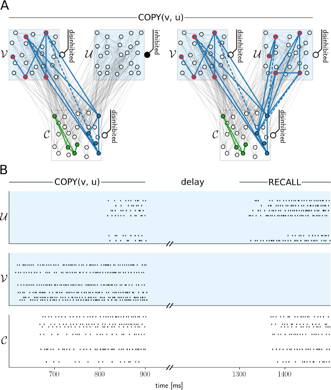
Figure 4: Assembly projection copy operation. A) Copying the content of one variable space to another variable space (schematic drawing). Disinhibition of variable space $\mathcal{V}$ recalls its content in content space $\mathcal{C}$ (left). A subsequent disinhibition of variable space $\mathcal{U}$ creates an assembly projection for this content there (right). B) Spike rasters from variable spaces $\mathcal{U}$ (top), $\mathcal{V}$ (middle), and content space $\mathcal{C}$ (bottom) in a simulated copy operation from a variable $v$ to a variable $u$ ($600-900$ ms; only $20$ randomly selected neurons are shown per neural space for clarity). After a $400$ ms delay, the content of variable $u$ is tested by a recall at time $1300$ ms. The assembly is correctly recalled into the content space.

Apart from the creation of assembly projections and recall of content, two further operations have been postulated by Marcus et al. to be essential for many higher cognitive functions [zylberberg2013neuronal]. The first is $\text{COPY}(v,u)$ which copies (or routes) the content of variable $v$ to variable $u$. In our model, the copy operation can be realized by creation of an assembly projection in variable space $\mathcal{U}$ for variable $u$ to the content to which the assembly projection in variable space $\mathcal{V}$ for variable $v$ refers to. We hypothesized that this operation can be implemented in our generic circuit model simply by disinhibiting $\mathcal{V}$ in order to activate the corresponding content in $\mathcal{C}$ followed by a disinhibition of $\mathcal{U}$ in order to create an assembly projection there, see Fig. 4A.

To test this hypothesis, we performed simulations of our spiking neural network model with one content space and two variable spaces. The performance was tested through a recall from the target assembly projection $400$ ms after the projection was copied, see Fig. 4B. We deployed the same setup as described above where $5$ assemblies were established in the content space, again considering ten different pre-trained content space instances (see above). For each of these, we performed ten copy operations (testing twice the copying of each content assembly) and assessed the assembly active in the content space after a recall from the target variable space. Again, all of the 100 considered cases were successful (applying the same success criterion as before).

A final fundamental operation considered in [zylberberg2013neuronal] is $\text{COMPARE}(v,u)$ which assesses whether the content of $v$ is equal to the content of $u$. One possible implementation of this operation in our model is established by a group of readout neurons which receive depressing synaptic connections from the content space. Then, when the content for $\mathcal{V}$ and $\mathcal{U}$ is recalled in sequence, the readout synapses will be depressed for the content of $\mathcal{U}$ if and only if the content of $\mathcal{U}$ equals the content of $\mathcal{V}$. Such a “change detecting” readout population thus exhibits high activity if the contents of $\mathcal{V}$ and $\mathcal{U}$ are different, see Fig. 5A. Simulation results from our spiking neural network model are shown in Fig. 5B, C. Using a set of $5$ contents as above, we tested $25$ comparisons in total, one for each possibility how these $5$ contents can be bound to two variable spaces for variables $v$ and $u$. Fig. 5B shows readout activity for the case when the same content was bound to both variables $v$ and $u$ (5 cases). The readout activity of the second recall (starting after time $200$ ms) was virtually absent in this case. In contrast, if the two variables were bound to different content (20 cases), the second recall always induced strong activity in the readout population (Fig. 5C). Hence, this simple mechanism is sufficient to compare variables with excellent precision by simply thresholding the activity of the readout population after the recall from the second assembly projection.

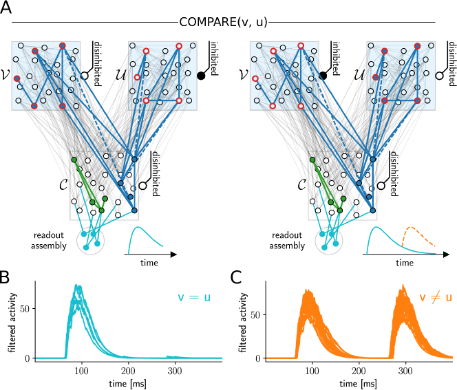
Figure 5: Comparison with assembly projections. A) Comparing the content of two variable spaces (schematic drawing). A population of readout neurons (bottom, teal) receives sparse depressing connections from the excitatory neurons in the content space. The comparison consists of a recall from variable space $\mathcal{V}$ (left; red neurons indicate neurons with higher excitability) followed by a recall from $\mathcal{U}$ (right). During the first recall, readout weights become depressed and readout activity decreases (indicated by teal trace inset right of readout). Next, a second recall is performed (right). If the patterns are identical, the readout weights are still depressed and the readout response is therefore weak (teal trace at readout). If the content changes (i.e., $u\neq v$), readout weight from active neurons in $\mathcal{C}$ are not depressed, which leads to strong readout activity (dashed orange trace at readout). B, C) Resulting readout assembly activity in spiking neural network model. Each trace shows the population activity (filtered with an exponential kernel) of the readout population for one comparison operation between two assembly projection contents ($25$ comparisons in total, one for each possible way of assigning $5$ values to two variable spaces for variables $v$ and $u$). At time $0$ ms, the content of variable space $\mathcal{V}$ was recalled (during the first $50$ ms of each recall, the content space remains inhibited and thus there is no readout activity) and the readout reacted in a similar manner to all contents. From time $200$ ms on, the content of variable space $\mathcal{U}$ was recalled. Due to depressed synaptic connections, the readout response was weak when the content of $\mathcal{V}$ matched the content of $\mathcal{U}$ (panel B). In case $\mathcal{V}$ and $\mathcal{U}$ stored different values the response was as strong as during the first recall phase (panel C).

3 Discussion

It has often been emphasized (see e.g. [Marcus:03, MarcusETAL:14]) that there is a need to understand brain mechanisms for information processing via variables. We show in this article how binding capabilities emerge in a generic network of spiking neurons by means of assembly projections. Our model is consistent with recent findings on cortical assemblies and the encoding of sentence meaning in cortex [FranklandGreene:15]. Our neural network model is not specifically constructed to perform such binding tasks. Instead, it is based on generic sparsely and randomly connected neural spaces that organize their computation based on fast plasticity mechanisms. The model provides a direct link between information processing on the algorithmic level of symbols and sentences and processes on the implementation level of neurons and synapses. The resulting model for brain computation supports top down structuring of incoming information, thereby laying the foundation of goal oriented “willful” information processing rather than just input-driven processing. The proposed synaptic plasticity that links assemblies in different neural spaces can be transient, but could also become more permanent if its relevance is underlined through repetition and consolidation. This would mean that some neurons in the variable space are no longer available to form new projection assemblies, but this does not pose a problem if each variable space is sufficiently large.

A large body of modeling studies have tackled the general binding problem. We study in this work not the standard form of a binding task, where for example one or several features are bound to an object (see, e.g. [plate1995holographic, van2006neural, eliasmith2012large, FriedericiSinger:15] for models in that direction). Instead, we are addressing the problem of binding abstract categories, i.e., structural information, to content. The main classes of models in this direction are pointer-based models and models based on indirect addressing. Pointer-based models (e.g. [zylberberg2013neuronal]) assume that pointers are implemented by single neurons or populations of neurons which are always co-active. In contrast, our model is based on the assumption that distributed assemblies of neurons are the fundamental tokens for encoding symbols and content in the brain, and also for projections which implement in our model some form of pointer. We propose that these assembly projections can be created on the fly in some variable spaces and occupy only a sparse subset of neurons in these spaces. [FranklandGreene:15] showed that the identity of a thematic role (e.g. the agent in a sentence) can be predicted from the fMRI signal of a subregion in temporal cortex when a person reads a sentence. As shown above, this finding is consistent with assembly projections. It is, however, inconsistent with models where a variable engages a population of neurons that is independent of the bound content, such as pointer-based models. In comparison to pointer models, the assembly projection model could also give rise to a number of functional advantages. In a variable space $\mathcal{V}$ for a variable $v$, several instantiations of the variable can coexist at the same time, since they can be represented there by increased excitabilities of different assemblies. These contents could be recalled as different possibilities in a structured recall and combined in content space $\mathcal{C}$ with the content of other variables to in order to answer more complex questions.

Models based on indirect addressing assume that a variable space encodes an address to another brain region where the corresponding content is represented [kriete2013indirection]. The data of Frankland and Greene, which shows that the stored content can be decoded from the brain area that represents its thematic role, speak against this model in its pure form, as the address is in general unrelated to the stored content.

Another category are anatomical binding models in which different brain areas are regarded as distinct placeholders (similar to the variable spaces in this work). As each placeholder may have a unique representation for some content, anatomical binding models are consistent with the findings of Frankland and Greene [FranklandGreene:15]. A problem in anatomical binding models lies in providing a mechanisms which allows to translate between the different representations. Building on previous work [hayworth2012dynamically], a recent non-spiking model shows how external circuitry can be used to solve this problem [hayworth2018thalamic]. Each pair of placeholders requires multiple external processing circuits which are densely connected to the placeholders to allow transferring and comparing contents. The number of these processing circuits increases quadratically with the number of placeholders. In contrast, the model presented in this work circumvents this problem by using the content space as a central hub, removing the need for additional circuitry.

In summary, the presented model combines the strengths of pointer-based (e.g. [zylberberg2013neuronal]) and anatomical binding models (e.g. [hayworth2018thalamic]). Like anatomical binding models [hayworth2018thalamic], the dynamics of the proposed model match experimental data on the encoding of variables in human cortex [FranklandGreene:15], but using the content space as a central hub eliminates the need to add circuitry as the number of variables increases. This is achieved by using a pointer-based mechanism, but unlike pointer models [kriete2013indirection, zylberberg2013neuronal] the proposed model is consistent with the findings of [FranklandGreene:15] and does not rely on elaborate processing circuitry or dense bidirectional connectivity.

The validity of the assembly projection model could be tested experimentally, since it predicts quite unique network dynamics during mental operations. First, binding of a variable to a concept employs disinhibition of a variable space related to that variable. This could be implemented by the activation of inhibitory VIP cells which primarily target inhibitory neurons, or by neuromodulatory input. Similar disinhibition mechanisms would be observed during a recall of the filler for that variable. Another prediction of the model is that the assembly projection that emerges in a variable space for some content should be similar to another one for the same content if it is re-established on a short or medium time scale. On the other hand, a significant modification of the assembly that encodes a concept will also modify the assembly projection that emerges in a variable space. Further, our model suggests that inactivation of an assembly projection to some content $A$ in variable space $\mathcal{V}$ would not abolish the capability to create a binding of the associated variable $v$ to this content $A$: If the trial that usually creates this binding is repeated, a new assembly projection in the variable space for $v$ can emerge. Finally, the model predicts that a mental task that requires to copy (or compare) the filler of one variable $u$ to another variable $v$ causes sequential activation (disinhibition) of the variable spaces $\mathcal{U}$ and $\mathcal{V}$ for these variables.

The assembly projection model assumes that there is sufficient connectivity between the content space and variable spaces in both directions such that assemblies can be mutually excited. The most prominent language related areas in the human brain are Broca’s area and Wernicke’s area. In addition, it has been speculated that word-like elements are stored in the middle temporal cortex [berwick2016only], corresponding to the content space in our model. As discussed in [berwick2016only], these areas are connected by strong fiber pathways in adult humans. These pathways could provide the necessary connectivity for the creation of assembly projections. The authors further point out that some of the pathways are missing in macaque monkeys and chimpanzees, possibly explaining the lack of human-like language capabilities in these species.

In this paper we are presenting simulations in a realistic model that are compatible with experimental results in [FranklandGreene:15] for binding words to roles in a sentence. Other recent experimental results ([ding2016cortical, zaccarella2015merge], see also [friederici2017language]) seem to suggest that another assembly operation is at work in the processing of simple sentences: the operation Merge proposed by Chomsky as the fundamental linguistic operator mitigating the construction of sentences and phrases [chomsky2014minimalist, berwick2016only]. In related work [papadimitriou2019random], it is shown that a MERGE operation on assemblies can indeed be realized by neurons in a simplified model. To illustrate MERGE, suppose that there is a third variable space where verbs are projected, and an assembly for the word “hit” in content space has been projected to this space. MERGE of the projected assemblies “hit” and “truck” in variable space would then create a new assembly in another subregion, which can be called phrase space (a brain area suspected to correspond to phrase space is the pars opercularis of Broca’s area, or BA 44; see [zaccarella2015merge, friederici2017language]). The resulting assembly would then represent the creation of the phrase “hit the truck”, and would have strong synaptic links to and from the two corresponding assemblies in variable space.

We have presented a model which shows how binding capabilities emerge in generic spiking neural networks through assembly projections. The model is consistent with recent experimental data on assembly representations [quiroga2016neuronal] in cortex and the representation of thematic roles in lmSTC [FranklandGreene:15]. Assembly projections can reconcile functional needs, such as the recall of concepts, with data on the inherently sparse connectivity between brain areas [wang2016brain] and sparse network activity. The comprehensive repertoire of operations on assemblies of neurons identified in the present paper, and the apparent effectiveness of these operations, seem to give credence to an emerging hypothesis that assemblies and their operations may underlie and enable many of the higher mental faculties of the human brain, such as language, planning, story-telling, reasoning, and science.

Supplementary Material for A model for structured information representation in neural networks Michael G. Müller, Christos H. Papadimitriou, Wolfgang Maass,
Robert Legenstein

S1 Details of neural network model

General network architecture

The network consists of one content space $\mathcal{C}$ as well as one or several variable spaces $\mathcal{V},\mathcal{U},\dots$ for variables $v,u,\dots$. Each neural space consists of a pool of excitatory and a pool of inhibitory neurons (ratio: 4:1; the number of excitatory neurons is $N=1000$ for the content space and $N=2000$ for all variable spaces in our simulations). Excitatory and inhibitory neurons are sparsely interconnected (see below). Within each neural space, excitatory neurons are connected by sparse recurrent connections with $p=0.1$ (i.e., for each pair of neurons, a connection between them is established with probability $p$, independently of all other pairs). Excitatory neurons in each variable space receive sparse excitatory connections ($p=0.1$) from the excitatory neurons in the content space $\mathcal{C}$ and vice versa. Since the connections are drawn at random, they are generally asymmetric. Neurons in $\mathcal{C}$ additionally receive input from an input population ($N_{\text{in}}=200$ in our simulations).

Connections between excitatory and inhibitory neurons:

In the following, $\mathcal{E}$ and $\mathcal{I}$ denote the pool of excitatory and inhibitory neurons within a neural space, respectively. The parameters for these connections are based on data from mouse cortex [avermann2012microcircuits]; the weights are static and were calculated according to [legenstein2017probabilistic] and are given below in Tab. S1.

connection	probability	synaptic weight	synaptic delay
		pA	ms
$\mathcal{E}\rightarrow\mathcal{I}$	0.575	17.39	0.5
$\mathcal{I}\rightarrow\mathcal{E}$	0.6	-4.76	0.5
$\mathcal{I}\rightarrow\mathcal{I}$	0.55	-16.67	0.5

Table S1: Connection parameters for static connections within each neural space. Given are the parameters for connections between the excitatory population $\mathcal{E}$ and the inhibitory population $\mathcal{I}$ as well as for recurrent connections from the inhibitory pool to itself. Recurrent excitatory connections are plastic and described in Tab. S2.

Neuron model

We used a single neuron model for all neurons in our simulations. In this model, the probability of a spike of neuron $i$ at time $t$ is determined by its instantaneous firing rate

$$\rho_{i}(t)=c_{1}\cdot V_{i}^{\prime}(t)+c_{2}\cdot(\mathrm{e}^{c_{3}\cdot V_{i}^{\prime}(t)}-1)\;,$$ (1)

where $c_{1}$, $c_{2}$, and $c_{3}$ can be used to achieve linear or exponential dynamics (we use $c_{1}=0$, $c_{2}=1000\,\mathrm{Hz}$, $c_{3}=1/\mathrm{mV}$ for excitatory neurons and $c_{1}=10\,\mathrm{Hz}/\mathrm{mV}$ and $c_{2}=c_{3}=0$ for inhibitory neurons). $V_{i}^{\prime}(t)$ is the effective membrane potential, which is calculated as $V_{i}^{\prime}(t)=V_{i}(t)+b_{i,\text{sfa}}(t)$, where $b_{i,\text{sfa}}(t)$ is an adaptive bias which increases by some quantity $q_{\text{sfa}}$ every time the neuron spikes (otherwise it decays exponentially with time constant $\tau_{\text{sfa}}$). $b_{i,\text{sfa}}(t)$ is also clipped at some value $\hat{b}_{\text{sfa}}$ (in our simulations, $q_{\text{sfa}}=0.02\,\mathrm{mV}$, $\tau_{\text{sfa}}=5\,\mathrm{s}$ and $\hat{b}_{\text{sfa}}=0.5\,\mathrm{mV}$ for excitatory neurons in variable spaces; for all other neurons $q_{\text{sfa}}=0$). The membrane potential is calculated using

$$V_{i}(t)=\mathrm{e}^{-\Delta t/\tau_{\mathrm{m}}}V_{i}(t-\Delta t)+(1-\mathrm{e}^{-\Delta t/\tau_{\mathrm{m}}})R_{\mathrm{m}}\left(I_{i,\mathrm{syn}}(t)+I_{i,\mathrm{inh}}(t-\Delta t)+I_{\mathrm{e}}\right)$$ (2)

where $\tau_{\mathrm{m}}$ is the membrane time constant, $R_{\mathrm{m}}$ is the membrane resistance, and $I_{\mathrm{e}}$ is a bias current ($\tau_{\mathrm{m}}=10\,\mathrm{ms}$, $R_{\mathrm{m}}=0.5\,\mathrm{M}\Omega$; furthermore, $I_{\mathrm{e}}=0.2\,\mathrm{nA}$ for excitatory and $I_{\mathrm{e}}=0$ for inhibitory neurons). The current $I_{i,\mathrm{syn}}(t)$ results from incoming spikes and is calculated via $I_{i,\mathrm{syn}}(t)=\sum_{j}w_{ij}z_{j}(t)$ where $z_{j}(t)$ are incoming spikes, and $w_{ij}$ are weights assigned to the specific connection. $I_{i,\mathrm{inh}}$ controls the disinhibition and is set to $-4\,\mathrm{nA}$ for all neurons inside a neural space if it is inhibited, and $0$ otherwise.

After a neuron has spiked, its membrane potential is reset to zero, and the neuron enters a refractory period. The duration of the refractory period (in ms) is randomly chosen per neuron at the start of the simulation from a $\Gamma$ distribution ($k=4$, $\mu=3.5$).

Plastic connections

A simple model for STDP is used in the model for connections between excitatory neurons. Each pairing of a pre- and a postsynaptic spike with $\Delta t=t_{\text{post}}-t_{\text{pre}}$ leads to a weight change of

$$\Delta w(\Delta t)=\begin{cases}\eta\left(\mathrm{e}^{-\left|\Delta t\right|/\tau_{+}}-A_{-}\right)&\mbox{if }\Delta t\geq 0\\ \eta\alpha\left(\mathrm{e}^{-\left|\Delta t\right|/\tau_{-}}-A_{-}\right)&\mbox{if }\Delta t<0\end{cases}$$ (3)

where $\tau_{+},\tau_{-}>0$ are time constants determining the width of the learning window, $A_{-}$ determines the negative offset, $\alpha$ determines the shape of the depression term in relation to the facilitation term and $\eta$ is a learning rate. This rule is similar to the one proposed by [NesslerETAL:2010], but without a weight dependency. The parameters for all plastic connections are given in Tab. S2. Weights were clipped between 0 and an upper bound dependent on the connection type (see Tab. S2). As we assume that disinhibition enables learning, the learning rates for all synapses within a neural space were set to zero during inhibition periods.

connection

prob- ability

synaptic delay

synaptic weight

plasticity parameters

init

bounds

$\alpha$

$\tau_{+}$

$\tau_{-}$

$A_{-}$

$\eta$

ms

pA

pA

ms

ms

content space

$\mathcal{X}\rightarrow\mathcal{E}$

1

1, 10

0, 0.8

0, 0.8

0

25

0.4

0.01

$\mathcal{V}\rightarrow\mathcal{E}$

0.1

1, 10

0.19*, 0.39*

0, 0.87*

0*

20*

0.47*

0.008*

$\mathcal{E}\rightarrow\mathcal{E}$

0.1

1

0

0, 0.6

-1

25

40*

0.5

0.0025

variable space

$\mathcal{C}\rightarrow\mathcal{E}$

0.1

1, 10

0.48*, 0.86*

0, 1.33*

0*

21*

0.28*

0.004*

$\mathcal{E}\rightarrow\mathcal{E}$

0.1

1

0.44*, 0.87*

0, 1.08*

-1*

37*

49*

0.52*

0.006*

Table S2: Connection parameters for all plastic connections in the model. The parameters are given for incoming connections to the excitatory neurons ($\mathcal{E}$) within the content space from the input population ($\mathcal{X}$) and from variable spaces ($\mathcal{V}$) as well as for recurrent connections within the excitatory pool in the content space. For variable spaces, the parameters for incoming connections from the content space ($\mathcal{C}$) and for recurrent excitatory connections are given. Synaptic delays and initial weights are drawn from uniform distributions within the given bounds. Highlighted parameters (^*) were determined using an optimization procedure (see text).

Simulation:

Network dynamics were simulated using NEST [gewaltig2007nest, eppler2008pynest] with a time step of $\Delta t=0.1$ ms.

S2 Details of experiments

Initial formation of assemblies in the content space

First, the content space learned to represent five very simple patterns presented by the $200$ input neurons. Each pattern consisted of $25$ active input neurons that produced Poisson spike trains at $100$ Hz while other neurons remained silent (firing rate $0.1$ Hz), and each input neuron was active in at most one pattern. This initial learning phase consisted of $200$ pattern presentations, where each presentation lasted for $200$ ms followed by $200$ ms of random activity of the input neurons (all firing at $12.5$ Hz to have a roughly constant mean firing rate of all input neurons). After the training phase, synaptic plasticity of connections between the input population and the content space as well as for recurrent connections within the content space was disabled.

After the training phase, each pattern was presented once to the content space for $200$ ms and the neuronal responses were recorded to investigate the emergence of assemblies. If a neuron fired with a rate of $>50$ Hz during the second half of this period, it was classified to belong to the assembly of the corresponding input pattern. This yields five assemblies in $\mathcal{C}$; two of these are shown in Fig. 1 (showing a subset of neurons of $\mathcal{C}$, all large weights between neurons belonging to some assembly, i.e. $>90\%$ of the maximum weight, are shown with the color reflecting the assembly identity).

We created ten instances of such content spaces (i.e. random parameters such as synaptic delays and recurrent connections were re-drawn) which were separately trained for the experiments detailed below.

Creation of assembly projections (CREATE operation)

Depending on the experiment, one or two variable spaces were added ($\mathcal{V}$ and $\mathcal{U}$ for variables $v$ and $u$, each consisting of $2000$ excitatory and $500$ inhibitory neurons). Fig. 1A shows the potential connections within the variable space $\mathcal{V}$ as well as potential feedforward and feedback connections (all existing connections denoted by thin gray lines). Stable assemblies were induced in each variable space separately by presenting each input pattern to the content space for $1000$ ms (leading to the activation of the encoding assembly there, Fig. 1B) while one of the variable spaces was disinhibited (Fig. 1C). This was performed for every reported execution of an operation to obtain results which are independent of the specific network wiring.

Fig. 1C shows emerging assemblies (measured as in the content space) in the variable space $\mathcal{V}$ during the CREATE phase for two different contents (all large recurrent, feedforward, and feedback connections involving the assembly in $\mathcal{V}$, i.e. the active neurons, drawn in color; dashed lines denote feedback connections, i.e. from $\mathcal{V}$ to $\mathcal{C}$).

In all following figures, assemblies and connectivity are plotted as in Fig. 1.

Optimization of plasticity parameters

23 model parameters controlling synaptic plasticity (see S1, Tab. S2) were optimized using a gradient-free optimization technique (see S3 for details). All parameters were constrained to lie in a biologically reasonable range. We used the RECALL operation (see below) to assess the quality of parameters. The cost function penalized mismatches of neural activity in both neural spaces during the CREATE and RECALL periods. Using the obtained parameters, the RECALL operation could reliably be performed across a variety of network architectures using the success criterion (see S3 and Results in main text for details).

Recall of content space assemblies (RECALL operation)

To test whether content can be retrieved from variable spaces reliably, we first presented a pattern to the network for $200$ ms with one of the variable spaces $\mathcal{V}$ or $\mathcal{U}$ disinhibited. This corresponds to a brief CREATE operation. Note that because assemblies in the variable spaces were already created previously (see above), the previously potentiated synapses were still strong. Hence, the shorter presentation period was sufficient to activate the assembly in the variable space. In the following, we refer to such a brief CREATE as a loading operation. After this loading phase, a delay period of $5$ s followed (no input presented, i.e. input neurons firing at $12.5$ Hz). In order to make sure that no memory was kept in the recurrent activity, all neural spaces were inhibited in this period. After the delay, we retrieved the content of the variable space in a RECALL operation, in which the variable space $\mathcal{V}$ was disinhibited for $200$ ms. During the first $50$ ms of this phase, the content space remained inhibited. Neurons in the content space were classified as belonging to the assembly corresponding to the input pattern depending if their firing rate was $>50$ Hz in the second half of the RECALL phase. A recall operation was regarded as a success if $80$% of the neurons in the content space which belong to the assembly measured after training (see above) were active during the RECALL phase while at the same time the number of excess neurons (active during RECALL but not after training) did not exceed $20$% of the size of the original assembly.

Details to the binding of words to roles

These experiments modeled the findings in [FranklandGreene:15] about the binding of content to roles in temporal cortex. We again used the network described above with one content space $\mathcal{C}$ and two variable spaces, which we refer to in the following as $\mathcal{V}_{\text{agent}}$ and $\mathcal{V}_{\text{patient}}$. Input patterns to the network were interpreted as words in sentences. We used the network described above with five assemblies in $\mathcal{C}$ that represented five items (words) $A_{1},\dots,A_{5}$ and five assembly projections in each variable space (created as described above). We defined that $A_{1}$ represents “truck” and $A_{2}$ represents “ball”. We considered the four binding sequences, corresponding to four sentences: S1=$\langle$ agent=”truck”, patient=”ball”$\rangle$, S2=$\langle$ patient=”ball”, agent=”truck”$\rangle$, S3=$\langle$ patient=”truck”, agent=”ball”$\rangle$, S4=$\langle$ agent=”ball”, patient=”truck”$\rangle$. The processing of a sentence was modeled as follows. The words “truck” and “ball” were presented to the network (i.e., the corresponding input patterns) in the order of appearance in the sentence, each for $200$ ms, without a pause in between. During the presentation of a word, the activated assembly in $\mathcal{C}$ was bound to $\mathcal{V}_{\text{agent}}$ if it served the role of the agent and to $\mathcal{V}_{\text{patient}}$ if its role was the patient. For example, for the sentence “The truck hit the ball”, first “truck” was presented and bound to $\mathcal{V}_{\text{agent}}$ (the “agent” variable), then “ball” was presented and bound to $\mathcal{V}_{\text{patient}}$ (the “patient” variable). The sequence of sentences S1 to S4 was presented twice to the network. The classifier described in the following was trained on the first sequence and tested on the second sequence.

Spiking activity was recorded in all neural spaces. The first $50$ ms of each word display were discarded to allow the activity to settle. Spiking activity was then low-pass filtered with a filter time constant of $20$ ms to obtain the filtered activity $r_{i}(t)$ for each neuron $i$ (as above, Eq. 4). Time was discretized with $\Delta t=1$ ms. Independent Gaussian noise (mean: 0, variance: 4) was added at each time step to the trace of each neuron. We denote by $\mathbf{r}_{\text{agent}}(t)$, $\mathbf{r}_{\text{patient}}(t)$, $\mathbf{r}_{\mathcal{V}}(t)$, and $\mathbf{r}_{\mathcal{C}}(t)$ the vector of filtered activities with noise at time $t$ from all neurons in variable space $\mathcal{V}_{\text{agent}}$, in variable space $\mathcal{V}_{\text{patient}}$, in both variable spaces, and in content space, respectively. The traces of neurons which never fired were discarded from these vectors.

The task for the first classifier (“role of truck”, i.e. “sentence decoder” in Fig. 3) was to classify the meaning of the current sentence at each time point $t$ (this is equivalent to determining the role of the truck). Hence, the sentences S1 and S2 constituted class $C_{0}$ and sentences S3 and S4 the class $C_{1}$. The classification was based on the current filtered network activity $\mathbf{r}_{\mathcal{V}}(t)$ from the variable spaces. Using Scikit-learn (version 0.19; pedregosa2011scikit), we trained a classifier for logistic regression using the traces from the variable spaces. For comparison, a classifier was also trained in the same manner on filtered network activity $\mathbf{r}_{\mathcal{C}}(t)$ from the content space.

To model the second experiment from [FranklandGreene:15], we considered sentences that were formed by tuples from the set of all five items $A_{1},\dots,A_{5}$, see Results. Then, the task for a second classifier (“who is the agent”) was use the filtered network activity ${\mathbf{r}}_{\text{agent}}(t)$ to classify the identity of the current agent during those times when $\mathcal{V}_{\text{agent}}$ was disinhibited. The activity traces were created as in the previous experiment. The data set was divided into a training set and a test set as described in Results, and a classifier was trained (as above, “agent decoder” in Fig. 3). Finally, the task for a third classifier (“patient decoder” in Fig. 3) was to classify from subsampled filtered network activity ${\mathbf{r}}_{\text{patient}}(t)$ the identity of the current patient during those times when $\mathcal{V}_{\text{patient}}$ was disinhibited. The procedure was analogous to the procedure for the second classifier.

Copying of assembly projections (COPY operation)

After a content was loaded into $\mathcal{V}$ and a brief delay period ($400$ ms), a RECALL operation was performed from $\mathcal{V}$ (duration $200$ ms as above). Then, $\mathcal{U}$ was additionally disinhibited for $100$ ms. To test the performance, a RECALL was initiated from $\mathcal{U}$ $400$ ms later (same success criterion as above). We report the results on the same ten network instances as before.

Comparison of assembly projections (COMPARE operation)

To test COMPARE operations in the circuit, a readout assembly consisting of $50$ integrate-and-fire neurons was added to the network (resting potential $-60$ mV, firing threshold $-20$ mV, membrane time constant $20$ ms, refractory period of $5$ ms with reset of membrane potential) with sparse incoming connections from excitatory neurons in the content space (connection probability $0.1$) with depressing synapses (markram1998differential; parameters taken from gupta2000organizing, type F2; connection weight $50$ pA). After two load operations (duration $200$ ms, each followed by $50$ ms of random input) which store two assembly projections (to identical or different contents in $\mathcal{C}$) in the variable spaces $\mathcal{V}$ and $\mathcal{U}$, we performed a recall operation from each ($400$ ms in total, no delay). During this time, the spike trains $S_{i}(t)$ for neuron i from the readout assembly were recorded and filtered according to

$$r_{i}(t)=\int_{0}^{T_{\mathrm{LP}}}\mathrm{e}^{-\frac{s}{\tau_{\mathrm{LP}}}}S_{i}(t-s)ds$$ (4)

to obtain the low-pass filtered activity for each neuron $i$ ($T_{\mathrm{LP}}=100$ ms, $\tau_{\mathrm{LP}}=$ 20 ms). The readout population activity shown in Fig. 5B,C was then calculated as $R_{\mathrm{readout}}(t)=\sum_{i}r_{i}(t)$. There, all 25 possible comparisons (between the five patterns available in $\mathcal{C}$) are shown.

S3 Details of parameter optimization

23 model parameters controlling synaptic plasticity (see Tab. S2) were optimized using a gradient-free optimization technique. All parameters were constrained to lie in a biologically reasonable range.

We used the RECALL operation (see Methods) to assess the quality of parameters. The cost function penalized mismatches of neural activity in both neural spaces during the CREATE and RECALL periods. We defined the set $\mathcal{A}^{\mathcal{C}}_{\mathrm{CREATE}}=\{n_{0},n_{1},...\}$ containing the neurons $n_{1},n_{2},...$ which were active in the content space $\mathcal{C}$ during the CREATE operation. Similarily, we defined $\mathcal{A}^{\mathcal{C}}_{\mathrm{RECALL}}$ for the neurons active in $\mathcal{C}$ during the subsequent RECALL, as well as $\mathcal{A}^{\mathcal{V}}_{\mathrm{CREATE}}$ and $\mathcal{A}^{\mathcal{V}}_{\mathrm{RECALL}}$ for the variable space. The cost in some iteration was then given by

$$C=\left|\mathcal{A}^{C}_{\mathrm{CREATE}}\bigtriangleup\mathcal{A}^{C}_{\mathrm{RECALL}}\right|+\lambda\left|\mathcal{A}^{V}_{\mathrm{CREATE}}\bigtriangleup\mathcal{A}^{V}_{\mathrm{RECALL}}\right|$$ (5)

where $A\bigtriangleup B=(A\setminus B)\cup(B\setminus A)$ is the symmetric difference between sets $A$ and $B$ and $\lambda=10^{-4}$ is a trade-off parameter.

The optimization procedure consisted of two steps: the initial parameter set was obtained by evaluating 230 candidates from a Latin Hypercube sampler [mckay1979comparison] and choosing the parameter set with the lowest cost. Then, a gradient-free optimization technique using a fixed number of epochs ($N_{\mathrm{iter}}=500$) was used to further tune the parameters: in each iteration, a subset of parameters was chosen for modification (Bernoulli probability $p=0.5$ per parameter). For each selected parameter, a new value was drawn from a uniform distribution centered around the current value; the width of these proposal distributions was decayed linearly from half of the allowed parameter range (defined by the constraints as the difference between upper and lower bound for each parameter value) in the first iteration to $0.1\%$ of the allowed range in the last. (The proposal distributions were also clipped to lie within the allowed range.) After evaluating the cost, the new parameter set was kept if the cost was lower than the cost of the previous parameter set, otherwise, the new parameters were discarded.

This optimization was performed using five pre-trained content space instances: two were used for evaluating the costs and updating the parameters (cost terms were generated in two separate runs and summed to get the overall cost), three for early stopping (i.e. after the optimization, the parameter set giving the lowest cost when tested on these three content spaces was chosen as final parameter set). Using these parameters, the RECALL operation could reliably be performed on the five content space instances used during the optimization as well as on five new instances which were not used for optimiztion (i.e. successful RECALL for each of the five values in each of the ten content space instances, see below for the success criterion and Results for details).