On corners scattering stably and stable shape determination by a single far-field pattern

Abstract.

In this paper, we establish two sharp quantitative results for the direct and inverse time-harmonic acoustic wave scattering. The first one is concerned with the recovery of the support of an inhomogeneous medium, independent of its contents, by a single far-field measurement. For this challenging inverse scattering problem, we establish a sharp stability estimate of logarithmic type when the medium support is a polyhedral domain in $\mathbb{R}^{n}$, $n=2,3$. The second one is concerned with the stability for corner scattering. More precisely if an inhomogeneous scatterer, whose support has a corner, is probed by an incident plane-wave, we show that the energy of the scattered far-field possesses a positive lower bound depending only on the geometry of the corner and bounds on the refractive index of the medium there. This implies the impossibility of approximate invisibility cloaking by a device containing a corner and made of isotropic material. Our results sharply quantify the qualitative corner scattering results in the literature, and the corresponding proofs involve much more subtle analysis and technical arguments. As a significant byproduct of this study, we establish a quantitative Rellich’s theorem that continues smallness of the wave field from the far-field up to the interior of the inhomogeneity. The result is of significant mathematical interest for its own sake and is surprisingly not yet known in the literature.

Keywords corner scattering, inverse shape problem, invisibility cloaking, stability, single measurement

Mathematics Subject Classification (2010): 35Q60, 78A46 (primary); 35P25, 78A05, 81U40 (secondary).

1. Introduction

In this paper, we are concerned with the direct and inverse problems associated with time-harmonic acoustic scattering described by the Helmholtz system as follows. Let $k\in\mathbb{R}_{+}$ be a wavenumber of the acoustic wave, signifying the frequency of the wave propagation. Let $V\in L^{\infty}(\mathbb{R}^{n})$, $n=2,3$, be a potential function. $V(x)$ signifies the material parameter of the medium at the point $x$ and it is related to the refractive index in our setting. We assume that $\mathrm{supp}(V)\subset B_{R}$, where $B_{R}$ is a central ball of radius $R\in\mathbb{R}_{+}$ in $\mathbb{R}^{n}$. That is, the inhomogeneity of the medium is supported inside a given bounded domain of interest. The inhomogeneous medium is often referred to as a scatterer.

Wave model

A common model in probing with waves is to send an incident wave field to interrogate the medium $V$. The latter perturbs the former to create a total wave field. We let $u^{i}$ and $u$, respectively, denote the incident and total wave fields. The former is an entire solution to the Helmholtz equation $(\Delta+k^{2})u^{i}=0$ and $u$ satisfies

$$\big{(}\Delta+k^{2}(1+V)\big{)}u=0,$$ (1.1)

in $\mathbb{R}^{n}$. Moreover, the scattered wave $u^{s}=u-u^{i}$ satisfies the Sommerfeld radiation condition

$$\left\lvert x\right\rvert^{\frac{n-1}{2}}\big{(}\partial_{r}-ik\big{)}u^{s}\to 0,$$ (1.2)

uniformly with respect to the angular variable $\theta:=x/|x|$ as $r:=\left\lvert x\right\rvert\to\infty$. Here, $\partial_{r}$ is the derivative along the radial direction from the origin. The radiation condition implies the existence of a far-field pattern. More precisely there is a real-analytic function on the unit-sphere at infinity $A_{u^{i}}:\mathbb{S}^{n-1}\to\mathbb{C}$ such that

$$u(r\theta)=u^{i}(r\theta)+\frac{e^{ikr}}{r^{(n-1)/2}}A_{u^{i}}(\theta)+\mathcal{O}\Big{(}\frac{1}{r^{n/2}}\Big{)}$$ (1.3)

uniformly along the angular variable $\theta$. This function is called the far-field pattern or scattering amplitude of $u$.

Problem statements

The inverse scattering problem that we are concerned with is to recover $V$ or its shape, namely the support, from the knowledge of $A_{u^{i}}(\theta)$. A related direct scattering problem of practical importance is to investigate under what circumstance one would have $A_{u^{i}}(\theta)\equiv 0$. The former serves as a prototype model to many inverse problems arising from scientific and technological applications [16, 25, 48]. The direct scattering problem is related to a significant engineering application, invisibility cloaking (cf. [19, 18, 47]). We next briefly discuss some related progress and open questions in the literature on both of these two topics.

Shape determination

Concerning the inverse scattering problem described above, we are mainly interested in recovering the shape of the inhomogeneous scatterer, namely its support. Furthermore, we consider the recovery in the formally-determined case with a single far-field measurement, that is, the scattering amplitude produced from a single wave incidence. The shape determination by minimal or optimal measurement data remains a longstanding open problem in inverse scattering theory [16, 25]. It has been conjectured that one can uniquely determine the shape of an impenetrable scatterer by a single far-field measurement. Significant progress has been achieved in recent years in uniquely recovering impenetrable polyhedral scatterers by minimal numbers of far-field measurements; see [1, 15, 35, 34] for related unique recovery results, and [31, 41] for optimal stability estimates. However, very little is known in the literature concerning the shape determination of a penetrable medium scatterer, independent of its content, by a single far-field measurement. Recently, based on the qualitative corner scattering result by one of the authors of the current article [10], it is show in [22] that if two penetrable scatterers $V$ and $V^{\prime}$ produce the same scattering amplitude for any single incident wave, namely $A_{u^{i}}=A^{\prime}_{u^{i}}$ then the difference of the supports of $V$ and $V^{\prime}$, namely $\mathrm{supp}(V)\,\triangle\,\mathrm{supp}(V^{\prime}):=\big{(}\mathrm{supp}(V)\setminus\mathrm{supp}(V^{\prime})\big{)}\cup\big{(}\mathrm{supp}(V^{\prime})\setminus\mathrm{supp}(V)\big{)}$, cannot have a corner of the type that appeared in the papers on corner scattering that shall be discussed in what follows. This means, in particular, that in the set of convex polygonal or cuboidal penetrable scatterers the far-field pattern produced by sending any single incident wave uniquely determines the shape and location of the scatterer.

In this article, we sharply quantify the aforementioned uniqueness result on the shape determination by a single far-field pattern. More precisely, we establish logarithmic estimates in determining the shape of a medium scatterer supported in a 2D polygonal or 3D cuboidal domain. In essence given two such penetrable mediums $V$ and $V^{\prime}$ and a common incident wave $u^{i}$, if the far-field patterns of the scattered waves $u-u^{i}$ and $u^{\prime}-u^{i}$ are $\varepsilon$-close to one another then the supporting polytopes of $V$ and $V^{\prime}$ are $\varphi(\varepsilon)$-close in the sense of Hausdorff distance. Here $\varphi$ is of double-logarithmic type. For precise statements see Section 3.

Far-field lower bound and relation to invisibility

Concerning the direct scattering problem described earlier, it is proved in [10] that if $A_{u^{i}}\equiv 0$ for a single incident wave $u^{i}$ then the support of $V$ cannot have a $90^{\circ}$ corner in $\mathbb{R}^{n}$. In [37], it is further shown that under similar conditions, the support of $V$ cannot have a conical corner in $\mathbb{R}^{2}$ or $\mathbb{R}^{3}$.

The above qualitative results indicate that a penetrable corner scatters every incident wave non-trivially. This has significant implications for invisibility cloaking, which is a moniker for technologies that cause an object, such as a spaceship or an individual, to be partially or wholly invisible with respect to light or other wave detection. Blueprints for achieving invisibility with respect to electromagnetic waves via the use of the artificially engineered metamaterials were recently proposed in [20, 27, 38]. These materials are anisotropic and singular. The same idea has also been developed for acoustic waves using acoustic metamaterials; see [14] and the references cited therein. Due to its practical importance, the mathematical study on invisibility cloaking has received significant attentions in the last decade; see [19, 18, 28, 30, 32, 47] and the references therein.

The singularity of the metamaterials for perfect cloaking poses sever difficulties to practical realisation. In order to avoid the singular structures, various regularised approximate cloaking schemes have been proposed. They make use of non-singular metamaterials and we refer to the survey paper [33] and the references cited therein. However, these regularised metamaterials are still nearly singular in the sense that they depend on an asymptotic regularisation parameter and as the regularisation parameter tends to zero, the material become singular. It is of scientific interest and practical importance to know whether one can achieve invisibility by completely regular materials.

Our results imply not only that cloaking by regular materials is impossible, but also so is approximate cloaking, if there is a corner on the cloaking device. Indeed, in Theorem 3.3 we quantify the corner scattering results in [10, 37] by showing that for an inhomogeneous medium scatterer supported on a polygon/polyhedron, the energy of the scattering amplitude possesses a positive lower bound. We prove this for regular isotropic acoustic mediums, and similar results are in progress for regular anisotropic acoustic mediums as well as electromagnetic mediums. We refer to these results as the stability issue of corner scattering. Our study indicates that corners not only scatter non-trivially but also in a stable way.

On a significant byproduct

The basis of our proofs is on quantifying the estimates and coefficients arising in the proofs of [10]. However, as can be expected, it involves much more subtle analysis and technical arguments due to the delicate analytical and geometrical situation. We postpone the discussion of our mathematical arguments to Section 4. In what follows, we would like to comment on a significant by product of the current study. In order to establish the sharp stability estimates mentioned earlier, we need a quantitative version of the unique continuation and Rellich’s theorem which is surprisingly not yet known in the literature. Our context requires that scattered waves be small partly inside the penetrable scatterer. A result proving this starting from a small far-field pattern has been overlooked in the literature. This problem turns out to be highly non-trivial and technical and we believe that this result would find important application in other challenging scattering problems. In the sequel, we briefly discuss the difficulties of the result achieved.

In scattering theory a vanishing far-field pattern implies that the scattered wave is zero outside the scattering object [16]. This follows by unique continuation and Rellich’s theorem. Instead, we require that a small scattering amplitude means a small scattered wave, all the way up to the boundary of the support of the scatterer. Despite the innocent look of this sentence there is a lot of work to do. The impenetrable case is known in the literature [23, 24, 41, 42, 31]. Not so for penetrable scatterers. There might be two reasons for this lack of results: a) waves behave the same outside a penetrable or impenetrable scatterer, and b) typically in showing stability in inverse medium scattering, the far-field data are reduced to the Dirichlet-Neumann map as in [44, 36]. We cannot use either conditions.

Orthogonality relations in corner scattering require an estimate for the scattered wave that is valid at the boundary of the scatterer. Boundary estimates are completely ignored for impenetrable obstacles because boundary conditions are imposed a-priori there. Secondly, the Dirichlet-Neumann map is badly suited for our case since we are interested in a single incident wave and the associated far-field pattern of the scattered wave. Restricting to a single incident wave is also the reason why inverse backscattering is still unsolved for general potentials (see e.g. [39, 40]). One cannot construct special solutions for probing the problem in the single wave incidence case.

We prove a quantitative unique continuation and Rellich’s theorem for penetrable scatterers in Section 5. There is a major issue compared to the impenetrable case: we do not have a boundary condition for the total wave at the boundary of the scatterer. We cannot use quantitative unique continuation to propagate smallness all the way into the boundary of the convex hull, as the associated function stops being real-analytic there. Dealing with this issue is the source of the two logarithms in our stability estimates.

Layout

The structure of the paper is as follows. We define notation in the next section, which helps with stating the main theorems in Section 3. The proof idea is described in Section 4. The quantitative Rellich’s theorem and propagation of smallness are proven in Section 5. The fundamental integral identity, along with estimates for its various terms is shown in Section 6. The following one, Section 7, has the precise estimates for the complex geometrical optics solutions. Finally after all the ingredients have been prepared, the main theorems are proven in Section 8. The appendix contains proofs of technical geometrical lemmas.

2. Notation

1. We use italic letters $P,Q,\ldots$ to denote polytopes, fraktura symbols $\mathfrak{P},\mathfrak{Q},\ldots$ for polyhedral cones, and calligraphic symbols $\mathcal{P},\mathcal{Q},\ldots$ for spherical cones. This is purely a stylistic choice: all symbols are defined in their context,

2. $B_{R}=B(0,R)$, $0<R<\infty$: a-priori domain of interest, where the scatterers are located in,

3. $P,P^{\prime}\subset B_{R}$: the shape of the penetrable scatterers, which are open polytopes,

4. $d_{H}(P,P^{\prime})$: the Hausdorff distance between the sets $P$ and $P^{\prime}$, defined by

   $$d_{H}(P,P^{\prime})=\max\big{(}\sup_{x\in P}d(x,P^{\prime}),\,\sup_{x^{\prime}\in P^{\prime}}d(x^{\prime},P^{\prime})\big{)},$$

5. $\left\lVert P\right\rVert_{T(s,r)}$: a type of norm for the characteristic function $\chi_{P}$. If it is finite, the latter is a multiplier in the Sobolev space $H^{s}_{r}(\mathbb{R}^{n})$. See Definition 7.3,

6. $u^{i}$: incident wave,

7. $u$, $u^{\prime}$: corresponding total waves.

Definition 2.1 (Well-posed scattering).

A potential $V\in L^{\infty}(\mathbb{R}^{n})$ is said to give a well-posed scattering problem if there is a finite $\mathcal{S}$ such that given any incident plane-wave $u^{i}(x)=\exp(ik\omega\cdot x)$ there is a unique $u\in H^{2}_{loc}$ such that

$$(\Delta+k^{2}(1+V))u=0$$

and the scattered wave $u^{s}=u-u^{i}$ satisfies the Sommerfeld radiation condition. Moreover it has to have the norm bound $\left\lVert u^{s}\right\rVert_{H^{2}(B_{2R})}\leq\mathcal{S}$.

Definition 2.2 (Admissible shape).

A polytope $P\subset B_{R}$ is admissible if

1. in 2D, it is a bounded open convex polygon, and

2. in 3D, it is a cuboid, i.e. there is a rigid motion taking $P$ to ${]{0,a}[}\times{]{0,b}[}\times{]{0,c}[}$ for some $a,b,c>0$.

Definition 2.3 (Admissible contrast).

Given an admissible shape $P\subset B_{R}$, a function $\varphi:\mathbb{R}^{n}\to\mathbb{C}$ is admissible if

1. $\varphi\in C^{\alpha}$ for some $\alpha>0$ in 2D, and $\alpha>1/4$ in 3D,

2. $\varphi\neq 0$ at the vertices of $P$.

If the wave-number or the potential is small, $k^{2}\left\lVert V\right\rVert_{\infty}<C_{0}$, then the Neumann series construction of the total wave shows directly that there is well-posed scattering. Unique continuation and Fredholm theory generalises this. For details see Section 8.4 in [16]. An alternative approach is by [21], see for example the introduction in [22]. Note that if $P$ and $\varphi$ are admissible, then $V=\chi_{P}\varphi$ has well-posed scattering at any positive frequency $k>0$.

Definition 2.4 (Non-vanishing total wave).

We say that a potential $V\in L^{\infty}(B_{R})$ produces a non-vanishing total wave if given any incident plane-wave $u^{i}$ the total wave $u$ vanishes nowhere in $B_{R}\setminus\operatorname{supp}V$.

We again emphasise that this condition is satisfied for $k$ or $\left\lVert V\right\rVert_{\infty}$ small enough, but more general situations exist. It is well-known that the vanishing set (nodal set) of the total field cannot be too large, however how it relates to a particular potential is an open problem.

3. Statement of the stability results

We assume the following a-priori bounds on the potentials. Given any admissible shape $P$ and function $\varphi$ it is possible to choose these parameters such that $V=\chi_{P}\varphi$ satisfies these bounds.

Definition 3.1 (A-priori bounds).

The following two theorems have dimension $n\in\{2,3\}$, wavenumber $k>0$ and radius of the domain of interest $R>1$ fixed as a-priori parameters. In addition

1. the minimal distance from any vertex of $P$ to a non-adjacent edge is at least $\ell$ which we assume at most $1$ for technical reasons,

2. in 2D, $P$ has angles at least $2\alpha_{m}>0$ and at most $2\alpha_{M}<\pi$,

3. $\left\lVert P\right\rVert_{T(s,r)}\leq\mathcal{D}$, see Definition 7.3,

4. $\left\lVert\varphi\right\rVert_{C^{\alpha}}\leq\mathcal{M}$,

5. $\left\lvert\varphi(x_{c})\right\rvert\geq\mu$ for any vertex $x_{c}$ of $P$,

6. if $V$ is required to produce non-vanishing total waves, then assume that the infimum of the waves’ absolute value in $B_{R}$ is at least $c>0$.

Theorem 3.2.

Let $V,V^{\prime}\in L^{\infty}(B_{R})$ be potentials of the form $V=\chi_{P}\varphi$, $V^{\prime}=\chi_{P^{\prime}}\varphi^{\prime}$ with $P,P^{\prime}$ and $\varphi,\varphi^{\prime}$ admissible by Definition 2.2 and Definition 2.3. Moreover assume that $V$ and $V^{\prime}$ produce non-vanishing total waves as in Definition 2.4.

Let $\mathfrak{h}=d_{H}(P,P^{\prime})$ be the Hausdorff distance of $P$ and $P^{\prime}$. Let $u^{i}(x)=\exp(ik\omega\cdot x)$ be any plane-wave and $u^{s}_{\infty},u^{\prime s}_{\infty}$ be the far-field patterns of the scattered waves produced by $V$ and $V^{\prime}$, respectively.

There are constants $\varepsilon_{min},C<\infty$ — which depend on the a-priori bounds of Definition 3.1 only — and $\gamma=\gamma(\alpha,n,r,s)>0$ such that if

$$\left\lVert u^{s}_{\infty}-u^{\prime s}_{\infty}\right\rVert_{L^{2}(\mathbb{S}^{n-1})}<\varepsilon_{min}$$

then

$$\mathfrak{h}\leq C\left(\ln\ln\frac{\mathcal{S}}{\left\lVert u^{s}_{\infty}-u^{\prime s}_{\infty}\right\rVert_{L^{2}(\mathbb{S}^{n-1})}}\right)^{-\gamma}.$$ (3.1)

We remark that in the following theorem the refractive index function $\varphi$ is allowed to vanish at the vertices. As long as there is one corner where it does not vanish, and the scatterer can fit inside the convex cone generated by that corner, then we can show a lower bound for the scattering amplitude. We would also like to point out that in Theorem 3.2, the scattering potential can actually be required to be Hölder-continuous only in an open neighbourhood of its corner, and be $L^{\infty}$ elsewhere in its support. This can be seen from the corresponding proof of Theorem 3.2 in what follows. In fact, in the corresponding arguments, the Hölder continuity is only used in a neighbourhood of the corner point. However, in order to ease the exposition and discussion, we present our study that $\varphi$ is Hölder-continuous in $P$ (resp. $\varphi^{\prime}$ is Hölder-continuous in $P^{\prime}$).

Theorem 3.3.

Let $V\in L^{\infty}(B_{R})$ be a potential of the form $V=\chi_{P}\varphi$ with $P$ and $\varphi$ admissible by Definition 2.2 and Definition 2.3.

Recall that $\ell$ is a lower bound for the minimal vertex to non-adjacent edge distance of $P$. Let $u^{i}(x)=\exp(ik\omega\cdot x)$ be any plane-wave and $u^{s}_{\infty}$ be the far-field pattern of the scattered wave produced by $V$.

Then

$$\left\lVert u^{s}_{\infty}\right\rVert_{L^{2}(\mathbb{S}^{n-1})}\geq\min\left(\frac{\mathcal{S}}{\exp\exp(C\ell^{-2/\gamma}\left\lvert\varphi(x_{c})\right\rvert^{-2-2/((n+5)\gamma)})},\,\varepsilon_{min}\right).$$ (3.2)

where the constants $\varepsilon_{min},C<\infty$ depend only on the a-priori parameters of Definition 3.1 except for $\ell$ or $\mu$, and $\gamma=\gamma(\alpha,n,r,s)>0$ is as in the previous theorem.

Similar to our remark earlier, the scattering potential can actually be required to be Hölder-continuous only in an open neighbourhood of the corner, and be $L^{\infty}$ elsewhere in its support. This remark has interesting implications for composite materials used for cloaking applications whose material parameters are usually piecewise constants.

4. Idea of the proofs

We start describing the proof of stability for scatterer support probing. After this it is very convenient to show stability of corner scattering by having the second scatterer identically zero. Propagation of smallness is the first step.

Let $w=u-u^{\prime}$ be the difference of the total (and hence scattered) waves from two potentials $V=\chi_{P}\varphi$ and $V^{\prime}=\chi_{P^{\prime}}\varphi^{\prime}$. Its far-field pattern is the difference of the far-field patterns of $u$ and $u^{\prime}$, and hence small when proving stability. We first propagate that smallness into the near-field by an Isakov-type estimate. After that we propagate it near the scatterers by a chain of balls argument and then into the scatterers by a delicate balancing argument using Hölder continuity.

Local issues are dealt with next. Focus on a vertex $x_{c}\in\partial P$ which makes $d(x_{c},P^{\prime})$ equal to the Hausdorff distance between $P$ and $P^{\prime}$. Let $P_{h}=P\cap B(x_{c},h)$ for some $h>0$ small enough. We have two representations for the integral

$$\int_{P_{h}}V(x)u_{0}(x)u^{\prime}(x)dx$$

where $u_{0}$ is any (possibly nonphysical) solution to

$$\big{(}\Delta+k^{2}(1+V)\big{)}u_{0}=0$$ (4.1)

and $u^{\prime}:\mathbb{R}^{n}\to\mathbb{C}$ is the total wave satisfying $\big{(}\Delta+k^{2}(1+V^{\prime})\big{)}u^{\prime}=0$ corresponding to the incident wave $u^{i}$. Near $P_{h}$ it is actually a solution to the constant coefficient equation

$$(\Delta+k^{2})u^{\prime}=0$$ (4.2)

because $V^{\prime}=0$ there.

For the first representation we use (4.1) and Green’s formula. The total wave $u$ satisfies

$$\big{(}\Delta+k^{2}(1+V)\big{)}u=0.$$ (4.3)

Integration by parts in a truncated cone $Q_{h}$ slightly larger than $P_{h}$ gives

$$k^{2}\int_{P_{h}}V(x)u_{0}(x)u^{\prime}(x)dx=-\int_{\partial Q_{h}}\big{(}u_{0}\partial_{\nu}(u-u^{\prime})-(u-u^{\prime})\partial_{\nu}u_{0}\big{)}d\sigma$$ (4.4)

by (4.2) and (4.3).

For the second representation the a-priori admissibility assumptions and the real-analyticity of $u^{\prime}$ near $P_{h}$ imply the splittings

$$V(x) =\varphi(x_{c})+\varphi_{\alpha}(x), \left\lvert\varphi_{\alpha}(x)\right\rvert\leq\left\lVert\varphi\right\rVert_{C^{\alpha}(C_{h})}\left\lvert x-x_{c}\right\rvert^{\alpha},$$

$$u^{\prime}(x) =u^{\prime}(x_{c})+u^{\prime}_{1}(x), \left\lvert u^{\prime}_{1}(x)\right\rvert\leq\mathcal{R}\left\lvert x-x_{c}\right\rvert.$$

Lastly, we choose $u_{0}:\mathbb{R}^{n}\to\mathbb{C}$ to be a complex geometrical optics solution

$$u_{0}(x)=e^{\rho\cdot(x-x_{c})}\big{(}1+\psi(x)\big{)}$$

with $\rho\in\mathbb{C}^{n}$ such that $\exp(\rho\cdot x)$ decays exponentially in $P_{h}$ as $\left\lvert\rho\right\rvert\to\infty$. We show that there are $p\geq 1$ and $\beta>0$ such that

$$\left\lVert\psi\right\rVert_{L^{p}(\mathbb{R}^{n})}\leq C\left\lvert\Im\rho\right\rvert^{-n/p-\beta}\left\lVert V\right\rVert$$

where $C$ doesn’t depend on $\rho$ or $V$ as long as $\left\lvert\Im\rho\right\rvert$ is large enough. However here the norm $\left\lVert V\right\rVert$ is of new type and contains information about the geometry of the polytope $P$ and a-priori parameters related to $\varphi$.

Plug the above function splittings into $\int Vu_{0}u^{\prime}dx$ and then estimate all of these integrals in terms of the norms of $u-u^{\prime}$, $\varphi(x_{c})$, $\left\lvert\Re\rho\right\rvert$ and $h$. After that a choice of $\left\lvert\Re\rho\right\rvert$ proves an upper bound for $d_{H}(P,P^{\prime})$ based on the smallness $\varepsilon$ of the far-field pattern of $u-u^{\prime}$.

5. From the far-field to the scatterer

The classical Rellich’s theorem (Lemma 2.11 in [16]) says that if the far-field pattern of a scattered wave is zero, then the scattered wave is identically zero on the unbounded and connected component of space that’s unperturbed by a potential or source term. In this section we study what is the corresponding quantitative result: namely having a penetrable scatterer and a far-field pattern whose norm is small but positive. This kind of question has been studied earlier for the easier case of impenetrable scatterers by Isakov [23], [24], and more recently by for example Rondi [41] and Liu, Petrini, Rondi, Xiao [31].

Our strategy in this section is as follows. We first generalise a far-field to near-field estimate in the style of Isakov [24] and Rondi, Sini [42] to the penetrable scatterer case. Then we use an $L^{\infty}$ three-spheres inequality to propagate smallness from the boundary of $B_{2R}$ to almost the support of the scatterer $V$. To proceed after that use the Hölder continuity of $w=u-u^{\prime}$. This allows the propagation to take the final step, crossing from outside the support of the potentials into the support. Lastly, we use an elliptic regularity estimate to see that the same operations can be done for $w=\nabla(u-u^{\prime})$.

From the far-field to the near-field

Here we show that if the far-field patterns $A_{u^{i}}$, $A^{\prime}_{u^{i}}$ of $u$ and $u^{\prime}$ are close, then $u$ and $u^{\prime}$ are close in $B_{2R}\setminus B_{R}$.

Lemma 5.1.

Let $A,\varepsilon,\mathscr{S}>0$. Then there is a function $\ell:\mathbb{R}_{+}\to\mathbb{R}_{+}$ such that for

$$f(\varepsilon,\ell)=\left(\frac{\ell}{A}\right)^{\ell}\varepsilon^{2}+\mathscr{S}^{2}$$

we have

$$f(\varepsilon,\ell(\varepsilon))\leq 2\max(\mathscr{S}^{2},\varepsilon^{2}).$$

Moreover, when $\varepsilon<\mathscr{S}$ we may set $\ell(\varepsilon)=\sqrt{2A\ln\frac{\mathscr{S}}{\varepsilon}}$.

Proof.

If $\varepsilon\geq\mathscr{S}$ choose $\ell(\varepsilon)=A$. Otherwise $\ln(\mathscr{S}/\varepsilon)>0$ and we may set $\ell$ as in the statement, which implies that

$$\frac{\ell}{A}\ln\frac{\ell}{A}\leq\left(\frac{\ell}{A}\right)^{2}=\frac{2}{A}\ln\frac{\mathscr{S}}{\varepsilon}$$

i.e. $(\ell/A)^{\ell}\leq\mathscr{S}^{2}/\varepsilon^{2}$ from which the claim follows. ∎

The following proposition generalises Theorem 4.1 from Rondi and Sini [42] to the penetrable scatterer case.

Proposition 5.2.

Assume that $w^{s}\in H^{2}_{loc}(\mathbb{R}^{n})$ satisfies $(\Delta+k^{2})w^{s}=0$ in $\mathbb{R}^{n}\setminus\overline{B}(0,R)$ and the Sommerfeld radiation condition. Let $B_{0}>1$, $\mathscr{S}\geq 0$ and assume the a-priori bound $\left\lVert w^{s}\right\rVert_{L^{2}(B_{2R}\setminus B_{R})}\leq\mathscr{S}$.

Let $\varepsilon=\left\lVert w^{s}_{\infty}\right\rVert_{L^{2}(\mathbb{S}^{n-1})}$ where $w^{s}_{\infty}$ is the far-field pattern of $w^{s}$. Then there is a constant $\mathscr{C}>0$ depending only on $k,R,B_{0}$ such that if $\varepsilon<\mathscr{C}^{-1}\mathscr{S}$ then

$$\left\lVert w^{s}\right\rVert_{L^{2}(B_{2B_{0}R}\setminus B_{B_{0}R})}\leq\mathscr{C}\mathscr{S}B_{0}^{-\frac{1}{2}\sqrt{2ekR\ln(\mathscr{S}/\varepsilon)}}.$$

However if not, then $\left\lVert w^{s}\right\rVert_{L^{2}(B_{2R}\setminus B_{R})}\leq\mathscr{C}\varepsilon$.

Proof.

By the assumptions on $w^{s}$ it is well known that there is a sequence $b_{j}>0$, $j=0,1,\ldots$ such that its far-field pattern $w^{s}_{\infty}$ satisfies

$$\left\lVert w^{s}_{\infty}\right\rVert^{2}_{L^{2}(\mathbb{S}^{n-1})}=\sum_{j=0}^{\infty}b_{j}^{2}$$

and the function itself has

$$\left\lVert w^{s}\right\rVert_{L^{2}(S(0,r))}^{2}=\frac{\pi}{2}\sum_{j=0}^{\infty}b_{j}^{2}kr\left\lvert H_{j+(n-2)/2}^{(1)}(kr)\right\rvert^{2}$$

for any $r>R$. Here $H^{(1)}_{\nu}$ is a Hankel function of first kind and order $\nu$.

Let $j_{0}\in\{0,1,2,\ldots\}$ and $B_{0}>1$. Then

$$\left\lVert w^{s}\right\rVert_{L^{2}(S(0,r))}^{2}=\frac{\pi}{2}\sum_{j=0}^{j_{0}}b_{j}^{2}kr\left\lvert H^{(1)}_{j+(n-2)/2}(kr)\right\rvert^{2}$$

$$\qquad\quad+\frac{\pi}{2}\sum_{j=j_{0}+1}^{\infty}b_{j}^{2}kr\frac{\left\lvert H^{(1)}_{j+(n-2)/2}(kr)\right\rvert^{2}}{\left\lvert H^{(1)}_{j+(n-2)/2}(kr/B_{0})\right\rvert^{2}}\left\lvert H^{(1)}_{j+(n-2)/2}(kr/B_{0})\right\rvert^{2}$$

$$\qquad\leq\frac{\pi}{2}kr\max_{0\leq j\leq j_{0}}\left\lvert H^{(1)}_{j+(n-2)/2}(kr)\right\rvert^{2}\left\lVert w^{s}_{\infty}\right\rVert_{L^{2}(\mathbb{S}^{n-1})}^{2}$$

$$\qquad\quad+B_{0}\sup_{j>j_{0}}\frac{\left\lvert H^{(1)}_{j+(n-2)/2}(kr)\right\rvert^{2}}{\left\lvert H^{(1)}_{j+(n-2)/2}(kr/B_{0})\right\rvert^{2}}\left\lVert w^{s}\right\rVert_{L^{2}(S(0,r/B_{0}))}^{2}$$ (5.1)

by the two formulas above. By Corollary 3.8 from Rondi and Sini [42] we see that if $0<z_{1}\leq z_{2}<\infty$ then there is $C=C(z_{1},z_{2})<\infty$ such that

$$\left\lvert H^{(1)}_{0}(z)\right\rvert^{2}\leq C^{2}\leq C^{2}\frac{4}{\pi ez}$$ (5.2)

and

$$C^{-2}\frac{4}{\pi ez}\left(\frac{2\nu}{ez}\right)^{2\nu-1}\leq\left\lvert H^{(1)}_{\nu}(z)\right\rvert^{2}\leq C^{2}\frac{4}{\pi ez}\left(\frac{2\nu}{ez}\right)^{2\nu-1}$$ (5.3)

for $z_{1}\leq z\leq z_{2}$ and $\nu\in\{\frac{1}{2},\frac{2}{2},\frac{3}{2},\ldots\}$. We will integrate the formula above for $\left\lVert w^{s}\right\rVert_{L^{2}(S(0,r))}^{2}$ along the segment $r\in{[{B_{0}R,2B_{0}R}]}$, and so the minimal value of $kr/B_{0}$ will be $z_{1}:=kR>0$, and the maximal value of the larger $kr$ shall be $z_{2}:=2B_{0}kR<\infty$.

Write $\nu_{0}=j_{0}+(n-2)/2$ and assume that $j_{0}$ is large enough that $\nu_{0}\geq ez_{2}/2=eB_{0}kR$ and $\nu_{0}>1$. These assumptions imply that $2\nu_{0}\geq ez$ when $z_{1}\leq z\leq z_{2}$, and thus also

$$\left\lvert H_{0}^{(1)}(z)\right\rvert^{2}\leq\frac{4C^{2}}{\pi ez}\leq\frac{4C^{2}}{\pi ez}\left(\frac{2\nu_{0}}{ez}\right)^{2\nu_{0}-1},\quad z_{1}\leq z\leq z_{2}.$$

Next, if $1/2\leq\nu\leq ez/2$ and it is a half-integer, we have

$$\left\lvert H_{\nu}^{(1)}(z)\right\rvert^{2}\leq\frac{4C^{2}}{\pi ez}\left(\frac{2\nu}{ez}\right)^{2\nu-1}\leq\frac{4C^{2}}{\pi ez}\leq\frac{4C^{2}}{\pi ez}\left(\frac{2\nu_{0}}{ez}\right)^{2\nu_{0}-1},\quad z_{1}\leq z\leq z_{2}.$$

On the other hand if $ez/2\leq\nu\leq\nu_{0}$ then

$$\left\lvert H_{\nu}^{(1)}(z)\right\rvert^{2}\leq\frac{4C^{2}}{\pi ez}\left(\frac{2\nu}{ez}\right)^{2\nu-1}\leq\frac{4C^{2}}{\pi ez}\left(\frac{2\nu_{0}}{ez}\right)^{2\nu_{0}-1},\quad z_{1}\leq z\leq z_{2}$$

because the function $\nu\mapsto(2\nu/(ez))^{2\nu-1}$ defined on $\mathbb{R}_{+}$ is increasing when $\ln 2\nu-\ln z-(2\nu)^{-1}\geq 0$. This is true when $2\nu\geq ez$ and $\nu\geq 1/2$. In conclusion, we can estimate

$$\left\lvert H_{j+(n-2)/2}^{(1)}(kr)\right\rvert^{2}\leq\frac{4C^{2}}{\pi ekr}\left(\frac{2\nu_{0}}{ekr}\right)^{2\nu_{0}-1},\quad B_{0}R\leq r\leq 2B_{0}R$$

in (5.1) when $0\leq j\leq j_{0}$. Then, using the two Hankel function estimates (5.2) and (5.3) and recalling that $B_{0}^{1-2\nu}\leq B_{0}^{1-2\nu_{0}}$ when $\nu\geq\nu_{0}$ and $B_{0}\geq 1$, we can continue estimating (5.1) with

$$\left\lVert w^{s}\right\rVert_{L^{2}(S(0,r))}^{2}\leq\frac{2C^{2}}{e}\left(\frac{2\nu_{0}}{ekr}\right)^{2\nu_{0}-1}\left\lVert w^{s}_{\infty}\right\rVert_{L^{2}(\mathbb{S}^{n-1})}^{2}+C^{4}B_{0}^{1-2\nu_{0}}\left\lVert w^{s}\right\rVert_{L^{2}(S(0,r/B_{0}))}^{2}$$ (5.4)

whenever $B_{0}R\leq r\leq 2B_{0}R$.

Next, we integrate (5.4) by $\int_{B_{0}R}^{2B_{0}R}\ldots dr$ to get

$$\left\lVert w^{s}\right\rVert_{L^{2}(B_{2B_{0}R}\setminus B_{B_{0}R})}^{2}$$

$$\qquad\leq\frac{C^{2}RB_{0}}{e}\frac{1}{\nu_{0}-1}\left(1-\frac{1}{2^{2\nu_{0}-2}}\right)\left(\frac{2\nu_{0}}{ekRB_{0}}\right)^{2\nu_{0}-1}\left\lVert w^{s}_{\infty}\right\rVert_{L^{2}(\mathbb{S}^{n-1})}^{2}$$

$$\qquad\quad+C^{4}B_{0}^{2-2\nu_{0}}\left\lVert w^{s}\right\rVert_{L^{2}(B_{2R}\setminus B_{R})}^{2}$$

where we have denoted $0$-centred discs of radius $\ell$ by $B_{\ell}$. Use the shorthand $\varepsilon=\left\lVert w^{s}_{\infty}\right\rVert_{L^{2}(\mathbb{S}^{n-1})}$ and recall from the proposition statement that $\mathscr{S}\geq\left\lVert w^{s}\right\rVert_{L^{2}(B_{2R}\setminus B_{R})}$. Since $\nu_{0}\in\frac{1}{2}\mathbb{N}$ and $\nu_{0}>1$ we have $\lvert(1-e^{2-2\nu_{0}})/(\nu_{0}-1)\rvert\leq 2$. Thus

$$\left\lVert w^{s}\right\rVert_{L^{2}(B_{2B_{0}R}\setminus B_{B_{0}R})}^{2}\leq\max\left(\frac{2C^{2}R}{e},C^{4}\right)\frac{1}{B_{0}^{2\nu_{0}-2}}\left(\left(\frac{2\nu_{0}}{ekR}\right)^{2\nu_{0}-1}\varepsilon^{2}+\mathscr{S}^{2}\right)$$

when $\nu_{0}\in\frac{1}{2}\mathbb{N}$ with $\nu_{0}>1$ and $\nu_{0}\geq eB_{0}kR$.

We are now ready to fix $\nu_{0}$. Let

$$\ell=\sqrt{2ekR\ln(\mathscr{S}/\varepsilon)},\qquad\nu_{0}=\lfloor\ell\rfloor/2.$$ (5.5)

If $\nu_{0}<\max(3/2,eB_{0}kR)$ then

$$\max(3,2eB_{0}kR)>2\nu_{0}=\lfloor\ell\rfloor>\ell-1$$

and so

$$\frac{\mathscr{S}}{\varepsilon}=\exp\left(\frac{\ell^{2}}{2ekR}\right)<\exp\left(\frac{(1+\max(3,2eB_{0}kR))^{2}}{2ekR}\right)$$

which implies $\left\lVert w^{s}\right\rVert_{L^{2}(B_{2R}\setminus B_{R})}\leq\mathscr{C}\varepsilon$. On the other hand this would follow even more directly if $\mathscr{S}<\varepsilon$. The other case, namely $\nu_{0}\geq\max(3/2,eB_{0}kR)$ and $\mathscr{S}\geq\varepsilon$, implies in particular that

$$\left(\frac{2\nu_{0}}{ekR}\right)^{2\nu_{0}-1}\leq\left(\frac{\ell}{ekR}\right)^{2\nu_{0}-1}\leq\left(\frac{\ell}{ekR}\right)^{\ell}$$

because $\ell\geq\lfloor\ell\rfloor=2\nu_{0}$ and $2\nu_{0}\geq 2eB_{0}kR\geq ekR$, as well as $2\nu_{0}-1\geq 0$. Lemma 5.1 implies

$$\left\lVert w^{s}\right\rVert_{L^{2}(B_{2B_{0}R\setminus B_{0}R})}^{2}\leq\max\left(\frac{2C^{2}R}{e},C^{4}\right)\frac{2\mathscr{S}^{2}}{B_{0}^{2\nu_{0}-2}}\leq\max\left(\frac{2C^{2}R}{e},C^{4}\right)\frac{2\mathscr{S}^{2}}{B_{0}^{\ell-3}}$$

because $2\nu_{0}=\lfloor\ell\rfloor\geq\ell-1$ and $\mathscr{S}\geq\varepsilon$ in this final case. The final claim follows from the choice of $\ell$ in (5.5). ∎

Corollary 5.3.

Let $w^{s}\in H^{2}_{loc}(\mathbb{R}^{n})$ satisfy $(\Delta+k^{2})w^{s}=0$ in $\mathbb{R}^{n}\setminus\overline{B}(0,R)$ and the Sommerfeld radiation condition at infinity. Let $w^{s}_{\infty}$ be its far-field pattern.

Let $\mathscr{S}\geq 0$ and assume the a-priori bound $\left\lVert w^{s}\right\rVert_{L^{2}(B_{2R}\setminus B_{R})}\leq\mathscr{S}$. Denote $\varepsilon=\left\lVert w^{s}_{\infty}\right\rVert_{L^{2}(\mathbb{S}^{n-1})}$. Let $A$ be a domain such that $\overline{A}\subset B_{2R}\setminus\overline{B}_{R}$. Then, for any smoothness index $r\in\mathbb{N}$, there are constants $c,C>0$ depending only on $k,r,R,A$ such that

$$\left\lVert w^{s}\right\rVert_{H^{r}(A)}\leq C\max\left(\varepsilon,\mathscr{S}e^{-c\sqrt{\ln(\mathscr{S}/\varepsilon)}}\right).$$

Proof.

Elliptic interior regularity is the main tool to prove the claim. Firstly, if $f\in\mathscr{S}^{\prime}(\mathbb{R}^{n})$ then

$$\left\lVert f\right\rVert_{H^{s+2}(\mathbb{R}^{n})}=\left\lVert(1+k^{2})f-(\Delta+k^{2})f\right\rVert_{H^{s}(\mathbb{R}^{n})}$$

for any $s\in\mathbb{R}$. Let $B_{0}>1$ be such that $\overline{A}\subset\Omega:=B_{2R}\setminus\overline{B}_{B_{0}R}$. If $\varphi\in C^{\infty}_{0}(\Omega)$ we have

$$\left\lVert(\Delta+k^{2})(\varphi w^{s})\right\rVert_{H^{s}(\mathbb{R}^{n})}=\left\lVert 2\nabla\varphi\cdot\nabla w^{s}+w^{s}\Delta\varphi\right\rVert_{H^{s}(\mathbb{R}^{n})}\leq C_{\varphi}\left\lVert w^{s}\right\rVert_{H^{s+1}(\Omega)}.$$

Here $w^{s}$ was extended by zero outside of $\Omega$. Let $\Omega^{\prime}\subset\Omega$ be a subdomain a positive distance from the boundary of $\Omega$. Now, if we have $\varphi\equiv 1$ on $\Omega^{\prime}$, then

$$\left\lVert w^{s}\right\rVert_{H^{s+2}(\Omega^{\prime})}\leq\left\lVert\varphi w^{s}\right\rVert_{H^{s+2}(\mathbb{R}^{n})}\leq(1+k^{2})C_{\varphi}\left\lVert w^{s}\right\rVert_{H^{s}(\Omega)}+C_{\varphi}\left\lVert w^{s}\right\rVert_{H^{s+1}(\Omega)}$$

$$\qquad\leq C_{k,\varphi}\left\lVert w^{s}\right\rVert_{H^{s+1}(\Omega)}.$$

by the two equations above.

Next, the proposition implies

$$\left\lVert w^{s}\right\rVert_{L^{2}(\Omega)}\leq\mathscr{C}\max\left(\varepsilon,\mathscr{S}B_{0}^{-\frac{1}{2}\sqrt{2ekR\ln(\mathscr{S}/\varepsilon)}}\right)$$

directly. Given $r\in\mathbb{N}$ take a sequence $A=\Omega_{r}\subset\Omega_{r-1}\subset\cdots\subset\Omega_{0}=\Omega$ of sets whose boundaries are a positive distance apart. Also, take a sequence of smooth cutoff functions $\varphi_{j}\in C^{\infty}_{0}(\Omega_{j})$ such that $\varphi_{j}\equiv 1$ on $\Omega_{j+1}$. Then we use the last estimate of the previous paragraph inductively to get

$$\left\lVert w^{s}\right\rVert_{H^{r}(\Omega_{r})}\leq C_{k,\varphi_{0},\ldots,\varphi_{r-1}}\mathscr{C}\max\left(\varepsilon,\mathscr{S}B_{0}^{-\frac{1}{2}\sqrt{2ekR\ln(\mathscr{S}/\varepsilon)}}\right)$$

from the $L^{2}(\Omega)$-norm of $w^{s}$. ∎

A three spheres inequality and a chain of balls

We state an $L^{\infty}$ three-balls inequality for solutions to the Helmholtz equation. It follows from Lemma 3.5 in [41] by suitable choices of parameters. After that we prove a few lemmas and a proposition which allows us to propagate the smallness from outside a large ball along a straight line to near the scatterers $V$ and $V^{\prime}$.

Lemma 5.4.

There are positive constants $R_{m},C,c_{1}$ such that $0<c_{1}<1$, which depend only on $k$ and satisfy the following: Let $x\in\mathbb{R}^{n}$ and $0<4r<R_{m}$. If $w$ satisfies

$$(\Delta+k^{2})w=0$$

in $B_{4r}:=B(x,4r)$, then

$$\left\lVert w\right\rVert_{B_{2r}}\leq C(2+\sqrt{2})^{\frac{3}{2}}\left\lVert w\right\rVert^{1-\beta}_{B_{4r}}\left\lVert w\right\rVert^{\beta}_{B_{r}}$$ (5.6)

where the norms are $L^{\infty}$-norms in the corresponding $x$-centred balls and $\beta$ is a number that satisfies

$$\frac{c_{1}}{4}\leq\beta\leq 1-\frac{3c_{1}}{4}.$$

Proof.

Choose $\rho_{1}=r$, $\rho=2r$, $\rho_{2}=4r$, $\tilde{\rho}_{0}=R_{m}$ and $s=2^{3/2}r$ in Lemma 3.5 of [41]. Also choose $u(\cdot)=w(\cdot-x)$. ∎

Lemma 5.5.

Let $K\in\mathbb{N}$, $r>0$ and $B_{1},\ldots,B_{K}$ be a chain of balls with the following properties:

1. $4r<R_{m}$, the latter defined in Lemma 5.4,

2. the radius of each $B_{k}$ is $r$,

3. the centre-to-centre distance of $B_{k}$ to $B_{k+1}$ is at most $r$.

Let $U\subset\mathbb{R}^{n}$ be open and $w\in L^{\infty}(U)$ satisfy the Helmholtz equation $(\Delta+k^{2})w=0$ there, and $\left\lVert w\right\rVert_{L^{\infty}(U)}\leq\mathcal{T}$ which we assume to be at least $1$. Assume that each $B_{k}\subset U$ and moreover that $d(B_{k},\partial U)\geq 3r$.

Then there are finite $C\geq 1$, $0<c_{2}<1/4$ depending only on $k$ such that

$$\left\lVert w\right\rVert_{B_{K}}\leq C\mathcal{T}\left\lVert w\right\rVert_{B_{1}}^{c_{2}^{K-1}}$$

if $\left\lVert w\right\rVert_{B_{1}}\leq 1$, where the norms are the $L^{\infty}$-norms in the corresponding balls.

Proof.

Lemma 5.4 and the fact that $B_{k}$ is covered by the $2r$-radius ball with same centre as $B_{k-1}$ implies that

$$\left\lVert w\right\rVert_{B_{k}}\leq C(2+\sqrt{2})^{3/2}\mathcal{T}^{1-\beta}\left\lVert w\right\rVert_{B_{k-1}}^{\beta}.$$

Estimate $\left\lVert w\right\rVert_{B_{K}}$ as above and continue telescopically to get

$$\left\lVert w\right\rVert_{B_{K}}\leq C^{1+\beta+\cdots+\beta^{K-2}}(2+\sqrt{2})^{\frac{3}{2}(1+\beta+\cdots+\beta^{K-2})}\mathcal{T}^{(1-\beta)(1+\beta+\cdots+\beta^{K-2})}\left\lVert w\right\rVert_{B_{1}}^{\beta^{K-1}}.$$

Note that $1+\cdots+\beta^{K-2}\leq 1/(1-\beta)\leq 4/(3c_{1})$ and $\beta\geq c_{1}/4$. The claim follows by setting $c_{2}=c_{1}/4$. ∎

Corollary 5.6.

Let $U\subset\mathbb{R}^{n}$ be open, $w\in L^{\infty}(U)$ such that $(\Delta+k^{2})w=0$. Let $\gamma\subset U$ be a rectifiable curve between two different points $x,x^{\prime}\in U$ such that $B(\gamma,4r)=\cup_{y\in\gamma}B(y,4r)\subset U$ for some $r>0$. Assume that the $L^{\infty}$-norms satisfy $\left\lVert w\right\rVert_{B(x,r)}\leq 1$ and that $\left\lVert w\right\rVert_{U}\leq\mathcal{T}$ which is at least one.

Then for any $y\in\gamma$ we have

$$\left\lVert w\right\rVert_{B(y,r)}\leq C\mathcal{T}\left\lVert w\right\rVert_{B(x,r)}^{c_{2}^{d_{\gamma}(x,y)/r+1}}\leq C\mathcal{T}\left\lVert w\right\rVert_{B(x,r)}^{c_{2}^{d_{\gamma}(x,x^{\prime})/r+1}}$$

if $4r\leq R_{m}$ as in Lemma 5.4. Here $d_{\gamma}$ is the distance measured along $\gamma$.

Proof.

Denote $l=d_{\gamma}(x,y)$. We build a sequence of balls, each of radius $r$ and centres $x_{1}=x,x_{2},x_{3},\ldots,x_{\lceil l/r\rceil}$. Finally set $x_{\lceil l/r\rceil+1}=y$. Choose them so that $d_{\gamma}(x_{k+1},x_{k})\leq r$. Hence also $d(x_{k+1},x_{k})\leq r$. For example if $l=2r$ we would get the triple $x,x_{2},y$ with $2=\lceil l/r\rceil$. For $l=(2+\frac{1}{2})r$ we would get the 4-tuple $x,x_{2},x_{3},y$ with $3=\lceil l/r\rceil$. Then use the previous lemma with $B_{k}=B(x_{k},r)$ and $K=\lceil l/r\rceil+1\leq l/r+2$. Since $\left\lVert w\right\rVert_{B(x,r)}\leq 1$ and $c_{1}/4<1$ both estimates follow. ∎

We are now ready to state and prove the propagation of smallness in the context of corner scattering. Recall that $P$ and $P^{\prime}$ contain the supports of the potentials $V$, $V^{\prime}$, and both are contained in $B_{R}=B(0,R)$ for some fixed $R>0$. Moreover both are convex. This is important to ensure that $B_{R}\setminus(P\cup P^{\prime})$ is simply connected.

Proposition 5.7.

Let $Q\subset B_{R}\subset\mathbb{R}^{n}$ be a convex polytope. Let $w$ be a function such that $w\in L^{\infty}(B_{2R}\setminus Q)$ satisfies $(\Delta+k^{2})w=0$ in its domain, with $L^{\infty}$-norm at most $\mathcal{T}\geq 1$. Let $4r\leq R_{m}$, the latter being from Lemma 5.4, and $2r<(1-2\lambda)R$ for some positive $\lambda<\frac{1}{2}$.

Assume that $\left\lVert w\right\rVert_{L^{\infty}}\leq\delta\leq 1$ in $B_{(2-\lambda)R}\setminus B_{(1+\lambda)R}$. Then

$$\left\lVert w\right\rVert_{L^{\infty}(B_{2R}\setminus B(Q,4r))}\leq C\mathcal{T}\delta^{c_{2}^{(2+\lambda)R/r+2}}$$

where $C\geq 1$ and $0<c_{2}<1/4$ are as in Lemma 5.5.

Proof.

Let $x^{\prime}\in B_{2R}\setminus B(Q,4r)$. Since $Q$ is convex there is a ray from $x^{\prime}$ into $B_{2R}\setminus B_{(1+\lambda)R}$ that’s at least distance $4r$ from $Q$. It can be constructed as follows: consider the line from $0$ to $x^{\prime}$ (if $x^{\prime}=0$ any line is fine). The point $x^{\prime}$ splits it into two rays. Take one of them not touching the convex set $B(Q,4r)$.

Cut a segment from the ray, starting at $x^{\prime}$ and ending distance $r$ outside $B_{(1+\lambda)R}$ to make sure that $\left\lVert w\right\rVert_{\infty}\leq\delta$ in the first ball in the chain of balls we are about to use. This ball has radius $r$ and since $2r<(1-2\lambda)R$ it fits completely inside $B_{(2-\lambda)R}\setminus B_{(1+\lambda)R}$. The length of that segment is then at most $R+(1+\lambda)R+r$. Then use Corollary 5.6. ∎

Propagation of smallness into the perturbation

The purpose of the following proposition is to estimate $u-u^{\prime}$ and $\nabla u-\nabla u^{\prime}$ in Proposition 6.2. This is possible because these differences are Hölder-continuous: the case of $u-u^{\prime}$ follows directly from Sobolev embedding in $\mathbb{R}^{2}$ and $\mathbb{R}^{3}$ because $V,V^{\prime}\in H^{s}(\mathbb{R}^{n})$ for $s<1/2$. The smoothness of the gradient follows from elliptic regularity estimates for boundary value problems with smooth boundary values. After all, $u-u^{\prime}$ is real analytic outside of the supports of the potentials $V$ and $V^{\prime}$.

Proposition 5.8.

Let $Q\subset B_{R}\subset\mathbb{R}^{n}$ be a convex polytope. Let $w\in L^{\infty}(B_{2R})$ be such that $w\in C^{\alpha}(\overline{B}_{3R/2})$ with norm at most $\mathcal{T}\geq 1$ for some $0<\alpha<1$ and it satisfies $(\Delta+k^{2})w=0$ in $B_{2R}\setminus Q$.

Assume that $\left\lvert w(x)\right\rvert\leq\delta$ in $B_{(2-\lambda)R}\setminus B_{(1+\lambda)R}$ for some positive $\lambda<\frac{1}{2}$ and let $A\geq 2+\lambda$. If

$$\delta<1\big{/}\exp\exp\left(\frac{4AR\left\lvert\ln c_{2}\right\rvert/(1-\alpha)}{\min(R_{m},R/2,2(1-2\lambda)R)}\right)$$ (5.7)

where $R_{m}$ is given in Lemma 5.4 then

$$\left\lvert w(x)\right\rvert\leq\frac{(8AR\left\lvert\ln c_{2}\right\rvert/(1-\alpha))^{\alpha}+C/c_{2}^{2}}{(\ln\left\lvert\ln\delta\right\rvert)^{\alpha}}\mathcal{T}$$ (5.8)

for $x\in B_{3R/2}$ satisfying $d(x,\partial Q)\leq 4AR\left\lvert\ln c_{2}\right\rvert/((1-\alpha)\ln\left\lvert\ln\delta\right\rvert)$. Here $C$ and $c_{2}$ are given by Lemma 5.5.

Proof.

Choose

$$r=r(\delta)=\frac{AR\left\lvert\ln c_{2}\right\rvert}{(1-\alpha)\ln\left\lvert\ln\delta\right\rvert}$$

with $c_{2}$ from Lemma 5.5. Then $r>0$. By the upper bound on $\delta$ we have $4r<R_{m}$ and $2r<(1-2\lambda)R$ as required in Proposition 5.7. By that same proposition

$$\left\lvert w(x^{\prime})\right\rvert\leq C\mathcal{T}\delta^{c_{2}^{(2+\lambda)R/r+2}}$$

when $x^{\prime}\in B_{2R}$, $d(x^{\prime},Q)\geq 4r$.

Let $d(x,\partial Q)\leq 4r$ now. Then there is $y\in\partial Q$ such that $\left\lvert x-y\right\rvert\leq 4r$. By the convexity of $Q$ there is $x^{\prime}\in\mathbb{R}^{n}$ with $d(x^{\prime},Q)=4r$ and $\left\lvert x^{\prime}-y\right\rvert=4r$. The upper bound on $\delta$ implies $R+4r<3R/2$, and so $\left\lvert x^{\prime}\right\rvert\leq\left\lvert x^{\prime}-y\right\rvert+\left\lvert y\right\rvert\leq 4r+R\leq 3R/2$. Thus $x^{\prime}\in B_{3R/2}\setminus B(Q,4r)$ and $\left\lvert x-x^{\prime}\right\rvert\leq\left\lvert x-y\right\rvert+\left\lvert y-x^{\prime}\right\rvert\leq 8r$. Concluding, by the Hölder continuity of $w$ we have

$$\left\lvert w(x)\right\rvert\leq\left\lVert w\right\rVert_{C^{\alpha}(\overline{B}_{3R/2})}\left\lvert x-x^{\prime}\right\rvert^{\alpha}+\left\lvert w(x^{\prime})\right\rvert\leq\mathcal{T}8^{\alpha}r^{\alpha}+C\mathcal{T}\delta^{c_{2}^{(2+\lambda)R/r+2}}$$

for $d(x,\partial Q)\leq 4r$.

The choice of $r=r(\delta)$ implies that

$$r^{\alpha}=\frac{(AR\left\lvert\ln c_{2}\right\rvert/(1-\alpha))^{\alpha}}{(\ln\left\lvert\ln\delta\right\rvert)^{\alpha}},\qquad\frac{(2+\lambda)R}{r}=-\frac{(2+\lambda)(1-\alpha)}{A}\frac{\ln\left\lvert\ln\delta\right\rvert}{\ln c_{2}},$$

and so

$$\delta^{c_{2}^{(2+\lambda)R/r+2}}=e^{-\left\lvert\ln\delta\right\rvert c_{2}^{(2+\lambda)R/r+2}}=e^{-c_{2}^{2}\left\lvert\ln\delta\right\rvert^{1-(2+\lambda)(1-\alpha)/A}}.$$

Now, since $2+\lambda\leq A$ and $\left\lvert\ln\delta\right\rvert>1$, we can continue the above with

$$\ldots\leq e^{-c_{2}^{2}\left\lvert\ln\delta\right\rvert^{\alpha}}\leq\frac{1}{c_{2}^{2}\left\lvert\ln\delta\right\rvert^{\alpha}}\leq\frac{1}{c_{2}^{2}(\ln\left\lvert\ln\delta\right\rvert)^{\alpha}}.$$

The claim follows. ∎

Quantitative Rellich’s theorem

Lemma 5.9.

Let $n\in\{2,3\}$ and $q\in L^{\infty}(B_{2R})$ be supported in $B_{R}$ for some $R>0$. Let $w\in H^{2}(B_{2R})$ and assume that

$$(\Delta+k^{2}(1+q))w=0.$$

Then $w\in C^{1,\frac{1}{2}}(\overline{B}_{3R/2})$ and there is $C=C(R,k,n)$ such that

$$\left\lVert w\right\rVert_{C^{1,\frac{1}{2}}}\leq C\left(1+\left\lVert q\right\rVert_{L^{\infty}}\right)\left\lVert w\right\rVert_{H^{2}}.$$

Proof.

Interior elliptic regularity in the domain where $q\equiv 0$ (e.g. Theorem 8.10 by Gilbarg and Trudinger [17]) implies that $w\in H^{s}(B_{7R/4}\setminus\overline{B}_{5R/4})$ and a corresponding norm estimate for any $s\geq 0$ and in particular $s=(n+3)/2$. Adding Sobolev embedding gives then

$$\left\lVert w\right\rVert_{C^{1,\frac{1}{2}}(B_{7R/4}\setminus B_{5R/4})}\leq C\left\lVert w\right\rVert_{H^{\frac{n+3}{2}}(B_{7R/4}\setminus B_{5R/4})}\leq C\left\lVert w\right\rVert_{H^{2}(B_{2R}\setminus B_{R})}$$ (5.9)

for some other constant $C=C(R,k,n)$. This implies that $w$ has boundary values in $C^{1,1/2}(\partial B_{3R/2})$, i.e. more precisely that there is $\varphi\in C^{1,1/2}(\mathbb{R}^{n})$ supported in $B_{7R/4}\setminus B_{5R/4}$ such that $w=\varphi$ on $\partial B_{3R/2}$.

Consider the Dirichlet problem for $v$

$$\Delta v=-k^{2}(1+q)w,\quad B_{3R/2},\qquad v=\varphi,\quad\partial B_{3R/2}.$$ (5.10)

We have $-k^{2}(1+q)w\in L^{\infty}$ and $\varphi\in C^{1,1/2}$. Theorem 8.34 in [17] gives unique solvability in the space of $C^{1,1/2}(\overline{B}_{3R/2})$-functions. However to conclude that $w=v$ and a fortiori $w\in C^{1,1/2}$ we need something more. Consider equation (5.10) in $H^{1}(B_{3R/2})$. In this space both $v$ and $w$ are solutions and they satisfy

$$\Delta(v-w)=0,\quad B_{3R/2},\qquad v-w=0,\quad\partial B_{3R/2}.$$

By the $H^{1}$-maximum principle $v=w$ in $H^{1}$. Hence $w\in C^{1,1/2}$.

Finally, Theorem 8.33 in [17] gives an estimate for $\left\lVert v\right\rVert$ in $C^{1,1/2}(\overline{B}_{3R/2})$ based on the boundary and source data. Using that, the Sobolev embedding of $H^{2}\hookrightarrow L^{\infty}$ in two and three dimensions, and (5.9) gives

$$\left\lVert w\right\rVert_{C^{1,\frac{1}{2}}(\overline{B}_{3R/2})}\leq C\left(\left\lVert w\right\rVert_{H^{1}(B_{2R})}+\left\lVert-k^{2}(1+q)w\right\rVert_{L^{\infty}(B_{2R})}\right)$$

for some constant $C=C(R,n)$ and the claim follows. ∎

Proposition 5.10.

Let $R>1$, $n\in\{2,3\}$ and $k>0$. Let $u^{i}\in H^{2}_{loc}(\mathbb{R}^{n})$ be an incident wave, $(\Delta+k^{2})u^{i}=0$, with $\left\lVert u^{i}\right\rVert_{H^{2}(B_{2R})}\leq\mathcal{I}$.

Let $P,P^{\prime}\subset B_{R}$ be open convex polytopes, and $\varphi,\varphi^{\prime}\in L^{\infty}(\mathbb{R}^{n})$. Let $V=\chi_{P}\varphi$ and $V^{\prime}=\chi_{P^{\prime}}\varphi^{\prime}$ be two potentials with $\left\lVert V\right\rVert_{\infty},\left\lVert V^{\prime}\right\rVert_{\infty}\leq\mathcal{M}$. Also, let $u,u^{\prime}\in H^{2}_{loc}(\mathbb{R}^{n})$ be total waves satisfying

$$(\Delta+k^{2}(1+V))u=(\Delta+k^{2}(1+V^{\prime}))u^{\prime}=0$$

and whose scattered waves $u^{s}=u-u^{i}$, $u^{\prime s}=u^{\prime}-u^{i}$ satisfy the Sommerfeld radiation condition. Let $u^{s}_{\infty},u^{\prime s}_{\infty}:\mathbb{S}^{n-1}\to\mathbb{C}$ be their far-field patterns.

Assume that $\left\lVert u^{s}\right\rVert,\left\lVert{u^{\prime}}^{s}\right\rVert\leq\mathcal{S}$ in $H^{2}(B_{2R})$ and $\mathcal{S}\geq 1$. Then there is $\varepsilon_{m}=\varepsilon_{m}(\mathcal{S},k,R)>0$ such that if

$$\left\lVert u^{s}_{\infty}-u^{\prime s}_{\infty}\right\rVert_{L^{2}(\mathbb{S}^{n-1})}\leq\varepsilon_{m}$$

and $Q$ is the convex hull of $P$ and $P^{\prime}$ then $u-u^{\prime},\nabla u-\nabla u^{\prime}$ are continuous in $B_{R}$ and

$$\sup_{\partial Q}\big{(}\left\lvert u-u^{\prime}\right\rvert+\left\lvert\nabla u-\nabla u^{\prime}\right\rvert\big{)}\leq\mathcal{C}\left(\ln\ln(\mathcal{S}\left\lVert u^{s}_{\infty}-u^{\prime s}_{\infty}\right\rVert_{L^{2}(\mathbb{S}^{n-1})}^{-1})\right)^{-1/2}$$

for some $\mathcal{C}=C(k,R)(1+\mathcal{M})(\mathcal{I}+\mathcal{S})$.

Proof.

Firstly, propagate smallness from the far-field to the near-field by using Corollary 5.3. Let $w^{s}$ in that proposition be $u-u^{\prime}=u^{s}-u^{\prime s}$ and denote $\varepsilon=\left\lVert u^{s}_{\infty}-u^{\prime s}_{\infty}\right\rVert_{L^{2}(\mathbb{S}^{n-1})}$. Note also that $\left\lVert w^{s}\right\rVert_{H^{2}(B_{2R})}\leq 2\mathcal{S}$ then. Choose the annulus $A=B_{(2-\lambda)R}\setminus\overline{B}_{(1+\lambda)R}$ for some positive $\lambda<\frac{1}{2}$. Corollary 5.3 implies that $w^{s}\in H^{r}(A)$ for any $r\in\mathbb{N}$. Moreover in two and three dimensions Sobolev embedding implies that $H^{2}(A)\hookrightarrow L^{\infty}(A)$. Hence the estimate given by the corollary becomes

$$\left\lVert w^{s}\right\rVert_{L^{\infty}(A)},\left\lVert\nabla w^{s}\right\rVert_{L^{\infty}(A)}\leq C\max\left(\varepsilon,\mathcal{S}e^{-c\sqrt{\ln(\mathcal{S}/\varepsilon)}}\right)$$

for $C>1,c>0$ depending on $k,R,\lambda$ (we estimated $\ln(2\mathcal{S}/\varepsilon)\geq\ln(\mathcal{S}/\varepsilon)$). Our first requirement on $\varepsilon_{m}$ is that the maximum picks the number on the right side. This happens if $\varepsilon\leq\mathcal{S}e^{-c^{2}}$ so let us require $\varepsilon_{m}\leq\mathcal{S}e^{-c^{2}}$.

The second step is to use the propagation of smallness by Proposition 5.8 for $w=w^{s}$ and also for $w=\partial_{j}w^{s}$, $j=1,\ldots,n$. By Lemma 5.9 we have

$$\left\lVert u\right\rVert_{C^{1,1/2}}\leq C(1+\mathcal{M})(\mathcal{I}+\mathcal{S})$$

in $\overline{B}_{3R/2}$ and similarly for $u^{\prime}$. So $w^{s},\partial_{j}w^{s}\in C^{1/2}$ for each $j$. Thus the smoothness requirements of Proposition 5.8 are satisfied for each choice of $w$. Also $C=C(k,R)$. Set

$$\delta=C\mathcal{S}e^{-c\sqrt{\ln(\mathcal{S}/\varepsilon)}}.$$

We get a second upper bound on $\varepsilon_{m}$ by requiring that $\delta$ satisfies (5.7). The right-hand side in that inequality depends only on $A=A(\lambda,R)$, $k$ and $R$, so this second, updated, upper bound for $\varepsilon_{m}$ still only depends on $\lambda,k,R$. Now Proposition 5.8 implies

$$\left\lvert w(x)\right\rvert\leq C(1+\mathcal{M})(\mathcal{I}+\mathcal{S})(\ln\left\lvert\ln\delta\right\rvert)^{-1/2}$$

with $C=C(\lambda,k,R)$. The choice of $\delta$ implies

$$\left\lvert\ln\delta\right\rvert=c\sqrt{\ln(\mathcal{S}\varepsilon^{-1})}-\ln(C\mathcal{S})\geq\frac{c}{2}\sqrt{\ln(\mathcal{S}\varepsilon^{-1})}\geq\big{(}\ln(\mathcal{S}\varepsilon^{-1})\big{)}^{1/4}$$

if $\varepsilon_{m}$ is small enough (and again $c,C$ depend only on $k,\lambda,R$). Thus

$$(\ln\left\lvert\ln\delta\right\rvert)^{-1/2}\leq\Big{(}\ln\big{(}\ln(\mathcal{S}\varepsilon^{-1})\big{)}^{1/4}\Big{)}^{-1/2}=2\big{(}\ln\ln(\mathcal{S}\varepsilon^{-1})\big{)}^{-1/2}$$

and the claim follows after choosing $\lambda$ as a function of $R$ for example. ∎

6. From boundary to inside

We deal with particulars related to corner scattering in this section. More precisely, we prove the fundamental orthogonality identity which is the foundation upon which past results [10, 37, 22] were built on. Since we are proving stability instead of uniqueness we have an extra boundary term here to deal with. Moreover, for future convenience, we do not assume that $u^{i}(x_{c})\neq 0$ in Proposition 6.2. This does not complicate the argument by much.

Proposition 6.1.

Let $Q_{h}\subset\mathbb{R}^{n}$ be a bounded Lipschitz domain, $V\in L^{\infty}(Q_{h})$, $k>0$ and $u^{i},u,u_{0}\in H^{2}(Q_{h})$ satisfy

$$(\Delta+k^{2})u^{i}=0,$$

$$(\Delta+k^{2}(1+V))u=0,$$

$$(\Delta+k^{2}(1+V))u_{0}=0$$

in $Q_{h}$. Then

$$k^{2}\int_{Q_{h}}V\,u_{0}\,u^{i}\,dx=\int_{\partial Q_{h}}\big{(}u_{0}\,\partial_{\nu}(u^{i}-u)-(u^{i}-u)\,\partial_{\nu}u_{0}\big{)}d\sigma.$$ (6.1)

Proof.

Use Green’s formula after noting that

$$k^{2}\int_{Q_{h}}V\,u_{0}\,u^{i}\,dx=\int_{Q_{h}}u_{0}\big{(}\Delta+k^{2}(1+V)\big{)}(u^{i}-u)\,dx.$$

∎

We consider only incident waves that do not vanish anywhere in this paper. This means that in the following corollary we would always have $P_{N}$ a constant and $N=0$. The corollary is stated so that it applies also to the more general case where the incident wave can vanish up to a finite order $N$ at $x_{c}$. This is for the convenience of future papers on the topic and also since the proof is not substantially more difficult in this case.

Proposition 6.2.

Let $\mathfrak{P},\mathfrak{Q}\subset\mathbb{R}^{n}$ be open polyhedral cones with vertex $x_{c}$ such that $\mathfrak{P}\subset\mathfrak{Q}$ and their boundaries are a subset of the union of at most $\mathcal{V}$ hyperplanes of codimention 1. Let $P_{h}=\mathfrak{P}\cap B(x_{c},h)$ and $Q_{h}=\mathfrak{Q}\cap B(x_{c},h)$ for $0<h\leq 1$.

Let $k>0$ and $V,V^{\prime}\in L^{\infty}(\mathbb{R}^{n})$ be supported in $B_{R}\supset Q_{h}$ for some $R>1$. Assume that $V=\chi_{\mathfrak{P}}\varphi$ and $V^{\prime}=0$ in $Q_{h}$ for some measurable function $\varphi:P_{h}\to\mathbb{C}$. Let $u,u^{\prime},u_{0}\in H^{2}(B_{2R})$ satisfy

$$(\Delta+k^{2}(1+V))u=(\Delta+k^{2}(1+V))u_{0}=0,\quad(\Delta+k^{2}(1+V^{\prime}))u^{\prime}=0.$$

If we have functions $P_{N}$, $\varphi_{\alpha}$, $u^{\prime}_{N+1}$, $\psi$ and a complex vector $\rho\in\mathbb{C}^{n}$ such that

$$\varphi(x)=\varphi(x_{c})+\varphi_{\alpha}(x),$$

$$u^{\prime}(x)=P_{N}(x-x_{c})+u^{\prime}_{N+1}(x),$$

$$u_{0}(x)=e^{\rho\cdot(x-x_{c})}(1+\psi(x)),$$

in $P_{h}$, then

$$\varphi(x_{c})\int_{\mathfrak{P}}e^{\rho\cdot(x-x_{c})}P_{N}(x-x_{c})dx=\varphi(x_{c})\int_{\mathfrak{P}\setminus P_{h}}e^{\rho\cdot(x-x_{c})}P_{N}(x-x_{c})dx$$

$$\qquad-\int_{P_{h}}e^{\rho\cdot(x-x_{c})}\varphi_{\alpha}(x)P_{N}(x-x_{c})dx-\int_{P_{h}}e^{\rho\cdot(x-x_{c})}V(x)u^{\prime}_{N+1}(x)dx$$

$$\qquad-\int_{P_{h}}e^{\rho\cdot(x-x_{c})}V(x)u^{\prime}(x)\psi(x)dx+\frac{1}{k^{2}}\int_{\partial Q_{h}}\big{(}u_{0}\partial_{\nu}(u-u^{\prime})-(u-u^{\prime})\partial_{\nu}u_{0}\big{)}d\sigma.$$ (6.2)

Assume moreover that $\psi\in L^{p}$ in $Q_{h}$, $p>1$, and that

1. $\left\lvert\rho\right\rvert\geq 1$ and $\Re\rho\cdot(x-x_{c})\leq-\delta_{0}\left\lvert x-x_{c}\right\rvert\left\lvert\Re\rho\right\rvert$ for some $\delta_{0}>0$ and any $x\in Q_{h}$,

2. $\left\lvert\varphi_{\alpha}(x)\right\rvert\leq\mathcal{M}\left\lvert x-x_{c}\right\rvert^{\alpha}$, $\left\lvert V(x)\right\rvert\leq\mathcal{M}$ for $x\in P_{h}$, and some $\alpha>0$

3. $\left\lvert u^{\prime}(x)\right\rvert\leq\mathcal{F}\left\lvert x-x_{c}\right\rvert^{N}$ for $x\in P_{h}$,

4. $\left\lvert P_{N}(x-x_{c})\right\rvert\leq\mathcal{P}\left\lvert x-x_{c}\right\rvert^{N}$ for $x\in P_{h}$,

5. $\left\lvert u^{\prime}_{N+1}(x)\right\rvert\leq\mathcal{R}\left\lvert x-x_{c}\right\rvert^{N+1}$ for $x\in P_{h}$,

with $0\leq N\leq\mathcal{N}$ then we have the norm estimate

$$C\left\lvert\varphi(x_{c})\int_{\mathfrak{P}}e^{\rho\cdot(x-x_{c})}P_{N}(x-x_{c})dx\right\rvert\leq\left\lvert\Re\rho\right\rvert^{-N-n}e^{-\delta_{0}\left\lvert\Re\rho\right\rvert h/2}$$

$$\qquad\quad+\left\lvert\Re\rho\right\rvert^{-N-n-\min(1,\alpha)}+\left\lvert\Re\rho\right\rvert^{-N-n/p^{\prime}}\left\lVert\psi\right\rVert_{L^{p}(P_{h})}$$

$$\qquad\quad+h^{(n-1)/2}\left\lvert\rho\right\rvert(1+\left\lVert\psi\right\rVert_{H^{2}(B_{2R})})\sup_{\partial\mathfrak{Q}\cap B(x_{c},h)}\{\left\lvert u-u^{\prime}\right\rvert,\left\lvert\nabla u-\nabla u^{\prime}\right\rvert\}$$

$$\qquad\quad+h^{n/2-1}e^{-\delta_{0}\left\lvert\Re\rho\right\rvert h}\left\lvert\rho\right\rvert(1+\left\lVert\psi\right\rVert_{H^{2}(B_{2R})})(\left\lVert u\right\rVert_{H^{2}(B_{2R})}+\left\lVert u^{\prime}\right\rVert_{H^{2}(B_{2R})})$$ (6.3)

where $1/p+1/p^{\prime}=1$ and $C>0$ depends on all the a-priori parameters $\mathcal{V},k,\mathcal{P},\mathcal{M},\mathcal{N},\mathcal{R},\mathcal{F},\alpha,\delta_{0},n,p$.

Proof.

The integral identity is a direct calculation using Proposition 6.1 with $Q_{h}$ and $u^{i}=u^{\prime}$, and then noting that $V=0$ on $Q_{h}\setminus P_{h}$. For the others we use the incomplete gamma functions $\gamma,\Gamma:\mathbb{R}_{+}\times\mathbb{R}_{+}\to\mathbb{R}$

$$\gamma(s,x)=\int_{0}^{x}e^{-t}t^{s-1}dt,\qquad\Gamma(s,x)=\int_{x}^{\infty}e^{-t}t^{s-1}dt$$

which satisfy $\gamma(s,x)\leq\Gamma(s)\leq\lceil s-1\rceil!$ and $\Gamma(s,x)\leq 2^{s}\Gamma(s)e^{-x/2}$, where $\Gamma(s)$ represents the ordinary, complete, gamma function. The latter estimate follows from splitting $e^{-t}\leq e^{-t/2}e^{-x/2}$ in the integral, expanding the integration limits to ${({0,\infty})}$ and switching to the integration variable $t^{\prime}=t/2$. By a radial change of coordinates the first integral on the right has the upper bound

$$\left\lvert\int_{\mathfrak{P}\setminus P_{h}}e^{\rho\cdot(x-x_{c})}P_{N}(x-x_{c})dx\right\rvert\leq\int_{\mathfrak{P}\setminus P_{h}}e^{-\delta_{0}\left\lvert\Re\rho\right\rvert\left\lvert x-x_{c}\right\rvert}\mathcal{P}\left\lvert x-x_{c}\right\rvert^{N}dx$$

$$\qquad\leq\mathcal{P}\sigma(\mathbb{S}^{n-1})\int_{h}^{\infty}e^{-\delta_{0}\left\lvert\Re\rho\right\rvert r}r^{N+n-1}dr$$

$$\qquad\leq\left(\frac{2}{\delta_{0}}\right)^{N+n}(N+n)!\,\mathcal{P}\,\sigma(\mathbb{S}^{n-1})\left\lvert\Re\rho\right\rvert^{-N-n}e^{-\delta_{0}\left\lvert\Re\rho\right\rvert h/2}$$

$$\qquad\leq C_{\delta_{0},\mathcal{N},n,\mathcal{P}}\left\lvert\Re\rho\right\rvert^{-N-n}e^{-\delta_{0}\left\lvert\Re\rho\right\rvert h/2}$$

for the first integral on the right.

For the integral inside $P_{h}$ note

$$\int_{P_{h}}e^{\Re\rho\cdot(x-x_{c})q^{\prime}}\left\lvert x-x_{c}\right\rvert^{Bq^{\prime}}dx=\int_{\mathbb{S}^{n-1}\cap(P_{h}-x_{c})}\int_{0}^{h}e^{-\delta_{0}q^{\prime}\left\lvert\Re\rho\right\rvert r}r^{Bq^{\prime}+n-1}drd\sigma(\theta)$$

$$\qquad\leq\sigma(\mathbb{S}^{n-1})\int_{0}^{\delta_{0}q^{\prime}\left\lvert\Re\rho\right\rvert h}e^{-r^{\prime}}{r^{\prime}}^{Bq^{\prime}+n-1}\frac{dr^{\prime}}{(\delta_{0}q^{\prime}\left\lvert\Re\rho\right\rvert)^{Bq^{\prime}+n}}$$

$$\qquad=\sigma(\mathbb{S}^{n-1})\gamma(Bq^{\prime}+n,\delta_{0}q^{\prime}\left\lvert\Re\rho\right\rvert h)(\delta_{0}q^{\prime}\left\lvert\Re\rho\right\rvert)^{-Bq^{\prime}-n}.$$

Use this to prove the following estimate, each of which shall be applied to the next three integrals in (6.2). Let $f,g$ be functions such that $\left\lvert f(x)\right\rvert\leq A\left\lvert x-x_{c}\right\rvert^{B}$ with $A\leq\mathcal{A}$, $B\leq\mathcal{B}$, and $g\in L^{q}$. Then

$$\left\lvert\int_{P_{h}}e^{\rho\cdot(x-x_{c})}f(x)\,g(x)\,dx\right\rvert\leq A\left(\int_{P_{h}}e^{\Re\rho\cdot(x-x_{c})q^{\prime}}\left\lvert x-x_{c}\right\rvert^{Bq^{\prime}}dx\right)^{1/q^{\prime}}\left\lVert g\right\rVert_{L^{q}(P_{h})}$$

$$\quad\leq A\left(\frac{\sigma(\mathbb{S}^{n-1})\gamma(Bq^{\prime}+n,\delta_{0}q^{\prime}\left\lvert\Re\rho\right\rvert h)}{(\delta_{0}q^{\prime}\left\lvert\Re\rho\right\rvert)^{Bq^{\prime}+n}}\right)^{1/q^{\prime}}\left\lVert g\right\rVert_{L^{q}(P_{h})}$$

$$\qquad\leq A\left(\frac{\sigma(\mathbb{S}^{n-1})\lceil Bq^{\prime}+n\rceil!}{(\delta_{0}q^{\prime}\left\lvert\Re\rho\right\rvert)^{Bq^{\prime}+n}}\right)^{1/q^{\prime}}\left\lVert g\right\rVert_{L^{q}(P_{h})}$$

$$\qquad\leq C_{\mathcal{A},\mathcal{B},n,\delta_{0},q}\left\lvert\Re\rho\right\rvert^{-B-n/q^{\prime}}\left\lVert g\right\rVert_{L^{q}(P_{h})}$$

where $1/q+1/q^{\prime}=1$. Choosing

• $q=\infty$, $\mathcal{A}=\mathcal{P}\mathcal{M}$, $B=N+\alpha\leq\mathcal{N}+\alpha$,

• $q=\infty$, $\mathcal{A}=\mathcal{M}\mathcal{R}$, $B=N+1\leq\mathcal{N}+1$, and

• $q=p$, $\mathcal{A}=\mathcal{M}\mathcal{F}$, $B=N\leq\mathcal{N}$

gives the three estimates

$$\left\lvert\int_{P_{h}}e^{\rho\cdot(x-x_{c})}\varphi_{\alpha}(x)\,P_{N}(x-x_{c})\,dx\right\rvert\leq C_{\mathcal{P},\mathcal{M},\mathcal{N},\alpha,n,\delta_{0}}\left\lvert\Re\rho\right\rvert^{-N-n-\alpha},$$

$$\left\lvert\int_{P_{h}}e^{\rho\cdot(x-x_{c})}V(x)\,u^{\prime}_{N+1}(x)\,dx\right\rvert\leq C_{\mathcal{M},\mathcal{R},\mathcal{N},n,\delta_{0}}\left\lvert\Re\rho\right\rvert^{-N-n-1},$$

$$\left\lvert\int_{P_{h}}e^{\rho\cdot(x-x_{c})}V(x)\,u^{\prime}(x)\,\psi(x)\,dx\right\rvert\leq C_{\mathcal{M},\mathcal{F},\mathcal{N},n,\delta_{0},p}\left\lvert\Re\rho\right\rvert^{-N-n/p^{\prime}}\left\lVert\psi\right\rVert_{L^{p}(P_{h})}.$$

Only the boundary integral is left in (6.2). Let us split the boundary into two pieces: $\partial Q_{h}=(\partial\mathfrak{Q}\cap B(x_{c},h))\cup(\mathfrak{Q}\cap S(x_{c},h))$. For the first piece use the Cauchy-Schwartz inequality which gives

$$\left\lvert\int_{\partial\mathfrak{Q}\cap B(x_{c},h)}\big{(}u_{0}\,\partial_{\nu}(u-u^{\prime})-(u-u^{\prime})\,\partial_{\nu}u_{0}\big{)}\,d\sigma(x)\right\rvert\leq\sqrt{\sigma(\partial\mathfrak{Q}\cap B(x_{c},h))}\,\cdot$$

$$\qquad\cdot\big{(}(1+\left\lvert\rho\right\rvert)(1+\left\lVert\psi\right\rVert_{L^{2}(\partial\mathfrak{Q}\cap B(x_{c},h))})+\left\lVert\partial_{\nu}\psi\right\rVert_{L^{2}(\partial\mathfrak{Q}\cap B(x_{c},h))}\big{)}\left\lVert u-u^{\prime}\right\rVert_{NF}$$

where $\left\lVert f\right\rVert_{NF}$ denotes the maximum of $\left\lvert f\right\rvert$ and $\left\lvert\nabla f\right\rvert$ on $\partial\mathfrak{Q}\cap B(x_{c},h)$. This estimate uses $\left\lvert\exp(\rho\cdot(x-x_{c}))\right\rvert\leq 1$ in $\mathfrak{Q}$.

Both $\left\lVert\psi\right\rVert_{2}$ and $\left\lVert\partial_{\nu}\psi\right\rVert_{2}$ can be estimated by $C_{\mathcal{V},n}\left\lVert\psi\right\rVert_{H^{2}(B_{2R})}$ in the set $\partial\mathfrak{Q}\cap B(x_{c},h)$ since $h\leq 1$ and so $B(x_{c},h)\subset B_{2R}$. The constant depends on $\mathcal{V}$ instead of $\mathfrak{Q}$ because

$$\partial\mathfrak{Q}\subset\bigcap_{j=1}^{\mathcal{V}}\partial H_{j}\cap B(x_{c},1)$$

for some half-spaces $H_{j}$ that pass through $x_{c}$. The trace norm is identical in each of the sets $H_{j}\cap B(x_{c},1)$. By an easier argument we see that $\sqrt{\sigma(\partial\mathfrak{Q}\cap B(x_{c},h))}\leq C_{\mathcal{V},n}h^{(n-1)/2}$ and the estimate for the first part of the boundary term in (6.2) follows.

For estimating the last integral, the one over $\mathfrak{Q}\cap S(x_{c},h)$, the Cauchy-Schwartz inequality gives

$$\left\lvert\int_{\mathfrak{Q}\cap S(x_{c},h)}\big{(}u_{0}\,\partial_{\nu}(u-u^{\prime})-(u-u^{\prime})\,\partial_{\nu}u_{0}\big{)}\,d\sigma(x)\right\rvert$$

$$\qquad\leq\sqrt{\sigma(\mathfrak{Q}\cap S(x_{c},h))}\left\lVert u-u^{\prime}\right\rVert_{C^{1}(\overline{B}(x_{c},h))}e^{-\delta_{0}\left\lvert\Re\rho\right\rvert h}\cdot$$

$$\qquad\quad\cdot\big{(}(1+\left\lvert\rho\right\rvert)(1+\left\lVert\psi\right\rVert_{L^{2}(\mathfrak{Q}\cap S(x_{c},h))})+\left\lVert\partial_{\nu}\psi\right\rVert_{L^{2}(\mathfrak{Q}\cap S(x_{c},h))}\big{)}.$$

We can estimate by $C^{1}$-norm by Lemma 5.9 which gives $\left\lVert u-u^{\prime}\right\rVert_{C^{1,1/2}}\leq C(1+\mathcal{M})(\left\lVert u\right\rVert_{2}+\left\lVert u^{\prime}\right\rVert_{2})$ where the $\left\lVert\cdot\right\rVert_{2}$-norm is the $H^{2}(B_{2R})$-norm.

For estimating $\psi$ let us consider how the trace-norm depends on $h$ when the trace-operator maps $H^{1}(B(x_{c},h))\to L^{2}(S(x_{c},h))$. We do this by scaling the variables, for example by having $g(y)=f(h(y-x_{c})+x_{c})$ and $f(x)=g((x-x_{c})/h+x_{c})$. Now

$$\left\lVert f\right\rVert_{L^{2}(S(x_{c},h))}=h^{\frac{n-1}{2}}\left\lVert g\right\rVert_{L^{2}(S(x_{c},1))}\leq Ch^{\frac{n-1}{2}}\left\lVert g\right\rVert_{H^{1}(B(x_{c},1))}$$

$$\qquad\leq Ch^{-\frac{1}{2}}(1+h)\left\lVert f\right\rVert_{H^{1}(B(x_{c},h))}\leq Ch^{-\frac{1}{2}}\left\lVert f\right\rVert_{H^{1}(B(x_{c},h))}$$

because of $h\leq 1$. Hence we see that $\left\lVert\psi\right\rVert_{2}$ and $\left\lVert\partial_{\nu}\psi\right\rVert_{2}$ can be estimated by $C_{n}h^{-1/2}\left\lVert\psi\right\rVert_{H^{2}(B_{2R})}$ in $L^{2}(\mathfrak{Q}\cap S(x_{c},h))$. However note that

$$\sqrt{\sigma(\mathfrak{Q}\cap S(x_{c},h))}\leq Ch^{(n-1)/2}$$

so the final estimate (6.3) follows. ∎

To prove the final stability results, we need a lower bound on the left-hand side of (6.3). This is nontrivial. In previous papers [10], [37] it is shown that the left-hand side does not vanish. We do need a quantitative version, for example of the form: given a polynomial $P_{N}$ satisfying some a-priori conditions, the left hand side is greater than $C$ which does not depend on $P_{N}$. This turns out to require a too fine analysis in the context of support probing. However we can avoid this because we assumed that $u^{\prime}(x_{c})\neq 0$, which implies that $P_{N}(x)\equiv u^{\prime}(x_{c})$ is constant.

Lemma 6.3.

Let $n\in\{2,3\}$, $0<2\alpha_{m}<2\alpha_{M}<2\alpha^{\prime}<\pi$ and $k>0$. For $\mathcal{Q},\mathfrak{P}\subset\mathbb{R}^{n}$ we say $(\mathcal{Q},\mathfrak{P})\in\mathscr{G}(\alpha_{m},\alpha_{M},\alpha^{\prime},n)$ if the following are satisfied

1. $\mathcal{Q}$ is an open spherical cone,

2. $\mathfrak{P}$ is an open convex polyhedral cone,

3. $\mathcal{Q}$ and $\mathfrak{P}$ have a common vertex $x_{c}\in\mathbb{R}^{n}$,

4. $\mathfrak{P}\subset\mathcal{Q}$,

5. $\mathcal{Q}$ has opening angle at most $2\alpha^{\prime}$,

6. in 2D $\mathfrak{P}$ has opening angle in ${]{2\alpha_{m},2\alpha_{M}}[}$,

7. in 3D $\mathfrak{P}$ can be transformed to ${]{0,\infty}[}^{3}$ by a rigid motion.

If $(\mathcal{Q},\mathfrak{P})\in\mathscr{G}(\alpha_{m},\alpha_{M},\alpha^{\prime},n)$, then there is $\tau_{0}=k\,C(\alpha_{m},\alpha_{M},\alpha^{\prime},n)>0$, and $c=c(\alpha_{m},\alpha_{M},n)>0$ with the following properties. There is a curve $\tau\mapsto\rho(\tau)\in\mathbb{C}^{n}$ (which depends on $\mathcal{Q}$) satisfying $\rho(\tau)\cdot\rho(\tau)+k^{2}=0$, $\tau=\left\lvert\Re\rho(\tau)\right\rvert$,

$$\Re\rho(\tau)\cdot(x-x_{c})\leq-\cos\alpha^{\prime}\left\lvert\Re\rho(\tau)\right\rvert\left\lvert x-x_{c}\right\rvert$$

for all $x\in\mathcal{Q}$ and such that if $\tau\geq\tau_{0}$ then

$$\left\lvert\int_{\mathfrak{P}}e^{\rho(\tau)\cdot(x-x_{c})}dx\right\rvert\geq c\tau^{-n}.$$

Proof.

We start by proving the claim for $\zeta\cdot\zeta=0$ instead of $\rho\cdot\rho+k^{2}=0$. Consider the cases $n=2$ and $n=3$ separately. Let $(\mathcal{Q},\mathfrak{P})\in\mathscr{G}(\alpha_{m},\alpha_{M},\alpha^{\prime},2)$. Then there is a rigid motion $M_{\mathfrak{P}}$ and $\alpha\in{[{2\alpha_{m},2\alpha_{M}}]}$ such that $M_{\mathfrak{P}}$ takes $\mathfrak{P}$ to $\{x\in\mathbb{R}^{2}\mid x_{2}>0,x_{1}>ax_{2}\}$ where $a=1/\tan\alpha$. We have $M_{\mathfrak{P}}x=R_{\mathfrak{P}}(x-x_{c})$ for some rotation $R_{\mathfrak{P}}$. Denote $\xi=R_{\mathfrak{P}}\zeta$. Then

$$\int_{\mathfrak{P}}e^{\zeta\cdot(x-x_{c})}dx=\int_{0}^{\infty}\int_{ay_{2}}^{\infty}e^{\xi\cdot y}dy_{1}dy_{2}=\frac{1}{\xi_{1}(\xi_{2}+a\xi_{1})}$$

if $\Re\xi_{1}<0$ and $\Re(\xi_{2}+a\xi_{1})<0$. If $\zeta\cdot\zeta=0$ and $\left\lvert\Re\zeta\right\rvert=1$ then the same is true for its rotated version $\xi$ and so $\left\lvert\xi_{1}\right\rvert=\left\lvert\xi_{2}\right\rvert=1$. This implies $\left\lvert\xi_{2}/\xi_{1}+a\right\rvert\leq 1+\left\lvert a\right\rvert$. Thus

$$\left\lvert\int_{\mathfrak{P}}e^{\zeta\cdot(x-x_{c})}dx\right\rvert\geq\frac{1}{1+\left\lvert a\right\rvert}>0$$

because $\left\lvert a\right\rvert$ can be estimated above by $1/\min\left\lvert\tan\alpha\right\rvert$, where the minimum is taken over $2\alpha_{m}\leq\alpha\leq 2\alpha_{M}$, and the limits are away from $0$ and $\pi$.

The conditions $\Re\xi_{1}<0$ and $\Re(\xi_{2}+a\xi_{1})<0$ are implied at once if

$$\Re\zeta\cdot(x-x_{c})\leq-\cos\alpha^{\prime}\left\lvert x-x_{c}\right\rvert$$

for all $x\in\mathcal{Q}$ as this means that the map $x\mapsto\exp(\Re\zeta\cdot(x-x_{c}))$ is exponentially decreasing in $\mathcal{Q}$, and a fortiori in $\mathfrak{P}$. We can now build $\zeta$. Let $-\Re\zeta$ be the unit vector on the central axis of $\mathcal{Q}$ to make the above inequality valid. Next choose $\Im\zeta$ such that $\Im\zeta\perp\Re\zeta$, $\left\lvert\Im\zeta\right\rvert=1=\left\lvert\Re\zeta\right\rvert$. This implies $\zeta\cdot\zeta=0$.

Consider the 3D case now. Let $(\mathcal{Q},\mathfrak{P})\in\mathscr{G}(\alpha_{m},\alpha_{M},\alpha^{\prime},3)$. Then there is a rigid motion $M_{\mathfrak{P}}$ bringing $\mathfrak{P}$ to ${]{0,\infty}[}^{3}$. We have $M_{\mathfrak{P}}x=R_{\mathfrak{P}}(x-x_{c})$ for some rotation $R_{\mathfrak{P}}$. Denote again $\xi=R_{\mathfrak{P}}\zeta$. Then

$$\int_{\mathfrak{P}}e^{\zeta\cdot(x-x_{c})}dx=\int_{{]{0,\infty}[}^{3}}e^{\xi\cdot y}dy=\frac{-1}{\xi_{1}\xi_{2}\xi_{3}}$$

as long as $\xi_{j}<0$ for all $j$. As before, $\zeta\cdot\zeta=0$ and $\left\lvert\Re\zeta\right\rvert=1$ imply $\left\lvert\xi\right\rvert\leq\sqrt{2}$ and the lower bound of $2^{-3/2}$ for the integral. The conditions $\xi_{j}<0$ follow from

$$\Re\zeta\cdot(x-x_{c})\leq-\cos\alpha^{\prime}\left\lvert x-x_{c}\right\rvert$$

in $\mathcal{Q}$. The choice of $\zeta$ is made as in the 2D case.

To recap, in both 2D and 3D, for any $(\mathcal{Q},\mathfrak{P})\in\mathscr{G}(\alpha_{m},\alpha_{M},\alpha^{\prime},n)$ we found $\zeta\in\mathbb{C}^{n}$ satisfying $\zeta\cdot\zeta=0$, $\left\lvert\zeta\right\rvert=1$, $\Re\zeta\cdot(x-x_{c})\leq-\cos\alpha^{\prime}\left\lvert x-x_{c}\right\rvert$ for all $x\in\mathcal{Q}$ with $x_{c}$ the vertex, and finally

$$\left\lvert\int_{\mathfrak{P}}e^{\zeta\cdot(x-x_{c})}dx\right\rvert\geq 2C_{\alpha_{m},\alpha_{M},n}>0.$$

Let us build the curve $\rho(\tau)$ next. Set

$$\rho(\tau)=\tau\Re\zeta+i\sqrt{\tau^{2}+k^{2}}\Im\zeta.$$

Is is easy to see that $\rho(\tau)/\tau\to\zeta$ as $\tau\to\infty$, and even easier to see that $\Re\rho(\tau)\cdot(x-x_{c})\leq-\cos\alpha^{\prime}\left\lvert\Re\rho(\tau)\right\rvert\left\lvert x-x_{c}\right\rvert$ for $x\in\mathcal{Q}$. Write $\mathscr{L}(\zeta)=\int_{\mathfrak{P}}\exp(\zeta\cdot(x-x_{c}))dx$ to conserve space. We quantify how far $\mathscr{L}(\rho(\tau)/\tau)$ is from $\mathscr{L}(\zeta)$ next. Ideally we want an estimate that does not depend on $\mathcal{Q}$ or $\mathfrak{P}$.

If we set $f(r)=\exp((\Re\zeta+ir\Im\zeta)\cdot(x-x_{c}))$ then $f(1)=\exp(\zeta\cdot(x-x_{c}))$ and $f(\sqrt{1+k^{2}/\tau^{2}})=\exp(\rho(\tau)/\tau\cdot(x-x_{c}))$. By the mean value theorem

$$\left\lvert f(1)-f\left(\sqrt{1+\tfrac{k^{2}}{\tau^{2}}}\right)\right\rvert\leq\sup_{1<r<\sqrt{1+\frac{k^{2}}{\tau^{2}}}}\left\lvert f^{\prime}(r)\right\rvert\left\lvert\sqrt{1+\frac{k^{2}}{\tau^{2}}}-1\right\rvert.$$

Note that $\sqrt{1+k^{2}/\tau^{2}}-1\leq k/\tau$. Also $f^{\prime}(r)=i\Im\zeta\cdot(x-x_{c})f(r)$ and because $\left\lvert\Im\zeta\right\rvert=\left\lvert\Re\zeta\right\rvert=1$ we have $\left\lvert f^{\prime}(r)\right\rvert\leq\left\lvert x-x_{c}\right\rvert\exp(-\cos\alpha^{\prime}\left\lvert x-x_{c}\right\rvert)$. Hence

$$\left\lvert f(1)-f\left(\sqrt{1+\tfrac{k^{2}}{\tau^{2}}}\right)\right\rvert\leq\frac{k}{\tau}\left\lvert x-x_{c}\right\rvert e^{-\cos\alpha^{\prime}\left\lvert x-x_{c}\right\rvert}.$$

We see finally that

$$\left\lvert\mathscr{L}(\zeta)-\mathscr{L}\left(\frac{\rho(\tau)}{\tau}\right)\right\rvert=\left\lvert\int_{\mathfrak{P}}\big{(}f(1)-f(\sqrt{1+k^{2}/\tau^{2}})\big{)}dx\right\rvert$$

$$\qquad\leq\frac{k}{\tau}\int_{\mathfrak{P}}e^{-\cos\alpha^{\prime}\left\lvert x-x_{c}\right\rvert}\left\lvert x-x_{c}\right\rvert dx$$

$$\qquad\leq\sigma(\mathfrak{P}\cap\mathbb{S}^{n-1})\frac{k}{\tau}\int_{0}^{\infty}e^{-\cos\alpha^{\prime}r}r^{1+n-1}dr\leq C_{\alpha^{\prime},n}k\tau^{-1}$$

because we can estimate $\sigma(\mathfrak{P}\cap\mathbb{S}^{n-1})\leq\sigma(\mathbb{S}^{n-1})$, and $\cos\alpha^{\prime}>0$ since $\alpha^{\prime}<\pi/2$.

Now, it is easily seen that $\mathscr{L}(\rho(\tau)/\tau)=\tau^{n}\mathscr{L}(\rho(\tau))$. Recall that our choice of $\zeta$ implies that $\left\lvert\mathscr{L}(\zeta)\right\rvert\geq 2C_{\alpha_{m},\alpha_{M},n}$. By the triangle inequality

$$\left\lvert\tau^{n}\mathscr{L}(\rho(\tau))\right\rvert=\left\lvert\mathscr{L}\left(\frac{\rho(\tau)}{\tau}\right)\right\rvert\geq\left\lvert\mathscr{L}(\zeta)\right\rvert-\left\lvert\mathscr{L}(\zeta)-\mathscr{L}\left(\frac{\rho(\tau)}{\tau}\right)\right\rvert$$

$$\qquad>2C_{\alpha_{m},\alpha_{M},n}-C_{\alpha^{\prime},n}k\tau^{-1}\geq C_{\alpha_{m},\alpha_{M},n}>0$$

if $\tau\geq C_{\alpha^{\prime},n}k/C_{\alpha_{m},\alpha_{M},n}$ which is finite and depends only on the a-priori parameters. ∎

7. Complex geometrical optics solution

The construction of the CGO solutions for corner scattering was first shown in [10] and [37]. We do the analysis more precisely and keep track of what parameters the various bounds depend on. This involves defining a “norm” for polyhedral regions. We start by solving the Faddeev equation, then prove estimates for potentials supported on polytopes and finally build the complex geometrical optics solutions.

Lemma 7.1.

Let $s\geq 0$ and $1<r<2$ such that $1/r+1/r^{\prime}=1$ and

$$\frac{2}{n+1}\leq\frac{1}{r}-\frac{1}{r^{\prime}}<\frac{2}{n}.$$

Let $q$ be a measurable function such that the pointwise multiplier operator $m_{q}$ maps $H^{s}_{r^{\prime}}(\mathbb{R}^{n})\to H^{s}_{r}(\mathbb{R}^{n})$, and let $f\in H^{s}_{r}(\mathbb{R}^{n})$.

Let $I_{0}=(2M\left\lVert m_{q}\right\rVert_{H^{s}_{r^{\prime}}\to H^{s}_{r}})^{2+n/r^{\prime}-n/r}$, where $M=M(r,s,n)\geq 1$ is fixed in the proof. Then if $\rho\in\mathbb{C}^{n}$, $\left\lvert\Im\rho\right\rvert\geq I_{0}$ there is $\psi\in H^{s}_{r^{\prime}}(\mathbb{R}^{n})$ satisfying

$$(\Delta+2\rho\cdot\nabla+q)\psi=f,$$

$$\left\lVert\psi\right\rVert_{H^{s}_{r^{\prime}}(\mathbb{R}^{n})}\leq 2M\left\lvert\Im\rho\right\rvert^{-(2+\frac{n}{r^{\prime}}-\frac{n}{r})}\left\lVert f\right\rVert_{H^{s}_{r}(\mathbb{R}^{n})}.$$

There is also $p\geq 2$ and a Sobolev embedding constant $E=E(s,n,r)\geq 1$ such that

$$\left\lVert\psi\right\rVert_{L^{p}(\mathbb{R}^{n})}\leq EM\left\lvert\Im\rho\right\rvert^{-(2+\frac{n}{r^{\prime}}-\frac{n}{r})}\left\lVert f\right\rVert_{H^{s}_{r}(\mathbb{R}^{n})}.$$

We have the following observations about the choice of $p$ and the decay rate of $\psi$ compared to $\left\lvert\Im\rho\right\rvert^{-n/p}$.

1. If $s>\frac{n}{r^{\prime}}$ then $p=\infty$ and $2+\frac{n}{r^{\prime}}-\frac{n}{r}>\frac{n}{p}$,

2. if $s=\frac{n}{r^{\prime}}$ then we may choose any finite $p$ such that $\frac{1}{p}<\frac{2}{n}+\frac{1}{r^{\prime}}-\frac{1}{r}$ which is positive, and then $2+\frac{n}{r^{\prime}}-\frac{n}{r}>\frac{n}{p}$,

3. if $\frac{n}{r}-2<s<\frac{n}{r^{\prime}}$ then $s-\frac{n}{r^{\prime}}=-\frac{n}{p}$ and $2+\frac{n}{r^{\prime}}-\frac{n}{r}>\frac{n}{p}$, and finally

4. if $s\leq\frac{n}{r}-2$ then $s-\frac{n}{r^{\prime}}=-\frac{n}{p}$ but $2+\frac{n}{r^{\prime}}-\frac{n}{r}\leq\frac{n}{p}$.

Lastly, if $f\in L^{2}_{loc}$ and $q\in L^{\infty}_{loc}$ then given any bounded domain, for example $B_{3R}$, we have the elliptic regularity estimate

$$\left\lVert\psi\right\rVert_{H^{2}(B_{2R})}\leq C_{R}\big{(}\left\lVert f\right\rVert_{L^{2}(B_{3R})}+(1+\left\lvert\rho\right\rvert^{2}+\left\lVert q\right\rVert_{L^{\infty}(B_{3R})})\left\lVert\psi\right\rVert_{L^{p}(\mathbb{R}^{n})}\big{)}$$

where $C_{R}$ depends only on $R$.

Proof.

Fix $M<\infty$ as the $\rho$-independent constant in the estimate

$$\left\lVert f\right\rVert_{L^{r^{\prime}}(\mathbb{R}^{n})}\leq M\left\lvert\Im\rho\right\rvert^{n(1/r-1/r^{\prime})-2}\left\lVert(\Delta+2\rho\cdot\nabla)f\right\rVert_{L^{r}(\mathbb{R}^{n})}$$

by [26] or in Theorem 5.4 in the notes [43]. By Proposition 3.3 in [37] the equation

$$(\Delta+2\rho\cdot\nabla+q)\psi=f$$

has a solution $\psi\in H^{s}_{r^{\prime}}(\mathbb{R}^{n})$ when $\left\lvert\Im\rho\right\rvert\geq I_{0}$. Moreover it satisfies

$$\left\lVert\psi\right\rVert_{H^{s}_{r^{\prime}}(\mathbb{R}^{n})}\leq 2M\left\lvert\Im\rho\right\rvert^{-(2+n/r^{\prime}-n/r)}\left\lVert f\right\rVert_{H^{s}_{r}(\mathbb{R}^{n})}.$$

Sobolev embedding implies the $L^{p}$ estimates in the four cases of the statement. Note that in each case we have $p\geq r^{\prime}>2$.

The elliptic regularity estimate needs some work. First assume that $G\in H^{s}(\mathbb{R}^{n})$, $F\in H^{s}(\mathbb{R}^{n})$ and $(\Delta+2\rho\cdot\nabla)G=F$. Then

$$\left\lVert G\right\rVert_{H^{s+2}(\mathbb{R}^{n})}=\left\lVert(1+\left\lvert\xi\right\rvert^{2})^{s/2}(1+\left\lvert\xi\right\rvert^{2})\hat{G}\right\rVert_{L^{2}(\mathbb{R}^{n})}$$

$$\qquad=\left\lVert(1+\left\lvert\xi\right\rvert^{2})^{s/2}(\hat{G}+2i\rho\cdot\xi\hat{G}-\hat{F})\right\rVert_{L^{2}(\mathbb{R}^{n})}$$

$$\qquad\leq\left\lVert G\right\rVert_{H^{s}(\mathbb{R}^{n})}+\left\lVert F\right\rVert_{H^{s}(\mathbb{R}^{n})}+2\left\lVert(1+\left\lvert\xi\right\rvert^{2})^{s/2}\rho\cdot\xi\hat{G}\right\rVert_{L^{2}(\mathbb{R}^{n})}$$

because $(-\left\lvert\xi\right\rvert^{2}+2i\rho\cdot\xi)\hat{G}=\hat{F}$. By looking at what happens when $\left\lvert\xi\right\rvert$ is larger or smaller than $3\left\lvert\rho\right\rvert$ we see that $\left\lvert\rho\cdot\xi\right\rvert\leq\lvert-\left\lvert\xi\right\rvert^{2}+2i\rho\cdot\xi\rvert+3\left\lvert\rho\right\rvert^{2}$. Hence

$$\left\lVert G\right\rVert_{H^{s+2}(\mathbb{R}^{n})}\leq 3\left\lVert F\right\rVert_{H^{s}(\mathbb{R}^{n})}+(1+6\left\lvert\rho\right\rvert^{2})\left\lVert G\right\rVert_{H^{s}(\mathbb{R}^{n})}.$$ (7.1)

Now let $\chi,\tilde{\chi}\in C^{\infty}_{0}(\mathbb{R}^{n})$ such that $\tilde{\chi}\equiv 1$ on $\operatorname{supp}\chi$. Assume that $f\in L^{2}_{loc}$ and $q\in L^{\infty}_{loc}$. Next

$$(\Delta+2\rho\cdot\nabla)(\chi\psi)=\chi(f-q\psi)+2\nabla\chi\cdot\nabla(\tilde{\chi}\psi)+(\Delta\chi+2\rho\cdot\nabla\chi)\psi$$ (7.2)

in the distribution sense. We have $q\psi\in L^{p}_{loc}$, $p\geq 2$ so $\chi q\psi\in L^{2}(\mathbb{R}^{n})$. Similarly $\tilde{\chi}\psi\in L^{2}(\mathbb{R}^{n})$ and so $\nabla\chi\cdot\nabla(\tilde{\chi}\psi)\in H^{-1}(\mathbb{R}^{n})$. The last term on the right-hand side is in $L^{2}(\mathbb{R}^{n})$. By absorbing all the norms of $\chi$, $\tilde{\chi}$ into a constant we get the estimate

$$C_{\chi,\tilde{\chi},p}\big{(}\left\lVert f\right\rVert_{L^{2}(\operatorname{supp}\chi)}+(1+\left\lvert\rho\right\rvert+\left\lVert q\right\rVert_{L^{\infty}(\operatorname{supp}\chi)})\left\lVert\psi\right\rVert_{L^{p}(\mathbb{R}^{n})}\big{)}$$

for the $H^{-1}(\mathbb{R}^{n})$-norm of the right-hand side. By (7.1) and since $\psi\in L^{p}$, $p\geq 2$,

$$\left\lVert\chi\psi\right\rVert_{H^{1}(\mathbb{R}^{n})}\leq\tilde{C}_{\chi,\tilde{\chi},p}\big{(}\left\lVert f\right\rVert_{L^{2}(\operatorname{supp}\chi)}+(1+\left\lvert\rho\right\rvert+\left\lvert\rho\right\rvert^{2}+\left\lVert q\right\rVert_{L^{\infty}(\operatorname{supp}\chi)})\left\lVert\psi\right\rVert_{L^{p}(\mathbb{R}^{n})}\big{)}$$

and this is true no matter the choice of $\chi,\tilde{\chi}\in C^{\infty}_{0}(\mathbb{R}^{n})$, $\tilde{\chi}\equiv 1$ on $\operatorname{supp}\chi$.

Consider the bounded domain $B_{2R}$ now. Take a chain of cut-off functions $\chi,\tilde{\chi},\overline{\chi}\in C^{\infty}_{0}(B_{3R})$ such that $\overline{\chi}\equiv 1$ on $\operatorname{supp}\tilde{\chi}$, $\tilde{\chi}\equiv 1$ on $\operatorname{supp}\chi$ and finally $\chi\equiv 1$ on $B_{2R}$. Then $\chi\psi\in H^{2}(\mathbb{R}^{n})$ according to (7.1) if the right-hand side of (7.2) is in $L^{2}(\mathbb{R}^{n})$. But this is indeed true by going through the previous paragraph while substituting $(\tilde{\chi},\overline{\chi})$ for $(\chi,\tilde{\chi})$. This gives the final estimate

$$\left\lVert\psi\right\rVert_{H^{2}(B_{2R})}\leq\left\lVert\chi\psi\right\rVert_{H^{2}(\mathbb{R}^{n})}$$

$$\qquad\leq\mathcal{C}_{\chi,\tilde{\chi},\overline{\chi},p}\big{(}\left\lVert f\right\rVert_{L^{2}(\operatorname{supp}\tilde{\chi})}+(1+\left\lvert\rho\right\rvert+\left\lvert\rho\right\rvert^{2}+\left\lVert q\right\rVert_{L^{\infty}(\operatorname{supp}\tilde{\chi})})\left\lVert\psi\right\rVert_{L^{p}(\mathbb{R}^{n})}\big{)}$$

which can be bounded above by the estimate of the statement. Note that the test functions can be chosen based exclusively on the set $B_{2R}$, and their norms have a finite supremum while $p$ explores the whole set ${[{2,\infty}]}$. Hence the constant can be made to depend only on $R$. ∎

The next estimate concerns a potential consisting of a Hölder-continuous function multiplying the characteristic function of a polytope. For a clearer notation we define a multiplier norm for a polytope first.

Definition 7.2.

A set $P\subset\mathbb{R}^{n}$ is a bounded open polytope if $P$ is bounded, open and $\overline{P}$ is a finite union of finite intersections of closed half-spaces.

Definition 7.3.

Let $P\subset\mathbb{R}^{n}$ be a bounded open polytope. We say a collection $\{H_{jl}\mid j=1,\ldots,J,\,l=1,\ldots,L_{j}\}$ of half-spaces is a triangulation of $P$ if $J\in\mathbb{N}$, $L_{1},\ldots,L_{J}\in\mathbb{N}$, $H\subset H_{jl}\subset\overline{H}$ for some open half-space $H\in\mathbb{R}^{n}$, the intersections $\bigcap_{l}H_{jl}$ are disjoint for different $j$, and

$$P=\bigcup_{j=1}^{J}\bigcap_{l=1}^{L_{j}}H_{jl}.$$

If $s\in\mathbb{R}$ and $1\leq r<\infty$ let $C_{s,r}\in\mathbb{R}\cup\{+\infty\}$ be the norm of the map $H^{s}_{r}(\mathbb{R}^{n})\to H^{s}_{r}(\mathbb{R}^{n})$, $f\mapsto\chi_{H}f$, where $H\subset\mathbb{R}^{n}$ is a half-space. Then by $\left\lVert P\right\rVert_{T(s,r)}$ we mean

$$\left\lVert P\right\rVert_{T(s,r)}=\inf\left\{\sum_{j=1}^{J}C_{s,r}^{L_{j}}\,\middle|\,\text{$(H_{jl})_{j,l}$ is a triangulation of $P$}\right\}.$$ (7.3)

Lemma 7.4.

Let $P\subset\mathbb{R}^{n}$ be a bounded open polytope, $s\geq 0$, $r\geq 1$ and $sr<1$. Then $\left\lVert P\right\rVert_{T(s,r)}<\infty$ and $\left\lVert\chi_{P}f\right\rVert_{H^{s}_{r}(\mathbb{R}^{n})}\leq\left\lVert P\right\rVert_{T(s,r)}\left\lVert f\right\rVert_{H^{s}_{r}(\mathbb{R}^{n})}$. Moreover we have $\left\lVert P\right\rVert_{T(s_{0},r)}\leq\left\lVert P\right\rVert_{T(s_{1},r)}$ if $s_{0}\leq s_{1}$.

Proof.

By definition $P$ has a finite triangulation of let us say $m<\infty$ simplices. Each simplex in $\mathbb{R}^{n}$ is the intersection of $n+1$ half-spaces. By Triebel [45], Section 2.8.7, the map $f\mapsto\chi_{H}f$ is bounded in $H^{s}_{r}(\mathbb{R}^{n})$ under the conditions for $s$ and $r$ given. Hence $\left\lVert P\right\rVert_{T(s,r)}\leq mC_{s,r}^{n+1}<\infty$. If $(H_{jl})_{j,l}$ is a triangulation, then the intersections $\bigcap_{l=1}^{L_{j}}H_{jl}$ are disjoint, so $\chi_{P}=\sum_{j=1}^{J}\prod_{l=1}^{L_{j}}\chi_{H_{jl}}$ and thus $\left\lVert\chi_{P}f\right\rVert_{H^{s}_{r}}\leq\sum_{j=1}^{J}C_{s,r}^{L_{j}}\left\lVert f\right\rVert_{H^{s}_{r}}$. The multiplier estimate follows by taking the infimum over all triangulations. The last claim follows since complex interpolation of Sobolev spaces implies that $C_{s_{0},r}\leq C_{s_{1},r}$ if $s_{0}\leq s_{1}$. ∎

Lemma 7.5.

Let $V=\chi_{P}\varphi$ with $P\subset B_{R}$ an open polytope and $\varphi\in C^{\alpha}(\mathbb{R}^{n})$ with $\alpha>0$. Let $0\leq s<\alpha$, $1\leq r\leq 2$ and $sr<1$. Then $V\in H^{s}_{r}(\mathbb{R}^{n})$,

$$\left\lVert V\right\rVert_{H^{s}_{r}(\mathbb{R}^{n})}\leq C_{\alpha,s,r,R}\left\lVert P\right\rVert_{T(s,r)}\left\lVert\varphi\right\rVert_{C^{\alpha}(\mathbb{R}^{n})}$$

and

$$\left\lVert Vf\right\rVert_{H^{s}_{r}(\mathbb{R}^{n})}\leq C_{\alpha,s,r,R}\left\lVert P\right\rVert_{T(s,r)}\left\lVert\varphi\right\rVert_{C^{\alpha}(\mathbb{R}^{n})}\left\lVert f\right\rVert_{H^{s}_{r^{\prime}}(\mathbb{R}^{n})}$$

where $1/r+1/r^{\prime}=1$ and $\left\lVert P\right\rVert_{T(s,r)}$ is defined in Definition 7.3.

Proof.

Let $\Phi\in C^{\infty}_{0}$ be such that $\Phi=1$ on $B_{R}$. Then we have the representation

$$V=\chi_{P}\varphi\Phi$$

which helps us prove the estimates.

By the last corollary of Section 4.2.2 in [46] there is a finite upper bound $C_{\alpha,s,r}$ for the pointwise multiplier operator norm of any $C^{\alpha}$ function multiplying in $H^{s}_{r}(\mathbb{R}^{n})$ when $s<\alpha$. Then the first claim

$$\left\lVert V\right\rVert_{H^{s}_{r}(\mathbb{R}^{n})}\leq C_{\alpha,s,r}\left\lVert\varphi\right\rVert_{C^{\alpha}(\mathbb{R}^{n})}\left\lVert\chi_{P}\Phi\right\rVert_{H^{s}_{r}(\mathbb{R}^{n})}\leq C_{\alpha,s,r,\Phi}\left\lVert P\right\rVert_{T(s,r)}\left\lVert\varphi\right\rVert_{C^{\alpha}(\mathbb{R}^{n})}$$

follows from Lemma 7.4 since $\left\lVert P\right\rVert_{T(s,r)}<\infty$ by $s\geq 0$, $r\geq 1$ and $sr<1$.

By [37] Proposition 3.5 or [2] Theorem 7.5 the product of a $H^{s}_{r^{\prime}}(B_{R})$ and $H^{s}_{r/(2-r)}(B_{R})$ function is in $H^{s}_{r}(B_{R})$ when $s\geq 0$ and $1\leq r\leq 2$. According to [46], we know that $C^{\alpha}$-functions are pointwise multipliers for $H^{s}_{r/(2-r)}$ too. The last claim

$$\left\lVert Vf\right\rVert_{H^{s}_{r}(\mathbb{R}^{n})}\leq\left\lVert P\right\rVert_{T(s,r)}\left\lVert\varphi\Phi f\right\rVert_{H^{s}_{r}(B_{R})}$$

$$\qquad\leq M_{s,r}\left\lVert P\right\rVert_{T(s,r)}\left\lVert\varphi\Phi\right\rVert_{H^{s}_{\frac{r}{2-r}}(B_{R})}\left\lVert f\right\rVert_{H^{s}_{r^{\prime}}(B_{R})}$$

$$\qquad\leq C_{\alpha,s,r,\Phi}\left\lVert P\right\rVert_{T(s,r)}\left\lVert\varphi\right\rVert_{C^{\alpha}(\mathbb{R}^{n})}\left\lVert f\right\rVert_{H^{s}_{r^{\prime}}(\mathbb{R}^{n})}$$

follows then because $V$ is supported in $\overline{B}_{R}$. ∎

We are now ready to specialise previous lemmas into proving the existence of the complex geometrical optics solutions in the context of corner scattering in two and three dimensions.

The conditions on the Hölder smoothness index $\alpha$ of the following proposition follow from various requirements: For the half-space multipliers we needed $sr<1$ and $s<\alpha$. To have good enough error decay estimates for $\psi$ from Lemma 7.1 we need $s>n/r-2$. Combining these gives $n-2r<sr<1$ i.e. $r>(n-1)/2$. On the other hand we must have $1/r-1/r^{\prime}\geq 2/(n+1)$ i.e. $r\leq 2(n+1)/(n+3)$ in Lemma 7.1. These two inequalities have solutions only when $n\in\{2,3\}$. The use of these solutions for corner scattering in higher dimensions requires the Fourier transforms of Besov spaces [10].

Since $\alpha$ is the parameter that ultimately decides which potentials are admissible, we want a largest possible range for it. This is achieved by making $s$, and thus $n/r-2$, as small as possible. Hence $r$ must be largest, and a fortiori we choose $r=2(n+1)/(n+3)$.

Proposition 7.6.

Let $n\in\{2,3\}$ and $0\leq s<5/6$ in 2D or $1/4<s<3/4$ in 3D. Let $\varphi\in C^{\alpha}(\mathbb{R}^{n})$ with $\alpha>s$ and $\left\lVert\varphi\right\rVert_{C^{\alpha}}\leq\mathcal{M}$. Let $P\subset B_{R}$ be a bounded open polytope, $r=2(n+1)/(n+3)$, and assume that $\left\lVert P\right\rVert_{T(s,r)}\leq\mathcal{D}$.

Let $k>0$ and set $V=\chi_{P}\varphi$. Then there is $p\geq 2$ and $C_{\alpha,s,n,R}<\infty$ with the following properties. If $\rho\in\mathbb{C}^{n}$, $\rho\cdot\rho+k^{2}=0$, $\left\lvert\Im\rho\right\rvert\geq(C_{\alpha,s,n,R}k^{2}\mathcal{D}\mathcal{M})^{(n+1)/2}$, then there is $\psi\in L^{p}(\mathbb{R}^{n})$ such that $u_{0}(x)=\exp(\rho\cdot x)(1+\psi(x))$ satisfies

$$(\Delta+k^{2}(1+V))u_{0}=0$$

in $\mathbb{R}^{n}$, and

$$\left\lVert\psi\right\rVert_{L^{p}(\mathbb{R}^{n})}\leq C_{\alpha,s,n,R}k^{2}\mathcal{D}\mathcal{M}\left\lvert\Im\rho\right\rvert^{-n/p-\beta}$$

with $\beta=\beta(s,n)>0$. Moreover $\psi\in H^{2}(B_{2R})$ with norm estimate

$$\left\lVert\psi\right\rVert_{H^{2}(2R)}\leq C_{\alpha,s,n,R}(1+\left\lvert\rho\right\rvert^{2}+(1+k^{2})\mathcal{M}).$$

Proof.

Set $q=k^{2}V$ and $f=-k^{2}V$. Now $0\leq s<\alpha$, $1\leq r\leq 2$ and $sr<1$, so by Lemma 7.5 we have

$$\left\lVert f\right\rVert_{H^{s}_{r}(\mathbb{R}^{n})},\left\lVert m_{q}\right\rVert_{H^{s}_{r^{\prime}}\to H^{s}_{r}}\leq C_{\alpha,s,n,R}k^{2}\left\lVert P\right\rVert_{T(s,r)}\left\lVert\varphi\right\rVert_{C^{\alpha}(\mathbb{R}^{n})}$$

where $m_{q}$ is the pointwise multiplier operator.

We have $1/r-1/r^{\prime}=2/(n+1)$, $r\leq 2$. The lower bound for $\left\lvert\Im\rho\right\rvert$ matches Lemma 7.1 so we have existence of $\psi$. The condition $s>n/r-2$ that’s required for the good enough error term decay is also satisfied by our a-priori requirements on $s$.

For the $H^{2}$-norm estimate note that $I_{0}=(C_{\alpha,s,n,R}k^{2}\mathcal{D}\mathcal{M})^{(n+1)/2}$ and the bound for $\left\lVert f\right\rVert_{H^{s}_{r}}$ imply that $\left\lVert\psi\right\rVert_{p}\leq C_{s,n}$. We also see that $\left\lVert f\right\rVert_{L^{2}}\leq C_{n,R}\mathcal{M}$ by its definition. ∎

8. Stability proofs

The proofs of the following two lemmas are in the appendix.

Lemma 8.1.

Let $P,P^{\prime}\subset\mathbb{R}^{2}$ be two open bounded convex polygons. Let $Q$ be the convex hull of $P\cup P^{\prime}$. If $x_{c}$ is a vertex of $P$ such that $d(x_{c},P^{\prime})=d_{H}(P,P^{\prime})$, where $d_{H}$ gives the Hausdorff distance,

$$d_{H}(P,P^{\prime})=\max\big{(}\sup_{x\in P}d(x,P^{\prime}),\,\sup_{x^{\prime}\in P^{\prime}}d(P,x^{\prime})\big{)},$$

then $x_{c}$ is a vertex of $Q$. If the angle of $P$ at $x_{c}$ is $\alpha$, then the angle of $Q$ at $x_{c}$ is at most $(\alpha+\pi)/2<\pi$.

Lemma 8.2.

Let $P,P^{\prime}\subset\mathbb{R}^{3}$ be two open cuboids. Let $Q$ be the convex hull of $P\cup P^{\prime}$. If $x_{c}$ is a vertex of $P$ such that $d(x_{c},P^{\prime})=d_{H}(P,P^{\prime})$, where $d_{H}$ gives the Hausdorff distance,

$$d_{H}(P,P^{\prime})=\max\big{(}\sup_{x\in P}d(x,P^{\prime}),\,\sup_{x^{\prime}\in P^{\prime}}d(P,x^{\prime})\big{)},$$

then $x_{c}$ is a vertex of $Q$. The latter can also fit inside an open spherical cone $\mathcal{Q}$ with vertex $x_{c}$ and opening angle $2\alpha^{\prime}<\pi$. Here $\alpha^{\prime}$ is independent of $P$ and $P^{\prime}$ or their location.

We are ready to proof the final theorem whose statement is on page 3.2.

Proof of Theorem 3.2.

By Lemma 8.1 and Lemma 8.2 and possibly switching the symbols $P$ and $P^{\prime}$ (and their associated waves and potentials) we may assume that $\mathfrak{h}=d(x_{c},P^{\prime})$ with $x_{c}$ a vertex of $P$. We use the total wave $u^{\prime}$ of the second potential $V^{\prime}$ as a “local incident wave” in the neighbourhood of $x_{c}$. This is allowed since $(\Delta+k^{2})u^{\prime}=0$ there because $V^{\prime}=0$ around $x_{c}$.

The potentials $V$ and $V^{\prime}$ give well-posed scattering. Denote the $L^{2}$-norm of the difference of the far-field patterns by $\varepsilon=\left\lVert u^{s}_{\infty}-u^{\prime s}_{\infty}\right\rVert_{L^{2}(\mathbb{S}^{n-1})}$. Use Proposition 5.10. If $Q$ is the convex hull of $P\cup P^{\prime}$ then

$$\sup_{\partial Q}\big{(}\left\lvert u^{s}-u^{\prime s}\right\rvert+\left\lvert\nabla(u^{s}-u^{\prime s})\right\rvert\big{)}\leq\frac{C}{\sqrt{\ln\ln\frac{\mathcal{S}}{\varepsilon}}}$$ (8.1)

when $\varepsilon<\varepsilon_{m}$. Here $C$ and $\varepsilon_{m}$ depend only on the a-priori parameters. Denote the right-hand side by $\delta(\varepsilon)$ to conserve space in formulas.

Let $\mathfrak{Q}$ be the polyhedral cone generated by the convex hull $Q$ at $x_{c}$. By Lemma 8.1 and Lemma 8.2 there is an open spherical cone $\mathcal{Q}\supset\mathfrak{Q}\supset Q$ with vertex $x_{c}$ having opening angle at most $2\alpha^{\prime}=2\alpha^{\prime}(\alpha_{m},\alpha_{M})<\pi$. Let $\mathfrak{P}$ be the cone generated by $P$ at its vertex $x_{c}$. Remember for later that $(\mathcal{Q},\mathfrak{P})\in\mathcal{G}(\alpha_{m},\alpha_{M},\alpha^{\prime},n)$ using the notation from Lemma 6.3.

Let $h=\min(\ell,\mathfrak{h})$ and it is enough to consider the case $h>0$. We have $P\cap B(x_{c},h)=\mathfrak{P}\cap B(x_{c},h)$ and $Q\cap B(x_{c},h)=\mathfrak{Q}\cap B(x_{c},h)$. Denote the former by $P_{h}$ and the latter by $Q_{h}$. We also have $P_{h}\cap P^{\prime}=Q_{h}\cap P^{\prime}=\emptyset$.

We want to use Proposition 6.2 next. The conditions of non-vanishing total waves of Definition 2.4 imply that we have $N=0$, $P_{N}(x)\equiv u^{\prime}(x_{c})\neq 0$. Moreover, as in the proof of Proposition 5.10, we see that $u^{\prime}$ is Lipschitz with norm at most $C(k,R,\mathcal{M},\mathcal{S})$. The other conditions of Proposition 6.2 are also satisfied. Recall also $\delta(\varepsilon)=C/\sqrt{\ln\ln(\mathcal{S}/\varepsilon)}$ from (8.1), and that $\left\lVert u\right\rVert,\left\lVert u^{\prime}\right\rVert\leq C_{k,R,\mathcal{S}}$ in $H^{2}(B_{2R})$. We can absorb this constant into the constants of the inequality. Hence there is a constant $C$ depending only on a-priori parameters such that if $1/p+1/p^{\prime}=1$, then

$$C\left\lvert\varphi(x_{c})\int_{\mathfrak{P}}e^{\rho\cdot(x-x_{c})}u^{\prime}(x_{c})dx\right\rvert\leq\left\lvert\Re\rho\right\rvert^{-n}e^{-\delta_{0}\left\lvert\Re\rho\right\rvert h/2}$$

$$\qquad\quad+\left\lvert\Re\rho\right\rvert^{-n-\min(1,\alpha)}+\left\lvert\Re\rho\right\rvert^{-n/p^{\prime}}\left\lVert\psi\right\rVert_{L^{p}(P_{h})}$$

$$\qquad\quad+h^{(n-1)/2}\left\lvert\rho\right\rvert(1+\left\lVert\psi\right\rVert_{H^{2}(B_{2R})})\delta(\varepsilon)$$

$$\qquad\quad+h^{n/2-1}e^{-\delta_{0}\left\lvert\Re\rho\right\rvert h}\left\lvert\rho\right\rvert(1+\left\lVert\psi\right\rVert_{H^{2}(B_{2R})})$$ (8.2)

whenever $u_{0}\in H^{2}(B_{2R})$ satisfies $(\Delta+k^{2}(1+V))u_{0}=0$,

$$u_{0}(x)=e^{\rho\cdot(x-x_{c})}(1+\psi(x)),$$

$\psi\in L^{p}$ in $Q_{h}$ with $\rho\in\mathbb{C}^{n}$, $\left\lvert\rho\right\rvert\geq 1$ and $\Re\rho\cdot(x-x_{c})\leq-\delta_{0}\left\lvert\Re\rho\right\rvert\left\lvert x-x_{c}\right\rvert$ for some $\delta_{0}>0$ and any $x\in Q_{h}$.

Recall that $(\mathcal{Q},\mathfrak{P})\in\mathcal{G}(\alpha_{m},\alpha_{M},\alpha^{\prime},n)$, and hence we may use Lemma 6.3. It gives us constants $\tau_{0}=\tau_{0}(k,\alpha_{m},\alpha_{M},\alpha^{\prime},n)$, $c=c(\alpha_{m},\alpha_{M},n)>0$ and a curve $\tau\mapsto\rho(\tau)\in\mathbb{C}^{n}$, $\tau=\left\lvert\Re\rho(\tau)\right\rvert$ satisfying the conditions required of $\rho$ above with $\delta_{0}=\cos\alpha^{\prime}>0$, $\rho(\tau)\cdot\rho(\tau)+k^{2}=0$ and

$$\left\lvert\int_{\mathfrak{P}}e^{\rho\cdot(x-x_{c})}u^{\prime}(x_{c})dx\right\rvert\geq c\left\lvert u^{\prime}(x_{c})\right\rvert\tau^{-n}$$ (8.3)

whenever $\tau\geq\tau_{0}$.

If $\tau\geq\max(\tau_{0},C_{0})$, with the constant $C_{0}$ depending on a-priori parameters and arising from Proposition 7.6, then the latter gives existence of $u_{0}$ and $\psi$ required above. We may indeed use that proposition because the a-priori bounds on the Hölder smoothness index $\alpha$ imply the existence of a suitable Sobolev smoothness index $s$ used in there. Finally it gives the estimates

$$\left\lVert\psi\right\rVert_{L^{p}(\mathbb{R}^{n})}\leq C\left\lvert\Im\rho\right\rvert^{-n/p-\beta}$$

for some $\beta=\beta(s,n)>0$ and

$$\left\lVert\psi\right\rVert_{H^{2}(B_{2R})}\leq C(1+\left\lvert\rho\right\rvert^{2})$$

where $C$ again depends only on the a-priori parameters.

We have all the fundamental estimates now. Let us apply them. We have $\exp(-x)\leq x^{-1}$ and $\exp(-x)\leq(n+4)!\,x^{-n-4}$ for all $x>0$. Also, since $\rho(\tau)\cdot\rho(\tau)+k^{2}=0$, we get $\left\lvert\rho(\tau)\right\rvert=\sqrt{k^{2}+2\tau^{2}}$. By taking a new lower bound for $\tau$, for example $\tau\geq k$, we may assume that $\left\lvert\rho(\tau)\right\rvert\leq\sqrt{3}\tau$. Hence we can estimate

$$\left\lvert\Re\rho\right\rvert^{-n}e^{-\delta_{0}\left\lvert\Re\rho\right\rvert h/2}\leq C\left\lvert\Re\rho\right\rvert^{-n-1}h^{-1},$$

$$\left\lvert\Re\rho\right\rvert^{-n/p^{\prime}}\left\lVert\psi\right\rVert_{L^{p}}\leq C\left\lvert\Re\rho\right\rvert^{-n-\beta},$$

$$h^{(n-1)/2}\left\lvert\rho\right\rvert(1+\left\lVert\psi\right\rVert_{H^{2}(B_{2R})})\delta(\varepsilon)\leq Ch^{(n-1)/2}\left\lvert\Re\rho\right\rvert^{3}\delta(\varepsilon),$$

$$h^{n/2-1}e^{-\delta_{0}\left\lvert\Re\rho\right\rvert h}\left\lvert\rho\right\rvert(1+\left\lVert\psi\right\rVert_{H^{2}(B_{2R})})\leq Ch^{-n/2-5}\left\lvert\Re\rho\right\rvert^{-n-1}$$

in (8.2). Divide the new constants to the left hand side, take the lower bound (8.3) into account and use the a-priori assumption $\left\lvert u^{\prime}(x)\right\rvert\geq c>0$ in $B_{R}\setminus P^{\prime}$. Finally, using $h\leq 1$ and $\tau\geq 1$ we get

$$c\left\lvert\varphi(x_{c})\right\rvert\leq h^{(n-1)/2}\big{(}\delta(\varepsilon)\tau^{n+3}+h^{-n-9/2}\tau^{-m}\big{)}$$

where $m=\min(1,\alpha,\beta)$. This holds as long as $\tau\geq\max(\tau_{0},C_{0},k)$ and $h=\min(\ell,\mathfrak{h})$. To make formulas simpler we estimate the right-hand side above and get

$$c\left\lvert\varphi(x_{c})\right\rvert\leq\delta(\varepsilon)\tau^{n+5}+h^{-n-5}\tau^{-m}.$$ (8.4)

Setting $\tau=\tau_{e}$ with

$$\tau_{e}=\left(\frac{1}{h^{n+5}\delta(\varepsilon)}\right)^{\frac{1}{m+n+5}}$$

makes both terms on the right hand side of (8.4) equal (which gives the minimum modulo constants), and the inequality becomes

$$c\left\lvert\varphi(x_{c})\right\rvert\leq 2h^{-\frac{(n+5)^{2}}{m+n+5}}\delta(\varepsilon)^{\frac{m}{m+n+5}}.$$ (8.5)

Note that if $\varepsilon$ is small enough, then

$$\tau_{e}\geq\tau_{e}h^{\frac{n+5}{m+n+5}}=(\delta(\varepsilon))^{-\frac{1}{m+n+5}}\geq\max(\tau_{0},C_{0},k)$$

and so we can choose $\tau=\tau_{e}$ in (8.5). Solving for $h$ in it gives

$$\min(\ell,\mathfrak{h})=h\leq C\delta^{\frac{m}{(n+5)^{2}}}\left\lvert\varphi(x_{c})\right\rvert^{-\frac{m}{(n+5)^{2}}-\frac{1}{n+5}}.$$

By the a-priori bounds of Definition 3.1 we have $\left\lvert\varphi(x_{c})\right\rvert\geq\mu>0$. Hence if $\varepsilon$ is again small enough (now also depending on $\mu$ and $\ell$), then the right-hand side is smaller than $\ell$, and so $\min(\ell,\mathfrak{h})=\mathfrak{h}$. Writing out the definition of $\delta(\varepsilon)$ gives

$$\mathfrak{h}\leq C\left(\ln\ln\frac{S}{\varepsilon}\right)^{-\frac{m}{2(n+5)^{2}}}$$

and the claim is proven. ∎

Proof of Theorem 3.3.

The proof uses the same lemmas and propositions as the proof of Theorem 3.2. Now instead of having two non-trivial potentials $V$ and $V^{\prime}$, we choose the following: $P^{\prime}=\emptyset$, $V^{\prime}\equiv 0$. This implies that $u^{\prime}=u^{i}$, $u^{\prime s}\equiv 0$, $u^{\prime s}_{\infty}\equiv 0$ among others. In particular $V^{\prime}\equiv 0$ is trivially admissible.

Proceed as in the proof of Theorem 3.2, except that choose $h=\ell$ instead of $h=\min(\ell,d_{H}(P,P^{\prime}))$. Up to showing (8.5) none of the constants depend on $\mu$ or $\ell$. Now, if $\varepsilon$ is small enough, let’s say at most $\varepsilon_{min}$ which depends only on a-priori parameters except for $\ell$, $\varphi(x_{c})$, then

$$(\delta(\varepsilon))^{-\frac{1}{m+n+5}}\geq\max(\tau_{0},C_{0},k)$$

and we can again let $\tau=\tau_{e}$ in (8.5). Solving for $\varepsilon$ in it gives

$$\left\lVert u^{s}_{\infty}\right\rVert_{L^{2}(\mathbb{S}^{n-1})}=\varepsilon\geq\frac{\mathcal{S}}{\exp\exp(C\ell^{-2/\gamma}\left\lvert\varphi(x_{c})\right\rvert^{-2-2/((n+5)\gamma)})}$$

for $\gamma=\min(1,\alpha,\beta)/(n+5)^{2}$ as in the previous proof, and a constant $C$ depending on a-priori data but not $\ell$ or $\varphi(x_{c})$. If on the other hand $\varepsilon>\varepsilon_{min}$ the claim is immediately true. ∎

9. Appendix

Proof of Lemma 8.1.

Let $a$ and $b$ be the vertices of $P$ on the adjacent edges to $x_{c}$. Let $C\in\overline{P^{\prime}}$ be any point such that $d(x_{c},C)=d_{H}(P,P^{\prime})$, and let $h=d_{H}(P,P^{\prime})$. Consider the circle $S(x_{c},h)$. Let $H_{a}$ be an open half-plane tangent to $S(x_{c},h)$, parallel to the segment $x_{c}a$ and such that it is on the opposite side of $x_{c}a$ than $b$. Construct $H_{b}$ similarly. See Figure 1a. Let $H_{C}$ be the closed half-space tangent to $S(x_{c},h)$ at $C$ with $x_{c}\notin H_{C}$.

Let $x^{\prime}\in P^{\prime}$. If $x^{\prime}\in H_{a}$, then $d(x^{\prime},P)\geq d(x^{\prime},\ell_{x_{c},a})>h$ where $\ell_{x_{c},a}$ is a line through $x_{c}$ and $a$. This follows from the convexity of $P$: the polygon is contained in the cone with vertex $x_{c}$ and edges defined by $a$ and $b$. Thus $d_{H}(P,P^{\prime})\geq d(x^{\prime},P)>h=d_{H}(P,P^{\prime})$, a contradiction. Similarly for $x^{\prime}\in H_{b}$. Consider $H_{C}$ next: the convexity of $P^{\prime}$ implies that the segment $x^{\prime}C$ belongs to $\overline{P^{\prime}}$. If $x^{\prime}\notin H_{C}$, then there is $y^{\prime}\in x^{\prime}C\cap B(x_{c},h)$ by the non-tangency of $x^{\prime}C$. Then $y^{\prime}\in\overline{P^{\prime}}$ and $d(x_{c},y^{\prime})<h$ so $d_{H}(P,P^{\prime})<h$, a contradiction again. Thus we see that $P^{\prime}\subset H_{a}^{\complement}\cap H_{b}^{\complement}\cap H_{C}$.

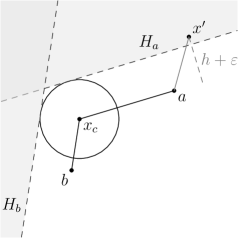
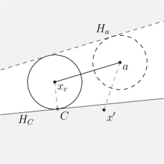
Figure 1. a) $P^{\prime}\subset H_{a}^{\complement}\cap H_{b}^{\complement}\cap H_{C}$,  b) ray $x_{c}$ to $a$ must meet $H_{C}$

Next, $H_{C}$ must be distance $h$ from $a$: if it were not, then for any $x^{\prime}\in P^{\prime}$ we have $d(a,x^{\prime})\geq d(a,H_{C})>h$ since $P^{\prime}\subset H_{C}$ as was shown above. Hence $\partial H_{C}$ and $\partial H_{a}$ are either parallel (a case we skip in this proof) or meet at a point $A^{\prime}$, in which case the ray from $x_{c}$ towards $a$ intersects $H_{C}$. Do the same for $b$ to get $B^{\prime}$. See Figure 1b. This means that $S(x_{c},h)$ is the incircle of the triangle formed by $H_{a}$, $H_{b}$ and $H_{C}$.

We can now see that $x_{c}$ is a vertex of $Q$. First of all $x_{c}\in\overline{Q}$ since $x_{c}\in\overline{P}$. Also, $P$ is inside the angle $ax_{c}b$ and $P^{\prime}$ inside the angle $A^{\prime}x_{c}B^{\prime}$, which is obviously less than $\pi$. Thus $x_{c}$ is a vertex of $Q$. Moreover its angle is at most $\angle A^{\prime}x_{c}B^{\prime}$. See Figure 2a.

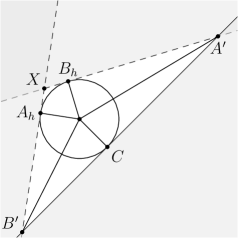
Figure 2. a) $S(x_{c},h)$ is an incircle,  b) solving $\angle A^{\prime}x_{c}B^{\prime}$

Let $X$ be the intersection of $\partial H_{a}$ and $\partial H_{b}$. This is a well-defined point since $0<\angle ax_{c}b<\pi$. We have $\angle A^{\prime}XB^{\prime}=\angle ax_{c}b=\alpha$ by parallel transport of $x_{c}a$ to $XA^{\prime}$ and $x_{c}b$ to $XB^{\prime}$. Let the perpendiculars from $x_{c}$ to $XA^{\prime}$, $A^{\prime}B^{\prime}$, $B^{\prime}X$ have base points $B_{h}$, $C$, $A_{h}$, respectively. See Figure 2b. Then $\angle A_{h}x_{c}B_{h}=\pi-\alpha$, $\angle B_{h}x_{c}A^{\prime}=\angle A^{\prime}x_{c}C$ and $\angle Cx_{c}B^{\prime}=\angle B^{\prime}x_{c}A_{h}$. This implies that $\angle A^{\prime}x_{c}B^{\prime}=(\alpha+\pi)/2$ at once since the sum of all of these angles is $2\pi$. ∎

Proof of Lemma 8.2.

The proof proceeds as in the proof of Lemma 8.1. We can choose coordinates such that $x_{c}=0$ and the three edges of $P$ starting from $x_{c}$ lie on the positive coordinate axes having unit vectors$e_{1}$, $e_{1}$ and $e_{3}$. Let $h=d(x_{c},C)=d_{H}(P,P^{\prime})$ for some $C\in\overline{P}^{\prime}$.

If we set $H_{j}=\{x\mid x\cdot e_{j}<-h\}$, then as in the 2D proof, we see that $P^{\prime}\subset H_{j}^{\complement}$. Similarly, if $H_{C}$ is the closed half-space tangent to $S(x_{c},h)$ at $C$, we see that $P^{\prime}\subset H_{C}$. Hence $P^{\prime}\subset H_{1}^{\complement}\cap H_{2}^{\complement}\cap H_{3}^{\complement}\cap H_{C}$.

If $C_{3}<0$, i.e. it is on the lower hemisphere of $S(x_{c},h)$, then there is $x\in P$ with $d(x,C)>h=d_{H}(P,P^{\prime})$. Just take any $x$ on the axis with $x_{3}>0$. The contradiction, seen also if $C_{1}<0$ or $C_{2}<0$, forces $C$ to be on the closed spherical triangle $T=\{x\mid\left\lvert x\right\rvert=1,x_{j}\geq 0\}$.

Now, no matter where $C\in T$ is, recalling that $P^{\prime}\subset H_{1}^{\complement}\cap H_{2}^{\complement}\cap H_{3}^{\complement}\cap H_{C}$, it is easy to see that

$$\sup_{A,B\in P\cup P^{\prime}}\angle Ax_{c}B<\pi$$

and hence that $H_{1}^{\complement}\cap H_{2}^{\complement}\cap H_{3}^{\complement}\cap H_{C}$ fits inside an spherical cone that does not contain a plane. Moreover the minimal required angle of the spherical cone depends continuously on the location of $C\in T$. Compactness of the latter implies the claim. ∎

10. Concluding remark

In this paper, we establish two sharp quantitative results for the direct and inverse time-harmonic acoustic wave scattering problem. The first one is a logarithmic stability result in recovering the support of an inhomogeneous medium, independent of its contents, by a single far-field measurement, which quantifies the uniqueness result in [22]. The second result shows that if an inhomogeneous medium possesses a corner, then it scatters an incident wave field stably in the sense that the energy of the corresponding scattered far-field possesses a positive lower bound. This quantifies the corner scattering result in [10] and has interesting implications to cloaking applications. Those topics are of fundamental importance in the wave scattering theory. In order to establish the quantitative results, we also make several technical new developments, which might be useful for tackling other direct and inverse scattering problems. Finally, we would like to remark that we only consider the case that the acoustic mediums are isotropic and it would be interesting and of practical importance to investigate the case that the inhomogeneous mediums are anisotropic. We are aware of a recent paper [11], where the authors studied the acoustic scattering from an anisotropic acoustic medium that possesses a corner. It is shown that an anisotropic corner can always scatter a nontrivial far-field pattern, which extends the study in [10] to the more challenging anisotropic case. The extension is technically highly nontrivial. It would be interesting to consider extending the quantitative studies in the current article to the anisotropic setting. We shall report our study in this aspect in our future work.

Since the post of this work to arXiv in 2016, there have been many developments in the literature on qualitatively and quantitatively characterizing the geometrical singularities in wave scattering as well as their implications to inverse problems and invisibility. Accordingly, we mention here [3, 4, 5, 6, 7, 8, 9], [12, 13] as well as a recent survey paper [29].

References

- [1] G. Alessandrini and L. Rondi, Determining a sound-soft polyhedral scatterer by a single far-field measurement, Proc. Amer. Math. Soc. 133 (2005), no. 6, 1685–1691.
- [2] A. Behzadan and M. Holst, Multiplication in Sobolev spaces, revisited, Ark. Mat. 59 (2021), no. 2, 275–306.
- [3] E. Blåsten, Nonradiating sources and transmission eigenfunctions vanish at corners and edges, SIAM J. Math. Anal. 50 (2018), no. 6, 6255–6270.
- [4] E. Blåsten, X. Li, H. Liu and Y. Wang, On vanishing and localizing of transmission eigenfunctions near singular points: a numerical study, Inverse Problems 33 (2017), no. 10, 105001, 24 pp.
- [5] E. Blåsten and Y.-H. Lin, Radiating and non-radiating sources in elasticity, Inverse Problems 35 (2019), no. 1, 015005, 16 pp.
- [6] E. Blåsten and H. Liu, On vanishing near corners of transmission eigenfunctions, J. Funct. Anal. 273 (2017), no. 11, 3616–3632.
- [7] E. Blåsten and H. Liu, Recovering piecewise constant refractive indices by a single far-field pattern, Inverse Problems 36 (2020), no. 8, 085005, 16 pp.
- [8] E. L. K. Blåsten and H. Liu, Scattering by curvatures, radiationless sources, transmission eigenfunctions, and inverse scattering problems, SIAM J. Math. Anal. 53 (2021), no. 4, 3801–3837.
- [9] E. Blåsten, H. Liu and J. Xiao, On an electromagnetic problem in a corner and its applications, Anal. PDE 14 (2021), no. 7, 2207–2224.
- [10] E. Blåsten, L. Päivärinta and J. Sylvester, Corners always scatter, Comm. Math. Phys. 331 (2014), no. 2, 725–753.
- [11] F. Cakoni and J. Xiao, On corner scattering for operators of divergence form and applications to inverse scattering, (2019), preprint, arXiv:1905.02558.
- [12] X. Cao, H. Diao and H. Liu, Determining a piecewise conductive medium body by a single far-field measurement, CSIAM Trans. Appl. Math. 1 (2020), no. 4, 740–765.
- [13] X. Cao, H. Diao and H. Liu, On the geometric structures of transmission eigenfunctions with a conductive boundary condition and applications, Comm. Partial Differential Equations 46 (2021), no. 4, 630–679.
- [14] H. Chen and C. T. Chan, Acoustic cloaking in three dimensions using acoustic metamaterials, Applied Physics Letters, 91 (2007), no. 18, 183518.
- [15] J. Cheng and M. Yamamoto, Uniqueness in an inverse scattering problem within non-trapping polygonal obstacles with at most two incoming waves, Inverse Problems 19 (2003), no. 6, 1361–1384.
- [16] D. Colton and R. Kress, Inverse acoustic and electromagnetic scattering theory, second edition, Applied Mathematical Sciences, 93, Springer-Verlag, Berlin, 1998.
- [17] D. Gilbarg and N. S. Trudinger, Elliptic partial differential equations of second order, second edition, Grundlehren der mathematischen Wissenschaften, 224, Springer-Verlag, Berlin, 1983.
- [18] A. Greenleaf, Y. Kurylev , M. Lassas and G. Uhlmann, Cloaking devices, electromagnetic wormholes, and transformation optics, SIAM Rev. 51 (2009), no. 1, 3–33.
- [19] A. Greenleaf, Y. Kurylev , M. Lassas and G. Uhlmann, Invisibility and inverse problems, Bull. Amer. Math. Soc. (N.S.) 46 (2009), no. 1, 55–97.
- [20] A. Greenleaf, M. Lassas and G. Uhlmann, On nonuniqueness for Calderón’s inverse problem, Math. Res. Lett. 10 (2003), no. 5-6, 685–693.
- [21] L. Hörmander, The analysis of linear partial differential operators. II, Grundlehren der mathematischen Wissenschaften, 257, Springer-Verlag, Berlin, 1983.
- [22] G. Hu, M. Salo and E. V. Vesalainen, Shape identification in inverse medium scattering problems with a single far-field pattern, SIAM J. Math. Anal. 48 (2016), no. 1, 152–165.
- [23] V. Isakov, Stability estimates for obstacles in inverse scattering, J. Comput. Appl. Math. 42 (1992), no. 1, 79–88.
- [24] V. Isakov, New stability results for soft obstacles in inverse scattering, Inverse Problems 9 (1993), no. 5, 535–543.
- [25] V. Isakov, Inverse problems for partial differential equations, second edition, Applied Mathematical Sciences, 127, Springer, New York, 2006.
- [26] C. E. Kenig, A. Ruiz and C. D. Sogge, Uniform Sobolev inequalities and unique continuation for second order constant coefficient differential operators, Duke Math. J. 55 (1987), no. 2, 329–347.
- [27] U. Leonhardt, Optical conformal mapping, Science 312 (2006), no. 5781, 1777–1780.
- [28] J. Li, H. Liu, L. Rondi and G. Uhlmann, Regularized transformation-optics cloaking for the Helmholtz equation: from partial cloak to full cloak, Comm. Math. Phys. 335 (2015), no. 2, 671–712.
- [29] H. Liu, On local and global structures of transmission eigenfunctions and beyond, Journal of Inverse and Ill-posed Problems (2020), 000010151520200099.
- [30] H. Liu, Virtual reshaping and invisibility in obstacle scattering, Inverse Problems 25 (2009), no. 4, 045006, 16 pp.
- [31] H. Liu, M. Petrini , L. Rondi and J. Xiao, Stable determination of sound-hard polyhedral scatterers by a minimal number of scattering measurements, J. Differential Equations 262 (2017), no. 3, 1631–1670.
- [32] H. Liu and H. Sun, Enhanced near-cloak by FSH lining, J. Math. Pures Appl. (9) 99 (2013), no. 1, 17–42.
- [33] H. Liu and G. Uhlmann, Regularized transformation-optics cloaking in acoustic and electromagnetic scattering, in Inverse problems and imaging, 111–136, Panor. Synthèses, 44, Soc. Math. France, Paris, 2015.
- [34] H. Liu and J. Zou, Uniqueness in determining multiple polygonal scatterers of mixed type, Discrete Contin. Dyn. Syst. Ser. B 9 (2008), no. 2, 375–396.
- [35] H. Liu and J. Zou, Uniqueness in an inverse acoustic obstacle scattering problem for both sound-hard and sound-soft polyhedral scatterers, Inverse Problems 22 (2006), no. 2, 515–524.
- [36] A. I. Nachman, Reconstructions from boundary measurements, Ann. of Math. (2) 128 (1988), no. 3, 531–576.
- [37] L. Päivärinta, M. Salo and E. V. Vesalainen, Strictly convex corners scatter, Rev. Mat. Iberoam. 33 (2017), no. 4, 1369–1396.
- [38] J. B. Pendry, D. Schurig and D. R. Smith, Controlling electromagnetic fields, Science 312 (2006), no. 5781, 1780–1782.
- [39] Rakesh and G. Uhlmann, Uniqueness for the inverse backscattering problem for angularly controlled potentials, Inverse Problems 30 (2014), no. 6, 065005, 24 pp.
- [40] Rakesh and G. Uhlmann, The point source inverse back-scattering problem, in Analysis, complex geometry, and mathematical physics: in honor of Duong H. Phong, 279–289, Contemp. Math., 644, Amer. Math. Soc., Providence, RI, 2015.
- [41] L. Rondi, Stable determination of sound-soft polyhedral scatterers by a single measurement, Indiana Univ. Math. J. 57 (2008), no. 3, 1377–1408.
- [42] L. Rondi and M. Sini, Stable determination of a scattered wave from its far-field pattern: the high frequency asymptotics, Arch. Ration. Mech. Anal. 218 (2015), no. 1, 1–54.
- [43] A. Ruiz, Harmonic Analysis and Inverse Problems, Lecture Notes, 2002, accessed 24.01.2018.
- [44] J. Sylvester and G. Uhlmann, A global uniqueness theorem for an inverse boundary value problem, Ann. of Math. (2) 125 (1987), no. 1, 153–169.
- [45] H. Triebel, Theory of function spaces, Monographs in Mathematics, 78, Birkhäuser Verlag, Basel, 1983.
- [46] H. Triebel, Theory of function spaces. II, Monographs in Mathematics, 84, Birkhäuser Verlag, Basel, 1992.
- [47] G. Uhlmann, Visibility and invisibility, in ICIAM 07—6th International Congress on Industrial and Applied Mathematics, 381–408, Eur. Math. Soc., Zürich, 2009.
- [48] G. Uhlmann, editor, Inverse problems and applications: inside out. II, Mathematical Sciences Research Institute Publications, 60, Cambridge University Press, Cambridge, 2013.