Several different analysis methods have been developed to determine the strong coupling via finite-energy sum-rule analyses of hadronic $\tau$ decay data. While most methods agree on the existence of the well-known ambiguity in the choice of a resummation scheme due to the slow convergence of QCD perturbation theory at the $\tau$ mass, there is an ongoing controversy over how to deal properly with non-perturbative effects. These are small, but not negligible, and include quark-hadron “duality violations” (i.e., resonance effects) which are not described by the operator product expansion (OPE). In one approach, an attempt is made to suppress duality violations enough that they might become negligible. The number of OPE parameters to be fit, however, then exceeds the number of available sum rules, necessitating an uncontrolled OPE truncation, in which a number of higher-dimension OPE contributions in general present in QCD are set to zero by hand. In the second approach, truncation of the OPE is avoided by construction, and duality violations are taken into account explicitly, using a physically motivated model. In this article, we provide a critical appraisal of a recent analysis employing the first approach and demonstrate that it fails to properly account for non-perturbative effects, making the resulting determination of the strong coupling unreliable. The second approach, in contrast, passes all self-consistency tests, and provides a competitive determination of the strong coupling from $\tau$ decays.

I Introduction

A precise determination of the strong coupling $\alpha_{s}$ is important, both because it is one of the fundamental parameters of the Standard Model, and because it is an important input to precision studies of potential discrepancies between experiment and theory, relevant to searches for beyond-the-Standard-Model physics. Moreover, determinations over a wide range of energies provide an important test of the running of the coupling as predicted by QCD.

Experimental data for hadronic $\tau$ decays provide an opportunity for a determination at quite low energy scales, of order the $\tau$ mass. Because of the long running from the $\tau$ mass to the $Z$ mass, even a modestly accurate determination translates into a high-precision value at the $Z$ mass, and, as such, provides a stringent test of QCD. However, $\alpha_{s}$ is, of course, defined in perturbation theory, and it is thus imperative to have a quantitative understanding of non-perturbative effects that may “contaminate” determinations at lower scales such as that at the $\tau$ mass, where resonance effects are clearly visible in the QCD spectral functions extracted from differential $\tau$ decay distributions. Such resonance effects, which are described neither by perturbation theory nor by the operator product expansion (OPE), are referred to generically in the literature as “violating quark-hadron duality.” A quantitative study of the impact of duality violations (DVs) is unavoidable if one aims to fully understand the possible systematics affecting the extraction of $\alpha_{s}(m_{\tau}^{2})$ from $\tau$ decays.

Two basic strategies have been developed to extract $\alpha_{s}(m_{\tau}^{2})$ from hadronic $\tau$ decay data. Both are based on the use of finite-energy sum rules (FESRs), in which weighted integrals of the vector ($V$) and axial-vector ($A$) hadronic spectral functions (or their sum) are related to the integral on a circle around the origin in the complex plane over a theoretical representation of the $V$ or $A$ current two-point function. Choosing the radius $s_{0}$ of this circle to be large makes it possible to use perturbation theory, augmented by the OPE and possibly also with a model for residual DVs, for the theoretical representation, allowing for the extraction of $\alpha_{s}(s_{0})$. Of course, in the application of FESRs to $\tau$ decays, the maximum radius is $s_{0}=m_{\tau}^{2}$.

In the first strategy, the weights in the spectral integrals are chosen with the hope of suppressing DVs enough to justify omitting them from the analysis, and, in this spirit, $s_{0}$ is always chosen equal to its maximum kinematically allowed value, $m_{\tau}^{2}$. As we will see, in order to keep the number of the resulting sum rules greater than the number of parameters to be fit, this choice forces a truncation of the OPE at a dimension lower than a complete QCD analysis would generally require. We will refer to this strategy as the “truncated-OPE-model” or “truncated-OPE” strategy. The most recent implementations of this strategy can be found in Refs. ALEPH13 ; Pich .

In the second strategy, weights are chosen such that only low orders in the OPE need to be included. It turns out that this is incompatible with the desired complete suppression of DVs, and an explicit model of how they affect the spectral functions needs to be introduced in order to carry out the analysis. The value of $s_{0}$ is varied between approximately $1.5$ GeV² and $m_{\tau}^{2}$. This approach has been followed in Refs. alphas1 ; alphas2 ; alphas14 , and we will refer to it as the “DV-model strategy.”

Both strategies are based on assumptions, and these assumptions have to be tested. This is not an academic issue, because the values of $\alpha_{s}(m_{\tau}^{2})$ obtained by applying the two different strategies to the same data set differ significantly, the DV-model result being lower by about $8\%$. This difference is a factor of two larger than the $4\%$ (or less) errors produced using the individual strategies.

The goal of this article is to present a critical analysis of the truncated-OPE-model strategy, starting from the extensive analysis recently presented in Ref. Pich . In Ref. Pich a large number of tests of this strategy were carried out, leading to the claim that the strategy is robust, even if there is no good a priori physical motivation for the truncation of the OPE employed. Here we will demonstrate that despite these tests, this strategy does not, in fact, hold up, and that consequently the final result for $\alpha_{s}(m_{\tau}^{2})$ obtained in Refs. ALEPH13 ; Pich is unreliable. In particular, while the tests carried out in Ref. Pich are certainly necessary, they are not sufficient to be confident that the systematic errors quoted in Ref. Pich , following from the use of this strategy, are under control. In what follows, we will show explicitly that they are not.

Of course, the DV-model strategy requires similar scrutiny, and numerous self-consistency tests have already been carried out in Refs. alphas1 ; alphas2 ; alphas14 . The details of these tests will not be repeated here, but may be found in those references. As we will argue below, the deficiencies of the truncated-OPE-model strategy in fact naturally lead one to adopt the DV-model strategy, a point already made in some detail in Ref. alphas1 . We will also show that the criticism of the DV-model strategy in Ref. Pich is misleading, and in fact in no way invalidates the DV-model strategy approach.

This article is organized as follows. In the next section, we collect elements of the theory of FESRs needed for our purposes. Then, in Sec. III, we begin by reproducing the results of Ref. Pich , and end with a discussion of hints of instabilities already visible in these results. In Sec. IV, we carry out a numerical experiment using fake data which are compatible with the experimental spectral functions, and which have been generated from a model of the $V$ and $A$ spectral functions with fixed input $\alpha_{s}(m_{\tau}^{2})$ and, by construction, non-negligible DVs. We show that fits extracting $\alpha_{s}(m_{\tau}^{2})$ from these data employing the truncated-OPE strategy fail to reproduce the exactly known model value of $\alpha_{s}(m_{\tau}^{2})$ by an amount comparable to the difference found when the two strategies are applied to the real data. In Sec. V we refute the critique of the DV-model strategy contained in Ref. Pich . Section VI contains our conclusions.

II Theory

The sum-rule analysis underlying both strategies starts from the current-current two-point functions

$$\Pi_{\mu\nu}(q) = i\int d^{4}x\,e^{iqx}\langle 0|T\left\{J_{\mu}(x)J^{\dagger}_{\nu}(0)\right\}|0\rangle$$

$$= \left(q_{\mu}q_{\nu}-q^{2}g_{\mu\nu}\right)\Pi^{(1)}(q^{2})+q_{\mu}q_{\nu}\Pi^{(0)}(q^{2})$$

$$= \left(q_{\mu}q_{\nu}-q^{2}g_{\mu\nu}\right)\Pi^{(1+0)}(q^{2})+q^{2}g_{\mu\nu}\Pi^{(0)}(q^{2})\ ,$$

where $J_{\mu}$ is the non-strange $V_{\mu}=\overline{u}\gamma_{\mu}d$ or $A_{\mu}=\overline{u}\gamma_{\mu}\gamma_{5}d$ current, and the superscripts $(0)$ and $(1)$ label spin. The combinations $\Pi^{(1+0)}(q^{2})$ and $q^{2}\Pi^{(0)}(q^{2})$ are free of kinematic singularities. Defining $s=q^{2}=\,-Q^{2}$ and the spectral function

$$\rho^{(1+0)}(s)=\frac{1}{\pi}\;\mbox{Im}\,\Pi^{(1+0)}(s)\ ,$$ (2)

Cauchy’s theorem applied to the contour in Fig. 1 and the analytical properties of $\Pi^{(1+0)}(s)$ imply the FESR

$$\frac{1}{s_{0}}\int_{0}^{s_{0}}ds\,w(s/s_{0})\,\rho^{(1+0)}_{V/A}(s) = -\frac{1}{2\pi i\,s_{0}}\oint_{|s|=s_{0}}ds\,w(s/s_{0})\,\Pi^{(1+0)}_{V/A}(s)\ .$$ (3)

This FESR is valid for any $s_{0}>0$ and any weight $w(s)$ analytic inside and on the contour shankar ; Braaten88 ; BNP . It holds for the $V$ and $A$ cases separately, and as a consequence also for $V+A$.

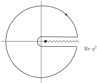
Figure 1: Analytic structure of $\Pi^{(1+0)}(q^{2})$ in the complex $s=q^{2}$ plane. There is a cut on the positive real axis starting at $s=q^{2}=4m_{\pi}^{2}$ (a pole at $s=q^{2}=m_{\pi}^{2}$ and a cut starting at $s=9m_{\pi}^{2}$) for the $V$ ($A$) case. The solid curve shows the contour used in Eq. (3).

Experimental results for the flavor $ud$ $V$ and $A$ spectral functions have been made available by ALEPH and OPAL in Refs. ALEPH13 ; ALEPH ; OPAL . Apart from the pion-pole contribution, $\rho_{V/A;ud}^{(0)}(s)=O[(m_{d}\mp m_{u})^{2}]$ is chirally suppressed, and the continuum part of $\rho_{V/A}^{(0)}(s)$ is thus numerically negligible.

For large $|s|=s_{0}$, and far enough away from the positive real axis, $\Pi^{(1+0)}(s)$ can be approximated by the OPE

$$\Pi^{(1+0)}_{\rm OPE}(s)=\sum_{k=0}^{\infty}\frac{C_{2k}(s)}{(-s)^{k}}\ .$$ (4)

We will omit the labels $V$, $A$ or $V+A$ on the OPE coefficients, because we will only encounter the case $V+A$ in this article. The $C_{2k}$ are logarithmically dependent on $s$ through perturbative corrections. The term with $k=0$ corresponds to the purely perturbative, mass-independent contributions, which have been calculated to order $\alpha_{s}^{4}$ in Ref. PT , and are the same for the $V$ and $A$ channels. Values quoted for $\alpha_{s}(m_{\tau}^{2})$ are in the $\overline{\rm MS}$ scheme. We will consider both FOPT and CIPT CIPT resummation schemes in evaluating the truncated perturbative series (see for instance Refs. MJ ; BJ for a discussion of these two resummation schemes). The $C_{2k}$ with $k\geq 1$ are different for the $V$ and $A$ channels, and, for $k>1$, contain non-perturbative $D=2k$ condensate contributions. As in Refs. ALEPH13 ; Pich ; alphas1 ; alphas2 ; alphas14 , we will neglect purely perturbative quark-mass contributions to $C_{2}$ and $C_{4}$, as they are numerically very small for the non-strange FERSs under consideration. We will also neglect the $s$-dependence of the coefficients $C_{2k}$ for $k>1$, because they are $\alpha_{s}$ suppressed. With this choice, we have that

$$\frac{1}{2\pi is_{0}}\oint_{|s|=s_{0}}\,ds\,\left(\frac{s}{s_{0}}\right)^{n}\,\frac{C_{2k}}{(-s)^{k}}=(-1)^{n+1}\frac{C_{2(n+1)}}{s_{0}^{n+1}}\,\delta_{k,n+1}\ ,$$ (5)

implying that an $n$-th degree monomial in the weight $w(s/s_{0})$ selects the $D=2k=2(n+1)$ term in the OPE.

All fit results for the $1/s^{4}$ term in the OPE will be given in terms of $C_{4}$, while Ref. Pich chose to use the gluon condensate, $\langle\frac{\alpha_{s}}{\pi}GG\rangle$, instead. For the $V+A$ case, these two parameters are related by

$$C_{4}=\frac{1}{6}\left(1-\frac{11}{18}\frac{\alpha_{s}}{\pi}\right)\left\langle\frac{\alpha_{s}}{\pi}GG\right\rangle+2\left(1-\frac{23}{27}\frac{\alpha_{s}}{\pi}\right)\langle(m_{u}+m_{d}){\overline{q}}q\rangle\ .$$ (6)

If we employ, as in Ref. Pich , the value $\langle(m_{u}+m_{d}){\overline{q}}q\rangle\approx-m_{\pi}^{2}f_{\pi}^{2}\approx-1.6\times 10^{-4}$ GeV⁴ with $\alpha_{s}\approx 0.325$, Eq. (6) translates into

$$C_{4}=0.156\,\left\langle\frac{\alpha_{s}}{\pi}GG\right\rangle-0.000292\ \mbox{GeV}^{4}\ .$$ (7)

Perturbation theory, and, more generally, the OPE, breaks down near the positive real axis PQW . In order to account for this, we replace the right-hand side of Eq. (3) by

$$-\frac{1}{2\pi is_{0}}\oint_{|s|=s_{0}}ds\,w(s/s_{0})\,\left(\Pi^{(1+0)}_{\rm OPE}(s)+\Delta(s)\right)\ ,$$ (8)

with

$$\Delta(s)\equiv\Pi^{(1+0)}(s)-\Pi^{(1+0)}_{\rm OPE}(s)\ ,$$ (9)

where the difference $\Delta(s)$ represents, by definition, the quark-hadron duality violating contribution to $\Pi^{(1+0)}(s)$. As shown in Ref. CGP , the integral over $w(s/s_{0})\Delta(s)$ in Eq. (8) can be rewritten such that the FESR takes the form

$$\frac{1}{s_{0}}\int_{0}^{s_{0}}ds\,w(s/s_{0})\,\rho^{(1+0)}_{V/A}(s)$$ (10)

$$=-\frac{1}{2\pi is_{0}}\oint_{|s|=s_{0}}ds\,w(s/s_{0})\,\Pi^{(1+0)}_{{\rm OPE},V/A}(s)-\frac{1}{s_{0}}\,\int_{s_{0}}^{\infty}ds\,w(s/s_{0})\,\frac{1}{\pi}\,\mbox{Im}\,\Delta_{V/A}(s)\ ,$$

if $\Delta(s)$ is assumed to decay fast enough as $s\to\infty$. The imaginary parts $\frac{1}{\pi}\,\mbox{Im}\,\Delta_{V/A}(s)$ can thus be interpreted as the duality-violating parts, $\rho_{V/A}^{\rm DV}(s)$, of the $V/A$ spectral functions.

We need to resort to a model in order to account for DVs, because the functional form of $\Delta(s)$ is not known, even for large $s$. As in Refs. CGP ; CGPmodel ; CGP05 , our model is based on large-$N_{c}$ and Regge considerations, parametrizing $\rho_{V/A}^{\rm DV}(s)$ as

$$\rho_{V/A}^{\rm DV}(s)=e^{-\delta_{V/A}-\gamma_{V/A}s}\sin{(\alpha_{V/A}+\beta_{V/A}s)}\ ,\qquad s\geq s_{\rm min}\ .$$ (11)

This introduces four new parameters in each channel, in addition to $\alpha_{s}$ and the $D\geq 4$ OPE coefficients. Our ansatz (11) is assumed to hold only for $s\geq s_{\rm min}$, with $s_{\rm min}$ to be determined from fits to the data. We emphasize that, since DVs represent resonance effects, the DV parameters will be different in the $V$ and $A$ channels, reflecting the different resonance structure in these two channels.

One way the general structure of the ansatz proposed in Eq. (11) can be understood is as follows. The OPE itself diverges as an expansion in $1/s$, because it has zero radius of convergence around $1/s=0$. It is thus itself, like the perturbative series in the $D=0$ term MB , at best an asymptotic expansion, with coefficients $C_{2k}$ that must eventually grow rapidly with $k$. This then leads to the expectation that an exponential correction suppressed in terms of the inverse of this expansion parameter, “takes over” where the OPE starts to diverge. The form given in Eq. (11) is consistent with this expectation. Moreover, following this line of reasoning, it would be natural to expect that the prefactor of the form (11) is itself an expansion in powers of $1/s$. In ansatz (11) only the leading (constant) term was kept in this prefactor expansion.

III The truncated-OPE-model strategy

In this section, we will first summarize the truncated-OPE strategy of Ref. Pich . We will then, after reproducing the results of Ref. Pich in Sec. III.1, start a critical discussion of both these results and the underlying strategy in Sec. III.2.

The orginal version DP1992 of the truncated-OPE strategy employed five different FESRs, corresponding to five different polynomial choices for the weight function $w(x)$ in the FESR (3). We will denote these weights as $w_{k\ell}$, with $(k\ell)\in\{(00),(10),(11),(12),(13)\}$, and

$$w_{k\ell}(x)=(1-x)^{k+2}x^{\ell}(1+2x)\ .$$ (12)

These weights have a double or triple zero at $s=s_{0}$ (i.e., $x=1$), and the hope was that this would be sufficient to suppress DVs enough that they could be neglected. In other words, in all the fits of Ref. Pich all weighted integrals of the functions $\rho^{\rm DV}_{V/A}(s)$ of Eq. (11) are set equal to zero. In practice, this is equivalent to choosing a model in which $\rho^{\rm DV}_{V/A}(s)=0$, i.e., $\delta_{V/A}=\infty$, from the outset, regardless of the oscillations clearly visible in Fig. 2. The value of $s_{0}$ was chosen equal to $m_{\tau}^{2}$, again with the hope that this would maximize the suppression of non-perturbative effects represented by the $D=2k>0$ terms in the OPE, Eq. (4), and $\Delta(s)$, Eq. (9). Prima facie, this is not an implausible assumption, as perturbation theory should provide an approximation to the right-hand side of Eq. (3) that becomes more accurate as $s_{0}$ increases.

These choices imply that one has five data points, and one thus needs to limit the number of parameters in the fit to four (or less). This leads to the necessity of truncating the OPE. Since $C_{2}$ is negligibly small for the non-strange channels considered here, the choice was made to take $\alpha_{s}(m_{\tau}^{2})$, $C_{4}$, $C_{6}$ and $C_{8}$ as free parameters in the fit. However, because of Eq. (5), this amounts to the additional assumption that $C_{10}=C_{12}=C_{14}=C_{16}=0$, since the set Eq. (12) contains polynomials with degree up to seven. While such an assumption is necessary to implement the chosen fit strategy, it has no basis in QCD.

In addition to the set of weights in Eq. (12), Ref. Pich considered several other sets of polynomials in $x$, in order to test this strategy.

In one set, which we refer to as the “reduced set”, denoted $w_{k\ell}^{\rm red}(x)$, the factor $1+2x$ was removed from the $w_{k\ell}$. The form of the weights $w_{k\ell}^{\rm red}(x)$ is then

$$w^{\rm red}_{k\ell}(x)=(1-x)^{k+2}x^{\ell}\ .$$ (13)

Again, the pair $(kl)$ was chosen in the set $\{(00),(10),(11),(12),(13)\}$. The motivation for this choice is that it “reduces” the number of assumptions associated with the chosen OPE truncation; one needs only assume $C_{10}=C_{12}=C_{14}=0$, since $C_{16}$ is not probed by this modified set. Other sets of weights can be chosen from among the “optimal” weights $w_{m,n}^{\rm opt}(x)$, where

$$w^{\rm opt}_{m,n}=(1-x)^{1+m}\left(\frac{d~{}}{dx}\right)^{m}\sum_{k=0}^{n}x^{m+k}\ ,\qquad m=0,1\ ,\qquad n=1,\dots,5\ .$$ (14)

For $m=0$ each of these weights selects only one $D>0$ term in the OPE, and for $m=1$ each of these weights selects only two $D>0$ terms. The $m=0$ “optimal” weights are singly pinched and the $m=1$ “optimal” weights are doubly pinched. The most important of these weights are those with $m=1$, because they are doubly pinched, and, for $n\geq 1$ the two OPE terms probed by these weights have $D\geq 6$, thus avoiding a contribution from the nominally dominant $D=4$ term. The $m=0$ weights probe only one term in the OPE, but are expected to be less effective in suppressing DVs because they are only singly pinched. For the set with $m=1$ and $1\leq n\leq 5$, the truncation assumption amounts to setting $C_{12}=C_{14}=C_{16}=0$.

Yet another set of weights considered was the four-weight set, $w_{n}(x)$, $n=0,\dots,3$, with

$$w_{n}(x)=(1-x)^{n}\ .$$ (15)

For this set, the parameters $\alpha_{s}(m_{\tau}^{2})$, $C_{4}$ and $C_{6}$ were fit, while the OPE was truncated by setting $C_{8}=0$ in order to have one degree of freedom in the fit, even though $C_{8}$ is probed by $w_{3}$. This set is a little different in nature, because $w_{0}$ is unpinched, and $w_{1}$ is only singly pinched. Therefore, the effects from DVs are potentially more severe.

The truncation assumption affects the higher-degree weights more. For example, $w_{00}=w^{\rm opt}_{1,1}$ is not affected, because it only probes OPE terms with $D\leq 8$, $w_{10}$ and $w^{\rm opt}_{1,2}$ only probe in addition the $D=10$ term, etc. This could lead one to hope that, despite the fact that the assumed truncation has no ground in QCD, the determination of $\alpha_{s}$ might be less severely affected. This could, for example, happen if the spectral moments involving lower-degree weights are relatively more important in fixing $D=0$ contributions than are those involving higher-degree weights. Any such speculation should, of course, be explicitly tested. While Ref. Pich carried out a number of such tests (which we will also consider below), we will nevertheless see that the truncation assumption employed in the truncated-OPE strategy has a significant impact on the value of $\alpha_{s}$ obtained from this collection of fits. In other words, though the many tests in Ref. Pich can be considered as necessary, they turn out not to be sufficient.

III.1 Reproduction of the fits of Ref. Pich

Before we investigate the validity of the truncated-OPE strategy, we first reproduce the fits of Ref. Pich based on this strategy. We will only consider fits to moments computed from the sum of the $V$ and $A$ non-strange spectral functions, as Ref. Pich advocates that this is the most reliable choice. We primarily consider fits using the four sets of weights specified above, and our version of the results is reported in Tables 1, 2, 3 and 4 below.

These are all good fits, and the results agree with those found in Ref. Pich , within our statistical errors. Since our goal is not to obtain final results for $\alpha_{s}$ from these fits, we do not repeat the estimates of systematic errors carried out in Ref. Pich . We note that the central values are slightly different. This is most likely due to a slightly different treatment of the data, including a small rescaling performed in Ref. alphas14 . Using Eq. (7), it is straightforward to verify that our values for $C_{4}$ are consistent with the values for $\langle\frac{\alpha_{s}}{\pi}GG\rangle$ given in Ref. Pich . We verified the results found in Table 5 of Ref. Pich as well, with similar accuracy. We do not show these here, since they are less central to the final value for $\alpha_{s}(m_{\tau}^{2})$ quoted in Ref. Pich .

	$\alpha_{s}(m_{\tau}^{2})$	$C_{4}$ (GeV4)	$C_{6}$ (GeV6)	$C_{8}$ (GeV8)	$\chi^{2}/$dof
FOPT	0.316(3)	-0.0006(3)	0.0012(3)	-0.0008(3)	1.38/1
CIPT	0.336(4)	-0.0026(4)	0.0009(3)	-0.0010(4)	0.89/1

Table 1: Reproduction of the $V+A$ fits of Table 1 of Ref. Pich , based on the weights of Eq. (12). By assumption, $C_{10}=C_{12}=C_{14}=C_{16}=0$. Errors are statistical only.

	$\alpha_{s}(m_{\tau}^{2})$	$C_{4}$ (GeV4)	$C_{6}$ (GeV6)	$C_{8}$ (GeV8)	$\chi^{2}/$dof
FOPT	0.316(2)	-0.0005(1)	0.0011(1)	-0.0005(1)	1.57/1
CIPT	0.336(4)	-0.0025(3)	0.0008(2)	-0.0008(2)	0.98/1

Table 2: Reproduction of the $V+A$ fits of Table 3 of Ref. Pich , based on the reduced weights (13). By assumption, $C_{10}=C_{12}=C_{14}=0$. Errors are statistical only.

	$\alpha_{s}(m_{\tau}^{2})$	$C_{6}$ (GeV6)	$C_{8}$ (GeV8)	$C_{10}$ (GeV10)	$\chi^{2}/$dof
FOPT	0.317(3)	0.0014(4)	-0.0010(5)	0.0004(3)	1.26/1
CIPT	0.336(4)	0.0010(4)	-0.0011(5)	0.0003(3)	0.83/1

Table 3: Reproduction of the $V+A$ fits of Table 7 of Ref. Pich , based on the “optimal” weights (14) with $m=1$ and $n=1,\dots\,5$. By assumption, $C_{12}=C_{14}=C_{16}=0$. Errors are statistical only.

	$\alpha_{s}(m_{\tau}^{2})$	$C_{4}$ (GeV4)	$C_{6}$ (GeV6)	$\chi^{2}/$dof
FOPT	0.320(8)	-0.001(1)	0.002(2)	1.25/1
CIPT	0.339(11)	-0.003(3)	0.001(2)	1.15/1

Table 4: Reproduction of the $V+A$ fits of Table 6 of Ref. Pich , based on the weights of Eq. (15) with $n=0,\dots\,3$. By assumption, $C_{8}=0$. Errors are statistical only.

III.2 Critique

We will now turn to a discussion of observations on the basic assumptions underlying the truncated-OPE-model strategy, based on the data. First, we consider the OPE truncation itself, then investigate the other key assumption that, at the $\tau$ scale, double (or triple) pinching produces a suppression of DV contributions strong enough to allow them to be ignored.

III.2.1 Truncation of the OPE

To obtain the results reported in Tables 1 to 4 above, two major assumptions have been made. The first is that setting to zero by hand higher-dimension OPE contributions in principle present in the analysis (unavoidable if one wishes to have at least one degree of freedom in the fit) has no significant impact on the resulting $\alpha_{s}(m_{\tau}^{2})$. This assumption was tested in Ref. Pich by relaxing this constraint on the coefficient $C_{D}$ with $D$ equal to the lowest dimension of the OPE term neglected in the fits described in Sec. III.1. For the fits of Table 1 and 2 this means that now also $C_{10}$ is left as a free parameter, while for Table 3 the corresponding new free parameter is $C_{12}$. Of course, now we have no degrees of freedom left, the minimal value of $\chi^{2}$ is zero, and these tests are not proper fits. Nonetheless, errors on the free parameters can still be found through linear error propagation, and these results can thus be compared with the results reported in Sec. III.1.

Here, let us reproduce the first example of these tests. We again carry out a “fit” to the spectral-function integrals with weights (12), but now use these to determine the parameters $\alpha_{s}$, $C_{4,6,8}$ and $C_{10}$. Our results are reported in Table 5.

	$\alpha_{s}(m_{\tau}^{2})$	$C_{4}$ (GeV4)	$C_{6}$ (GeV6)	$C_{8}$ (GeV8)	$C_{10}$ (GeV10)
FOPT	0.329(12)	-0.0014(8)	0.005(4)	-0.004(3)	0.010(8)
CIPT	0.350(15)	-0.0036(12)	0.004(3)	-0.004(3)	0.007(8)

Table 5: Reproduction of the $V+A$ “fits” of Table 2 of Ref. Pich , based on the weights of Eq. (12), to be compared with Table 1. By assumption, $C_{12}=C_{14}=C_{16}=0$, while $C_{10}$ is now left as a free parameter. Errors are obtained through linear error propagation.

These results are in agreement with Table 2 of Ref. Pich , within errors. They are also in agreement within errors with Table 1. Ref. Pich takes this as a sign of stability of the fits of Table 1, and thus as a validation of the truncation of the OPE beyond the $D=8$ term. However, while the errors on the coefficients $C_{6}$ and $C_{8}$ are large, so that there is no inconsistency between the values of these parameters obtained in Tables 1 and 5, one notes that their central values in Table 5 are roughly five times as large as those of Table 1. We also note that the central values of $\alpha_{s}(m_{\tau}^{2})$ in Table 5 are larger than in Tables 1 to 4. Similar observations hold for similar “fits” with no degrees of freedom with reduced and “optimal” weights, cf. Tables 4 and 8 in Ref. Pich . This suggests that the OPE coefficients may “want” to be larger, but that just adding one more term in the fit, while still truncating the remaining terms, does not allow the OPE the “room” to do this. As we will see below, reasonable values for the OPE condensates exist which are compatible with the data, but which lead to significantly lower values of $\alpha_{s}$. The tests carried out in Ref. Pich , and given in their Tables 2, 4 and 8, are thus, in fact, inconclusive.

Interestingly, no such test was carried out for the fits of Table 6 in Ref. Pich , which we reproduce here in Table 4. Such a test can, of course, be performed by leaving $C_{8}$ as a free parameter. We carried out this test, and find the values in Table 6 below. We note that there is a very dramatic shift in the central value of $\alpha_{s}(m_{\tau}^{2})$, of about 24%, while also the errors increase dramatically. Taken all together, we conclude that tests based on “fits” with zero degrees of freedom add no information, and are certainly not a demonstration of stability of the truncated-OPE strategy.

	$\alpha_{s}(m_{\tau}^{2})$	$C_{4}$ (GeV4)	$C_{6}$ (GeV6)	$C_{8}$ (GeV8)
FOPT	0.39(6)	-0.02(3)	0.07(8)	-0.2(2)
CIPT	0.43(10)	-0.03(3)	0.06(6)	-0.2(2)

Table 6: Test of the $V+A$ “fits” of Table 6 of Ref. Pich , based on the weights of Eq. (15), to be compared with Table 4. $C_{8}$ is now left as a free parameter. Errors are obtained through linear error propagation.

We now will consider an exercise which shows that the whole collection of fits carried out in Ref. Pich admits a very different solution. This will serve to demonstrate that the argument of Ref. Pich , that the consistency of the results obtained from all the tests performed there establishes the robustness of the determination of $\alpha_{s}$, is false.

Let us return to the fits of Tables 1 to 4. Since the choice of setting any of the OPE coefficients equal to zero is arbitrary, one might consider a different set, which, at this point, may also seem rather arbitrary:

$$C_{8} = 0.0349\ \mbox{GeV}^{8}\ ,$$ (16)

$$C_{10} = -0.0832\ \mbox{GeV}^{10}\ ,$$

$$C_{12} = 0.161\ \mbox{GeV}^{12}\ ,$$

$$C_{14} = -0.17\ \mbox{GeV}^{14}\ ,$$

$$C_{16} = -0.55\ \mbox{GeV}^{16}\ .$$

Even if arbitrary, this choice for $C_{D}$ with $8\leq D\leq 16$ is a reasonable one. The values are of the order or magnitude one might expect in QCD, with its typical hadronic scale of about 1 GeV. Measured in units of 1 GeV, they increase with $D$, but also this is not excluded or unnatural, if indeed the OPE is an asymptotic series (cf. Sec. II).

Redoing the fits of Tables 1 to 4, but now with Eq. (16) as input, we find the results presented in Tables 7 to 10.

	$\alpha_{s}(m_{\tau}^{2})$	$C_{4}$ (GeV4)	$C_{6}$ (GeV6)	$C_{8}$ (GeV8)	$\chi^{2}/$dof
FOPT	0.295(3)	0.0043(3)	-0.0128(3)	0.0355(3)	0.99/1
CIPT	0.308(4)	0.0031(3)	-0.0129(3)	0.0354(3)	0.74/1

Table 7: Fits as in Table 1, but with $C_{10}$, $C_{12}$, $C_{14}$ and $C_{16}$ as given in Eq. (16). Errors are statistical only.

	$\alpha_{s}(m_{\tau}^{2})$	$C_{4}$ (GeV4)	$C_{6}$ (GeV6)	$C_{8}$ (GeV8)	$\chi^{2}/$dof
FOPT	0.296(3)	0.0042(2)	-0.0127(2)	0.0352(2)	0.84/1
CIPT	0.309(4)	0.0030(3)	-0.0128(2)	0.0351(2)	0.60/1

Table 8: Fits as in Table 2, but with $C_{10}$, $C_{12}$ and $C_{14}$ as given in Eq. (16). Errors are statistical only.

	$\alpha_{s}(m_{\tau}^{2})$	$C_{6}$ (GeV6)	$C_{8}$ (GeV8)	$C_{10}$ (GeV10)	$\chi^{2}/$dof
FOPT	0.295(4)	-0.0130(4)	0.0356(5)	-0.0836(3)	1.09/1
CIPT	0.308(5)	-0.0130(4)	0.0355(5)	-0.0836(3)	0.84/1

Table 9: Fits as in Table 3, but with $C_{12}$, $C_{14}$ and $C_{16}$ as given in Eq. (16). Errors are statistical only.

	$\alpha_{s}(m_{\tau}^{2})$	$C_{4}$ (GeV4)	$C_{6}$ (GeV6)	$\chi^{2}/$dof
FOPT	0.308(8)	0.0023(12)	-0.009(2)	1.73/1
CIPT	0.322(11)	0.0009(15)	-0.010(2)	1.63/1

Table 10: Fits as in Table 4, but with $C_{8}$ as given in Eq. (16). Errors are statistical only.

The fits of Tables 7 to 9 are all very good fits, as measured by their $\chi^{2}$ values, certainly at least as good as those of Tables 1 to 3. The implication of this exercise is that there could be at least two solutions, depending on what one assumes for the values of higher-dimension OPE coefficients. The existence of these two (and possibly more) solutions reveals a fundamental problem of the truncated-OPE strategy: the solution found by this strategy depends on the choice of the values of the OPE coefficients not included in the fits. In addition, the strategy does not provide a physics argument, either a priori or a posteriori, for what choice to make. The solution with Eq. (16) as input leads to values of $\alpha_{s}(m_{\tau}^{2})$ that are about 0.025, or 8%, lower than those obtained using the alternate input set in which the relevant higher-dimension $C_{D}$ are set to zero by hand. We note that the values for $C_{10}$ in Table 9, and $C_{8}$ in Tables 7 to 9, for which these coefficients are not input, agree well with the value in Eq. (16). Likewise, if one explores tests like those of Table 5, the results are internally consistent as well as consistent with the values in Eq. (16). Without further information, it is not possible to claim that one solution is better than the other. To summarize: the internal consistency among all fits cannot be used as a reliable test for judging the robustness of the result for $\alpha_{s}(m_{\tau}^{2})$, in contrast to what is advocated in Ref. Pich , because the solution described in this subsection passes all the same consistency tests.

We also considered the “secondary” tests of Tables 5 and 9 of Ref. Pich . In Table 5 of Ref. Pich the twelve moments with weights (14) were employed choosing $m=0,\ 1$, $n=0,\dots,5$, and $s_{0}=2.8$ GeV². For each moment a value of $\alpha_{s}(m_{\tau}^{2})$ was extracted ignoring all non-perturbative contributions, i.e., setting all $C_{D\geq 2}=0$ and ignoring DVs. While the results appeared to suggest self-consistency and consistency with all other fits, we found that this is only the case because Ref. Pich limits itself to the single choice $s_{0}=2.8$ GeV².

Since $s_{0}=2.6$ GeV² corresponds to the bin immediately before $s_{0}=2.8$ GeV², we have varied $s_{0}$ in the range $s_{0}=2.6$ GeV² to $s_{0}=m_{\tau}^{2}$, and considered the differences in the values of $\alpha_{s}(m_{\tau}^{2})$ obtained from these twelve moments. In computing these differences, it is important to take correlations into account, since the integrated data, and thus the fits, are highly correlated. Of course, such differences should be consistent with zero, within errors. Instead, we find that these differences are often inconsistent with zero at the 2 to 4 $\sigma$ level, depending on which pair of moments one considers. Thus, instead of confirming the robustness claimed in Ref. Pich , the results obtained using these moments actually point to potential internal inconsistency problems.

Since some of these moments are only singly pinched, and since also all $C_{D\geq 2}$ were set equal to zero, one might argue that it is these shortcomings which are the source of the non-zero differences noted above. Even if this is the case, the conclusion remains that the results of Table 5 of Ref. Pich cannot be taken as providing any additional evidence for the validity of the truncated-OPE strategy.

III.2.2 The omission of duality violations

We now turn to the second assumption made in the truncated-OPE-model strategy. While the previous subsection revealed a major problem with the truncation of the OPE itself, one might still think that the use of weights that are at least doubly pinched makes it safe to ignore DVs. Before we carry out another exercise to probe this assumption quantitatively, let us consider this assumption in the light of the data.

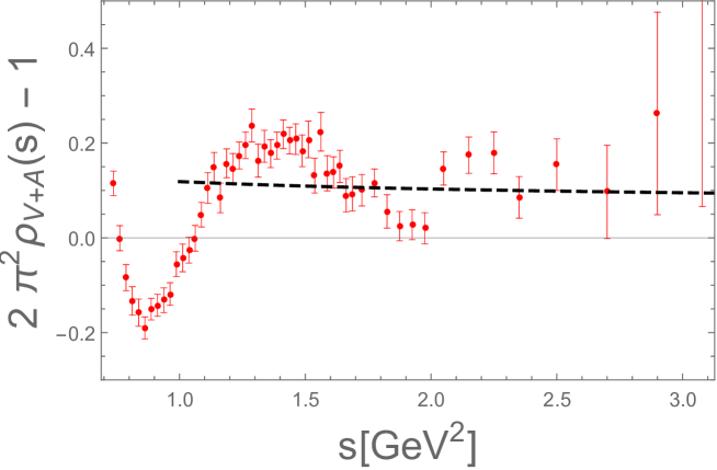
Figure 2: Blow-up of the ALEPH data (red data points) in the large-$s$ region of the $V+A$ non-strange spectral function ($s$ in GeV²). What is shown is $2\pi^{2}\rho_{V+A}-1$, i.e., the dynamical QCD contribution to the spectral distribution. Black dashed line: perturbation theory (CIPT) representation of the model, also with the parton-model contribution subtracted.

In Fig. 2 we show the large-$s$ region of the non-strange, $V+A$ spectral-function obtained from ALEPH data ALEPH13 . We have plotted $2\pi^{2}\rho_{V+A}-1$, rather than $2\pi^{2}\rho_{V+A}$, in order to remove the free-quark (or parton-model) contribution, which is independent of QCD dynamics; $2\pi^{2}\rho_{V+A}-1$ thus represents the dynamical QCD contribution to the spectral distribution. The difference between the dashed curve and the horizontal axis in Fig. 2 represents the perturbative part of the dynamics from which $\alpha_{s}$ is extracted. It is clear that DVs, represented by the oscillations of the data around the dashed curve, are not a small part of the dynamical QCD contribution to the spectral function in this region. This is especially evident in the region below $s=2.3$ GeV², where the data errors are small. In addition, there is no sign in this region of a strong damping of these oscillations. Therefore, even though above $s=2.3$ GeV² the errors are large enough for the data to be in rough agreement with the dashed curve, it is not safe to assume that DVs are small enough to be irrelevant in the region up to $s=m_{\tau}^{2}$.

We can study the effects of DVs quantitatively. As a first exercise, we consider how a quantitatively reasonable representation of the duality-violating part of the spectral function, $\rho_{V+A}^{\rm DV}(s)=\rho_{V}^{\rm DV}(s)+\rho_{A}^{\rm DV}(s)$, affects the results of the truncated-OPE strategy. We take our representation of DVs from one of the fits of Ref. alphas14 , and assume values for the OPE coefficients $C_{10}$ through $C_{16}$ which are consistent with FESRs that account for these DVs. From Ref. alphas14 , we take

$$\delta_{V} =3.35\ ,\qquad\qquad\delta_{A} =1.59\ ,$$ (17)

$$\gamma_{V} =0.70\ ,\qquad\qquad\gamma_{A} =1.44\ ,$$

$$\alpha_{V} =4.00\ ,\qquad\qquad\alpha_{A} =5.37\ ,$$

$$\beta_{V} =4.23\ ,\qquad\qquad\beta_{A} =2.03\ ,$$

(with $\gamma_{V,A}$ and $\beta_{V,A}$ in GeV^-2). In Sec. 7 of Ref. alphas14 we used the results of this fit to estimate the values for all OPE coefficients $C_{D}$, $D=4,\dots,16$. For the CIPT case, the estimates we need here are

$$C_{8} = 0.0349~{}\mbox{GeV}^{8}\ ,$$ (18)

$$C_{10} = -0.0832~{}\mbox{GeV}^{10}\ ,$$

$$C_{12} = 0.161~{}\mbox{GeV}^{12}\ ,$$

$$C_{14} = -0.191~{}\mbox{GeV}^{14}\ ,$$

$$C_{16} = -0.233~{}\mbox{GeV}^{16}\ .$$

For the exercise below, whose purpose is to illustrate the sensitivity of the output $\alpha_{s}$ to the input values assumed for the higher dimension $C_{D}$, it suffices to use these same values for the FOPT exploration as well.

Assuming the values given in Eq. (18) for $C_{8}$ through $C_{16}$, and keeping the second term on the right-hand side of Eq. (10), using the DV parameters of Eq. (17), we find the results shown in Tables 11, 12, 13 and 14 by applying the strategy of Ref. Pich using the weights in Eq. (12), the reduced weights (13), the “optimal” weights (14), or the weights (15).

	$\alpha_{s}(m_{\tau}^{2})$	$C_{4}$ (GeV4)	$C_{6}$ (GeV6)	$C_{8}$ (GeV8)	$\chi^{2}/$dof
FOPT	0.297(3)	0.0042(3)	-0.0126(3)	0.0353(3)	1.30/1
CIPT	0.310(4)	0.0029(4)	-0.0124(3)	0.0352(3)	1.00/1

Table 11: Fits as in Table 1, but with $C_{10}$, $C_{12}$, $C_{14}$ and $C_{16}$ as given in Eq. (18), and including the DV parameters of Eq. (17). Errors are statistical only.

	$\alpha_{s}(m_{\tau}^{2})$	$C_{4}$ (GeV4)	$C_{6}$ (GeV6)	$C_{8}$ (GeV8)	$\chi^{2}/$dof
FOPT	0.297(3)	0.0041(2)	-0.0126(2)	0.0352(2)	1.20/1
CIPT	0.310(3)	0.0028(2)	-0.0126(2)	0.0351(1)	0.90/1

Table 12: Fits as in Table 2, but with $C_{10}$, $C_{12}$ and $C_{14}$ as given in Eq. (18), and including the DV parameters of Eq. (17). Errors are statistical only.

	$\alpha_{s}(m_{\tau}^{2})$	$C_{6}$ (GeV6)	$C_{8}$ (GeV8)	$C_{10}$ (GeV10)	$\chi^{2}/$dof
FOPT	0.296(4)	-0.0127(4)	0.0354(5)	-0.0834(3)	1.36/1
CIPT	0.310(5)	-0.0128(4)	0.0353(5)	-0.0834(3)	1.06/1

Table 13: Fits as in Table 3, but with $C_{12}$, $C_{14}$ and $C_{16}$ as given in Eq. (18), and including the DV parameters of Eq. (17). Errors are statistical only.

	$\alpha_{s}(m_{\tau}^{2})$	$C_{4}$ (GeV4)	$C_{6}$ (GeV6)	$\chi^{2}/$dof
FOPT	0.301(9)	0.004(1)	-0.012(2)	2.04/1
CIPT	0.313(11)	0.003(1)	-0.012(2)	1.95/1

Table 14: Fits as in Table 4, but with $C_{8}$ as given in Eq. (18), and including the DV parameters of Eq. (17). Errors are statistical only.

Again, these fits are good fits, and they are consistent with each other. We note that the fits of Table 14 are more susceptible to DVs, because the weights (15) include polynomials which are less pinched than the weights of the other sets. We also note that including DVs changes the results of Table 10 into those shown in Table 14, which are in excellent agreement with the results in the other tables. The FOPT values for $\alpha_{s}(m_{\tau}^{2})$ are about 0.02 lower than those in Tables 1, 2, 3 and 4, while the CIPT values are about 0.025 lower. Perhaps not surprisingly, they are in good agreement with the values found in Ref. alphas14 . This suggests that the OPE can possibly be trusted at $s\approx-m_{\tau}^{2}$ up to $D=16$, even if it is an asymptotic expansion. However, it is also clear that solutions to the truncated-OPE fit strategy exist with OPE coefficients that cannot be considered small enough to be set equal to zero beyond $C_{8}$ (or $C_{10}$ for fits with “optimal” weights), and with DVs that cannot be neglected.

We also redid the “$A^{\omega^{(21)}}$” fits of Table 9 of Ref. Pich . What is done here is to take the moment with $w_{00}$ of Eq. (12) for values of $s_{0}$ ranging from $s_{0}=2.0$ GeV² to $s_{0}=m_{\tau}^{2}$, and fit these 9 data points as a function of $s_{0}$ to a fit function that includes $\alpha_{s}(m_{\tau}^{2})$, $C_{6}$ and $C_{8}$, ignoring DVs. We reproduced the values of Table 9 of Ref. Pich . Redoing these fits with DVs, we find values consistent with those of Tables 11 to 14, instead of Tables 1 to 4. Again, we conclude that the test of Table 9 of Ref. Pich does not provide a proof of the stability of the results, in contrast to what is suggested in Ref. Pich .

Finally, Ref. Pich introduces yet another set of weights that have an additional exponential suppression, similar in spirit to the moments employed in the SVZ sum rules of Ref. SVZ . Specifically, Ref. Pich considers a set of moments with weights $w_{B}(a,n)=(1-x^{n+1})e^{-ax}$, with $a\geq 0$. This type of moment acquires contributions from OPE condensates of all dimensions. In Ref. Pich , $\alpha_{s}$ was extracted from a single sum rule at a time, ignoring all non-perturbative corrections, for several values of $s_{0}$ and the Borel parameter $a$. We have reproduced their results and, in comparison to the plots of Ref. Pich , we find numerical agreement. The stability of the results regarding non-perturbative physics can be investigated by adding, successively, higher order terms in the OPE as well as adding or removing the DV contribution to the moments. For this exercise we employed the condensates of Eq. (18), as well as

$$C_{4} = 0.00268\ \mbox{GeV}^{4}\ ,$$ (19)

$$C_{6} = -0.0125\ \mbox{GeV}^{6}\ .$$

These values are again taken from Sec. 7 of Ref. alphas14 . The results thus obtained for $\alpha_{s}$ start stabilizing with respect to the OPE only after the term with $D=14$ is included. Together with the addition of the DV contribution, the results for $\alpha_{s}$ become then fully consistent with those of Tabs. 11, 12, 13 and 14. Values for $\alpha_{s}$ are systematically lower than in Ref. Pich and in good agreement with the ones found in Ref. alphas14 . In addition, the remaining instability with respect to the Borel parameter $a$ observed in Ref. Pich (for CIPT) is eliminated when the non-perturbative contributions are properly taken into account. We conclude that also this exploration does not validate the solution claimed by Ref. Pich .

In this section, we found that it is easy to find solutions to fits based on the truncated-OPE strategy yielding significantly different values for $\alpha_{s}(m_{\tau}^{2})$. Of course, at this point, none of these explorations tells us which solution is closest to the truth. Maybe none of them is; based on the exercises in this section, we cannot exclude the existence of yet other solutions to this collection of fits based on the truncated-OPE strategy. Even if the solution found in Ref. Pich would be the correct one, our results imply that it is impossible to assign a reliable systematic error to the values found for $\alpha_{s}(m_{\tau}^{2})$ based on the truncated-OPE-model strategy.

However, a very different type of test can be performed, in which we consider data constructed from a model compatible with the experimental V+A spectral function and having a known value for $\alpha_{s}(m_{\tau}^{2})$ and known DV contributions. The question then becomes whether the truncated-OPE strategy, applied to data constructed using this model, is able to successfully reproduce the known value of $\alpha_{s}(m_{\tau}^{2})$. We describe such a test in the next section.

IV A numerical experiment

In this section, we will carry out the “fake data” test. We start from a model of the $V+A$ spectral function which gives a good description of the real data from $s=1.55$ GeV² to $m_{\tau}^{2}$. The model value for the strong coupling is taken to be $\alpha_{s}(m_{\tau}^{2})=0.312$ (using CIPT), and the model has non-negligible DVs compatible with the real data; the corresponding parameters are given in Eq. (17). A multivariate Gaussian distribution is defined with model values at the ALEPH bin energies as central values, and with fluctuations around it controlled by the real-data covariance matrix ALEPH13 . This distribution is used to generate, probabilistically, a fake data set. To this fake data set we apply the truncated-OPE-model fits. We assess the reliability of the truncated-OPE-model by comparing the resulting fit values for $\alpha_{s}(m_{\tau}^{2})$ to the underlying true model value.

The key point is the following. Essentially, Ref. Pich claims that it is not necessary to take DVs explicitly into account, i.e., that they can be neglected for fits involving the (typically at least doubly-pinched) weights employed in previous implementations of the truncated-OPE strategy, cf. Sec. III. For the model, we know the value of $\alpha_{s}(m_{\tau}^{2})$ explicitly, and also know that it has significant DVs, by construction. It is also realistic, since it describes the spectral function data very well. Therefore, the truncated-OPE strategy, if reliable, should recover the model value of $\alpha_{s}(m_{\tau}^{2})$. If it does, the truncated-OPE strategy would pass this non-trivial test. If it does not, i.e., if it fails to recover the model value of $\alpha_{s}(m_{\tau}^{2})$ within statistical errors, the implication is that this strategy is incapable, in general, of finding the correct value from the real data with meaningful errors and is, thus, unreliable.

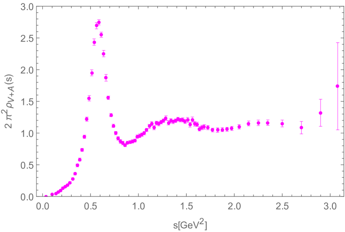
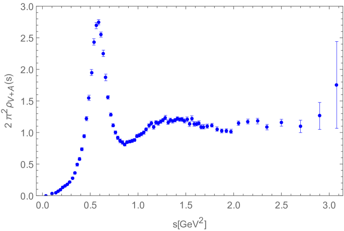
Figure 3: $V+A$ non-strange spectral function. Top panel: fake data, generated as described in the text, as a function of $s$. Bottom panel: true ALEPH data ALEPH13 as a function of $s$. The fake data have been generated for $s\geq 1.55$ GeV²; below this value the two data sets are the same.

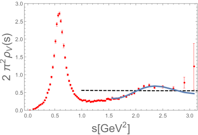
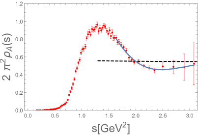
Figure 4: $V$ (left panel) and $A$ (right panel) non-strange spectral functions, as a function of $s$. Data points from Ref. ALEPH13 , curves represent the model described in the text for $s\geq 1.55\,\mathrm{GeV}^{2}$, and dashed lines show the perturbative part of the model.

IV.1 Fake data

We show the real data and the fake data in Fig. 3. These fake data have been generated by a model using CIPT for the perturbative part with $\alpha_{s}(m_{\tau}^{2})=0.312$. Correspondingly, we will carry out our test using CIPT. Note that the fake data resemble the real data strongly, and that, by construction, the covariance matrices for both data sets are identical. The DV parameters defining the duality-violating part of the fake data are given in Eq. (17). The ALEPH $V$ and $A$ spectral functions, together with the model representations using these DV parameters, are shown in Fig. 4. The model OPE coefficients follow from the exact FESR (7.3) in Ref. alphas14 , and have been given already in Eqs. (18) and (19).

IV.2 Test of the truncated-OPE-model strategy

We apply the truncated-OPE-model strategy directly to the fake data. Tables 15 to 18 employ the same fits used to produce Tables 1 to 4, except that now the real data have been replaced by the fake data. We show only CIPT fit results because the fake data have been generated from a model based on the CIPT perturbative scheme. This is, however, not essential; the same exercise can also be carried out for FOPT.

We see that the truncated-OPE strategy fails to reproduce the model value for $\alpha_{s}(m_{\tau}^{2})=0.312$ (by 5 to 7 $\sigma$ for Tables 15 to 17), even though the individual fits have good $\chi^{2}$ values, and results of the different fits look mutually consistent. The same is true of the results for the OPE coefficients, which come out much smaller in magnitude than the values given in Eqs. (18) and (19). In addition to this failure to reproduce the model parameter values, the results of this exercise also once more show that demonstrating internal consistency among the various fits of Ref. Pich does not allow one to conclude that the determination of $\alpha_{s}(m_{\tau}^{2})$ employing the truncated-OPE strategy is valid within its quoted errors. We have verified that the correct values of $\alpha_{s}(m_{\tau}^{2})$ and the OPE coefficients are reproduced, within statistical errors, if higher-dimension OPE coefficients and DVs are used as input for the fits, analogous to the tests in Tables 11 to 14. This exercise shows that not only does the truncated-OPE strategy not distinguish between significantly different solutions, but that, in general, its assumptions may end up driving it to a “solution” which is actually incorrect.

$\alpha_{s}(m_{\tau}^{2})$	$C_{4}$ (GeV4)	$C_{6}$ (GeV6)	$C_{8}$ (GeV8)	$\chi^{2}/$dof
0.334(4)	-0.0023(4)	0.0007(3)	-0.0008(4)	0.94/1

Table 15: CIPT fits employing the truncated-OPE strategy on the fake data, based on the weights of Eq. (12). By assumption, $C_{10}=C_{12}=C_{14}=C_{16}=0$. Errors are statistical only.

$\alpha_{s}(m_{\tau}^{2})$	$C_{4}$ (GeV4)	$C_{6}$ (GeV6)	$C_{8}$ (GeV8)	$\chi^{2}/$dof
0.334(3)	-0.0023(3)	0.0007(2)	-0.0007(2)	0.98/1

Table 16: CIPT fits employing the truncated-OPE strategy on the fake data, based on the reduced weights (13). By assumption, $C_{10}=C_{12}=C_{14}=0$. Errors are statistical only.

$\alpha_{s}(m_{\tau}^{2})$	$C_{6}$ (GeV6)	$C_{8}$ (GeV8)	$C_{10}$ (GeV10)	$\chi^{2}/$dof
0.334(4)	0.0008(4)	-0.0008(5)	0.0001(3)	0.92/1

Table 17: CIPT fits employing the truncated-OPE strategy on the fake data, based on the “optimal” weights (14) with $m=1$ and $n=1,\dots\,5$. By assumption, $C_{12}=C_{14}=C_{16}=0$. Errors are statistical only.

$\alpha_{s}(m_{\tau}^{2})$	$C_{4}$ (GeV4)	$C_{6}$ (GeV6)	$\chi^{2}/$dof
0.337(11)	-0.003(2)	0.001(2)	1.25/1

Table 18: CIPT fits employing the truncated-OPE strategy on the fake data, based on the weights of Eq. (15) with $n=0,\dots\,3$. By assumption, $C_{8}=0$. Errors are statistical only.

IV.3 Discussion

It is instructive to ask why the truncated-OPE-model strategy fails to reproduce the model values of $\alpha_{s}(m_{\tau}^{2})$ and the OPE coefficients. As we have seen in Secs. III.2.1 and III.2.2, setting the high-dimension OPE coefficients and the DVs to zero affects significantly the value of $\alpha_{s}(m_{\tau}^{2})$ extracted from the fits. Here, since we have the explicit spectral function for the fake data in hand, we can analyze the effects of the known DVs underlying these data on the fit strategy. These DVs affect the extraction of $\alpha_{s}$ directly through the term on the right hand side of Eq. (10), and also indirectly through the non-zero values shown in Eqs. (18) and (19) of the OPE condensates, $C_{D}$, obtained through Eq. (7.3) of Ref. alphas14 .

Let us consider Fig. 5, which shows again a blow-up of the large-$s$ region of the $V+A$ spectral function. The red experimental points represent the ALEPH data, and the thick blue curve shows the model representation of the $V+A$ spectral function, which is the sum of the model representations of the $V$ and $A$ spectral functions shown in Fig. 4 and as the blue dot-dashed curves in Fig. 5. The black dashed curve shows the perturbative part of the V+A model representation.

There are several important observations to make about this figure. First, we note that the model is not excluded by the data, even if one can imagine other models that might do equally well. Second, let us reiterate that it is not correct to think of DVs in this region of the spectral function as a “small effect.” The parton model (i.e., QCD to zeroth order in $\alpha_{s}$) contribution is given by a horizontal line at $2\pi^{2}\rho_{V+A}=1$. As already emphasized in Sec. III.2.2, it is the difference between the actual spectral function and this parton model horizontal line that contains the dynamics of QCD, and the duality-violating oscillations are not small on this scale. Third, one notes that the blue curve shows a duality-violating oscillation that is quite large at $s_{0}=m_{\tau}^{2}$, larger, in fact, than at any other value of $s_{0}$ larger than 1.7 GeV². This can happen over a limited range of $s$ even though the individual $V$ and $A$ DVs are exponentially damped. Since the truncated-OPE strategy of Ref. Pich simply assumes DVs to be suppressed to a negligible level in its $s_{0}=m_{\tau}^{2}$ fits without being able to test this assumption for validity, the result is that it is unable to reproduce the model value for $\alpha_{s}(m_{\tau}^{2})$ correctly.

Figure 5: Blow-up of the large-$s$ region of the $V+A$ non-strange spectral function. Black dashed line: the perturbative (CIPT) representation of the model. Blue curve: full model representation, including DVs. Blue dot-dashed curves: separate $V$ and $A$ parts of the model spectral function, shown also in Fig. 4.

V Modeling duality violations

There are two lessons to be learned from the failure of the truncated-OPE-model approach. First, DVs cannot simply be ignored. The data do not exclude the possibility that they are significant enough that they have to be taken into account in any high-precision fit of the data, which is, by experimental necessity, limited to $s\leq m_{\tau}^{2}$. This means, in practice, that DVs have to be modeled in order to carefully assess their contribution to any quantity extracted from these data.

Of course, modeling DVs, using Eq. (11), does two things. First, it introduces a new assumption into the analysis — the assumption that the model is good enough that results obtained for $\alpha_{s}(m_{\tau}^{2})$ from $\tau$ decays are reliable. While clearly the model (11) does a good job representing the data, it is possible that it does not give an accurate representation of the $V$ and $A$ spectral functions for $s>m_{\tau}^{2}$, where it is needed in the sum rule (10), but where no data are available alphas1 . However, ignoring DVs altogether in any type of fit to the data amounts to setting $\rho_{V/A}^{\rm DV}(s)=0$ in Eq. (11). Clearly, this is nothing else than a different choice of model. Given the oscillations visible in the data, we believe the choice that ignores DVs, in fact, to be a very poor model. In any case, our analysis in Secs. III and IV demonstrates that the model in which DVs are ignored does not lead to reliable results, irrespective of the question of the reliability of introducing an explicit model for DVs.

Second, once one models DVs explicitly, one is able to avoid artificially truncating the OPE. Instead, one can use the $s_{0}$ dependence of the spectral integrals in the region where the theoretical representation composed of the OPE and the DV ansatz works, thus avoiding spectral integrals involving weights that probe very high orders in the OPE. This approach, the DV-model strategy, was developed in Ref. alphas1 and applied there, and in Ref. alphas2 , to the OPAL data OPAL , and in Ref. alphas14 to the revised ALEPH data ALEPH13 .

V.1 Summary of the DV-model strategy of Ref. alphas14

We will not review, in this article, the DV-model strategy employed in our analyses of the $\tau$-decay data, as it has been explained in great detail in Refs. alphas1 ; alphas2 ; alphas14 . As indicated above, a model of the form (11) was used to parametrize DVs separately in the $V$ and $A$ channels, and the analysis was restricted to FESRs involving weights that probe OPE coefficients only up to dimension eight. Note that we also avoided weights with a term linear in $x$, which probe $C_{4}$, because of potential problems with such moments already in perturbation theory alphas1 ; BBJ12 . We varied $s_{0}\in[s_{\rm min},m_{\tau}^{2}]$ with $1.4~{}$GeV${}^{2}\leq s_{\rm min}\leq 1.7~{}$GeV², checking for stability as a function of $s_{\rm min}$, and carrying out many self-consistency tests between a large number of fits.

One of the tests we carried out is to consider the $s_{0}$ dependence of our fitted representation in comparison with the data for the spectral integrals with moments (12). We show, in Fig. 6, the results based on our $s_{\rm min}=1.55$ GeV² CIPT fit in Table 5 of Ref. alphas14 . What is plotted in each figure is the $s_{0}$-dependence of the spectral integral at $s_{0}=m_{\tau}^{2}$ minus the spectral integral at $s_{0}$. The presence of strong correlations in the data and the fits makes it necessary to plot such differences if one wishes to appropriately appraise the level of agreement between theory and data.

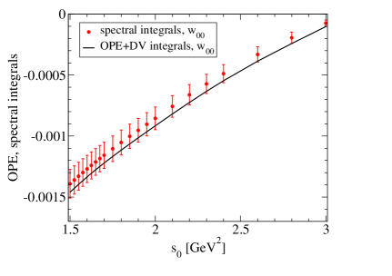
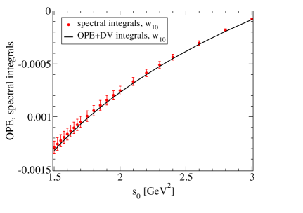
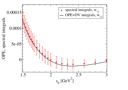
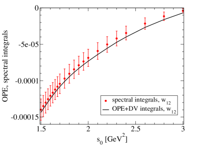
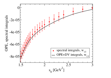
Figure 6: Comparison of $V+A$ spectral integrals with weights $w_{k\ell}$ of Eq. (12), using results of the CIPT fit with $s_{\rm min}=1.55$ GeV² of Table 5 of Ref. alphas14 with data, using the ALEPH data of Ref. ALEPH13 .

We note that, of the moments shown in Fig. 6, only $w_{00}$ was used explicitly in our fit. The OPE coefficients $C_{D}$, $D>8$, required to obtain the theoretical moments for the weights $w_{10}$, $w_{11}$, $w_{12}$ and $w_{13}$, were computed using the power weight $x^{N}$ FESRs at a single $s_{0}$ (chosen equal to $1.55$ GeV²) with our $\alpha_{s}$ and DV parameter fit results as input alphas14 . The resulting $C_{D}$ values are listed in Eq. (18). The agreement of the $w_{10}$, $w_{11}$, $w_{12}$ and $w_{13}$ spectral integrals with the corresponding theoretical representations, as a function of $s_{0}$, thus provides a test of the self-consistency of our strategy.

Figure 7 shows the same type of plots, but now using the results from the CIPT fit given in Table 1 (which corresponds to Table 1 of Ref. Pich ), obtained ignoring DVs, and setting $C_{10}=C_{12}=C_{14}=C_{16}=0$.

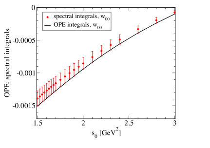
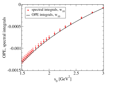
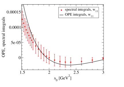
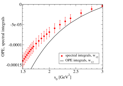
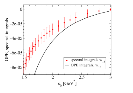
Figure 7: Comparison of $V+A$ spectral integrals with weights $w_{k\ell}$ of Eq. (12), using results of the CIPT fit in Table 1, i.e., Table 1 of Ref. Pich with data, using the ALEPH data of Ref. ALEPH13 .

Note that in this case all spectral integrals at $s_{0}=m_{\tau}^{2}$ were included in the fit. One clearly sees that the $s_{0}$ dependence deteriorates for weights which probe the higher-dimension terms in the OPE. The comparison of Figs. 6 and 7 clearly favors the DV-model strategy over the truncated-OPE strategy.

We have also considered examples of FOPT fits, again using our fit for $s_{\rm min}=1.55$ GeV² from Table 5 of Ref. alphas14 and the fit of Table 1 of Ref. Pich . We show the spectral integrals with weights $w_{10}$ and $w_{13}$ in Fig. 8. The two weights we chose to show are representative of the whole set, except for $w_{00}$ for which the DV-model-strategy plot looks as good as in the CIPT case. This is no surprise, as the $s_{0}$ dependence of the spectral integral with weight $w_{00}$ was used in the fits based on this strategy.

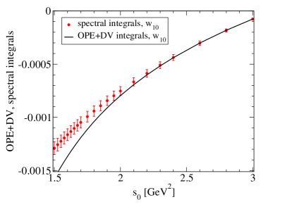
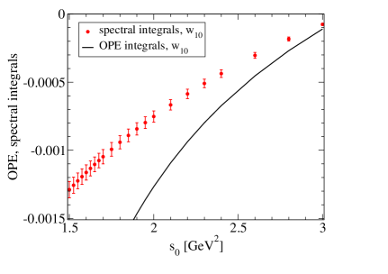
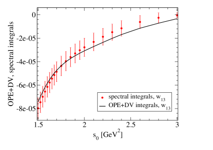
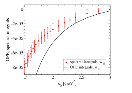
Figure 8: Comparison of $V+A$ spectral integrals with weights $w_{k\ell}$ of Eq. (12), using results of the FOPT fit with $s_{\rm min}=1.55$ GeV² of Table 5 of Ref. alphas14 (left panels), and using results of the FOPT fit in Table 1, i.e., Table 1 of Ref. Pich (right panels), with data, using the ALEPH data of Ref. ALEPH13 .

Although the performance of the DV model in the FOPT case is somewhat worse than in the CIPT case, it is still much better than that of the truncated-OPE model. We note that the results for $\alpha_{s}(m_{\tau}^{2})$ obtained with the DV-model strategy in Ref. alphas14 do not rely on spectral integrals with weights $w_{1\ell}$, whereas all these weights are used in the truncated-OPE strategy.

V.2 The criticism of Ref. Pich

In the preceding sections, we have demonstrated that the truncated-OPE-model strategy suffers from systematic problems which preclude its use as a method for obtaining a reliable determination of $\alpha_{s}(m_{\tau}^{2})$ from hadronic $\tau$ decays. It is, however, also relevant to ask whether the DV-model strategy provides an acceptable alternative, and Ref. Pich devoted a section to criticism of this strategy. The key criticisms raised by Ref. Pich are encapsulated in Fig. 6 and Table 10 of Ref. Pich . Here we will address these criticisms, both refuting them and at the same time commenting more specifically on some of their more misleading aspects.

First, we consider the argument based on Fig. 6 of Ref. Pich , which chooses to focus on the simplest, but non-central, fit of Ref. alphas14 . We reproduce this figure in Fig. 9. The fit considered in Ref. Pich is a fit of perturbation theory (FOPT) and the DV ansatz (11) to the $s_{0}$-dependent ($w=1$)-weighted integrals of the $V$ spectral function on the left-hand side of Eq. (10). The fit is performed in the interval $[s_{\rm min},m_{\tau}^{2}]$. Figure 9 shows the resulting $\alpha_{s}(m_{\tau}^{2})$ (left panel) and the $p$-value of the fit (right panel), as a function of $s_{\rm min}$. This figure is in good agreement with Fig. 6 of Ref. Pich . There are small differences; in particular, our $p$-values are somewhat higher, likely as a result of the somewhat more careful treatment of the ALEPH data in Ref. alphas14 (cf. footnote 6).

Let us now explain why the criticism of Ref. Pich based on these two plots is unjustified. With regard to the left panel of Fig. 9, Ref. Pich states that “the fitted values of $\alpha_{s}(m_{\tau}^{2})$ do not present the stability one would expect.” This is a misreading of the plot. By varying $s_{\rm min}$, as was also done in Ref. alphas14 , one lets the data decide whether a stability region exists. To the left of this region (if it exists), i.e., for smaller $s_{\rm min}$, the importance of non-perturbative effects not captured by perturbation theory or the DV ansatz (11) causes the value of $\alpha_{s}(m_{\tau}^{2})$ to move. For larger values of $s_{\rm min}$, there should be stability, but, as fewer points are included in the fit if $s_{\rm min}$ increases, the results will become noisier. This is precisely what one sees in Fig. 9, and there is, moreover, a nice “plateau” (region of stability) for $1.5$ GeV${}^{2}\,\raisebox{-1.72218pt}{\hbox to0.0pt{$\sim$\hss}}\raisebox{1.72218pt}{$<$}\,s_{\rm min}\,\raisebox{-1.72218pt}{\hbox to0.0pt{$\sim$\hss}}\raisebox{1.72218pt}{$<$}\,1.8$ GeV².

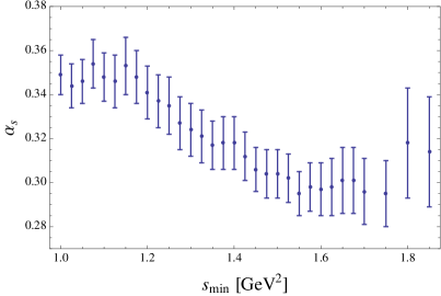
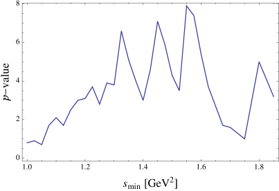
Figure 9: FOPT determination of $\alpha_{s}(m_{\tau}^{2})$ as a function of $s_{\rm min}$, using the $V$-channel $w=1$ fit of Ref. alphas14 .

With regard to the $p$-values shown in the right-hand panel, Ref. Pich states that “If the model were reliable, it should work better at higher hadronic invariant masses,” and takes both the size of the $p$-values in the region of the plateau, and the “significant deviations” at larger $s_{\rm min}$ as a signal of “poor statistical quality.” One should bear in mind, however, that the $p$-value of a fit is itself a statistical quantity, that will fluctuate with the data. For larger $s_{\rm min}$, the fluctuations in the data are more pronounced, and the $p$-values follow suit. Furthermore, a $p$-value of about 8% is generally not regarded as a proof of the failure of a hypothesis in a statistical analysis. In Ref. alphas14 many other fits where carried out (including multiple-weight V channel and combined V and A channel fits, and a combined $w=1$ $V$ and $A$ channel fit with $p$-values about double those of the corresponding $V$-channel-only fit. The results were also subjected to further tests, such as those provided by the Weinberg sum rules). The internal consistency of all these tests was taken as evidence for the likely validity of the final result.

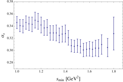
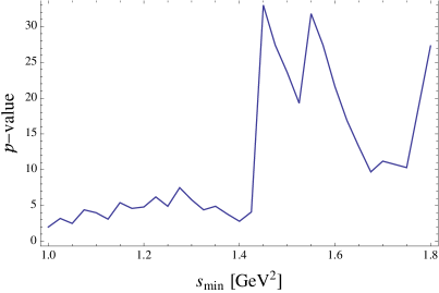
Figure 10: FOPT determination of $\alpha_{s}(m_{\tau}^{2})$ as a function of $s_{\rm min}$, using the $V$-channel $w=1$ fit of Ref. alphas14 , but now replacing the ALEPH data with fake data (see text).

We may further test this reasoning by repeating the DV-model analysis on a fake data set, as in Sec. IV. To do so, we generated a fake data set in the same way as in Sec. IV.1, but now for the $V$ channel only, using, to be specific, FOPT perturbation theory. The results of this exercise are shown in Fig. 10. The patterns are the same as those seen in Fig. 9. The only difference is that, in the case of Fig. 10, we know that the fake data has been constructed from a theoretical spectral function with $\alpha_{s}(m_{\tau}^{2})=0.297$ and the DV parameters given in the $s_{\rm min}=1.55$ GeV² FOPT line of Table IV in Ref. alphas14 .

Considering first the left panel of Fig. 10, we see that the pattern is consistent with the pattern seen in the left panel of Fig. 9. In addition, the fits find the correct values of $\alpha_{s}(m_{\tau}^{2})$ and the DV parameters $\delta_{V}$, $\gamma_{V}$, $\alpha_{V}$ and $\beta_{V}$ within errors. The stability plateau is located in the same $s_{\rm min}$ range in both figures. Also the right panels look very similar. For $s_{\rm min}\,\raisebox{-1.72218pt}{\hbox to0.0pt{$\sim$\hss}}\raisebox{1.72218pt}{$<$}\,1.4$ GeV², the fits to both the real and fake data have similar $p$-values, indicating that the theory representation works less well in that region, and stops working toward lower $s_{\rm min}$. For larger $s_{\rm min}$, the $p$-values of the fake-data fits are better than for the real-data fits. This is no surprise: after all, the theory is “perfect” for the fake data, whereas it is not expected to be so for the real data. More importantly, the large downward fluctuation near $s_{\rm min}=1.7$ GeV² is seen in both figures. By construction of the fake-data fits, the putative conclusion that these would be bad fits for the fake-data case is obviously incorrect. Therefore, the same conclusion cannot be drawn for the real-data fits either: it is not excluded that the feature seen around $s_{\rm min}=1.7$ GeV² in the right panel of Fig. 9 is nothing else than a fluctuation.

Turning now to the second point, let us briefly comment on Table 10 of Ref. Pich . Again, Ref. Pich considers the non-central, FOPT fit of the spectral integral with weight $w(x)=1$ of Ref. alphas14 . However, instead of using the DV ansatz as given in Eq. (11), it is now multiplied by $s^{n}$, with $n=0,\ 1,\ 2,\ 4,\ 8$ ($n=0$ corresponds to Eq. (11), of course). This makes very little sense, as follows from the discussion of the ansatz (11) at the end of Sec. II. While Eq. (11) introduces a particular model for DVs (which are a manifestation of the resonances one sees in the spectral functions), one should insist that any model incorporates what we know about the phenomenon the ansatz is supposed to model. In particular, Sec. II suggests that one might try to introduce a prefactor $1+a_{1}/s+a_{2}/s^{2}+\dots$, with new parameters $a_{1,2,\dots}$, reflecting the expectation that Eq. (11) emerges because of the suspected asymptotic nature of the OPE, for which the expansion parameter is $1/s$. The multiplication of Eq. (11) with an inverse power of this expansion parameter is, in view of these expectations, a wildly arbitrary choice, with no root in anything we know or suspect about the physics of QCD.

Despite the obvious shortcomings of the modifications to the DV ansatz employed in Ref. Pich , the fits shown in Table 10 of Ref. Pich , in fact, show a remarkable stability as a function of $n$. The $p$-values shown there are essentially constant. In terms of the criteria of Ref. Pich , where $1.5$ $\sigma$ central-value shifts are deemed indications of stability of the analysis, one would have to characterize the results for $\alpha_{s}(m_{\tau}^{2})$ as surprisingly constant: even the value at $n=8$, $\alpha_{s}(m_{\tau}^{2})=0.314(15)$, is just 1 $\sigma$ away from the central $n=0$ value $0.298$, while that at $n=4$ is closer to $0.5\sigma$ distant. The conclusion that such variations prove “model dependence,” as claimed in Ref. Pich , thus seems to us a somewhat surprising one. While we believe that the attempt of Ref. Pich to vary the DV model is theoretically unfounded and thus quite arbitrary, the tests of Table 10 in Ref. Pich in fact only serve to confirm the reliability of the results of Ref. alphas14 .

VI Conclusion

Our main goal in this article was a thorough investigation of the truncated-OPE-model strategy for extracting $\alpha_{s}(m_{\tau}^{2})$ from experimental data for hadronic $\tau$ decays. This strategy has been used extensively, notably in Refs. ALEPH13 ; Pich ; ALEPH ; OPAL . In a series of articles alphas1 ; alphas2 ; alphas14 we have designed and implemented a different strategy, the DV-model strategy. This strategy gives different results for $\alpha_{s}(m_{\tau}^{2})$, and it is thus important to understand and appraise the difference. In Refs. alphas1 ; alphas2 ; alphas14 we detailed the merits and assumptions of our strategy, and commented on the weaknesses of the truncated-OPE strategy as a motivation for the design of this alternate approach.

Reference Pich presented a detailed analysis of the determination of $\alpha_{s}$ based on the truncated-OPE strategy. This allowed us to devise a series of explicit tests to assess the validity of this approach; these are discussed in Secs. III and IV. These tests demonstrate unambiguously that the truncated-OPE strategy fails to produce reliable results for $\alpha_{s}(m_{\tau}^{2})$. In Sec. III we showed that varying the input values assumed for the higher dimension OPE condensates, $C_{D}$, in the truncated-OPE strategy can lead to significantly lower values for $\alpha_{s}(m_{\tau}^{2})$, about 8% lower in our example. This should be compared to the $<4\%$ total error claimed in Ref. Pich . In Sec. IV, we showed that the truncated-OPE strategy is incapable of detecting residual DVs, even when applied to a fake data set known to include them. As a consequence, it is incapable of reproducing the correct result for $\alpha_{s}$ in such a situation, finding instead a value about 7% too high in our fake-data test, and more than 5 $\sigma$ away from the true value on which the fake data is based. It is to be noted that 7-8% deviations are larger than the differences between the CIPT and FOPT values of the coupling. These failures result from shortcomings in the two main assumptions on which the truncated-OPE strategy is based: (1) the assumption that a number of higher-dimension OPE contributions can safely be set to zero by hand, for which there is no basis in QCD; (2) the assumption that DVs can be effectively neglected, even though the data clearly show resonance effects which, in the context of the FESR analysis, necessarily produce some level of quark-hadron duality violation. Our conclusion is that the truncated-OPE-model strategy does not hold up to detailed scrutiny, and should no longer be used for a precision determination of $\alpha_{s}(m_{\tau}^{2})$ from hadronic $\tau$ decays.

Of course, the alternative DV-model strategy should be subjected to similar scrutiny. Since this strategy was not the main topic of this article, we did not review the complete analysis of its application to the ALEPH data presented already in Ref. alphas14 , in which many consistency tests were carried out (our result for $\alpha_{s}(m_{\tau}^{2})$ is based on six different fits, and our analysis satisfies several $V-A$ sum rules within errors). Moreover, the fits reported in Tables 11 to 14 in Sec. III are fully consistent with the results of Ref. alphas14 , and thus provide further evidence for the stability of results obtained using the DV-model strategy. We also, in Sec. V.2, refuted the criticism of Ref. alphas14 contained in Sec. 7 of Ref. Pich , showing that the evidence on which this criticism was presumed to be based, in fact, actually provides further support for the validity of the DV-model strategy. In Sec. V.1 we contrasted the two strategies, showing how much better the DV-model strategy performs than the truncated-OPE strategy.

We are of course aware of the fact that the need to include a parametrization of DVs on the theory side of the FESR analysis of spectral functions obtained from hadronic $\tau$ decays leads to a certain model dependence in the strategy we employ. This is, however, true of both strategies: in the DV-model strategy, this is explicit, through the use of Eq. (11), while in the truncated-OPE-model strategy, it is implicit, through the neglect of DVs, which corresponds to the ansatz $\rho^{\rm DV}_{V/A}(s)=0$, $s\geq s_{0}$, and the uncontrolled truncation of the OPE. We reiterate that the investigation presented here shows unambiguously that the truncated-OPE-model fails to yield reliable results, and presents further evidence of the robustness of the DV-model approach. More precise data for the $V$ and $A$ spectral functions, possibly obtainable from $\tau$-decay data collected at BaBar and/or Belle, or from future $e^{+}e^{-}\to\mbox{hadrons}$ cross-section data, would make it possible to subject the DV-model strategy to more stringent tests than possible at present, using only OPAL and ALEPH data.

It has been pointed out that the results of Ref. alphas14 for $\alpha_{s}(m_{\tau}^{2})$, found using the revised ALEPH data ALEPH13 , lie about $0.03$ below those of Ref. alphas2 , found (using the same strategy) from the OPAL data OPAL . Assuming the two data sets to be uncorrelated, and largely because of the larger errors on the OPAL-based result, the difference amounts to about 1.4 $\sigma$. This means that the two determinations are consistent with each other, and thus that it is appropriate to consider their weighted average, as was done in Ref. alphas14 . This yields $\alpha_{s}(m_{\tau}^{2})=0.303(9)$ (FOPT) and $\alpha_{s}(m_{\tau}^{2})=0.319(12)$ (CIPT), results consistent with those of a recent, preliminary combined fit of the ALEPH and OPAL data reported in Ref. mainz .

In order to compare this result with that of the truncated-OPE-model strategy, we have to resort to the original OPAL analysis of the OPAL data OPAL , because Ref. Pich did not consider the OPAL data. In view of this, the best one can do is to combine the results of Ref. Pich , $\alpha_{s}(m_{\tau}^{2})=0.319(12)$ (FOPT) and $\alpha_{s}(m_{\tau}^{2})=0.335(13)$ (CIPT), with those of Ref. OPAL , $\alpha_{s}(m_{\tau}^{2})=0.324(15)$ (FOPT) and $\alpha_{s}(m_{\tau}^{2})=0.348(21)$ (CIPT). The weighted average between Ref. Pich and Ref. OPAL is $\alpha_{s}(m_{\tau}^{2})=0.321(9)$ (FOPT) and $\alpha_{s}(m_{\tau}^{2})=0.339(11)$ (CIPT). Again, these values, following from the truncated-OPE-model strategy, are about 0.02 larger than those following from the DV-model strategy, a difference comparable to that between the CIPT and FOPT determinations.

Without including OPAL data, the results from the two strategies are

$$\alpha_{s}(m_{\tau}^{2}) = 0.296(10)\qquad\mbox{(FOPT,\ DV-model strategy \cite[cite]{\@@bibref{Authors Phrase1YearPhrase2}{alphas14}{\@@citephrase{(}}{\@@citephrase{)}}})}\ ,$$ (20)

$$\alpha_{s}(m_{\tau}^{2}) = 0.310(14)\qquad\mbox{(CIPT,\ DV-model strategy \cite[cite]{\@@bibref{Authors Phrase1YearPhrase2}{alphas14}{\@@citephrase{(}}{\@@citephrase{)}}})}\ ,$$

$$\alpha_{s}(m_{\tau}^{2}) = 0.319(12)\qquad\mbox{(FOPT,\ truncated-OPE-model strategy \cite[cite]{\@@bibref{Authors Phrase1YearPhrase2}{Pich}{\@@citephrase{(}}{\@@citephrase{)}}})}\ ,$$ (21)

$$\alpha_{s}(m_{\tau}^{2}) = 0.335(13)\qquad\mbox{(CIPT,\ truncated-OPE-model strategy \cite[cite]{\@@bibref{Authors Phrase1YearPhrase2}{Pich}{\@@citephrase{(}}{\@@citephrase{)}}})}\ .$$

In this case, the difference between the results of the two strategies is about 0.024, larger than the roughly 0.015 difference between the individual CIPT and FOPT results. In this article, we have demonstrated that the values in Eq. (21) result from the use of a flawed fitting strategy, and provided further evidence for the reliability of the values in Eq. (20). The unreliable treatment of non-perturbative effects in the truncated-OPE-model strategy affects both the central value and uncertainties of $\alpha_{s}(m_{\tau}^{2})$. As such, we believe it is inappropriate to include values such as those in Eq. (21), obtained using this strategy, in any average for $\alpha_{s}(m_{\tau}^{2})$.

Acknowledgments

MG would like to thank Claude Bernard for discussions, the Instituto de Física de São Carlos of the Universidade de São Paulo for hospitality and FAPESP for partial support. This material is based upon work supported by the U.S. Department of Energy, Office of Science, Office of High Energy Physics, under Award Number DE-FG03-92ER40711. The work of DB is supported by the São Paulo Research Foundation (FAPESP) Grant No. 2015/20689-9 and by CNPq Grant No. 305431/2015-3. KM is supported by a grant from the Natural Sciences and Engineering Research Council of Canada. SP is supported by CICYTFEDER-FPA2014-55613-P, 2014-SGR-1450.

References

- (1)
- (2) M. Davier, A. Hoecker, B. Malaescu, C. Z. Yuan and Z. Zhang, Eur. Phys. J. C 74, 2803 (2014) [arXiv:1312.1501 [hep-ex]].
- (3) A. Pich and A. Rodríguez-Sánchez, Phys. Rev. D 94, no. 3, 034027 (2016) [arXiv:1605.06830 [hep-ph]].
- (4) D. Boito, O. Catà, M. Golterman, M. Jamin, K. Maltman, J. Osborne and S. Peris, Phys. Rev. D 84, 113006 (2011) [arXiv:1110.1127 [hep-ph]].
- (5) D. Boito, M. Golterman, M. Jamin, A. Mahdavi, K. Maltman, J. Osborne and S. Peris, Phys. Rev. D 85, 093015 (2012) [arXiv:1203.3146 [hep-ph]].
- (6) D. Boito, M. Golterman, K. Maltman, J. Osborne and S. Peris, Phys. Rev. D 91, 034003 (2015) [arXiv:1410.3528 [hep-ph]].
- (7) R. Shankar, Phys. Rev. D 15, 755 (1977); R. G. Moorhouse, M. R. Pennington and G. G. Ross, Nucl. Phys. B 124, 285 (1977); K. G. Chetyrkin and N. V. Krasnikov, Nucl. Phys. B 119, 174 (1977); K. G. Chetyrkin, N. V. Krasnikov and A. N. Tavkhelidze, Phys. Lett. B 76, 83 (1978); N. V. Krasnikov, A. A. Pivovarov and N. N. Tavkhelidze, Z. Phys. C 19, 301 (1983); E. G. Floratos, S. Narison and E. de Rafael, Nucl. Phys. B 155, 115 (1979); R. A. Bertlmann, G. Launer and E. de Rafael, Nucl. Phys. B 250, 61 (1985).
- (8) E. Braaten, Phys. Rev. Lett. 60, 1606 (1988).
- (9) E. Braaten, S. Narison, and A. Pich, Nucl. Phys. B 373 (1992) 581.
- (10) R. Barate et al. [ALEPH Collaboration], Eur. Phys. J. C 4, 409 (1998); S. Schael et al. [ALEPH Collaboration], Phys. Rept. 421, 191 (2005) [arXiv:hep-ex/0506072];
- (11) K. Ackerstaff et al. [OPAL Collaboration], Eur. Phys. J. C 7 (1999) 571 [arXiv:hep-ex/9808019].
- (12) P. A. Baikov, K. G. Chetyrkin and J. H. Kühn, Phys. Rev. Lett. 101 (2008) 012002 [arXiv:0801.1821 [hep-ph]].
- (13) A. A. Pivovarov, Z. Phys. C 53, 461 (1992) [Sov. J. Nucl. Phys. 54, 676 (1991)] [Yad. Fiz. 54 (1991) 1114] [arXiv:hep-ph/0302003]; F. Le Diberder and A. Pich, Phys. Lett. B 286, 147 (1992).
- (14) M. Jamin, JHEP 0509, 058 (2005) [hep-ph/0509001].
- (15) M. Beneke and M. Jamin, JHEP 0809, 044 (2008) [arXiv:0806.3156 [hep-ph]].
- (16) E. C. Poggio, H. R. Quinn, S. Weinberg, Phys. Rev. D 13, 1958 (1976).
- (17) O. Catà, M. Golterman, S. Peris, Phys. Rev. D 79, 053002 (2009) [arXiv:0812.2285 [hep-ph]].
- (18) O. Catà, M. Golterman, S. Peris, Phys. Rev. D 77, 093006 (2008) [arXiv:0803.0246 [hep-ph]].
- (19) O. Catà, M. Golterman, S. Peris, JHEP 0508, 076 (2005) [hep-ph/0506004].
- (20) B. Blok, M. A. Shifman and D. X. Zhang, Phys. Rev. D 57, 2691 (1998) [Erratum-ibid. D 59, 019901 (1999)] [arXiv:hep-ph/9709333]; I. I. Y. Bigi, M. A. Shifman, N. Uraltsev, A. I. Vainshtein, Phys. Rev. D 59, 054011 (1999) [hep-ph/9805241]; M. A. Shifman, [hep-ph/0009131]; M. Golterman, S. Peris, B. Phily, E. de Rafael, JHEP 0201, 024 (2002) [hep-ph/0112042].
- (21) M. Jamin, JHEP 1109, 141 (2011) [arXiv:1103.2718 [hep-ph]].
- (22) M. González-Alonso, A. Pich and A. Rodríguez-Sánchez, Phys. Rev. D 94, no. 1, 014017 (2016) [arXiv:1602.06112 [hep-ph]].
- (23) D. Boito, A. Francis, M. Golterman, R. Hudspith, R. Lewis, K. Maltman and S. Peris, Phys. Rev. D 92, no. 11, 114501 (2015) [arXiv:1503.03450 [hep-ph]].
- (24) M. Beneke, Phys. Rept. 317, 1 (1999) [hep-ph/9807443].
- (25) F. Le Diberder, A. Pich, Phys. Lett. B 289, 165 (1992).
- (26) K. Maltman, Phys. Lett. B 440, 367 (1998) [hep-ph/9901239].
- (27) C. A. Dominguez and K. Schilcher, Phys. Lett. B 448, 93 (1999) [hep-ph/9811261].
- (28) S. Peris, D. Boito, M. Golterman and K. Maltman, Mod. Phys. Lett. A 31 (2016) no.30, 1630031 [arXiv:1606.08898 [hep-ph]].
- (29) M. A. Shifman, A. I. Vainshtein and V. I. Zakharov, Nucl. Phys. B 147, 385 (1979).
- (30) M. Beneke, D. Boito and M. Jamin, JHEP 1301, 125 (2013) [arXiv:1210.8038 [hep-ph]].
- (31) D. Boito, M. Golterman, K. Maltman and S. Peris, Mod. Phys. Lett. A 31 (2016), no. 26, 1630024 [arXiv:1606.08899 [hep-ph]].