Geometric measures of quantum correlations with Bures and Hellinger distances

Abstract

This article contains a survey of the geometric approach to quantum correlations, to be published in the book “Lectures on General Quantum Correlations and their Applications” edited by F. Fanchini, D. Soares-Pinto, and G. Adesso (Springer, 2017). We focus mainly on the geometric measures of quantum correlations based on the Bures and quantum Hellinger distances.

1 Introduction

Quantum correlations in composite quantum systems are at the origin of the most peculiar features of quantum mechanics such as the violation of Bell’s inequalities and non-locality. In quantum information theory, they are viewed as quantum resources used by quantum algorithms and communication protocols to outperform their classical analogs. If the composite system is in a mixed state, classical correlations between the parties – arising e.g. from a random state preparation – may be present at the same time as quantum correlations. In two seminal papers, Ollivier and Zurek [66] and Henderson and Vedral [41] proposed a way to separate in bipartite systems classical from quantum correlations and introduced the quantum discord as a quantifier of the latter. For pure states, this quantifier coincides with the entanglement of formation, in agreement with the fact that quantum correlations  in pure states are synonymous to entanglement. For mixed states, however, the states with a vanishing discord, i.e. those states which possess only classical correlations, form a small (zero-measure) subset of the set of separable states. It has been argued that a non-zero discord could be responsible for the quantum speed-up of the DQC1 algorithm [26, 27]. Furthermore, the discord can be interpreted as the cost of quantum communication in certain protocols such as quantum state merging [56, 20, 60] and can be related to the distillable entanglement between one subsystem and a measurement  apparatus [86, 73]. On the other hand, the evaluation of the quantum discord remains a difficult challenge, even in the simplest case of two qubits (see [35, 60] and references therein).

In this chapter, we study alternative measures of quantum correlations  which share many of the properties of the quantum discord while being easier to compute and enabling for operational interpretations in terms of state distinguishability. Such measures are related to the geometry of the set of quantum states ${\cal E}({\cal H}_{AB})$ of the bipartite system ${AB}$. Actually, they are defined in terms of a distance on ${\cal E}({\cal H}_{AB})$. Apart from easier computability and operational interpretations, a notable advantage of the geometric approach is that it provides additional tools going beyond the quantification of correlations. In particular, one can determine the closest separable and closest classically-correlated states to a given state $\rho$, as well as the geodesics linking $\rho$ to those states. These tools may be useful when studying dissipative dynamical evolutions. For instance, one can gain some insight on the efficiency of a dynamical process in changing the amount of entanglement or quantum correlations by comparing the physical trajectory $t\mapsto\rho_{t}$ in ${\cal E}({\cal H}_{{AB}})$ with the geodesics connecting $\rho_{t}$ to its closest separable or classically-correlated state(s).

The aim of what follows is to introduce and review the main properties of a few geometric measures of quantum correlations depending on the choice of a distance on ${\cal E}({\cal H}_{AB})$. Instead of discussing the (huge amount of) different measures present in the literature, we shall restrict our attention to three quantities. We will mainly focus on (1) the geometric discord [25], defined as the minimal distance between the bipartite state $\rho$ and a classically-correlated state. We compare this discord with two other measures characterizing the sensitivity of the state to local measurements and unitary perturbations on one subsystem, namely (2) the measurement-induced geometric discord [55], defined as the minimal distance between $\rho$ and the corresponding post-measurement state after an arbitrary local measurement on subsystem $A$, and (3) the discord of response [32, 34], defined as the minimal distance between $\rho$ and its time-evolved version after an arbitrary local unitary evolution on $A$ implemented by a unitary operator with a fixed non-degenerate spectrum. As indicated in the title of the chapter, we will only consider two distinguished distances on the set of quantum states, namely the Bures and Hellinger distances. The discord of response for these two distances corresponds (in a sense that will become clear below) to well known measures of quantum correlations having clear operational interpretations, called the interferometric power [37] and Local Quantum Uncertainty (LQU) [36]. We will show that the geometric discord with Bures and Hellinger distances are related to a quantum state discrimination task, thereby establishing an explicit link between quantum correlations  and state distinguishability. We will also demonstrate that the geometric discord and discord of response with the Hellinger distance are almost as easy to compute as their analogs for the Hilbert-Schmidt distance (for instance, an explicit formula valid for arbitrary qubit-qudit states, which involves the coefficients of the expansion of the square root of the state in terms of generalized Pauli matrices, will be derived in Sec. 6.4). We point out that for the Bures and Hellinger distances, the measures (1)-(3) obey all the basic axioms of bona fide measures of quantum correlations, in contrast to what happens for the Hilbert-Schmidt distance [75]. Hence, the geometric discord and discord of response with the Hellinger distance offer the advantage of easy computability while being physically reliable.

The material of this chapter is to a large extend self-contained. The proofs of most results save for basic theorems related in textbooks (e.g. in Ref. [64]) are included. A few technical proofs are, however, omitted. We apologize to the authors of many papers related to geometric measures of quantum correlations  for not citing their works, either because they are not directly related to the results presented here or because we are not aware of them.

The remaining of the chapter is organized as follows. We recall in Sec. 2 the definitions of the entropic quantum discord and classically correlated states and formulate the basic postulates on measures of quantum correlations. The three measures outlined above are defined properly in Sec. 3. Sufficient conditions on the distance insuring that they obey the basic postulates are given in this section. A detailed review on the Bures and Hellinger distances and their metrics is provided in Sec. 4. Sections 5 and 6 are devoted to the geometric discord with the Bures and Hellinger distances, respectively. We present without proofs in Sec. 7 some results on the other two measures (2)-(3), in particular some bounds involving these measures and the geometric discord. The last section 8 contains a few concluding remarks.

2 Quantum vs classical correlations

2.1 Entropic quantum discord

In all what follows, we consider a bipartite quantum system ${AB}$, formed by putting together two systems $A$ and $B$, with Hilbert space ${\cal H}_{AB}={\cal H}_{A}\otimes{\cal H}_{B}$, ${\cal H}_{A}$ and ${\cal H}_{B}$ being the Hilbert spaces of the two subsystems. In the whole chapter, we only consider systems with finite dimensional Hilbert spaces, $n_{A}=\dim{\cal H}_{A}<\infty$ and $n_{B}=\dim{\cal H}_{B}<\infty$. Let us recall that a state of ${AB}$ is given by a density matrix $\rho$, that is, a non-negative operator on ${\cal H}_{AB}$ with unit trace $\operatorname{tr}\rho=1$. We write ${\cal E}({\cal H})$ the convex set formed by all density matrices on the Hilbert space ${\cal H}$. The extreme points of this convex set are the pure states $\rho_{\psi}=|\psi\rangle\langle\psi|$, with $|\psi\rangle\in{\cal H}$, $\|\psi\|=1$. We often abusively write $|\psi\rangle$ instead of $\rho_{\psi}$. Given a state $\rho\in{\cal E}({\cal H}_{AB})$ of the bipartite system ${AB}$, the reduced states of $A$ and $B$ are defined by partial tracing over the other subsystem, that is, $\rho_{A}=\operatorname{tr}_{B}(\rho)\in{\cal E}({\cal H}_{A})$ and $\rho_{B}=\operatorname{tr}_{A}(\rho)\in{\cal E}({\cal H}_{B})$. They correspond to the marginals of a joint probability in classical probability theory.

The quantum discord of Ollivier and Zurek [66] and Henderson and Vedral [41] is defined as follows. The total correlations between the two parties are characterized by the mutual information

$$I_{A:B}(\rho)=S(\rho_{B})+S(\rho_{A})-S(\rho)\;,$$ (1)

where the information (ignorance) about the state of ${AB}$ is given by the von Neumann entropy $S(\rho)=-\operatorname{tr}\rho\ln\rho$, and similarly for subsystems $A$ and $B$. In classical information theory, the mutual information is equal to the difference between the Shannon entropy of $B$ and the conditional entropy of $B$ conditioned on $A$. In the quantum setting, the corresponding difference is the Holevo quantity

$$\chi(\{\rho_{B|i},\eta_{i}\})=S(\rho_{B})-\sum_{i}\eta_{i}S(\rho_{B|i})\;,$$ (2)

where $\eta_{i}$ and $\rho_{B|i}$ are respectively the probability of outcome $i$ and the corresponding conditional state of $B$ after a local von Neumann measurement on $A$,

$$\eta_{i}=\operatorname{tr}\rho\,\Pi_{i}^{A}\otimes 1\quad,\quad\rho_{B|i}=\eta_{i}^{-1}\operatorname{tr}_{A}(\rho\,\Pi_{i}^{A}\otimes 1)\;.$$ (3)

Here, the measurement  is given by a family $\{\Pi_{i}^{A}\}$ of projectors satisfying $\Pi_{i}^{A}\Pi_{j}^{A}=\delta_{ij}\Pi_{i}^{A}$ and $\sum_{i}\Pi_{i}^{A}=1$ (hereafter, $1$ stands for the identity operator on ${\cal H}_{A}$, ${\cal H}_{B}$, or another space).

It turns out that, unlike in the classical case, $I_{A:B}(\rho)$ and $\chi(\{\rho_{B|i},\eta_{i}\})$ are not equal for general quantum states $\rho$, whatever the measurement  on $A$. One defines the quantum discord as the difference [66]

$$D_{A}^{\,\rm ent}(\rho)=I_{A:B}(\rho)-J_{B|A}(\rho)\quad,\quad J_{B|A}(\rho)=\max_{\{\Pi_{i}^{A}\}}\chi(\{\rho_{B|i},\eta_{i}\})\;,$$ (4)

where the maximum is over all projective measurements $\{\Pi_{i}^{A}\}$ on $A$. Alternatively, one can maximize over all POVMs $\{M_{i}^{A}\}$ on $A$ [41]. The quantum discord $D_{A}^{\rm\,ent}$ is interpreted as a quantifier of the non-classical correlations in the bipartite system. Note that it is not symmetric under the exchange of the two parties. One defines the discord $D_{B}^{\,\rm ent}$ analogously, by considering local measurements on subsystem $B$.

The two discords $D_{A}^{\,\rm ent}$ and $D_{B}^{\,\rm ent}$ give the amount of mutual information that cannot be retrieved by measurements on one of the subsystems. Actually, it is not difficult to show that:

Proposition 1.

[66] For any state $\rho\in{\cal E}({\cal H}_{AB})$,

$$D_{A}^{\,\rm ent}(\rho)=I_{A:B}(\rho)-\max_{\{\Pi^{A}_{i}\}}I_{A:B}\big{(}{\cal M}_{A}^{\Pi}\otimes 1(\rho)\big{)}\;,$$ (5)

where the maximum is over all projective measurements on $A$ with rank-one projectors $\Pi_{i}^{A}$ (or with rank-one operators $M_{i}^{A}$ if the maximization is taken over all POVMs in (4)) and

$${\cal M}_{A}^{\Pi}\otimes 1(\rho)=\sum_{i=1}^{n_{A}}\Pi_{i}^{A}\otimes 1\,\rho\,\Pi_{i}^{A}\otimes 1$$ (6)

is the post-measurement state in the absence of readout.

By using (5) and the contractivity of the mutual information under local quantum operations (data processing inequality), one finds that $D_{A}^{\,\rm ent}(\rho)\geq 0$ for any state $\rho$. Furthermore, $J_{B|A}(\rho)=I_{A:B}(\rho)-D_{A}^{\,\rm ent}(\rho)$ is equal to the maximum in the r.h.s.  of (5) and can thus be interpreted as the amount of classical correlations between the two parties (in fact, local measurements on $A$ remove all quantum correlations between $A$ and $B$). One can show that $J_{B|A}(\rho)=0$ if and only if  $\rho=\rho_{A}\otimes\rho_{B}$ is a product state.

It is not difficult to show that $D_{A}^{\,\rm ent}$ and $D_{B}^{\,\rm ent}$ coincide for pure states with the von Neumann entropy of the reduced states, i.e., with the entanglement of formation $E_{\rm EoF}$ [12, 13],

$$D_{A}^{\rm\,ent}(|\Psi\rangle)=D_{B}^{\rm\,ent}(|\Psi\rangle)=E_{\rm EoF}(|\Psi\rangle)=S([\rho_{\Psi}]_{A})=S([\rho_{\Psi}]_{B})\;.$$ (7)

In contrast, for mixed states $\rho$, $D_{A}^{\rm\,ent}(\rho)$ and $D_{B}^{\rm\,ent}(\rho)$ capture quantum correlations different from entanglement. In fact, mixed states can have a non-zero discord even if they are separable. Such states are obtained by preparing locally mixtures of non-orthogonal states, which cannot be perfectly discriminated by local measurements. An example of an $A$- and $B$-discordant two-qubit state with no entanglement is

$$\rho=\frac{1}{4}\bigl{(}|+\rangle\langle+|\otimes|0\rangle\langle 0|+|-\rangle\langle-|\otimes|1\rangle\langle 1|+|0\rangle\langle 0|\otimes|-\rangle\langle-|+|1\rangle\langle 1|\otimes|+\rangle\langle+|\bigr{)}$$ (8)

with $|\pm\rangle=(|0\rangle\pm|1\rangle)/\sqrt{2}$. The separable state (8) cannot be classified as “classical” and actually contains quantum correlations that are not detected by any entanglement measure.

It turns out that the evaluation of the discord $D_{A}^{\rm\,ent}(\rho)$ for mixed states $\rho$ is a challenging task, even for two-qubits [35, 60]. For the latter system, an analytical expression has been found so far for Bell-diagonal states only [54], while the formula proposed in [3] for the larger family of $X$-states happen to be only approximate [45, 60]. For a large number of qubits, the computation of the discord is an NP-complete problem [46].

2.2 Classical-quantum and classical states

States of a bipartite system ${AB}$ with a vanishing quantum discord with respect to $A$ possess only classical correlations. They are usually called classical-quantum states, but we shall prefer here the terminology “$A$-classical states”. One can show that a state $\sigma_{A\rm{-cl}}$ is $A$-classical if and only if  it is left unchanged by a local von Neumann measurement  on $A$ with rank-one projectors $\Pi_{i}^{A}$, i.e., $\sigma_{A\rm{-cl}}={\cal M}_{A}^{\Pi}\otimes 1(\sigma_{A\rm{-cl}})$, where ${\cal M}_{A}^{\Pi}$ is defined by (6). Therefore, all $A$-classical states are of the form

$$\sigma_{A\rm{-cl}}=\sum_{i=1}^{n_{A}}q_{i}|\alpha_{i}\rangle\langle\alpha_{i}|\otimes\rho_{B|i}\;,$$ (9)

where $\{|\alpha_{i}\rangle\}_{i=1}^{n_{A}}$ is an orthonormal basis of ${\cal H}_{A}$, $\{q_{i}\}$ is a probability distribution (i.e., $q_{i}\geq 0$ and $\sum_{i}q_{i}=1$), and $\rho_{B|i}$ are arbitrary states of $B$. Equation (9) means that the zero-discord states are mixtures of locally discernable states, that is, of states which can be perfectly discriminated by local measurements on $A$.

The $A$-classical states form a non-convex set ${\cal C}_{A}$, the convex hull of which is the set of all separable states ${\cal S}_{AB}$ of the bipartite system. It is clear from (9) that a pure state $|\Phi\rangle$ is $A$-classical if and only if  it is a product state $|\Phi\rangle=|\alpha\rangle|\beta\rangle$. Thus, for pure states classicality is equivalent to separability, as already evidenced by the relation (7). In contrast, most separable mixed states are not $A$-classical.

The $B$-classical states are defined analogously as the states with a vanishing discord with respect to subsystem $B$. They are of the form (9) with $\{|\alpha_{i}\rangle\}$ replaced by an orthonormal basis  $\{|\beta_{i}\rangle\}$ of ${\cal H}_{B}$ and $\rho_{B|i}$ by arbitrary states $\rho_{A|i}$ of $A$. The states which are both $A$- and $B$-classical are called classical states. They are of the form

$$\sigma_{\rm clas}=\sum_{i,j=1}^{n_{A},n_{B}}q_{ij}|\alpha_{i}\rangle\langle\alpha_{i}|\otimes|\beta_{j}\rangle\langle\beta_{j}|\;.$$ (10)

We denote by ${\cal C}_{B}$ and ${\cal C}_{AB}={\cal C}_{A}\cap{\cal C}_{B}$ the sets of $B$-classical states and of classical states, respectively. An illustrative picture of these subsets of the set of quantum states is displayed in Fig. 1. Note that this picture does not reflect all geometrical aspects (in particular, ${\cal C}_{A}$, ${\cal C}_{B}$, and ${\cal C}_{AB}$ typically have a lower dimensionality than ${\cal E}({\cal H}_{AB})$ and ${\cal S}_{AB}$).

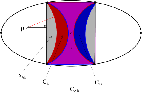
Figure 1: Schematic view of the set of quantum states ${\cal E}({\cal H}_{AB})$ of a bipartite system ${AB}$. The subset ${\cal C}_{AB}$ of classical states (in magenta) is the intersection of the subsets ${\cal C}_{A}$ and ${\cal C}_{B}$ of $A$- and $B$-classical states (in red and blue). The convex hull of ${\cal C}_{A}$ (or ${\cal C}_{B}$) is the subset ${\cal S}_{AB}$ of separable states (gray rectangle). All these subsets intersect the border of ${\cal E}({\cal H}_{AB})$ (which contains all pure states of ${AB}$) at the pure product states, represented by the four vertices of the rectangle. The maximally mixed state $\rho=1/(n_{A}n_{B})$ lies at the center (cross). The two points at the left and right extremities of the ellipse represent the maximally entangled pure states, which are the most distant states from ${\cal S}_{AB}$ (and also from ${\cal C}_{A}$, ${\cal C}_{B}$, and ${\cal C}_{AB}$). The square distances between a given state $\rho$ and ${\cal S}_{AB}$ (black line) and between $\rho$ and ${\cal C}_{A}$ (red line) define the geometric entanglement $E_{AB}^{\rm G}(\rho)$ and the geometric discord $D_{A}^{\rm G}(\rho)$, respectively.

2.3 Axioms on measures of quantum correlations

Before proceeding further, let us briefly recall the definition of a quantum operation (or quantum channel). We denote by ${\cal B}({\cal H})$ the $C^{\ast}$-algebra of bounded linear operators from ${\cal H}$ into itself, that is, $n\times n$ complex matrices with $\dim{\cal H}=n$ in our finite dimensional setting. Mathematically, a quantum operation  is a completely positive (CP) trace-preserving linear map ${\cal M}:{\cal B}({\cal H})\rightarrow{\cal B}({\cal H}^{\prime})$. Physically, quantum operations  represent either quantum evolutions or changes in the system state due to measurements  without readout like in (6). More precisely, let a quantum system ${S}$ initially in state $\rho_{S}$ be coupled at time $t=0$ to its environment ${E}$, with which it has never interacted at prior times. If the joint state $\rho_{SE}(t)$ of ${SE}$ either evolves unitarily according to the Schrödinger equation or is modified by a measurement process, then the reduced state of ${S}$ at time $t>0$ is given by $\rho_{S}(t)={\cal M}_{t}(\rho_{S})$ where ${\cal M}_{t}$ is a quantum operation.

By studying the properties of the quantum discord, one is led to define the following axioms for a bona fide measure of quantum correlations [36, 24, 37, 76, 83].

Definition 1.

A measure of quantum correlations on the bipartite system ${AB}$ is a non-negative function $D_{A}$ on the set of quantum states ${\cal E}({\cal H}_{AB})$ such that :

• $D_{A}(\rho)=0$ if and only if  $\rho$ is $A$-classical;

• $D_{A}$ is invariant under local unitary transformations, i.e., $D_{A}(U_{A}\otimes U_{B}\rho\,U_{A}^{\dagger}\otimes U_{B}^{\dagger})=D_{A}(\rho)$ for any unitaries $U_{A}$ and $U_{B}$ acting on ${\cal H}_{A}$ and ${\cal H}_{B}$;

• $D_{A}$ is monotonically non-increasing under quantum operations on $B$, i.e., $D_{A}(1\otimes{\cal M}_{B}(\rho))\leq D_{A}(\rho)$ for any quantum operation  ${\cal M}_{B}:{\cal B}({\cal H}_{B})\rightarrow{\cal B}({\cal H}_{B}^{\prime})$;

• $D_{A}$ reduces to an entanglement monotone on pure states.

These axioms are satisfied in particular by the entropic discord.

It can be shown that axioms (iii) and (iv) imply that, if the space dimensions of ${\cal H}_{A}$ and ${\cal H}_{B}$ are such that $n_{A}\leq n_{B}$, $D_{A}$ is maximum on maximally entangled pure states $|\Psi_{\rm me}\rangle$, i.e., if $\rho=\rho_{\Psi_{\rm me}}$ then $D_{A}(\rho)=D_{{\rm max}}$ [75]. It is argued in Ref. [78] that a proper measure of quantum correlations  $D_{A}$ must actually be such that the maximally entangled states are the only states satisfying $D_{A}(\rho)=D_{{\rm max}}$. We will thus consider the following additional axiom, fulfilled in particular by the entropic discord $D_{A}^{\,\rm ent}$ [83]:

• if $n_{A}\leq n_{B}$ then $D_{A}(\rho)$ is maximum if and only if $\rho$ is maximally entangled, that is, $\rho$ has maximal entanglement of formation $E_{\rm EoF}(\rho)=\ln n_{A}$.

Many authors have looked for functions $D_{A}\not=D^{\,\rm ent}_{A}$ on ${\cal E}({\cal H}_{AB})$ fulfilling axioms (i-iv), which can be used as $D^{\,\rm ent}_{A}$ to quantify quantum correlations in bipartite systems while being easier to compute and having operational interpretations. Among such measures, the distance-based measures studied in this chapter are especially appealing since they provide a geometric understanding of quantum correlations not limited to their quantification, as stressed in the Introduction.

3 Geometric measures of quantum correlations

3.1 Contractive distances on the set of quantum states

A fundamental issue in quantum information theory is the problem of distinguishing quantum states, that is, quantifying how “different” or how “far from each other” are two given states $\rho$ and $\sigma$. A natural way to deal with this problem is to endow the set of quantum states ${\cal E}({\cal H})$ with a distance $d$. One has a priori the choice between many distances. The most common ones are the $L^{p}$-distances

$$d_{p}(\rho,\sigma)=\|\rho-\sigma\|_{p}=\bigl{[}\operatorname{tr}(|\rho-\sigma|^{p})\bigr{]}^{\frac{1}{p}}$$ (12)

with $p\geq 1$ (here $|X|$ denotes the non-negative operator $|X|=\sqrt{X^{\dagger}X}$).

In quantum information theory, it is important to consider distances $d$ having the following property: if two identical systems in states $\rho$ and $\sigma$ undergo the same quantum evolution or are subject to the same measurement described by a quantum operation ${\cal M}$, then the time-evolved or post-measurement states ${\cal M}(\rho)$ and ${\cal M}(\sigma)$ cannot be farther from each other than the initial states $\rho$ and $\sigma$. In other words, the two states are less distinguishable after the evolution or the measurement, because some information has been lost in the environment or in the measurement apparatus. Distances $d$ on the sets of quantum states satisfying this property are said to be contractive under quantum operations (or “contractive” for short). More precisely, $d$ is contractive if for any finite-dimensional Hilbert spaces ${\cal H}$ and ${\cal H}^{\prime}$, any quantum operation ${\cal M}:{\cal B}({\cal H})\rightarrow{\cal B}({\cal H}^{\prime})$, and any $\rho$, $\sigma\in{\cal E}({\cal H})$, it holds

$$d({\cal M}(\rho),{\cal M}(\sigma))\leq d(\rho,\sigma)\;.$$ (13)

Note that a contractive distance is in particular unitary invariant, i.e.,

$$d\bigl{(}U\rho\,U^{\dagger},U\sigma\,U^{\dagger}\bigr{)}=d(\rho,\sigma)\quad\text{if $U$ is unitary on ${\cal H}$}$$ (14)

(in fact, $\rho\mapsto U\rho\,U^{\dagger}$ is an invertible quantum operation  on ${\cal B}({\cal H})$).

The relative von Neumann entropy $S(\rho||\sigma)=\operatorname{tr}[\rho(\ln\rho-\ln\sigma)]$ is a prominent example of contractive function on ${\cal E}({\cal H})\times{\cal E}({\cal H})$ and has a fundamental interpretation in terms of information. However, $S(\rho||\sigma)$ is not a distance (it is not symmetric under the exchange of $\rho$ and $\sigma$). It is desirable to work with contractive functions $d$ on ${\cal E}({\cal H})\times{\cal E}({\cal H})$ which can be interpreted like $S$ in terms of information while being true distances. It turns out that the $L^{p}$-distances $d_{p}$ are not contractive, with the notable exception of the trace distance $d_{1}$ [79, 67, 69]. Hence $d_{p}$, $p>1$ (and in particular the Hilbert-Schmidt distance $d_{2}$) cannot be reliably used to distinguish quantum states. We will focus in what follows on two particular distances, called the Bures and Hellinger distances, defined by

$$d_{\rm Bu}(\rho,\sigma) = \bigl{(}2-2\sqrt{F(\rho,\sigma)}\bigr{)}^{\frac{1}{2}}$$ (15)

$$d_{{\rm He}}(\rho,\sigma) = \big{(}2-2\operatorname{tr}\sqrt{\rho}\sqrt{\sigma}\big{)}^{\frac{1}{2}}\;,$$ (16)

where the Uhlmann fidelity is given by

$$F(\rho,\sigma)=\|\sqrt{\rho}\sqrt{\sigma}\|_{1}^{2}=\Bigl{(}\operatorname{tr}\bigl{[}(\sqrt{\sigma}\rho\sqrt{\sigma})^{\frac{1}{2}}\bigr{]}\Bigr{)}^{2}\;.$$ (17)

These distances will be studied in Sec. 4. We will show that they are contractive, enjoy a number of other nice properties, and are related to the Rényi relative entropies.

3.2 Distances to separable, classical-quantum, and product states

From a geometrical viewpoint, it is quite natural to quantify the amount of quantum correlations in a state $\rho$ of a bipartite system ${AB}$ by the distance $d(\rho,{\cal C}_{A})$ of $\rho$ to the subset ${\cal C}_{A}$ of $A$-classical states, i.e., by the minimal distance between $\rho$ and an arbitrary $A$-classical state (see Fig 1). This idea goes back to Vedral and Plenio [94, 95], who proposed to define the entanglement in ${AB}$ by the (square) distance from $\rho$ to the set of separable states ${\cal S}_{AB}$,

$$E^{\rm G}_{AB}(\rho)=d(\rho,{\cal S}_{AB})^{2}=\min_{\sigma_{\rm sep}\in{\cal S}_{AB}}d(\rho,\sigma_{\rm sep})^{2}\;.$$ (18)

These authors have shown that $E^{\rm G}_{AB}$ is an entanglement monotone if the distance $d$ is contractive. By analogy, Dakić, Vedral, and Brukner [25] introduced the geometric discord

$$D_{A}^{\rm G}(\rho)=d(\rho,{\cal C}_{A})^{2}=\min_{\sigma_{A\rm{-cl}}\in{\cal C}_{A}}d(\rho,\sigma_{A\rm{-cl}})^{2}\;.$$ (19)

Unfortunately, the distance $d$ was chosen in Ref. [25] to be the Hilbert-Schmidt distance $d_{2}$, which is not a good choice because $d_{2}$ is not contractive (Sec. 3.1). Further works have studied the geometric discords based on the more physically reliable Bures distance (see [2, 87, 81, 82, 1]), Hellinger distance (see [57, 78]), and trace distance (see [63, 68, 24] and references therein).

The discord $D^{\rm G}_{B}$ relative to subsystem $B$ is defined by replacing ${\cal C}_{A}$ by ${\cal C}_{B}$ in (19). Like for the entropic discord, one has in general $D_{A}^{\rm G}\not=D_{B}^{\rm G}$. Symmetric measures of quantum correlations are obtained by considering the square distance $D_{AB}^{\rm G}(\rho)=d(\rho,{\cal C}_{AB})^{2}$ to the set of classical states ${\cal C}_{AB}={\cal C}_{A}\cap{\cal C}_{B}$.

We emphasize that since ${\cal C}_{AB}\subset{\cal C}_{A}\subset{\cal S}_{AB}$ (see Fig. 1), the geometric measures are ordered as

$$E^{\rm G}_{AB}(\rho)\leq D_{A}^{\rm G}(\rho)\leq D_{AB}^{\rm G}(\rho)\;.$$ (20)

This ordering is a nice feature of the geometrical approach. In contrast, depending on $\rho$, the entanglement of formation $E_{\rm EoF}(\rho)$ can be larger or smaller than the entropic discord $D_{A}^{\rm ent}(\rho)$.

It is easy to show that $E_{AB}^{\rm G}$ is an entanglement monotone if the distance $d$ is contractive (this follows from the invariance of ${\cal S}_{AB}$ under LOCC operations, see [95, 83]) and that $E^{\rm G}_{AB}(\rho)=0$ if and only if  $\rho$ is separable (since a distance $d$ separates points). Hence $E^{\rm G}_{AB}$ qualifies as a reliable measure of entanglement. Similarly, one may ask whether the geometric discord $D_{A}^{\rm G}$ satisfies axioms (i-iv) of Definition 1. If $d$ is contractive, one easily shows that $D_{A}^{\rm G}$ obeys the first three axioms (i-iii). Finding general conditions on $d$ insuring the validity of the last axiom (iv) is still an open question. We will show below that (see Sec. 5.1, 5.2, and 6.1)

Proposition 2.

$D_{A}^{\rm G}$ is a bona fide measure of quantum correlations  when $d$ is the Bures or the Hellinger distance. Furthermore, if $d=d_{\rm Bu}$ then $D_{A}^{\rm G}$ satisfies the additional axiom (v).

It can be proven that $D_{A}^{\rm G}$ obeys axiom (v) also for the Hellinger distance $d_{\rm He}$ when $A$ is a qubit or a qutrit ($n_{A}=2$ or $n_{A}=3$) [78], and we believe that this is still true for higher dimensional spaces ${\cal H}_{A}$. It is conjectured by several authors that $D^{\rm G}_{A}$ is a bona fide measure of quantum correlations for the trace distance $d=d_{1}$, but as far as we are aware the justification of axiom (iv) is still open (however, this axiom holds for $n_{A}=2$, see e.g. [78]). In contrast, $D_{A}^{\rm G}$ is not a measure of quantum correlations  for the Hilbert-Schmidt distance $d=d_{2}$. Indeed, as one might expect from the fact that $d_{2}$ is not contractive, $D_{A}^{\rm G}$ does not fulfill axiom (iii) (an explicit counter-example is given in Ref. [74]).

One can replace the square distance by the relative entropy $S$ in formulas (18)-(19). Since $S$ is contractive under quantum operations  and satisfies $S(\rho||\sigma)=0$ if and only if  $\rho=\sigma$, one shows in the same way as for contractive distances that the corresponding entanglement measure $E^{\rm S}_{AB}$ is entanglement monotone [94] and that the discord $D_{A}^{\rm S}$ obeys axioms (i-iii). Furthermore, one finds that the closest separable state to a pure state $|\Psi\rangle$ for the relative entropy is a classical state and that $E^{\rm S}_{AB}(|\Psi\rangle)$ is equal to the entanglement of formation $E_{\rm EoF}(|\Psi\rangle)$ [95]. Hence $D_{A}^{\rm S}(|\Psi\rangle)=E^{\rm S}_{AB}(|\Psi\rangle)=E_{\rm EoF}(|\Psi\rangle)$ for any pure state $|\Psi\rangle\in{\cal H}_{AB}$. As a result, $D_{A}^{\rm S}$ is a bona fide measure of quantum correlations.

The mutual information (1) quantifying the total amount of correlations between $A$ and $B$ is equal to

$$I_{A:B}(\rho)=\min_{\sigma_{\rm prod}\in{\cal P}_{AB}}S(\rho||\sigma_{\rm prod})\;,$$ (21)

where ${\cal P}_{AB}=\{\sigma_{A}\otimes\sigma_{B};\sigma_{S}\in{\cal E}({\cal H}_{S}),S=A,B\}$ is the set of product (i.e., uncorrelated) states. In analogy with (21), one can define a geometrical mutual information $I_{AB}^{\rm G}$ and a measure $C_{A}^{\rm G}$ of classical correlations by [59, 18]

$$I_{AB}^{\rm G}(\rho)=d(\rho,{\cal P}_{AB})^{2}\quad,\quad C_{A}^{\rm G}(\rho)=\;\min_{\sigma_{\rho}\in{\cal C}_{A}}d(\sigma_{\rho},{\cal P}_{AB})^{2}\;,$$ (22)

where the minimum is over all closest $A$-classical states $\sigma_{\rho}$ to $\rho$. Unlike in the case of the entropic discord, the total correlations $I_{AB}^{\rm G}(\rho)$ is not the sum of the quantum and classical correlations $D_{A}^{\rm G}(\rho)$ and $C_{A}^{\rm G}(\rho)$ [59]. However, the triangle inequality yields $I_{AB}^{\rm G}(\rho)\leq(\sqrt{D_{A}^{\rm G}(\rho)}+\sqrt{C_{A}^{\rm G}(\rho)})^{2}$.

3.3 Response to local measurements and unitary perturbations

An alternative way to quantify quantum correlations  with the help of a distance $d$ is to consider the sensitivity of the state $\rho\in{\cal E}({\cal H}_{AB})$ to local measurements or local unitary perturbations.

• The distinguishability of $\rho$ with the corresponding post-measurement state after a local projective measurement on subsystem $A$ is characterized by the measurement-induced geometric discord, defined by [55]

  $$D_{A}^{\rm M}(\rho)=\min_{\{\Pi_{i}^{A}\}}d\bigl{(}\rho,{\cal M}^{\Pi}_{A}\otimes 1(\rho)\bigr{)}^{2}\;,$$ (23)

  where the minimum is over all measurements on $A$ with rank-one projectors $\Pi_{i}^{A}$ and ${\cal M}^{\Pi}_{A}$ is the associated quantum operation  (6). Since the outputs of such measurements are always $A$-classical, one has $D^{\rm G}_{A}(\rho)\leq D^{\rm M}_{A}(\rho)$ for any state $\rho$. This inequality is an equality if $d=d_{2}$ is the Hilbert-Schmidt distance [55]. For the Bures and Hellinger distances, $D_{A}^{\rm G}$ and $D_{A}^{\rm M}$ are in general different, even if $A$ is a qubit [78]. For the trace distance, $D_{A}^{\rm G}=D_{A}^{\rm M}$ when $A$ is a qubit but this is no longer true for $n_{A}>2$ [63].

• The distinguishability of $\rho$ with the corresponding state after a local unitary evolution on subsystem $A$ is characterized by the discord of response [32, 34, 76]

  $$D_{A}^{\rm R}(\rho)=\frac{1}{{\cal N}}\min_{U_{A},{\rm{sp}}(U_{A})=e^{{\rm{i}}\Lambda}}d\bigl{(}\rho,U_{A}\otimes 1\,\rho\,U_{A}^{\dagger}\otimes 1\bigr{)}^{2}\,,$$ (24)

  where the minimum is over all unitary operators $U_{A}$ on ${\cal H}_{A}$ separated from the identity by the condition of having a fixed spectrum ${\rm{sp}}(U_{A})=e^{{\rm{i}}\Lambda}=\{e^{2{\rm{i}}\pi j/n_{A}};j=0,\ldots,n_{A}-1\}$ given by the roots of unity. The normalization factor ${\cal N}$ in (24) depends on the distance and is chosen such that $D_{A}^{\rm R}(\rho)$ has maximal value equal to unity. For instance, ${\cal N}=2$ for the Bures, Hellinger, and Hilbert-Schmidt distances and ${\cal N}=4$ for the trace distance [78].

The measurement-induced geometric discord  and discord of response are special instances of measures of quantumness given by

$$Q_{\delta,{\cal F}_{A}}(\rho)=\inf_{{\cal M}_{A}\in{\cal F}_{A}}\delta(\rho,{\cal M}_{A}\otimes 1(\rho))\;,$$ (25)

where ${\cal F}_{A}$ is a family of quantum operations  on $A$ and $\delta$ is a (square) distance or a relative entropy. The following result of Piani, Narasimhachar, and Calsamiglia [75] is useful to check that such measures are bona fide measures of quantum correlations.

Theorem 1.

[75] For all spaces ${\cal H}$ with $\dim{\cal H}<\infty$, let $\delta(\rho,\sigma)$ be non-negative functions on ${\cal E}({\cal H})\times{\cal E}({\cal H})$ which are contractive under quantum operations  and satisfy the ‘flags’ condition

$$\delta\Big{(}\sum_{i}\eta_{i}\rho_{i}\otimes|i\rangle\langle i|,\sum_{i}\eta_{i}\sigma_{i}\otimes|i\rangle\langle i|\Big{)}=\sum_{i}\eta_{i}\delta(\rho_{i},\sigma_{i})\;,$$ (26)

where $\{|i\rangle\}$ is an orthonormal basis  of an ancilla Hilbert space ${\cal H}_{E}$. Assume that $n_{A}\leq n_{B}$. Let the family ${\cal F}_{A}$ of quantum operations  on ${\cal B}({\cal H}_{A})$ be closed under unitary conjugations. Then the measure of quantumness (25) satisfies axioms (ii-iv) of Definition 1.

Proof. We first show that $Q_{\delta,{\cal F}_{A}}$ is an entanglement monotone when restricted to pure states. It is known (see e.g. [64]) that when $n_{A}\leq n_{B}$, a LOCC acting on a pure state $|\Psi\rangle$ may always be simulated by a one-way communication protocol involving only three steps: (1) Bob first performs a measurement  with Kraus operators $\{B_{i}\}$ on subsystem $B$; (2) he sends his measurement  result to Alice; (3) Alice performs a unitary evolution $U_{i}$ on subsystem $A$ conditional to Bob’s result. Therefore, it is enough to show that for any pure state $|\Psi\rangle\in{\cal H}_{AB}$, any family $\{B_{i}\}$ of Kraus operators on ${\cal H}_{B}$ (satisfying $\sum_{i}B_{i}^{\dagger}B_{i}=1$), and any family $\{U_{i}\}$ of unitaries on ${\cal H}_{A}$, it holds

$$\sum_{i}\eta_{i}Q_{\delta,{\cal F}_{A}}(|\Phi_{i}\rangle)\leq Q_{\delta,{\cal F}_{A}}(|\Psi\rangle)\;,$$ (27)

where $\eta_{i}=\|1\otimes B_{i}|\Psi\rangle\|^{2}$ is the probability that Bob’s outcome is $i$ and $|\Phi_{i}\rangle=\eta_{i}^{-\frac{1}{2}}U_{i}\otimes B_{i}|\Psi\rangle$ is the corresponding conditional post-measurement  state after Alice’s unitary evolution. The inequality (27) is proven by considering the following quantum operation  ${\cal M}:{\cal B}({\cal H}_{AB})\rightarrow{\cal B}({\cal H}_{{AB}{E}})$

$${\cal M}(\rho)=\sum_{i}U_{i}\otimes B_{i}\,\rho\,U_{i}^{\dagger}\otimes B_{i}^{\dagger}\otimes|i\rangle\langle i|\;.$$ (28)

From the contractivity of $\delta$ and the flags condition, one gets

$$Q_{\delta,{\cal F}_{A}}(|\Psi\rangle) \geq \inf_{{\cal M}_{A}\in{\cal F}_{A}}\delta\bigl{(}{\cal M}(|\Psi\rangle\langle\Psi|)\,,\,{\cal M}\circ{\cal M}_{A}\otimes 1(|\Psi\rangle\langle\Psi|)\bigr{)}$$ (29)

$$= \inf_{{\cal M}_{A}\in{\cal F}_{A}}\delta\biggl{(}\sum_{i}\eta_{i}|\Phi_{i}\rangle\langle\Phi_{i}|\otimes|i\rangle\langle i|\,,\,\sum_{i}\eta_{i}{\cal M}_{A}^{(i)}\otimes 1(|\Phi_{i}\rangle\langle\Phi_{i}|)\otimes|i\rangle\langle i|\biggr{)}$$

$$= \inf_{{\cal M}_{A}\in{\cal F}_{A}}\sum_{i}\eta_{i}\,\delta\Bigl{(}|\Phi_{i}\rangle\langle\Phi_{i}|\,,\,{\cal M}_{A}^{(i)}\otimes 1(|\Phi_{i}\rangle\langle\Phi_{i}|)\Bigr{)}$$

with ${\cal M}_{A}^{(i)}(\cdot)=U_{i}{\cal M}_{A}(U_{i}^{\dagger}\cdot U_{i})U_{i}^{\dagger}$. Bounding the infimum of the sum by the sum of the infima and using the assumption $U_{i}{\cal F}_{A}U_{i}^{\dagger}={\cal F}_{A}$, one is led to the desired result

$$Q_{\delta,{\cal F}_{A}}(|\Psi\rangle)\geq\sum_{i}\eta_{i}\inf_{{\cal M}_{A}^{(i)}\in{\cal F}_{A}}\delta\Bigl{(}|\Phi_{i}\rangle\langle\Phi_{i}|,{\cal M}_{A}^{(i)}\otimes 1(|\Phi_{i}\rangle\langle\Phi_{i}|)\Bigr{)}=\sum_{i}\eta_{i}Q_{\delta,{\cal F}_{A}}(|\Phi_{i}\rangle)\;.$$ (30)

In particular, if the pure state $|\Psi\rangle$ can be transformed by a LOCC operation into the pure state $|\Phi\rangle$, which means that $|\Phi_{i}\rangle=|\Phi\rangle$ for all outcomes $i$, then $Q_{\delta,{\cal F}_{A}}(|\Psi\rangle)\geq Q_{\delta,{\cal F}_{A}}(|\Phi\rangle)$. Axiom (ii) follows from a similar argument and the unitary invariance of $\delta$ (which is a consequence of the contractivity assumption, see Sec. 3.1). Finally, one easily verifies that $Q_{\delta,{\cal F}_{A}}$ fulfills axiom (iii) by exploiting the contractivity of $\delta$. $\Box$

Proposition 3.

$D_{A}^{\rm M}$ and $D_{A}^{\rm R}$ are bona fide measures of quantum correlations  if the distance $d$ is contractive and $d^{2}$ satisfies the flag condition (24).

It is easy to show that the square Bures and Hellinger distances $d_{\rm Bu}^{2}$ and $d_{\rm He}^{2}$ satisfy the flags condition, so that Proposition 3 applies in particular to these distances. The result applies to the trace distance $d_{1}$ as well, see [75].

Proof. Let us first discuss axiom (i). For $D_{A}^{\rm M}$, its validity comes from the fact that a state is $A$-classical if and only if it is invariant under a von Neumann measurement on $A$ with rank-one projectors (Sec. 2.2). Note that this axiom would not hold if the minimization in (23) was performed over projectors $\Pi_{i}^{A}$ with ranks larger than one. For $D_{A}^{\rm R}$, one uses an equivalent characterization of $A$-classical states as the states $\rho$ which are left invariant by a local unitary transformation on $A$ for some unitary $U_{A}$ on ${\cal H}_{A}$ having a non-degenerate spectrum [76]. Actually, $U_{A}\otimes 1\rho U_{A}^{\dagger}\otimes 1=\rho$ if and only if  $\rho$ commutes with $U_{A}\otimes 1$, or, equivalently, with all its spectral projectors $\Pi_{i}^{A}$. This means that ${\cal M}_{A}^{\Pi}\otimes 1(\rho)=\rho$ with ${\cal M}_{A}^{\Pi}$ defined by (6). Since ${\rm{sp}}(U_{A})$ is not degenerate, the spectral projectors $\Pi_{i}^{A}$ have rank one. Consequently, the above condition on unitary transformations is equivalent to the invariance of $\rho$ under a measurement  on $A$ with rank-one projectors and thus to $\rho$ being $A$-classical. This proves that $D_{A}^{\rm R}$ satisfies axiom (i). The fact that $D_{A}^{\rm M}$ and $D_{A}^{\rm R}$ obey the other axioms (ii-iv) is a consequence of Theorem 1. $\Box$

As for the geometric discord, we do not have a general argument implying that $D_{A}^{\rm M}$ and $D_{A}^{\rm R}$ fulfill the additional axiom (v) under appropriate assumptions on the distance. However, one can show that $D^{\rm R}_{A}$ obeys axiom (v) for the Bures, Hellinger, and trace distances, and this is also true for $D^{\rm M}_{A}$ for the Bures distance [78].

3.4 Speed of response to local unitary perturbations

All distance-based measures of quantum correlations  defined above are global geometric quantities, in the sense that they depend on the distance between $\rho$ and states that are not in the neighborhood of $\rho$ (excepted of course when the measure vanishes). It is natural to look for quantifiers of quantum correlations  involving local geometric quantities depending only on the properties of ${\cal E}({\cal H}_{AB})$ in the vicinity of $\rho$. The idea of the sensitivity to local unitary perturbations sustaining the definition of the discord of response is well suited for this purpose. Indeed, instead of considering the minimal distance between $\rho$ and its perturbation by a local unitary with a fixed spectrum, one may consider the minimal speed at time $t=0$ of the time-evolved states

$$\rho_{\rm out}(t)=e^{-{\rm{i}}tH_{A}\otimes 1}\rho\,e^{{\rm{i}}tH_{A}\otimes 1}\;.$$ (31)

This leads to the definition of the discord of speed of response

$$D_{A}^{\rm SR}(\rho)=\min_{H_{A},{\rm{sp}}(H_{A})=\Lambda}\lim_{t\rightarrow 0}t^{-2}d\big{(}\rho,\rho_{\rm out}(t)\big{)}^{2}\;,$$ (32)

where the minimum is over all self-adjoint operators $H_{A}$ on ${\cal H}_{A}$ with a fixed non-degenerate spectrum $\Lambda=\{2\pi j/n_{A};j=0,\ldots,n_{A}-1\}$. This local geometric version of the discord of response has apparently not been defined before in the literature. The results of Propositions 4 and 5 below have up to our knowledge not been published elsewhere.

Proposition 4.

If the distance $d$ is contractive and Riemannian, and if $d^{2}$ satisfies the flags condition (26), then $D_{A}^{\rm SR}$ is a bona fide measure of quantum correlations. Furthermore, one has

$${\cal N}D_{A}^{\rm R}(\rho)\leq D_{A}^{\rm SR}(\rho)\;.$$ (33)

Proof. If $d$ is a Riemannian distance then the limit in (32) exists and is equal to $g_{\rho}(-i[H_{A}\otimes 1,\rho],-i[H_{A}\otimes 1,\rho])$ where $g$ is the metric associated to $d$ (see Sec. 4.6). Since $g_{\rho}$ is a scalar product, $D_{A}^{\rm SR}(\rho)=0$ if and only if  $[H_{A}\otimes 1,\rho]=0$ for some observable $H_{A}$ of $A$ with a non-degenerate spectrum ${\rm{sp}}(H_{A})=\Lambda$. As in the proof of Proposition 3, this is equivalent to $\rho$ being $A$-classical. Hence axiom (i) holds true. One easily convinces oneself that $D_{A}^{\rm SR}$ fulfills axioms (ii) and (iii) by using the unitary invariance and the contractivity of $d$, respectively. One deduces from the flags condition (26) for $\delta=d^{2}$ that the metric $g$ satisfies

$$g_{\rho_{{AB}{E}}}\bigg{(}\sum_{i}\eta_{i}\dot{\rho_{i}}\otimes|i\rangle\langle i|\,,\,\sum_{i}\eta_{i}\dot{\rho_{i}}\otimes|i\rangle\langle i|\bigg{)}=\sum_{i}\eta_{i}g_{\rho_{i}}(\dot{\rho_{i}},\dot{\rho_{i}})\quad\text{ for }\rho_{{AB}{E}}=\sum_{i}\eta_{i}\rho_{i}\otimes|i\rangle\langle i|\;.$$ (34)

Similarly, one infers from the contractivity of $d$ that the metric $g$ satisfies the inequality (66) below. By repeating the arguments in the proof of Theorem 1, one finds that $D_{A}^{\rm SR}$ is an entanglement monotone for pure states, i.e., it obeys axiom (iv).

The bound (33) is a consequence of the triangle inequality and the unitary invariance of $d$. Actually, one has

$$d\big{(}\rho,U_{A}\otimes 1\rho U_{A}^{\dagger}\otimes 1\big{)}^{2} \leq \lim_{N\rightarrow\infty}\biggl{\{}\sum_{n=1}^{N}d\Bigl{(}U_{A}^{\frac{n-1}{N}}\otimes 1\rho\big{(}U_{A}^{\frac{n-1}{N}}\big{)}^{\dagger}\otimes 1,U_{A}^{\frac{n}{N}}\otimes 1\rho(U_{A}^{\frac{n}{N}})^{\dagger}\otimes 1\Bigr{)}\biggr{\}}^{2}$$ (35)

$$= \lim_{N\rightarrow\infty}N^{2}d\Bigl{(}\rho,U_{A}^{\frac{1}{N}}\otimes 1\rho(U_{A}^{\frac{1}{N}})^{\dagger}\otimes 1\Bigr{)}^{2}=\lim_{t\rightarrow 0}t^{-2}d\big{(}\rho,\rho_{\rm out}(t)\big{)}^{2}\;,$$

where $\rho_{\rm out}(t)$ is given by (31) and $U_{A}=e^{{\rm{i}}H_{A}}$. $\Box$

Note that when subsystem $A$ is a qubit ($n_{A}=2$), the dependence of $D_{A}^{\rm SR}$ on the choice of the spectrum $\Lambda$ reduces to a multiplication factor. It follows from the physical interpretations of the Bures and Hellinger metrics (see Sec. 4.5 below) that

Proposition 5.

For invertible density matrices $\rho>0$, the discord of speed of response (32) coincides with

• the interferometric power [37] if $d=d_{\rm Bu}$ is the Bures distance:

  $$D_{A}^{\rm SR}(\rho)={\cal P}_{\Lambda}(\rho)=\frac{1}{4}\min_{H_{A},{\rm{sp}}(H_{A})=\Lambda}{\cal F}_{Q}(\rho,H_{A}\otimes 1)\;,$$ (36)

  where ${\cal F}_{Q}(\rho,H_{A}\otimes 1)$ is the quantum Fisher information giving the best precision in the estimation of the unknown parameter $t$ from arbitrary measurements on the output states (31).

• (twice the) Local Quantum Uncertainty (LQU) [36] if $d=d_{\rm He}$ is the Hellinger distance:

  $$D_{A}^{\rm SR}(\rho)=2LQU_{\Lambda}(\rho)=2\min_{H_{A},{\rm{sp}}(H_{A})=\Lambda}{\cal I}_{\rm skew}(\rho,H_{A}\otimes 1)\;,$$ (37)

  where ${\cal I}_{\rm skew}(\rho,H)=-\frac{1}{2}\operatorname{tr}([\sqrt{\rho},H]^{2})$ is the skew information [97] describing the amount of information on the values of observables not commuting with $H$ inferred from measurements on a system in state $\rho$.

This proposition shows that $D_{A}^{\rm SR}$ has operational interpretations related to parameter estimation and to quantum uncertainty in local measurements for the Bures and Hellinger distances, respectively.

If $n_{A}=2$ and $d=d_{\rm He}$ is the Hellinger distance, one finds that $D_{A}^{\rm R}$ and $D_{A}^{\rm SR}$ (i.e., the LQU) are proportional to each other,

$$LQU_{\{0,\pi\}}(\rho)=\frac{\pi^{2}}{4}D_{A}^{\rm R}(\rho)=\frac{\pi^{2}}{4}\inf_{\|{\vec{u}}\|=1}{\cal I}_{\rm skew}(\rho,\sigma_{\vec{u}}\otimes 1)$$ (38)

(this follows from the identity $2{\cal I}_{\rm skew}(\rho,U)=d_{\rm He}(\rho,U\rho U^{\dagger})^{2}$ for $U=U^{\dagger}=U^{-1}$ and from the aforementioned property of $D_{A}^{\rm SR}$ with respect to changes in the spectrum $\Lambda$).

3.5 Different quantum correlation measures lead to different orderings on ${\cal E}({\cal H})$

It may appear as an unpleasant fact that the orderings on the states of ${\cal E}({\cal H}_{AB})$ defined by the different measures of quantum correlations  are in general different, in particular they depend on the choice of the distance $d$. This means that, for instance, it is possible to find two states $\rho$ and $\sigma$ which satisfy $D^{\rm R}_{A}(\rho)<D^{\rm R}_{A}(\sigma)$ for the Bures distance and the reverse inequality $D^{\rm R}_{A}(\rho)>D^{\rm R}_{A}(\sigma)$ for the Hellinger distance. This is illustrated in Fig. 2. This figure displays the distributions in the planes defined by pairs of discords of response based on different distances for randomly generated two-qubit states $\rho$ with a fixed purity $P=\operatorname{tr}(\rho^{2})$ (a similar figure would be obtained if the purity was not fixed). The different orderings translate into the non-vanishing area of the plane covered by the distribution, which in turn reflects the absence of a functional relation between the two discords. It is quite analogous to the different orderings on quantum states established by different entanglement measures. More strikingly, the states with a fixed purity $P<1$ which are maximally quantum correlated for one discord are not maximally quantum correlated for another discord, as is also illustrated in Fig. 2. The distance-dependent families of such maximally quantum correlated two-qubit states have been determined in Refs. [76, 78] as a function of the purity $P$ for the Bures, Hellinger, and trace distances. Note that if the purity is not fixed, axiom (v) precisely makes sure that the family of maximally quantum correlated states is universal and is composed of the maximally entangled states.

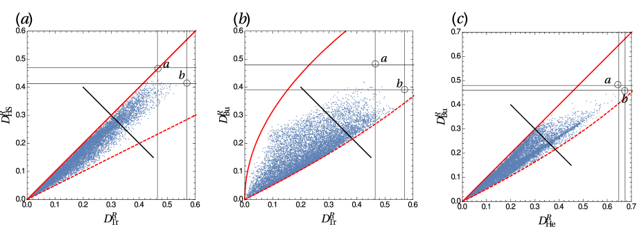
Figure 2: (a) Values of the Hilbert-Schmidt and trace discords of response $D^{\rm R}_{\rm HS}$ and $D^{\rm R}_{\operatorname{tr}}$ for $10^{4}$ random two-qubit states with the same fixed purity $P=0.6$. These states are generated from random spectra and eigenvectors given by the column vectors of a unitary matrix distributed according to the Haar measure. States on the thick black line have a hierarchy with respect to $D^{\rm R}_{{\rm HS}}$ that is reversed compared to the hierarchy with respect to $D^{\rm R}_{\operatorname{tr}}$. The points $a$ and $b$ represent, respectively, some states with purity $P$ maximizing $D^{\rm R}_{\rm HS}$ and $D^{\rm R}_{\operatorname{tr}}$. Note that $a$ has not maximal trace discord of response $D^{\rm R}_{\operatorname{tr}}$, and similarly for $b$ and $D^{\rm R}_{\rm HS}$. (b) Same for the Bures and trace discords of response $D^{\rm R}_{\rm Bu}$ and $D^{\rm R}_{\operatorname{tr}}$. (c) Same for the Bures and Hellinger discords of response $D^{\rm R}_{\rm Bu}$ and $D^{\rm R}_{{\rm He}}$. The solid and dashed lines are the borders of the regions delimited by bounds on $D^{\rm R}$ derived from Table 3 below. This figure is taken from Ref. [78].

4 Bures and Hellinger distances

In this section we review the properties of the Bures and Hellinger distances between quantum states.

4.1 Bures distance

The Bures distance was first introduced by Bures in the context of infinite products of von Neumann algebras [19] (see also [4]) and was later studied in a series of papers by Uhlmann [92, 93]. Uhlmann used it to define parallel transport and related it to the fidelity generalizing the usual fidelity $|\langle\psi|\phi\rangle|^{2}$ between pure states. Indeed, the Bures distance is an extension to mixed states of the Fubini-Study distance for pure states. Recall that the pure states $\rho_{\psi}=|\psi\rangle\langle\psi|$ of a quantum system with Hilbert space ${\cal H}$ can be identified with elements of the projective space $P{\cal H}$, that is, the set of equivalence classes of normalized vectors in ${\cal H}$ modulo a phase factor. The vectors $|\psi_{\theta}\rangle=e^{{\rm{i}}\theta}|\psi\rangle\in{\cal H}$ with $0\leq\theta<2\pi$ are called the representatives of $\rho_{\psi}$. The Fubini-Study distance on $P{\cal H}$ is defined by

$$d_{\rm FS}\bigl{(}\rho_{\psi},\sigma_{\phi}\bigr{)}=\inf_{\|\psi_{\theta}\|=\|\phi_{\delta}\|=1}\bigl{\|}|\psi_{\theta}\rangle-|\phi_{\delta}\rangle\bigr{\|}=\bigl{(}2-2|\langle\psi|\phi\rangle|\bigr{)}^{\frac{1}{2}}\;,$$ (39)

where the infimum in the second member is over all representatives $|\psi_{\theta}\rangle$ of $\rho_{\psi}$ and $|\phi_{\delta}\rangle$ of $\sigma_{\phi}$. Observe that the third member depends on the equivalent classes $\rho_{\psi}$ and $\sigma_{\phi}$ only.

For two mixed states $\rho$ and $\sigma\in{\cal E}({\cal H})$, one can define analogously [93, 47]

$$d_{\rm Bu}(\rho,\sigma)=\inf_{R,S}d_{2}(R,S)\;,$$ (40)

where $d_{2}$ is the Hilbert-Schmidt distance and the infimum is over all Hilbert-Schmidt matrices $R$ and $S\in{\cal B}({\cal H})$ satisfying $RR^{\dagger}=\rho$ and $SS^{\dagger}=\sigma$. Such matrices are given by $R=\sqrt{\rho}V$ and $S=\sqrt{\sigma}W$ for some unitaries $V$ and $W$ on ${\cal H}$ (polar decompositions).

Proposition 6.

$d_{\rm Bu}$ defines a distance on the set of quantum states ${\cal E}({\cal H})$, which coincides with the Fubini-Study distance for pure states.

Proof. It is clear on (40) that $d_{\rm Bu}(\rho,\sigma)$ is symmetric, non-negative, and vanishes if and only if $\rho=\sigma$. To prove the triangle inequality, let us first observe that by the polar decomposition and the invariance property $d_{2}(RV,SV)=d_{2}(R,S)$ of the Hilbert-Schmidt distance for any unitary $V$, one has $d_{\rm Bu}(\rho,\sigma)=\inf_{U}d_{2}(\sqrt{\rho},\sqrt{\sigma}U)$ with an infimum over all unitaries $U$. Let $\rho$, $\sigma$, and $\tau$ be three states in ${\cal E}({\cal H})$. The triangle inequality for $d_{2}$ and the aforementioned invariance property yield

$$d_{\rm Bu}(\rho,\tau) \leq \inf_{U,V}\big{\{}d_{2}(\sqrt{\rho},\sqrt{\sigma}V)+d_{2}(\sqrt{\sigma}V,\sqrt{\tau}U)\big{\}}=\inf_{V}d_{2}(\sqrt{\rho},\sqrt{\sigma}V)+\inf_{W}d_{2}(\sqrt{\sigma},\sqrt{\tau}W)$$ (41)

$$= d_{\rm Bu}(\rho,\sigma)+d_{\rm Bu}(\sigma,\tau)\;.$$

Hence $d_{\rm Bu}$ defines a distance on ${\cal E}({\cal H})$. For pure states $\rho_{\psi}=|\psi\rangle\langle\psi|$ and $\sigma_{\phi}=|\phi\rangle\langle\phi|$, the Hilbert-Schmidt operators are of the form $R=|\psi\rangle\langle\mu|$ and $S=|\phi\rangle\langle\nu|$ with $\|\mu\|=\|\nu\|=1$. A simple calculation then shows that the r.h.s.  of (39) and (40) coincide. $\Box$

By using the polar decompositions and the formula $\|O\|_{1}=\sup_{U}\mathrm{Re}\,\operatorname{tr}(UO)$ for the trace norm $\|\cdot\|_{1}$ (the supremum is over all unitaries $U$), one finds

$$d_{\rm Bu}(\rho,\sigma)=\bigl{(}2-2\sup_{U}\mathrm{Re}\,\operatorname{tr}(U\sqrt{\rho}\sqrt{\sigma})\bigr{)}^{\frac{1}{2}}=\bigl{(}2-2\sqrt{F(\rho,\sigma)}\bigr{)}^{\frac{1}{2}}\;,$$ (42)

where $F(\rho,\sigma)=\|\sqrt{\rho}\sqrt{\sigma}\|_{1}^{2}$ is the Uhlmann fidelity. Furthermore, the infimum in (40) is attained if and only if  the parallel transport condition $R^{\dagger}S\geq 0$ holds.

Since the fidelity $F(\rho,\sigma)$ belongs to $[0,1]$, $d_{\rm Bu}(\rho,\sigma)$ takes values in the interval $[0,\sqrt{2}]$. Two states $\rho$ and $\sigma$ have a maximal distance $d_{\rm Bu}(\rho,\sigma)=\sqrt{2}$ (i.e., a vanishing fidelity $F(\rho,\sigma)$) if and only if  they have orthogonal supports, $\operatorname{ran}\rho\,{\bot}\,\operatorname{ran}\sigma$. Such orthogonal states are thus perfectly distinguishable.

Comparing (39) and (42), one sees that the Uhlmann fidelity $F$ is a generalization of the usual pure state fidelity $F(|\psi\rangle,|\phi\rangle)=|\langle\psi|\phi\rangle|^{2}$. More generally, if $\sigma_{\phi}$ is pure, then it follows from (17) that

$$F(\rho,\sigma_{\phi})=\langle\phi|\rho|\phi\rangle$$ (43)

for any $\rho\in{\cal E}({\cal H})$. A very useful result due to Uhlmann shows that for any states $\rho$ and $\sigma$, $F(\rho,\sigma)$ is equal to the fidelity between two pure states $|\Psi\rangle$ and $|\Phi\rangle$ belonging to an enlarged space ${\cal H}\otimes{\cal K}$ and having marginals $\rho=\operatorname{tr}_{\cal K}(|\Psi\rangle\langle\Psi|)$ and $\sigma=\operatorname{tr}_{\cal K}(|\Phi\rangle\langle\Phi|)$. Such states $|\Psi\rangle$ and $|\Phi\rangle$ are called purifications of $\rho$ and $\sigma$ on ${\cal H}\otimes{\cal K}$. More precisely, one has

Theorem 2.

[92] Let $\rho$, $\sigma\in{\cal E}({\cal H})$ and $|\Psi\rangle$ be a purification of $\rho$ on the Hilbert space ${\cal H}\otimes{\cal K}$, with $\dim{\cal K}\geq\dim{\cal H}$. Then

$$F(\rho,\sigma)=\max_{|\Phi\rangle}|\langle\Psi|\Phi\rangle|^{2}\;,$$ (44)

where the maximum is over all purifications $|\Phi\rangle$ of $\sigma$ on ${\cal H}\otimes{\cal K}$.

Proof. Let us first assume ${\cal K}={\cal H}$. Then (44) follows from the definition (40) of the Bures distance and the fact that the map $R\mapsto|\Psi_{R}\rangle=\sum_{i,j}\langle i|R|j\rangle|i\rangle|j\rangle$ is an isometry between ${\cal B}({\cal H})$ (endowed with the Hilbert-Schmidt norm $\|\cdot\|_{2}$) and ${\cal H}\otimes{\cal H}$ (here $\{|i\rangle\}$ is some fixed orthonormal basis  of ${\cal H}$). Indeed, one easily checks that $\rho=RR^{\dagger}$ if and only if $|\Psi_{R}\rangle$ is a purification of $\rho$ on ${\cal H}\otimes{\cal H}$. Hence, using (39), (40), and the invariance property of $d_{2}$ mentioned in the proof of Proposition 6, one has

$$d_{\rm Bu}(\rho,\sigma)^{2}=\inf_{S}\big{\|}R-S\big{\|}_{2}^{2}=\inf_{|\Phi_{S}\rangle}\big{\|}|\Psi_{R}\rangle-|\Phi_{S}\rangle\big{\|}^{2}=\inf_{|\Phi_{S}\rangle}d_{\rm FS}\big{(}|\Psi_{R}\rangle,|\Phi_{S}\rangle\big{)}^{2}=2-2\sup_{|\Phi_{S}\rangle}|\langle\Psi_{R}|\Phi_{S}\rangle|\;,$$

where the infimum and supremum are over all purifications $|\Phi_{S}\rangle$ of $\sigma$ on ${\cal H}\otimes{\cal H}$, and are actually minimum and maximum.

If $\dim{\cal K}>\dim{\cal H}$, we extend $\rho$ and $\sigma$ to a larger space ${{\cal H}}^{\prime}\simeq{\cal K}$ by adding to them new orthonormal eigenvectors with zero eigenvalues. As is clear from (42), this does not change the distance, hence $d_{\rm B}(\rho,\sigma)=\inf_{{R}^{\prime},{S}^{\prime}}d_{2}({R}^{\prime},{S}^{\prime})$ with an infimum over all ${R}^{\prime},{S}^{\prime}\in{\cal B}({{\cal H}}^{\prime})$ such that ${R}^{\prime}({R}^{\prime})^{\dagger}$ and ${S}^{\prime}({S}^{\prime})^{\dagger}$ are equal to the extensions of $\rho$ and $\sigma$. But ${R}^{\prime}$ and ${S}^{\prime}$ can be viewed as operators from ${\cal K}$ to ${\cal H}$ since they have ranges $\operatorname{ran}{R}^{\prime}=\ker({R}^{\prime})^{\dagger}$ and $\operatorname{ran}{S}^{\prime}=\ker({S}^{\prime})^{\dagger}$ included in ${\cal H}$. Thus, one can take the infimum in (40) over all operators $R,S:{\cal K}\rightarrow{\cal H}$ such that $RR^{\dagger}=\rho$ and $SS^{\dagger}=\sigma$, without changing the result. The formula (44) then follows from the same argument as above, using the fact that $R\mapsto|\Psi_{R}\rangle$ is an isometry between the Hilbert space of all operators ${\cal K}\rightarrow{\cal H}$ and ${\cal H}\otimes{\cal K}$. $\Box$

A direct proof of (44) from the definition $F(\rho,\sigma)=\|\sqrt{\rho}\sqrt{\sigma}\|_{1}^{2}$ of the fidelity has been given Ref. [50] (see also [64]). As the fidelity satisfies $F(\rho_{A}\otimes\rho_{B},\sigma_{A}\otimes\sigma_{B})=F(\rho_{A},\sigma_{A})F(\rho_{B},\sigma_{B})$, the Bures distance increases by taking tensor products, i.e.,

$$d_{\rm Bu}(\rho_{A}\otimes\rho_{B},\sigma_{A}\otimes\sigma_{B})\geq d_{\rm Bu}(\rho_{A},\sigma_{A})$$ (45)

with equality if and only if  $\rho_{B}=\sigma_{B}$. Note that the trace distance does not enjoy this property.

4.2 Classical and quantum Hellinger distances

Let ${\cal E}_{\rm clas}=\{{\bf{p}}\in{\mathbb{R}}_{+}^{n};\sum_{k}p_{k}=1\}$ be the simplex of classical probability distributions on the finite sample space $\{1,2,\ldots,n\}$. The restriction of a distance $d$ on ${\cal E}({\cal H})$ to all density matrices commuting with a given state $\rho_{0}$ defines a distance on ${\cal E}_{\rm clas}$. In particular, if $\rho$ and $\sigma$ are two commuting states with spectral decompositions $\rho=\sum_{k}p_{k}|k\rangle\langle k|$ and $\sigma=\sum_{k}q_{k}|k\rangle\langle k|$, then

$$d_{\rm Bu}(\rho,\sigma)=d_{\rm clas}({\bf{p}},{\bf{q}})\equiv\Bigl{(}2-2\sum_{k=1}^{n}\sqrt{p_{k}q_{k}}\Bigr{)}^{\frac{1}{2}}=\biggl{(}\sum_{k=1}^{n}(\sqrt{p_{k}}-\sqrt{q_{k}})^{2}\biggr{)}^{\frac{1}{2}}$$ (46)

reduces to the classical Hellinger distance $d_{\rm clas}$ on ${\cal E}_{\rm clas}$. One can of course define other distances on ${\cal E}({\cal H})$ which coincide with $d_{\rm clas}$ for commuting density matrices, by choosing a different ordering of the operators inside the trace in the definition (17) of the fidelity. For the “normal ordering”, one obtains the quantum Hellinger distance

$$d_{{\rm He}}(\rho,\sigma)=\big{(}2-2\operatorname{tr}\sqrt{\rho}\sqrt{\sigma}\big{)}^{\frac{1}{2}}=d_{2}(\sqrt{\rho},\sqrt{\sigma})\;.$$ (47)

Since $d_{2}$ is a distance on ${\cal E}({\cal H})$, this is also the case for $d_{{\rm He}}$. In the sequel, $d_{{\rm He}}$ will be referred to as the Hellinger distance when it is clear from the context that one works with quantum states and not probability distributions.

Comparing (40) and (47), one immediately sees that $d_{\rm He}(\rho,\sigma)\geq d_{\rm Bu}(\rho,\sigma)$ for any states $\rho,\sigma\in{\cal E}({\cal H})$. Like $d_{\rm Bu}$, the Hellinger distance satisfies the monotonicity (45) under tensor products. A notable difference between $d_{\rm Bu}$ and $d_{\rm He}$ is that the latter does not coincide with the Fubini-Study distance for pure states (in fact, $d_{\rm He}(\rho_{\psi},\sigma_{\phi})=(2-2|\langle\psi|\phi\rangle|^{2})^{\frac{1}{2}}>d_{\rm FS}(\rho_{\psi},\sigma_{\phi})$ if $\rho_{\psi}$ and $\sigma_{\phi}$ are distinct and non-orthogonal).

One can associate to two non-commuting states $\rho$ and $\sigma$ the probabilities ${\bf{p}}=(p_{1},\cdots,p_{m})$ and ${\bf{q}}=(q_{1},\cdots,q_{m})$ of the outcomes of a measurement performed on the system respectively in states $\rho$ and $\sigma$. A natural question is whether $d_{\rm Bu}(\rho,\sigma)$ or $d_{\rm He}(\rho,\sigma)$ coincide with the supremum of the classical distance $d_{\rm clas}({\bf{p}},{\bf{q}})$ over all such measurements.

Proposition 7.

For any $\rho,\sigma\in{\cal E}({\cal H})$, one has

$$d_{\rm Bu}(\rho,\sigma)=\sup_{\{M_{i}\}}d_{\rm clas}({\bf{p}},{\bf{q}})\;,$$ (48)

where the supremum is over all POVMs $\{M_{i}\}_{i=1}^{m}$ and $p_{i}=\operatorname{tr}M_{i}\rho$ (respectively $q_{i}=\operatorname{tr}M_{i}\sigma$) is the probability of the measurement outcome $i$ in the state $\rho$ (respectively $\sigma$). The supremum is achieved for von Neumann measurements with rank-one projectors $M_{i}=|i\rangle\langle i|$.

A proof of this result and references to the original works can be found in Nielsen and Chuang’s book [64]. Note that a similar statement also holds for the trace distance (with $d_{\rm clas}$ replaced by the $\ell^{1}$-distance). In contrast, while $d_{\rm clas}({\bf{p}},{\bf{q}})\leq d_{\rm Hel}(\rho,\sigma)$ for any POVM, the maximum over all POVMs is strictly smaller than $d_{\rm Hel}(\rho,\sigma)$, except when $d_{{\rm He}}(\rho,\sigma)=d_{\rm Bu}(\rho,\sigma)$.

4.3 Contractivity and joint convexity

Proposition 8.

The Bures and Hellinger distances $d_{\rm Bu}$ and $d_{\rm He}$ are contractive under quantum operations. Moreover, $d_{\rm Bu}^{2}$ and $d_{\rm He}^{2}$ are jointly convex, that is,

$$d_{\rm Bu}^{2}\Bigl{(}\sum_{i}p_{i}\rho_{i},\sum_{i}p_{i}\sigma_{i}\Bigr{)}\leq\sum_{i}p_{i}d_{\rm Bu}^{2}(\rho_{i},\sigma_{i})\;,$$ (49)

with a similar inequality for $d_{\rm He}$.

The relative entropy $S(\rho||\sigma)$ is also jointly convex. This mathematical property is interpreted as follows. Given two ensembles $\{\rho_{i},p_{i}\}$ and $\{\sigma_{i},p_{i}\}$ of states in ${\cal E}({\cal H})$ with the same probabilities $p_{i}$, by erasing the information about which state of the ensemble is chosen, the state of the system becomes $\rho=\sum_{i}p_{i}\rho_{i}$ or $\sigma=\sum_{i}p_{i}\sigma_{i}$. The joint convexity means that the entropy between the two ensembles after the loss of information provoked by the state mixing is smaller or equal to the average of the entropies $S(\rho_{i}||\sigma_{i})$. Note that the $L^{p}$-distances $d_{p}$ also fulfill this requirement. According to Proposition 8, the same is true for the squares of the Bures and Hellinger distances, but not for the distances themselves.

The contractivity of $d_{\rm He}$ will be deduced from the following more general result, known as Lieb’s concavity theorem [51] (see e.g. [64] for a proof). We denote by ${\cal{B}}({\cal{H}})_{+}$ the set of all non-negative operators on ${\cal H}$.

Theorem 3.

[51] For any fixed operator $K\in{\cal{B}}({\cal{H}})$, $\beta\in[-1,0]$, and $q\in[0,1+\beta]$, the function $(\rho,\sigma)\mapsto\operatorname{tr}(K^{\dagger}\rho^{q}K\sigma^{-\beta})$ on ${\cal{B}}({\cal{H}})_{+}\times{\cal{B}}({\cal{H}})_{+}$ is jointly concave in $(\rho,\sigma)$.

Proof of Proposition 8. Let us first show that $d_{\rm Bu}^{2}$ is jointly convex. This is a consequence of the bound

$$\sqrt{F\Bigl{(}\sum_{i}p_{i}\rho_{i},\sum_{i}q_{i}\sigma_{i}\Bigr{)}}\geq\sum_{i}\sqrt{p_{i}q_{i}}\sqrt{F(\rho_{i},\sigma_{i})}\;.$$ (50)

To establish (50), we use Theorem 2 and introduce some purifications $|\Psi_{i}\rangle$ of $\rho_{i}$ and $|\Phi_{i}\rangle$ of $\sigma_{i}$ on ${\cal H}\otimes{\cal H}$ such that $\sqrt{F(\rho_{i},\sigma_{i})}=|\langle\Psi_{i}|\Phi_{i}\rangle|=\langle\Psi_{i}|\Phi_{i}\rangle$. Let us define the vectors

$$|\Psi\rangle=\sum_{i}\sqrt{p_{i}}|\Psi_{i}\rangle|i\rangle\quad,\quad|\Phi\rangle=\sum_{i}\sqrt{p_{i}}|\Phi_{i}\rangle|i\rangle$$ (51)

in ${\cal H}\otimes{\cal H}\otimes{\cal H}_{E}$, where ${\cal H}_{E}$ is an auxiliary Hilbert space with orthonormal basis  $\{|i\rangle\}$. Then $|\Psi\rangle$ and $|\Phi\rangle$ are purifications of $\rho=\sum_{i}p_{i}\rho_{i}$ and $\sigma=\sum_{i}q_{i}\sigma_{i}$, respectively. Using Theorem 2 again, one finds

$$\sqrt{F(\rho,\sigma)}\geq|\langle\Psi|\Phi\rangle|=\sum_{i}\sqrt{p_{i}q_{i}}\langle\Psi_{i}|\Phi_{i}\rangle=\sum_{i}\sqrt{p_{i}q_{i}}\sqrt{F(\rho_{i},\sigma_{i})}\;.$$ (52)

We have thus proven that $d_{\rm Bu}^{2}$ is jointly convex. The joint convexity of $d_{\rm He}^{2}$ is a corollary of Theorem 3, which insures that $(\rho,\sigma)\mapsto\operatorname{tr}(\sqrt{\rho}\sqrt{\sigma})$ is jointly concave.

The following general argument shows that the contractivity of $d_{\rm Bu}$ and $d_{\rm He}$ is a consequence of the joint convexity proven above and of Stinespring’s theorem [84] on CP maps [91, 99, 31]. Recall that if $\mu_{\rm H}$ is the normalized Haar measure on the group $U(n)$ of $n\times n$ unitary matrices, then $\int{\rm{d}}\mu_{\rm H}(U)\,UBU^{\dagger}=n^{-1}\operatorname{tr}B$ for any $B\in{\cal{B}}({\cal{H}})$ (in fact, all diagonal matrix elements of $O=\int{\rm{d}}\mu_{\rm H}(U)\,UBU^{\dagger}$ in an arbitrary basis are equal, as a result of the left-invariance of the Haar measure, ${\rm{d}}\mu_{\rm H}(VU)={\rm{d}}\mu_{\rm H}(U)$ for any $V\in U(n)$; thus $O$ is proportional to the identity matrix). Let ${\cal M}$ be a quantum operation  on ${\cal{B}}({\cal{H}})$. One infers from the Stinespring theorem that there exists a pure state $|\epsilon_{0}\rangle$ of an ancilla system ${E}$ and a unitary $U$ on ${\cal H}\otimes{\cal H}_{E}$ such that

$${\cal M}(\rho)\otimes(1/n_{E})=\operatorname{tr}_{E}(U\rho\otimes|\epsilon_{0}\rangle\langle\epsilon_{0}|U^{\dagger})\otimes(1/n_{E})=\int{\rm{d}}\mu_{\rm H}(U_{E})\,(1\otimes U_{E})U\rho\otimes|\epsilon_{0}\rangle\langle\epsilon_{0}|U^{\dagger}(1\otimes U_{E}^{\dagger})\;.$$ (53)

By using the property $d_{\rm Bu}(\rho\otimes\tau,\sigma\otimes\tau)=d_{\rm Bu}(\rho,\sigma)$, see (45), and the joint convexity and unitary invariance of $d_{\rm Bu}^{2}$, one gets

$$d_{\rm Bu}^{2}({\cal M}(\rho),{\cal M}(\sigma))=d_{\rm Bu}^{2}\bigl{(}{\cal M}(\rho)\otimes(1/n_{E})\,,\,{\cal M}(\sigma)\otimes(1/n_{E})\bigr{)}$$

$$\hskip 28.45274pt\leq\int{\rm{d}}\mu_{\rm H}(U_{E})d_{\rm Bu}^{2}\bigl{(}(1\otimes U_{E})U\rho\otimes|\epsilon_{0}\rangle\langle\epsilon_{0}|U^{\dagger}(1\otimes U_{E}^{\dagger})\,,\,(1\otimes U_{E})U\sigma\otimes|\epsilon_{0}\rangle\langle\epsilon_{0}|U^{\dagger}(1\otimes U_{E}^{\dagger})\bigr{)}$$

$$\hskip 28.45274pt=\int{\rm{d}}\mu_{\rm H}(U_{E})d_{\rm Bu}^{2}(\rho,\sigma)=d_{\rm Bu}^{2}(\rho,\sigma)\;.$$ (54)

A similar reasoning applies to $d_{\rm He}$. $\Box$

4.4 Riemannian metrics

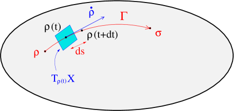
Figure 3: Curve $\Gamma$ joining two states $\rho$ and $\sigma$ in the set of quantum states $X={\cal E}({\cal H})$.

In Riemannian geometry, a metric on a smooth manifold $X$ is a (smooth) map $g$ associating to each point $x$ in $X$ a scalar product $g_{x}$ on the tangent space $T_{x}X$ at $x$. A metric $g$ induces a Riemannian distance $d$, which is such that the square distance ${\rm{d}}s^{2}=d(x,x+{\rm{d}}x)^{2}$ between two infinitesimally close points $x$ and $x+{\rm{d}}x$ is equal to $g_{x}({\rm{d}}x,{\rm{d}}x)$. For the manifold $X={\cal E}({\cal H})$ of quantum states, the tangent spaces $T_{\rho}{\cal E}({\cal H})$ can be identified with the (real) vector space ${\cal{B}}({\cal{H}})_{\rm s.a.}^{0}$ of self-adjoint operators on ${\cal H}$ with zero trace. A curve $\Gamma$ in ${\cal E}({\cal H})$ joining two states $\rho_{0}$ and $\rho_{1}$ is a (continuously differentiable) map $\Gamma:t\in[0,1]\mapsto\rho(t)\in{\cal E}({\cal H})$ with $\Gamma(0)=\rho_{0}$ and $\Gamma(1)=\rho_{1}$ (see Fig. 3). Its length $\ell(\Gamma)$ is

$$\ell(\Gamma)=\int_{\Gamma}{\rm{d}}s=\int_{0}^{1}{\rm{d}}t\,\sqrt{g_{\rho(t)}(\dot{\rho}(t),\dot{\rho}(t))}\;,$$ (55)

where $\dot{\rho}(t)$ stands for the time derivative ${\rm{d}}\rho/{\rm{d}}t$. A curve $\Gamma_{\rm g}(\rho,\sigma)$ joining $\rho$ and $\sigma$ with the shortest length, or more generally a curve $\Gamma_{\rm g}(\rho,\sigma)\in{\cal C}(\rho,\sigma)=\{\Gamma\in C^{1}([0,1],{\cal E}({\cal H}));\Gamma(0)=\rho,\Gamma(1)=\sigma\}$ at which the map $\Gamma\in{\cal C}(\rho,\sigma)\mapsto\ell(\Gamma)$ has a stationary point, is called a geodesic. The distance between two states $\rho$ and $\sigma$ is the length of the shortest geodesic joining $\rho$ and $\sigma$, $d(\rho,\sigma)=\min\{\ell(\Gamma_{\rm g}(\rho,\sigma))\}=\min_{\Gamma\in{\cal C}(\rho,\sigma)}\ell(\Gamma)$. Thanks to this formula, a distance $d$ on ${\cal E}({\cal H})$ can be associated to any metric $g$. Conversely, one can associate a metric $g$ to a distance $d$ if the following condition is satisfied (we ignore here the regularity assumptions): for any $\rho\in{\cal E}({\cal H})$ and $\dot{\rho}\in{\cal{B}}({\cal{H}})_{\rm s.a.}^{0}$, the square distance between $\rho$ and $\rho+t\dot{\rho}$ has a small time Taylor expansion of the form

$${\rm{d}}s^{2}=d(\rho,\rho+t\dot{\rho})^{2}=g_{\rho}(\dot{\rho},\dot{\rho})t^{2}+{\cal O}(t^{3})\;.$$ (56)

Needless to say, determining the metric induced by a given distance $d$ is much simpler than finding an explicit formula for $d(\rho,\sigma)$ for arbitrary states $\rho,\sigma\in{\cal E}({\cal H})$ from the expression of the metric $g$.

A trivial example of metric on ${\cal E}({\cal H})$ is

$$g_{\rho}(O,O^{\prime})=\langle O,O^{\prime}\rangle=\operatorname{tr}(OO^{\prime})\quad,\quad O,O^{\prime}\in{\cal{B}}({\cal{H}})_{\rm s.a.}^{0}\;,$$ (57)

i.e., $g_{\rho}$ is independent of $\rho$ and given by the Hilbert-Schmidt scalar product for matrices. Introducing an orthonormal basis  $\{|i\rangle\}_{i=1}^{n}$ of ${\cal H}$, one finds that $g_{\rho}(O,O^{\prime})=\sum_{i,j=1}^{n}\overline{O_{ij}}O_{ij}^{\prime}$ is nothing but the Euclidean scalar product. Thus the geodesics are straight lines, $\Gamma_{\rm g}(\rho,\sigma):t\in[0,1]\mapsto(1-t)\rho+t\sigma$, and the distance between two arbitrary states $\rho$ and $\sigma$ is the Hilbert-Schmidt distance $d_{2}(\rho,\sigma)=\langle-\rho+\sigma,-\rho+\sigma\rangle^{\frac{1}{2}}=(\operatorname{tr}[(\rho-\sigma)^{2}])^{\frac{1}{2}}$.

It is not difficult to show (see [83]) that the Bures and Hellinger distances are Riemannian and have metrics given by

$$\begin{array}[]{ccc}(g_{\rm Bu})_{\rho}(O,O)&=&\displaystyle\frac{1}{2}\sum_{k,l=1}^{n}\frac{|\langle k|O|l\rangle|^{2}}{p_{k}+p_{l}}\\ (g_{\rm He})_{\rho}(O,O)&=&\displaystyle\sum_{k,l=1}^{n}\frac{|\langle k|O|l\rangle|^{2}}{(\sqrt{p_{k}}+\sqrt{p_{l}})^{2}}\end{array}\quad,\quad O\in{\cal{B}}({\cal{H}})_{\rm s.a.}^{0}\;,\;\rho>0\;,$$ (58)

where $\{|k\rangle\}$ is an orthonormal basis  of eigenvectors of $\rho$ with eigenvalues $p_{k}$. In contrast, the trace distance $d_{1}$ is not Riemannian. One deduces from (58) that

$$(g_{\rm Bu})_{\rho}(O,O)\leq(g_{\rm He})_{\rho}(O,O)\leq 2(g_{\rm Bu})_{\rho}(O,O)\;.$$ (59)

The volume of ${\cal E}({\cal H})$ and the area of its boundary for the Bures metric have been determined in Ref. [80].

4.5 Physical interpretations of the Bures and Hellinger metrics

The metrics $g_{\rm Bu}$ and $g_{\rm He}$ have interpretations in quantum metrology and quantum hypothesis testing. Let us first discuss the link with quantum metrology. Consider the curve in ${\cal E}({\cal H})$ given by the unitary evolution of the state $\rho(0)=\rho$ under the Hamiltonian $H\in{\cal{B}}({\cal{H}})_{\rm s.a.}$,

$$\rho(t)=e^{-{\rm{i}}tH}\rho\,e^{{\rm{i}}tH}\;.$$ (60)

Then $\dot{\rho}(t)=-{\rm{i}}[H,\rho(t)]$. Assuming that $\rho$ is invertible, the speed of the state evolution, $v(t_{0})=\lim_{t\rightarrow 0}t^{-1}d_{\rm Bu}(\rho(t_{0}),\rho(t_{0}+t))$, is given by $\sqrt{{\cal F}_{Q}(\rho(t_{0}),H)}/2=\sqrt{{\cal F}_{Q}(\rho,H)}/2$, where

$${\cal F}_{Q}(\rho,H)=4(g_{\rm Bu})_{\rho}\bigl{(}-{\rm{i}}[H,\rho],-{\rm{i}}[H,\rho]\bigr{)}=2\sum_{k,l,p_{k}+p_{l}>0}\frac{(p_{k}-p_{l})^{2}}{p_{k}+p_{l}}|\langle k|H|l\rangle|^{2}$$ (61)

is the quantum Fisher information. This quantity is related to the smallest error $\Delta t$ that can be achieved when estimating the unknown parameter $t$ by performing measurements on the output states $\rho(t)$. Indeed, optimizing over all measurements and all unbiased statistical estimators (that is, all functions $t_{\rm est}(i_{1},\cdots,i_{N})$ depending on the measurement outcomes $i_{1},\cdots,i_{N}$ and such that $\langle t_{\rm est}\rangle=t$), the best precision is given by [17]

$$(\Delta t)_{\rm{best}}=\frac{1}{\sqrt{N}\sqrt{{\cal F}_{Q}(\rho,H)}}\;,$$ (62)

where $N$ is the number of measurements. Note that for pure states ${\cal F}_{Q}(|\psi\rangle,H)=4\langle(\Delta H)^{2}\rangle_{\psi}$ reduces to the square quantum fluctuation $\langle(\Delta H)^{2}\rangle_{\psi}=\langle\psi|H^{2}|\psi\rangle-\langle\psi|H|\psi\rangle^{2}$ up to a factor of four. Hence (62) takes the form of a generalized uncertainty relation $(\Delta t)^{2}\langle(\Delta H)^{2}\rangle_{\psi}\geq 1/4$ (here we take $N=1$), in which $H$ plays the role of the variable conjugated to the parameter $t$. We remark that the second equality in (61) is only valid when $\rho>0$. The quantum Fisher information is, however, given by the last expression in (61) for any state $\rho$.

The analog of (61) for the Hellinger metric is the skew information [97]

$${\cal I}_{\rm skew}(\rho,H)=\frac{1}{2}(g_{\rm He})_{\rho}\bigl{(}-{\rm{i}}[H,\rho],-{\rm{i}}[H,\rho]\bigr{)}=-\frac{1}{2}\operatorname{tr}\big{(}[\sqrt{\rho}\,,\,H]^{2}\bigr{)}\;.$$ (63)

It describes the amount of information on the values of observables not commuting with $H$ in a system in state $\rho$. The Fisher and skew informations have the following properties [97, 53]:

• they are non-negative and vanish if and only if  $[\rho,H]=0$ (this follows from the fact that $(g_{\rm Bu})_{\rho}$ and $(g_{\rm He})_{\rho}$ are scalar products);

• they are convex in $\rho$ (this follows from the joint convexity of $d_{\rm Bu}^{2}$ and $d_{\rm He}^{2}$).

• they are additive, i.e., ${\cal F}_{Q}(\rho_{A}\otimes\rho_{B},H_{A}\otimes 1+1\otimes H_{B})={\cal F}_{Q}(\rho_{A},H_{A})+{\cal F}_{Q}(\rho_{B},H_{B})$, with a similar identity for ${\cal I}_{\rm skew}$;

• the Fisher information is given by [30, 90]

  $$\frac{1}{4}{\cal F}_{Q}(\rho,H)=\inf_{\{|\psi_{i}\rangle,\eta_{i}\}}\bigg{\{}\sum_{i}\eta_{i}\langle(\Delta H)^{2}\rangle_{\psi_{i}}\bigg{\}}\;,$$ (64)

  where the infimum is over all pure state decompositions $\rho=\sum_{i}\eta_{i}|\psi_{i}\rangle\langle\psi_{i}|$ of $\rho$;

• they obey the bounds

  $$\frac{1}{8}{\cal F}_{Q}(\rho,H)\leq{\cal I}_{\rm skew}(\rho,H)\leq\frac{1}{4}{\cal F}_{Q}(\rho,H)\leq\langle(\Delta H)^{2}\rangle_{\rho}\;,$$ (65)

  where $\langle(\Delta H)^{2}\rangle_{\rho}=\operatorname{tr}(\rho H^{2})-(\operatorname{tr}\rho H)^{2}$ is the variance of $H$. The second and third inequalities are equalities for pure states.

It can be shown that if the system is composed of $N_{\rm p}$ particles, $H$ is the sum of the same single particle Hamiltonian $H_{{\rm 1p}}$ acting on each particle, and $\Delta h$ is the half difference between the maximal and minimal eigenvalues of $H_{{\rm 1p}}$, then ${\cal F}_{Q}(\rho,H)>4(\Delta h)^{2}N_{\rm p}$ is a sufficient (but not necessary) condition for particle entanglement [72, 83]. Furthermore, high values of ${\cal F}_{Q}({\rho},H)$ imply multipartite entanglement between a large number of particles [48, 89].

Let us now discuss the link with the hypothesis testing problem. This problem consists in discriminating two probability measures $\mu_{1}$ and $\mu_{2}$ given the outcomes of $N$ independent identically distributed random variables with laws given by either $\mu_{1}$ or $\mu_{2}$. In the quantum setting, this is rephrased as a discrimination of two states $\rho$ and $\sigma$ given $N$ independent copies of $\rho$ and $\sigma$, by means of measurements on the $N$ copies either in state $\rho^{\otimes N}$ or $\sigma^{\otimes N}$. One decides among the two alternatives according to the two possible measurement  outcomes. According to the quantum Chernoff bound [5, 65], the probability of error decays exponentially in the limit $N\rightarrow\infty$, with a rate given by a contractive function $\xi(\rho,\sigma)$, which is equal to $g_{\rm He}({\rm{d}}\rho,{\rm{d}}\rho)/2$ for two infinitesimally close states $\rho$ and $\sigma=\rho+{\rm{d}}\rho$.

4.6 Characterization of all Riemannian contractive distances

In Ref. [70], Petz has determined the general form of all Riemannian contractive distances on ${\cal E}({\cal H})$ for finite-dimensional Hilbert spaces ${\cal H}$. Such distances are induced by metrics $g$ satisfying

$$g_{{\cal M}(\rho)}\bigl{(}{\cal M}(O),{\cal M}(O)\bigr{)}\leq g_{\rho}(O,O)\quad,\quad O\in{\cal{B}}({\cal{H}})_{\rm s.a.}^{0}\;,$$ (66)

for any $\rho\in{\cal E}({\cal H})$ and any quantum operation  ${\cal M}:{\cal B}({\cal H})\rightarrow{\cal B}({\cal H}^{\prime})$. We recall that a real function $f:{\mathbb{R}}_{+}\rightarrow{\mathbb{R}}$ is operator monotone-increasing if for any space dimension $n=\dim{\cal H}<\infty$ and any $A,B\in{\cal B}({\cal H})_{+}$, one has $A\leq B\Rightarrow f(A)\leq f(B)$ (see e.g. [16]).

Theorem 4.

[70] Any continuous contractive metric $g$ on ${\cal E}({\cal H})$ has the form

$$g_{\rho}(O,O)=\sum_{k,l=1}^{n}c(p_{k},p_{l})|\langle k|O|l\rangle|^{2}\quad,\quad O\in{\cal{B}}({\cal{H}})_{\rm s.a.}^{0}\;,$$ (67)

where $\rho=\sum_{k}p_{k}|k\rangle\langle k|$ is a spectral decomposition of $\rho$,

$$c(p,q)=\frac{pf(q/p)+qf(p/q)}{2pqf(p/q)f(q/p)}\;,$$ (68)

and $f:{\mathbb{R}}_{+}\rightarrow{\mathbb{R}}_{+}$ is an operator monotone-increasing function satisfying $f(x)=xf(x^{-1})$. Conversely, the metric defined by (67) are contractive for any function $f$ with these properties. The Bures distance is the smallest of all contractive Riemannian distances with metrics satisfying the normalization condition $g_{\rho}(1,1)=\operatorname{tr}(\rho^{-1})/4$.

This theorem is of fundamental importance in geometrical approaches to quantum information. It relies on the fact that from the classical side, there exists only one (up to a normalization factor) contractive metric on the probability simplex ${\cal E}_{\rm clas}$, namely the Fisher metric ${\rm{d}}s^{2}_{\rm Fisher}=\sum_{k=1}^{n}{\rm{d}}p_{k}^{2}/p_{k}$ [21]. The metric ${\rm{d}}s^{2}_{\rm Fisher}$ plays a crucial role in statistics. It induces the Hellinger distance (46) up to a factor of one fourth. Therefore, all contractive Riemannian distances on ${\cal E}({\cal H})$ satisfying the normalization condition $g_{\rho}(1,1)=\operatorname{tr}(\rho^{-1})/4$ coincide with the classical Hellinger distance for commuting density matrices.

It can be shown that the following functions are operator monotone-increasing:

$$f_{\rm KM}(x)=4\frac{x-1}{\ln x}\;\;\leq\;\;f_{\rm He}(x)=(1+\sqrt{x})^{2}\;\;\leq\;\;f_{\rm Bu}(x)=2(x+1)\;.$$ (69)

Substituting them into the formula (68), we get

$$c_{\rm KM}(p,q)=\frac{\ln p-\ln q}{4(p-q)}\;\;\geq\;\;c_{\rm He}(p,q)=\frac{1}{(\sqrt{p}+\sqrt{q})^{2}}\;\;\geq\;\;c_{\rm Bu}(p,q)=\frac{1}{2(p+q)}\;.$$ (70)

In view of (58), the last choice $f_{\rm Bu}$ gives the Bures metrics and $f_{\rm He}$ gives the Hellinger metric.

The first choice in (69) corresponds to the so-called Kubo-Mori (or Bogoliubov) metric, which is associated to the relative entropy. In fact, an explicit calculation gives [83]

$$S(\rho+t\dot{\rho}||\rho)=\frac{t^{2}}{2}(\widetilde{g}_{\rm KM})_{\rho}(\dot{\rho},\dot{\rho})+{\cal O}(t^{3})=S(\rho||\rho+t\dot{\rho})+{\cal O}(t^{3})\;,$$ (71)

where we defined for convenience the metric $\widetilde{g}_{\rm KM}=4{g}_{\rm KM}$ satisfying the normalization condition $(\widetilde{g}_{\rm KM})_{\rho}(1,1)=\operatorname{tr}(\rho^{-1})$. As noted in [7, 8], the Kubo-Mori metric is quite natural from a physical viewpoint because ${\rm{d}}\widetilde{s}^{2}_{\rm KM}=-{\rm{d}}^{2}S$, where $S$ is the von Neumann entropy (since $S$ is concave, its second derivative is non-positive and defines a scalar product on ${\cal{B}}({\cal{H}})$). Actually, one easily deduces from (71) that

$$(\widetilde{g}_{\rm KM})_{\rho}(\dot{\rho},\dot{\rho})=-\frac{{\rm{d}}^{2}S(\rho+t\dot{\rho})}{{\rm{d}}t^{2}}\biggr{|}_{t=0}=\operatorname{tr}\dot{\rho}\,\frac{{\rm{d}}\ln(\rho+t\dot{\rho})}{{\rm{d}}t}\biggr{|}_{t=0}\;.$$ (72)

Let us consider the exponential mapping $\rho\in{\cal E}({\cal H})\mapsto O\in{\cal{B}}({\cal{H}})_{\rm s.a.}$ defined by

$$\rho=\frac{e^{O}}{\operatorname{tr}(e^{O})}\quad\Leftrightarrow\quad O-F(O)=\ln\rho\quad\text{ with }\quad F(O)=\ln(\operatorname{tr}e^{O})\;.$$ (73)

Note that $F(O)-\operatorname{tr}\rho\,O=\operatorname{tr}\rho(F(O)-O)=S(\rho)$, hence $F$ is the Legendre transform of the von Neumann entropy. As a result, ${\rm{d}}^{2}F={\rm{d}}^{2}S+2\operatorname{tr}{\rm{d}}\rho\,{\rm{d}}O={\rm{d}}\widetilde{s}^{2}_{\rm KM}$ (the last equality follows from ${\rm{d}}\widetilde{s}^{2}_{\rm KM}=-{\rm{d}}^{2}S$, the last expression of $(\widetilde{g}_{\rm KM})_{\rho}(\dot{\rho},\dot{\rho})$ in (72), and $\operatorname{tr}({\rm{d}}{\rho})=0$). Hence the metric $\widetilde{g}_{\rm KM}$ can also be viewed as the Hessian of the free energy $F$ [8]. A physical interpretation of the Kubo-Mori metric in terms of information losses in state mixing is as follows: the loss of information when mixing the two states $\rho_{t}=\rho_{0}+t\dot{\rho}$ and $\rho_{-t}=\rho_{0}-t\dot{\rho}$ with the same weight $p=1/2$, $\Delta S=S(\rho_{0})-S(\rho_{t})/2+S(\rho_{-t})/2$, equals $(t^{2}/2)(\widetilde{g}_{\rm KM})_{\rho_{0}}(\dot{\rho},\dot{\rho})$ in the small $t$ limit. We point out that the explicit expression of the Kubo-Mori distance between two arbitrary states $\rho$ and $\sigma$ is unknown, except in the case of a single qubit [8].

4.7 Comparison of the Bures, Hellinger, and trace distances

One can find explicit bounds between the Bures, trace, and Hellinger distances showing that these distances define equivalent topologies.

Proposition 9.

For any $\rho,\sigma\in{\cal E}({\cal H})$, one has

$$d_{\rm Bu}(\rho,\sigma) \leq d_{\rm He}(\rho,\sigma)\;\;\leq\;\;\sqrt{2}\,d_{\rm Bu}(\rho,\sigma)$$ (74)

$$d_{\rm He}(\rho,\sigma)^{2} \leq d_{1}(\rho,\sigma)\;\;\;\;\leq\;\;2\Bigl{\{}1-\Bigl{(}1-\frac{1}{2}d_{\rm Bu}(\rho,\sigma)^{2}\Bigr{)}^{2}\Bigr{\}}^{\frac{1}{2}}\;.$$ (75)

The last inequality in (75) is saturated for pure states.

The bounds $d_{\rm Bu}(\rho,\sigma)^{2}\leq d_{1}(\rho,\sigma)$ and $d_{\rm He}(\rho,\sigma)^{2}\leq d_{1}(\rho,\sigma)$, which are consequences of (74) and (75), have been first proven in the $C^{\ast}$-algebra setting by Araki [4] and Holevo [42], respectively. An upper bound on $d_{1}(\rho,\sigma)$ similar to the one in (75) but with $d_{\rm Bu}$ replaced by $d_{\rm He}$ (which is weaker than the bound in (75) because of (74)) has been also derived by Holevo. Lower and upper bounds on the fidelity $F(\rho,\sigma)$ in terms of traces of polynomials in $\rho$ and $\sigma$, which are easier to compute than the trace distance and the fidelity itself, have been derived in [58].

Proof. The inequalities in (74) are consequences of the bounds (59) on the Bures and Hellinger metrics. The first bound in (75) can be obtained as follows [42]. We set $A=\sqrt{\rho}-\sqrt{\sigma}$ and $B=\sqrt{\rho}+\sqrt{\sigma}$ and consider the polar decomposition $A=U|A|$ with the unitary $U=P_{+}-P_{-}$, where $P_{+}$ and $P_{-}=1-P_{+}$ are the spectral projectors of $A$ on $[0,\infty)$ and $(-\infty,0)$, respectively. Noting that $\rho-\sigma=(AB+BA)/2$, $UA=AU=|A|$, and $|A|P_{\pm}=P_{\pm}|A|$, we obtain by using $|\operatorname{tr}UO|\leq\|O\|_{1}$ that

$$\|\rho-\sigma\|_{1}\geq\operatorname{tr}U(\rho-\sigma)=\operatorname{tr}|A|B=\operatorname{tr}|A|^{\frac{1}{2}}(P_{+}BP_{+}+P_{-}BP_{-})|A|^{\frac{1}{2}}\;.$$ (76)

Now $-B\leq A\leq B$, so that

$$-AP_{-}=-P_{-}AP_{-}\leq P_{-}BP_{-}\quad,\quad AP_{+}=P_{+}AP_{+}\leq P_{+}BP_{+}\;.$$ (77)

Hence the r.h.s.  of (76) is bounded from below by $\operatorname{tr}|A|^{\frac{1}{2}}A(P_{+}-P_{-})|A|^{\frac{1}{2}}=\operatorname{tr}A^{2}$. This yields $\|\rho-\sigma\|_{1}\geq\|\sqrt{\rho}-\sqrt{\sigma}\|_{2}^{2}$, that is, $d_{1}(\rho,\sigma)\geq d_{\rm He}(\rho,\sigma)^{2}$.

To prove the last bound in (75), we first argue that if $\rho_{\psi}=|\psi\rangle\langle\psi|$ and $\sigma_{\phi}=|\phi\rangle\langle\phi|$ are pure states, then $d_{1}(\rho_{\psi},\sigma_{\phi})=2\sqrt{1-F(\rho_{\psi},\sigma_{\phi})}$, showing that this bound holds with equality. Actually, let $|\phi\rangle=\cos\theta|\psi\rangle+e^{{\rm{i}}\delta}\sin\theta|\psi^{\bot}\rangle$, where $\theta,\delta\in[0,2\pi)$ and $|\psi^{\bot}\rangle$ is a unit vector orthogonal to $|\psi\rangle$. Since $\rho_{\psi}-\sigma_{\phi}$ has non-vanishing eigenvalues $\pm\sin\theta$, one has $d_{1}(\rho_{\psi},\sigma_{\phi})=2|\sin\theta|$. But $F(\rho_{\psi},\sigma_{\phi})=\cos^{2}\theta$, hence the aforementioned statement is true. It then follows from Theorem 2 and from the contractivity of the trace distance under partial traces that for arbitrary $\rho$ and $\sigma\in{\cal E}({\cal H})$,

$$d_{1}(\rho,\sigma)\leq 2\sqrt{1-F(\rho,\sigma)}\;.$$ (78)

This concludes the proof. $\Box$

4.8 Relations with the quantum relative Rényi entropies

The Rényi entropies $S_{\alpha}(\rho)=(1-\alpha)^{-1}\ln\operatorname{tr}(\rho^{\alpha})$ depending on a parameter $\alpha>0$ are generalizations of the von Neumann entropy $S(\rho)$. For indeed, $S_{\alpha}(\rho)$ converges to $S(\rho)$ when $\alpha\rightarrow 1$. Moreover, $S_{\alpha}(\rho)$ is a non-increasing function of $\alpha$. Similarly, the relative Rényi entropies generalize the relative entropy $S(\rho||\sigma)=\operatorname{tr}[\rho(\ln\rho-\ln\sigma)]$. Different definitions have been proposed in the literature. The “sandwiched” relative entropies studied in [62, 98] seem to have the nicer properties. A family of relative Rényi entropies depending on two parameters $(\alpha,z)$, which includes the sandwiched entropies (obtained for $z=\alpha$) as special cases, has been introduced in the context of fluctuation relations in quantum statistical physics [49, 14] and was later on studied from a quantum information perspective [6]. These entropies are defined when $\ker\sigma\subset\ker\rho$ by

$$S_{\alpha,z}(\rho||\sigma)=-\frac{1}{2(1-\alpha)}\ln F_{\alpha,z}(\rho||\sigma)\quad,\quad F_{\alpha,z}(\rho||\sigma)=\Bigl{(}\operatorname{tr}\bigl{[}\bigl{(}\sigma^{\frac{1-\alpha}{2z}}\rho^{\frac{\alpha}{z}}\,\sigma^{\frac{1-\alpha}{2z}}\bigr{)}^{z}\bigr{]}\Bigr{)}^{2}\;.$$ (79)

Taking $\alpha=z\rightarrow 1$, one recovers the von Neumann relative entropy $S(\rho||\sigma)$ [62]. The max-entropy is obtained in the limit $\alpha=z\rightarrow\infty$ [62]. For commuting matrices $\rho$ and $\sigma$ with eigenvalues ${\bf{p}}$ and ${\bf{q}}$, $S_{\alpha,z}(\rho||\sigma)$ reduces to the classical Rényi divergence $S_{\alpha}^{\rm clas}({\bf{p}}||{\bf{q}})=(\alpha-1)^{-1}\ln(\sum_{k}p_{k}^{\alpha}q_{k}^{1-\alpha})$.

It is known that $S_{\alpha,z}(\rho||\sigma)$ is contractive and jointly convex when $\alpha\in(0,1]$ and $z\geq\max\{\alpha,1-\alpha\}$ (see [6] and references therein) and is contractive when $\alpha=z\geq 1/2$ (see [83] and references therein). For those values of $(\alpha,z)$, it is easy to show that $S_{\alpha,z}(\rho||\sigma)\geq 0$ with equality if and only if  $\rho=\sigma$. Furthermore, the following monotonicity properties hold: for any $\rho,\sigma\in{\cal E}({\cal H})$, $S_{\alpha,\alpha}(\rho||\sigma)$ is non-decreasing in $\alpha$ on $(0,\infty)$ [62] and for any fixed $\alpha\in(0,1)$, $S_{\alpha,z}(\rho||\sigma)$ is non-decreasing in $z$ on $(0,\infty)$ (this follows from the Lieb-Thirring-Araki trace inequality).

We observe that the Bures and Hellinger distances are functions of the generalized Rényi relative entropies $S_{\alpha,z}$ for $(\alpha,z)=(1/2,1/2)$ and $(1/2,1)$, respectively. In fact,

$$d_{\rm Bu}(\rho,\sigma)^{2}=2-2\exp\Big{\{}-\frac{1}{2}S_{1/2,1/2}(\rho||\sigma)\Big{\}}\quad,\quad d_{\rm He}(\rho,\sigma)^{2}=2-2\exp\Big{\{}-\frac{1}{2}S_{1/2,1}(\rho||\sigma)\Big{\}}\;.$$ (80)

Thus, $S_{\alpha,z}$ connects monotonously and continuously to each other the von Neumann relative entropy $S$, the Bures distance $d_{\rm Bu}$, and the Hellinger distance $d_{\rm He}$.

5 Bures geometric discord

In this section we study the Bures geometric discord, obtained by choosing the Bures distance $d=d_{\rm Bu}$ in (19),

$$D_{\rm Bu}^{\rm G}(\rho)=d_{\rm Bu}(\rho,{\cal C}_{A})^{2}=2(1-\sqrt{F(\rho,{\cal C}_{A})})\quad,\quad F(\rho,{\cal C}_{A})=\max_{\sigma_{A\rm{-cl}}\in{\cal C}_{A}}F(\rho,\sigma_{A\rm{-cl}})\;,$$ (81)

where $F$ is the fidelity (17). Hereafter, we omit the lower subscript $A$ on all discords, as we will always take $A$ as the reference subsystem. Instead, the chosen distance is indicated as a lower subscript. The main result of this section is Theorem 5 below, which shows that the determination of $D^{\rm G}_{\rm Bu}(\rho)$ and of the closest $A$-classical state(s) to $\rho$ are related to a minimal-error quantum state discrimination problem.

5.1 The case of pure states

Let us first restrict our attention to pure states $\rho_{\Psi}=|\Psi\rangle\langle\Psi|$, for which a simple formula for the geometric discord  in terms of the Schmidt coefficients $\mu_{i}$ of $|\Psi\rangle$ can be obtained. We recall that any pure state $|\Psi\rangle\in{\cal H}_{A}\otimes{\cal H}_{B}$ admits a Schmidt decomposition

$$|\Psi\rangle=\sum_{i=1}^{n}\sqrt{\mu_{i}}|\varphi_{i}\rangle\otimes|\chi_{i}\rangle\;,$$ (82)

where $\{|\varphi_{i}\rangle\}_{i=1}^{n_{A}}$ (respectively $\{|\chi_{j}\rangle\}_{j=1}^{n_{B}}$) is an orthonormal basis of ${\cal H}_{A}$ (${\cal H}_{B}$) and $n=\min\{n_{A},n_{B}\}$. The basis $\{|\varphi_{i}\rangle\}$ (respectively $\{|\chi_{j}\rangle\}$) and Schmidt coefficients $\mu_{i}\geq 0$ are the eigenbasis and eigenvalues of the reduced state $[\rho_{\Psi}]_{A}$ (respectively $[\rho_{\Psi}]_{B}$).

Let us show that $D_{\rm Bu}^{\rm G}(|\Psi\rangle)$ is equal to the geometric entanglement $E_{\rm Bu}^{\rm G}(|\Psi\rangle)$. In order to calculate the latter, we write the decomposition of separable states into pure product states, $\sigma_{\rm sep}=\sum_{m}q_{m}|\phi_{A}^{m}\otimes\phi_{B}^{m}\rangle\langle\phi_{A}^{m}\otimes\phi_{B}^{m}|$ and use the expression (43) of the fidelity and $\sum_{m}q_{m}=1$ to get

$$F(\rho_{\Psi},{\cal S}_{AB})\equiv\max_{\sigma_{\rm sep}\in{\cal S}_{AB}}F(\rho_{\Psi},\sigma_{\rm sep}) = \max_{\{|\phi^{m}_{A}\rangle,|\phi^{m}_{B}\rangle,q_{m}\}}\Bigl{\{}\sum_{m}q_{m}|\langle\phi_{A}^{m}\otimes\phi_{B}^{m}|\Psi\rangle|^{2}\Bigr{\}}$$ (83)

$$= \max_{\|\phi_{A}\|=\|\phi_{B}\|=1}\bigl{\{}|\langle\phi_{A}\otimes\phi_{B}|\Psi\rangle|^{2}\bigr{\}}\;.$$

For any fixed normalized vectors $|\phi_{A}\rangle\in{\cal H}_{A}$ and $|\phi_{B}\rangle\in{\cal H}_{B}$, one deduces from (82) and the Cauchy-Schwarz inequality that

$$|\langle\phi_{A}\otimes\phi_{B}|\Psi\rangle| \leq \sqrt{\mu_{\rm max}}\sum_{i=1}^{n}\bigl{|}\langle\phi_{A}|\varphi_{i}\rangle\langle\phi_{B}|\chi_{i}\rangle\bigr{|}\leq\sqrt{\mu_{\rm max}}\biggl{(}\sum_{i=1}^{n}|\langle\phi_{A}|\varphi_{i}\rangle|^{2}\biggr{)}^{1/2}\biggl{(}\sum_{j=1}^{n}|\langle\phi_{B}|\chi_{j}\rangle|^{2}\biggr{)}^{1/2}$$ (84)

$$\leq \sqrt{\mu_{\rm max}}\;,$$

where $\mu_{\rm max}=\max_{i}\mu_{i}$ is the largest Schmidt eigenvalue. All bounds are saturated by taking $|\phi_{A}\rangle$ and $|\phi_{B}\rangle$ equal respectively to the eigenvectors $|\varphi_{{\rm max}}\rangle$ and $|\chi_{{\rm max}}\rangle$ of $[\rho_{\Psi}]_{A}$ and $[\rho_{\Psi}]_{B}$ with maximal eigenvalue $\mu_{\rm max}$. Thus $F(\rho_{\Psi},{\cal S}_{AB})=\mu_{\rm max}$. Furthermore, the pure product state $|\varphi_{{\rm max}}\rangle|\chi_{{\rm max}}\rangle$ is a closest separable state to $|\Psi\rangle$. Now, a product state is also an $A$-classical state. Since $d_{\rm Bu}(|\Psi\rangle,{\cal C}_{A})\geq d_{\rm Bu}(|\Psi\rangle,{\cal S}_{AB})$ (because ${\cal C}_{A}\subset{\cal S}_{AB}$, see Fig. 1), $|\varphi_{{\rm max}}\rangle|\chi_{{\rm max}}\rangle$ is also a closest $A$-classical state to $|\Psi\rangle$ and $D_{\rm Bu}^{\rm G}(\rho_{\Psi})=E_{\rm Bu}^{\rm G}(\rho_{\Psi})$, as claimed above.

Proposition 10.

[81] The Bures geometric discord  is given for pure states $|\Psi\rangle\in{\cal H}_{AB}$ by

$$D_{\rm Bu}^{\rm G}(|\Psi\rangle)=E_{\rm Bu}^{\rm G}(|\Psi\rangle)=2(1-\sqrt{\mu_{\rm max}})\;.$$ (85)

• If the maximal Schmidt eigenvalue $\mu_{\rm max}$ is non-degenerate, then the closest $A$-classical (respectively classical, separable) state to $\rho_{\Psi}$ for the Bures distance is unique and given by the pure product state $|\varphi_{{\rm max}}\rangle|\chi_{{\rm max}}\rangle$.

• If $\mu_{\rm max}$ is $r$-fold degenerate, say $\mu_{\rm max}=\mu_{1}=\ldots=\mu_{r}>\mu_{r+1},\ldots,\mu_{n}$, then $\rho$ has infinitely many closest $A$-classical (respectively classical, separable) states. These closest states are convex combinations of the pure product states $|\widehat{\varphi}_{l}\rangle|\widehat{\chi}_{l}\rangle$, with

  $$|\widehat{\varphi}_{l}\rangle=\sum_{i=1}^{r}u_{il}|\varphi_{i}\rangle\quad,\quad|\widehat{\chi}_{l}\rangle=\sum_{i=1}^{r}\overline{u_{il}}|\chi_{i}\rangle\quad,\quad l=1,\ldots,r\;,$$ (86)

  where $\{|\varphi_{i}\rangle\}_{i=1}^{r}$ and $\{|\chi_{i}\rangle\}_{i=1}^{r}$ are some fixed orthonormal families of eigenvectors of $[\rho_{\Psi}]_{A}$ and $[\rho_{\Psi}]_{B}$ with eigenvalue $\mu_{\rm max}$ and $(u_{il})_{i,l=1}^{r}$ is an arbitrary $r\times r$ unitary matrix.

The relation (85) is analogous to the equality between the entropic discord and the entanglement of formation for pure states (Sec. 2.1). It comes here from the existence of a pure product state which is closer or at the same distance from the pure state $|\Psi\rangle$ than any other separable state. This property is a special feature of the Bures distance.

We refer the reader to Refs. [81, 83] for a proof of statements (1) and (2). It should be noticed that when $\mu_{\rm max}$ is degenerate, the vectors (86) provide together with $|\varphi_{i}\rangle$, $|\chi_{i}\rangle$, $i=r+1,\ldots,n$, a Schmidt decomposition of $|\Psi\rangle$ (in that case this decomposition is not unique). Conversely, disregarding degeneracies among the other eigenvalues $\mu_{i}<\mu_{\rm max}$, all Schmidt decompositions of $|\Psi\rangle$ are of this form for some unitary matrix $(u_{il})_{i,l=1}^{r}$. Thus, the existence of an infinite family of closest $A$-classical states to $|\Psi\rangle$ is related to the non-uniqueness of the Schmidt vectors associated to $\mu_{\rm max}$. This shows in particular that the maximally entangled pure states (for which $\mu_{\rm max}$ is $n$-fold degenerate) are the pure states with the largest family of closest states.

The properties of the Bures geometric entanglement $E_{\rm Bu}^{\rm G}$ have been investigated in [95, 96, 85]. We have already argued above that $E_{\rm Bu}^{\rm G}$ is an entanglement monotone (Sec. 3.2). Hence, in view of (85), the geometric discord  $D_{\rm Bu}^{\rm G}$ fulfills axiom (iv) of Definition 1 and is thus a bona fide measure of quantum correlations  (recall that axioms (i-iii) hold for any contractive distance). One can deduce from the Uhlmann theorem (Theorem 2) and the one-to-one correspondence between purifications and pure state decompositions of a state $\rho$ that $F(\rho,{\cal S}_{AB})$ is equal to $\max\sum_{i}\eta_{i}F(|\Psi_{i}\rangle,{\cal S}_{AB})$, the maximum being over all pure state decompositions $\rho=\sum_{i}\eta_{i}|\Psi_{i}\rangle\langle\Psi_{i}|$ of $\rho$ (convex roof) [85].

5.2 Link with quantum state discrimination

As for all other measures of quantum correlations, determining $D_{\rm Bu}^{\rm G}(\rho)$ is harder for mixed states $\rho$ than for pure states. Interestingly, this problem is related to an ambiguous quantum state discrimination  task.

The objective of quantum state discrimination  is to distinguish states taken randomly from a known ensemble of states [40, 15, 83]. If these states are not orthogonal, any measurement devised to distinguish them cannot succeed to identify exactly which state from the ensemble has been chosen. The quantum state discrimination  problem is to find the optimal measurement leading to the smallest probability of equivocation. More precisely, a receiver is given a state $\rho_{i}\in{\cal E}({\cal H})$ drawn from a known ensemble $\{\rho_{i},\eta_{i}\}_{i=1}^{n_{A}}$ with a prior probability $\eta_{i}$. In order to determine which state he has received, he performs a measurement given by a POVM $\{M_{i}\}$ and concludes that the state is $\rho_{j}$ when he gets the measurement outcome $j$. The probability of this outcome given that the state is $\rho_{i}$ is $p_{j|i}=\operatorname{tr}M_{j}\rho_{i}$. In the ambiguous (or minimal-error) strategy, the number of measurement outcomes is chosen to be equal to the number of states in the ensemble $\{\rho_{i},\eta_{i}\}$. The maximal success probability of the receiver reads

$$P_{\rm S}^{\,\rm{opt}}(\{\rho_{i},\eta_{i}\})=\max_{{\rm POVM}\;\{M_{i}\}}\sum_{i=1}^{n_{A}}\eta_{i}\operatorname{tr}M_{i}\rho_{i}\;.$$ (87)

If the $\rho_{i}$ span ${\cal H}$ and are linearly independent, in the sense that their eigenvectors $|\xi_{ij}\rangle$ with nonzero eigenvalues form a linearly independent family $\{|\xi_{ij}\rangle\}_{i=1,\ldots,n_{A}}^{j=1,\ldots,n_{B}}$ of vectors in ${\cal H}$, it is known that the optimal POVM is a von Neumann measurement with projectors of rank $r_{i}=\operatorname{rank}(\rho_{i})$ [29]. In that case, the maximal success probability $P_{\rm S}^{\,\rm{opt}}(\{\rho_{i},\eta_{i}\})$ is equal to

$$P_{\rm S}^{\,\rm{opt\,v.N.}}(\{\rho_{i},\eta_{i}\})=\max_{\{\Pi_{i}\}}\sum_{i=1}^{n_{A}}\eta_{i}\operatorname{tr}\Pi_{i}\rho_{i}\;,$$ (88)

the maximum being over all projective measurements with projectors $\Pi_{i}$ of rank $r_{i}$.

Theorem 5.

[81] For any state $\rho$ of the bipartite system ${AB}$, the largest fidelity between $\rho$ and an $A$-classical state reads

$$F(\rho,{\cal C}_{A})=\max_{\{|\alpha_{i}\rangle\}}P_{\rm S}^{\,\rm{opt\,v.N.}}(\{\rho_{i},\eta_{i}\})\;,$$ (89)

where the maximum is over all orthonormal bases $\{|\alpha_{i}\rangle\}_{i=1}^{n_{A}}$ of ${\cal H}_{A}$ and $P_{\rm S}^{\,\rm{opt\,v.N.}}(\{\rho_{i},\eta_{i}\})$ is the maximal success probability in discriminating the states $\rho_{i}$ by von Neumann measurements on ${AB}$ with projectors of rank $n_{B}$. Here, the states $\rho_{i}$ and probabilities $\eta_{i}$ depend on $\{|\alpha_{i}\rangle\}_{i=1}^{n_{A}}$ and are given by

$$\eta_{i}=\langle\alpha_{i}|\rho_{A}|\alpha_{i}\rangle\quad,\quad\rho_{i}=\eta_{i}^{-1}\sqrt{\rho}|\alpha_{i}\rangle\langle\alpha_{i}|\otimes 1\sqrt{\rho}\quad,\quad i=1,\ldots,n_{A}\;.$$ (90)

Furthermore, the closest $A$-classical states to $\rho$ are given by

$$\sigma_{{\rm Bu},\rho}=\frac{1}{F(\rho,{\cal C}_{A})}\sum_{i=1}^{n_{A}}|\alpha_{i}^{{\rm{opt}}}\rangle\langle\alpha_{i}^{{\rm{opt}}}|\otimes\langle\alpha_{i}^{{\rm{opt}}}|\sqrt{\rho}\,\Pi_{i}^{{\rm{opt}}}\sqrt{\rho}|\alpha_{i}^{{\rm{opt}}}\rangle\;,$$ (91)

where $\{|\alpha_{i}^{{\rm{opt}}}\rangle\}$ is an orthonormal basis  of ${\cal H}_{A}$ maximizing the r.h.s.  of (89) and $\{\Pi_{i}^{\rm{opt}}\}$ is an optimal measurement with projectors of rank $n_{B}$ maximizing the success probability in (88).

We postpone the proof of this theorem to Sec. 5.5 and proceed with a few comments and consequences of the theorem. Firstly, the $\rho_{i}$ are quantum states because $\rho_{i}\geq 0$ and $\eta_{i}$ is chosen such that $\operatorname{tr}\rho_{i}=1$ (if $\eta_{i}=0$ then $\rho_{i}$ is not defined but does not contribute to the sum in (88)). Secondly, the $\eta_{i}$ are the outcome probabilities of a measurement  on $A$ with rank-one projectors $\Pi_{i}^{A}=|\alpha_{i}\rangle\langle\alpha_{i}|$, see (3). Denoting by $\rho_{{AB}|i}=\eta_{i}^{-1}\Pi_{i}^{A}\otimes 1\rho\,\Pi_{i}^{A}\otimes 1$ the corresponding conditional states of ${AB}$ and by ${\cal M}_{A}^{\Pi}$ the associated quantum operation on $A$, see (6), we remark that $\rho_{i}={\cal R}_{{\cal M}_{A}^{\Pi},\rho}(\rho_{{AB}|i})$ is the image of $\rho_{{AB}|i}$ under the Petz transpose operation ${\cal R}_{{\cal M}_{A}^{\Pi},\rho}$, that is, the approximate reversal operation of ${\cal M}_{A}^{\Pi}\otimes 1$ with respect to $\rho$ (see [83] for more detail). Now, ${\cal M}_{A}^{\Pi}\otimes 1(\rho)=\sum_{i}\eta_{i}\rho_{{AB}|i}$ and, by definition of the transpose operation, ${\cal R}_{{\cal M}_{A}^{\Pi},\rho}\circ{\cal M}_{A}^{\Pi}\otimes 1(\rho)=\rho$. Thus $\rho=\sum_{i}\eta_{i}\rho_{i}$, so that the ensemble $\{\rho_{i},\eta_{i}\}_{i=1}^{n_{A}}$ gives a convex decomposition of $\rho$ (this can also be checked directly on (90)). Another notable property of this ensemble is that the least square measurement associated to it, defined by the POVM $\{M_{i}^{\rm lsm}\}$ with

$$M_{i}^{\rm lsm}=\eta_{i}\rho^{-1/2}\rho_{i}\rho^{-1/2}\quad,\quad i=1,\cdots,n_{A}\;,$$ (92)

coincides with $\{|\alpha_{i}\rangle\langle\alpha_{i}|\otimes 1\}$.

Corollary 1.

If $\rho$ is invertible then one can substitute $P_{\rm S}^{\,\rm{opt\,v.N.}}(\{\rho_{i},\eta_{i}\})$ in (89) by the maximal success probability $P_{\rm S}^{{\rm{opt}}}(\{\rho_{i},\eta_{i}\})$ over all POVMs, given by (87).

Proof. If $\rho>0$ then the states $\rho_{i}$ defined in (90) are linearly independent, thus the optimal measurement  to discriminate them is a von Neumann measurement  with projectors of rank $r_{i}=\operatorname{rank}(\rho_{i})$ (see above). The linear independence can be justified as follows. Let us first notice that $\rho_{i}$ has rank $r_{i}=n_{B}$ (for indeed, it has the same rank as $\eta_{i}\rho^{-1/2}\rho_{i}=|\alpha_{i}\rangle\langle\alpha_{i}|\otimes 1\sqrt{\rho}$). A necessary and sufficient condition for $|\xi_{ij}\rangle$ to be an eigenvector of $\rho_{i}$ with eigenvalue $\lambda_{ij}>0$ is $|\xi_{ij}\rangle=(\lambda_{ij}\eta_{i})^{-1}\sqrt{\rho}|\alpha_{i}\rangle\otimes|\zeta_{ij}\rangle$, where $|\zeta_{ij}\rangle\in{\cal H}_{B}$ is an eigenvector of $R_{i}=\langle\alpha_{i}|\rho|\alpha_{i}\rangle$ with eigenvalue $\lambda_{ij}\eta_{i}>0$. For any $i$, the Hermitian invertible matrix $R_{i}$ admits an orthonormal eigenbasis $\{|\zeta_{ij}\rangle\}_{j=1}^{n_{B}}$. Thanks to the invertibility of $\sqrt{\rho}$, $\{|\xi_{ij}\rangle\}_{i=1,\ldots,n_{A}}^{j=1,\ldots,n_{B}}$ is a basis of ${\cal H}_{AB}$ and thus the states $\rho_{i}$ are linearly independent and span ${\cal H}_{AB}$. $\Box$

5.3 Quantum correlations and distinguishability of quantum states

We give in this subsection a physical interpretation of Theorem 5. We start by discussing the state discrimination problem in the special cases where $\rho$ is either pure or $A$-classical. Of course, the values of $D_{\rm Bu}^{\rm G}(\rho)$ are already known in these cases (they are given by (85) and by $D_{\rm Bu}^{\rm G}(\rho)=0$, respectively), but it is instructive to recover that from Theorem 5.

(a) If $\rho=\rho_{\Psi}$ is pure then all states $\rho_{i}$ with $\eta_{i}>0$ are identical and equal to $\rho_{\Psi}$, so that $P_{\rm S}^{\,\rm{opt\,v.N.}}=\max_{\{\Pi_{i}\}}\{\sum_{i}\eta_{i}\langle\Psi|\Pi_{i}|\Psi\rangle\}=\eta_{\rm max}$. One gets $F(\rho_{\Psi},{\cal C}_{A})=\mu_{\rm max}$ by optimization over the basis $\{|\alpha_{i}\rangle\}$.

(b) If $\rho$ is an $A$-classical state, i.e., if it can be decomposed as in (9), then the optimal basis $\{|\alpha_{i}^{\rm{opt}}\rangle\}$ coincides with the basis appearing in this decomposition. With this choice one obtains $\eta_{i}=q_{i}$ and $\rho_{i}=|\alpha_{i}\rangle\langle\alpha_{i}|\otimes\rho_{B|i}$ for all $i$ such that $q_{i}>0$. The states $\rho_{i}$ are orthogonal and can thus be perfectly discriminated by von Neumann measurements. This yields $F(\rho,{\cal C}_{A})=1$ and $D_{\rm Bu}^{\rm G}(\rho)=0$ as it should be. Reciprocally, if $F(\rho,{\cal C}_{A})=1$ then $P_{\rm S}^{\,\rm{opt\,{\rm{v.N.}}}}(\{\rho_{i},\eta_{i}\})=1$ for some basis $\{|\alpha_{i}\rangle\}$ and the corresponding $\rho_{i}$ must be orthogonal. Hence one can find an orthonormal family $\{\Pi_{i}\}$ of projectors with rank $n_{B}$ such that $\rho_{i}=\Pi_{i}\rho_{i}\Pi_{i}$ for any $i$ with $\eta_{i}>0$. It is an easy exercise to show that this implies that $\Pi_{i}=|\alpha_{i}\rangle\langle\alpha_{i}|\otimes 1$ if $\rho|_{\Pi_{i}{\cal H}_{AB}}$ is invertible. Thus $\rho=\sum_{i}\eta_{i}\rho_{i}$ is $A$-classical, in agreement with axiom (i).

These special cases help us to interpret Theorem 5 in the following way. The discordant states $\rho$ are characterized by ensembles $\{\rho_{i},\eta_{i}\}$ of non-orthogonal states, which are thereby not perfectly distinguishable for any orthonormal basis $\{|\alpha_{i}\rangle\}$ of the reference system. This means that the transpose operation ${\cal R}_{{\cal M}_{A}^{\Pi},\rho}$ transforms the ensemble of orthogonal states $\{\rho_{{AB}|i},\eta_{i}\}$ into a non-orthogonal ensemble $\{\rho_{i},\eta_{i}\}$. Furthermore, the less distinguishable are the $\rho_{i}$ for the optimal basis $\{|\alpha_{i}^{\rm{opt}}\rangle\}$, the most distant is $\rho$ from the set of $A$-classical states, i.e., the most quantum-correlated is the state $\rho$.

The states $\rho$ for which the discrimination of the ensemble $\{\rho_{i}^{\rm{opt}},\eta_{i}^{\rm{opt}}\}$ is the most difficult are the maximally entangled states. Actually, with the help of Theorem 5 one can show (see [81, 83]) that $D_{\rm Bu}^{\rm G}$ satisfies axiom (v) of Sec. 2.3, as already anticipated in Proposition 2. More precisely, one has

Corollary 2.

If $n_{A}\leq n_{B}$ then the maximal value of $D_{\rm Bu}^{\rm G}(\rho)$ is equal to $D_{\rm max}^{\rm G}=2(1-1/\sqrt{n_{A}})$ and $D_{\rm Bu}^{\rm G}(\rho)=D_{\rm max}^{\rm G}$ if and only if  $\rho$ is a maximally entangled state.

Proof of the value of $D_{\rm max}^{\rm G}$. One deduces from (85) and the bound $\mu_{\rm max}\geq 1/n$ (which follows from $\sum_{i=1}^{n}\mu_{i}=1$) that for any pure state $|\Psi\rangle\in{\cal H}_{AB}$,

$$D_{\rm Bu}^{\rm G}(|\Psi\rangle)\leq 2\Bigl{(}1-\frac{1}{\sqrt{n}}\Bigr{)}\quad,\quad n=\min\{n_{A},n_{B}\}\;.\;$$ (93)

The inequality is saturated when $\mu_{i}=1/n$ for any $i$, i.e., for the maximally entangled states. Assuming that $n_{A}\leq n_{B}$, since a measure of quantum correlations  is maximal for pure maximally entangled states (Sec. 2.3), one has $D_{\rm Bu}^{\rm G}(\rho)\leq D_{\rm max}^{\rm G}$ for any state $\rho\in{\cal E}({\cal H}_{AB})$. $\Box$

It is worth mentioning that finding the optimal measurement  and success probability for discriminating an ensemble of $n_{A}>2$ states is highly non-trivial and is still an open problem, even though it has been solved for particular ensembles. However, the Helstrom formula [40] provides a celebrated solution for any ensemble with $n_{A}=2$ states. Thus, as we shall see in the next subsection, Theorem 5 can be used to compute $D_{\rm Bu}^{\rm G}(\rho)$ when the reference subsystem $A$ is a qubit. Despite our belief that this should not be hopeless, we have not succeeded so far to solve the discrimination problem for the ensemble given in (90) when $n_{A}>2$.

5.4 Computability for qubit-qudit systems

If subsystem $A$ is a qubit then the ensemble $\{\rho_{i},\eta_{i}\}$ in Theorem 5 contains only $n_{A}=2$ states and the optimal probability and measurement to discriminate the $\rho_{i}$ are easy to determine. One starts by writing the projector $\Pi_{1}$ as $1-\Pi_{0}$ in the expression of the success probability,

$$P_{\rm S}^{\{\Pi_{i}\}}(\{\rho_{i},\eta_{i}\})=\eta_{0}\operatorname{tr}\Pi_{0}\rho_{0}+\eta_{1}\operatorname{tr}\Pi_{1}\rho_{1}=\frac{1}{2}\bigl{(}1-\operatorname{tr}\Lambda\bigr{)}+\operatorname{tr}\Pi_{0}\Lambda$$ (94)

with $\Lambda=\eta_{0}\rho_{0}-\eta_{1}\rho_{1}$. The maximum of $\operatorname{tr}\Pi_{0}\Lambda$ over all projectors $\Pi_{0}$ of rank $n_{B}$ is achieved when $\Pi_{0}$ projects onto (the direct sum of) the eigenspaces associated to the $n_{B}$ highest eigenvalues $\lambda_{1}\geq\cdots\geq\lambda_{n_{B}}$ of the Hermitian matrix $\Lambda$. The maximal success probability is thus given by a variant of Helstrom’s formula [40],

$$P_{\rm S}^{\,\rm opt\,{\rm{v.N.}}}(\{\rho_{i},\eta_{i}\})=\frac{1}{2}\bigl{(}1-\operatorname{tr}\Lambda\bigr{)}+\sum_{l=1}^{n_{B}}\lambda_{l}\;.$$ (95)

For the states $\rho_{i}$ associated to the orthonormal basis  $\{|\alpha_{i}\rangle\}_{i=0}^{1}$ of ${\mathbb{C}}^{2}$ via formula (90), one has $\Lambda=\sqrt{\rho}\,(|\alpha_{0}\rangle\langle\alpha_{0}|-|\alpha_{1}\rangle\langle\alpha_{1}|)\otimes 1\,\sqrt{\rho}$. The operator inside the parenthesis is equal to $\sigma_{{\vec{u}}}={\vec{u}}\cdot{\vec{\sigma}}$ for some unit vector ${\vec{u}}\in{\mathbb{R}}^{3}$ depending on $\{|\alpha_{i}\rangle\}$ (here ${\vec{\sigma}}$ is the vector formed by the three Pauli matrices). Conversely, one can associate to any unit vector ${\vec{u}}\in{\mathbb{R}}^{3}$ the eigenbasis $\{|\alpha_{i}\rangle\}_{i=0}^{1}$ of ${\sigma}_{{\vec{u}}}$. Thus, according to Theorem 5, $F(\rho,{\cal C}_{A})$ is obtained by maximizing the r.h.s.  of (95) over all Hermitian matrices

$$\Lambda({\vec{u}})=\sqrt{\rho}\,{\sigma}_{{\vec{u}}}\otimes 1\,\sqrt{\rho}$$ (96)

with ${\vec{u}}\in{\mathbb{R}}^{3}$, $\|{\vec{u}}\|=1$. One can show [83] that $\Lambda({\vec{u}})$ has at most $n_{B}$ positive eigenvalues $\lambda_{l}({\vec{u}})>0$ and at most $n_{B}$ negative eigenvalues $\lambda_{l}({\vec{u}})<0$, counting multiplicities. This yields to the following formula, which shows that the computation of $D_{\rm Bu}^{\rm G}(\rho)$ for qubit-qudit states reduces to an optimization problem of a trace norm.

Corollary 3.

[83] If $A$ is a qubit ($n_{A}=2$) and $B$ is an arbitrary system with a $n_{B}$-dimensional Hilbert space (qudit), the fidelity between $\rho$ and the set of $A$-classical states is given by

$$F(\rho,{\cal C}_{A})=\frac{1}{2}\max_{\|{\vec{u}}\|=1}\bigl{\{}1+\|\Lambda({\vec{u}})\|_{1}\bigr{\}}\;,$$ (97)

where $\Lambda({\vec{u}})$ is the $2n_{B}\times 2n_{B}$ matrix defined in (96).

One can also conclude from the arguments above that the closest $A$-classical state(s) to $\rho$ is (are) given by (91) where $\Pi_{0}^{\rm{opt}}$ is a spectral projector associated to the $n_{B}$ largest eigenvalues of $\Lambda({\vec{u}}^{\,{\rm{opt}}})$ and ${\vec{u}}^{\,{\rm{opt}}}\in{\mathbb{R}}^{3}$ is a unit vector achieving the maximum in (97). Using Corollary 3, an analytical expression for $D_{\rm Bu}^{\rm G}(\rho)$ can be derived for Bell-diagonal two-qubit states $\rho$, and the closest $A$-classical states to such Bell-diagonal states can be determined explicitly [82]. The same result for $D_{\rm Bu}^{\rm G}(\rho)$ has been found independently in Ref. [1] by another method. Analytical expressions for the geometric total and classical correlations $I_{AB}^{\rm G}(\rho)$ and $C_{A}^{\rm G}(\rho)$ for Bell-diagonal two-qubit states $\rho$ have been obtained in Ref. [18].

The properties of the Bures geometric discord  established in this section are summarized in the second column of Table 1.

	Geometric discord $D^{\rm G}$
Distance	Bures	Hellinger	Trace	Hilbert-Schmidt
Bona fide measure of quantum correlations	✓	✓	proved for $n_{A}=2$	no
Satisfies Axiom (v)	✓	proved for $n_{A}=2,3$	proved for $n_{A}=2$
Maximal value if $n_{A}\leq n_{B}$	$2-2/\sqrt{n_{A}}$	$2-2/\sqrt{n_{A}}$	$1$ for $n_{A}=2$
Value for pure states	$2-2\sqrt{\mu_{\rm max}}$	$2-2K^{-\frac{1}{2}}$	?	$1-K^{-1}$
Relations and cross inequalities	$2-2\sqrt{1-D_{\rm He}^{\rm G}(\rho)/2}\;\leq\;D_{\rm Bu}^{\rm G}(\rho)\;\leq\;D_{\rm He}^{\rm G}(\rho)\;=\;2-2\sqrt{1-D_{\rm HS}^{\rm G}(\sqrt{\rho})}$
Computability for two qubits	Bell-diagonal states	all states	$\left\{\begin{array}[]{l}\text{X-states}\\ \text{$B$-classical states}\end{array}\right.$	all states

Table 1: Properties of the geometric discords with the Bures, Hellinger, trace, and Hilbert-Schmidt distances. Here $n_{A}$ is the Hilbert space dimension of the reference subsystem $A$, $\mu_{\rm max}=\max\{\mu_{i}\}$ is the maximal Schmidt coefficient, and $K=(\sum_{i}\mu_{i}^{2})^{-1}$ is the Schmidt number of a pure state. The question marks “?” indicate unsolved problems. The results quoted in this table have been obtained in Refs. [25, 81, 82, 1, 24, 78]. The table is taken from [78].

5.5 Proof of Theorem 5

To establish Theorem 5, we rely on a slightly more general statement summarized in the following lemma.

Lemma 1.

For a fixed family $\{\sigma_{A|i}\}_{i=1}^{n}$ of states $\sigma_{A|i}\in{\cal E}({\cal H}_{A})$ having orthogonal supports and spanning ${\cal H}_{A}$, with $1\leq n\leq n_{A}$, let us define

$${\cal C}_{A}(\{\sigma_{A|i}\})=\Bigl{\{}\sigma=\sum_{i=1}^{n}q_{i}\sigma_{A|i}\otimes\sigma_{B|i}\;;\;\{q_{i},\sigma_{B|i}\}_{i=1}^{n}\;\text{ is a state ensemble on ${\cal H}_{B}$}\;\Bigr{\}}\;.$$ (98)

Then

$$F\bigl{(}\rho,{\cal C}_{A}(\{\sigma_{A|i}\})\bigr{)}\equiv\max_{\sigma\in{\cal C}_{A}(\{\sigma_{A|i}\})}\bigl{\{}F(\rho,\sigma)\bigr{\}}=\max_{U}\biggl{\{}\sum_{i=1}^{n}\|W_{i}(U)\|_{2}^{2}\biggr{\}}\;,$$ (99)

where the last maximum is over all unitaries $U$ on ${\cal H}_{AB}$, $\|\cdot\|_{2}$ is the Hilbert-Schmidt norm, and

$$W_{i}(U)=\operatorname{tr}_{A}\bigl{(}\sqrt{\sigma_{A|i}}\otimes 1\,\sqrt{\rho}\,U\bigr{)}\;.$$ (100)

Moreover, there exists a unitary $U_{\rm{opt}}$ achieving the maximum in (99) which satisfies $W_{i}(U_{\rm{opt}})\geq 0$. The states $\sigma_{\rm{opt}}$ satisfying $F(\rho,\sigma_{\rm{opt}})=F(\rho,{\cal C}_{A}(\{\sigma_{A|i}\}))$ are given in terms of this unitary by

$$\sigma_{\rm{opt}}=\frac{1}{F(\rho,{\cal C}_{A}(\{\sigma_{A|i}\}))}\sum_{i=1}^{n}\sigma_{A|i}\otimes W_{i}(U_{\rm{opt}})^{2}\;.$$ (101)

Proof. Using the spectral decompositions of the states $\sigma_{B|i}$, any $\sigma\in{\cal C}_{A}(\{\sigma_{A|i}\})$ can be written as

$$\sigma=\sum_{i=1}^{n}\sum_{j=1}^{n_{B}}q_{ij}\sigma_{A|i}\otimes|\beta_{j|i}\rangle\langle\beta_{j|i}|\quad\text{ with }\quad q_{ij}\geq 0\;,\;\sum_{ij}q_{ij}=1\;,$$ (102)

where $\{|\beta_{j|i}\rangle\}_{j=1}^{n_{B}}$ is an orthonormal basis  of ${\cal H}_{B}$ for any $i$. By assumption, if $i\not=i^{\prime}$ then $\operatorname{ran}\sigma_{A|i}\,\bot\,\operatorname{ran}\sigma_{A|i^{\prime}}$, so that $\sqrt{\sigma}=\sum_{i,j}\sqrt{q_{ij}}\sqrt{\sigma_{A|i}}\otimes|\beta_{j|i}\rangle\langle\beta_{j|i}|$. We start by evaluating the trace norm in the definition (17) of the fidelity by means of the formula $\|O\|_{1}=\max_{U}|\operatorname{tr}UO|$ to obtain

$$F\bigl{(}\rho,{\cal C}_{A}(\{\sigma_{A|i}\})\bigr{)} = \max_{\sigma\in{\cal C}_{A}(\{\sigma_{A|i}\})}\max_{U}\Bigl{\{}\bigl{|}\operatorname{tr}U^{\dagger}\sqrt{\rho}\sqrt{\sigma}\bigr{|}^{2}\Bigr{\}}$$ (103)

$$= \max_{U}\biggl{\{}\max_{\{q_{ij}\},\{|\beta_{j|i}\rangle\}}\biggl{|}\sum_{i,j}\sqrt{q_{ij}}\langle\beta_{j|i}|W_{i}(U)^{\dagger}|\beta_{j|i}\rangle\biggr{|}^{2}\biggr{\}}\;.$$

The square modulus can be bounded by invoking twice the Cauchy-Schwarz inequality and $\sum_{ij}q_{ij}=1$,

$$\biggl{|}\sum_{i,j}\sqrt{q_{ij}}\langle\beta_{j|i}|W_{i}(U)^{\dagger}|\beta_{j|i}\rangle\biggr{|}^{2} \leq \sum_{i,j}\bigl{|}\langle\beta_{j|i}|W_{i}(U)^{\dagger}|\beta_{j|i}\rangle\bigr{|}^{2}$$ (104)

$$\leq \sum_{i,j}\bigl{\|}W_{i}(U)|\beta_{j|i}\rangle\bigr{\|}^{2}=\sum_{i}\|W_{i}(U)\|_{2}^{2}\;.$$

The foregoing inequalities are equalities if the following conditions are satisfied:

• $W_{i}(U)=W_{i}(U)^{\dagger}\geq 0$;

• $q_{ij}=\langle\beta_{j|i}|W_{i}(U)|\beta_{j|i}\rangle^{2}/(\sum_{i,j}\langle\beta_{j|i}|W_{i}(U)|\beta_{j|i}\rangle^{2})$;

• $\{|\beta_{j|i}\rangle\}_{j=1}^{n_{B}}$ is an eigenbasis of $W_{i}(U)$ for any $i$.

Therefore, (99) holds true provided that there is a unitary $U$ on ${\cal H}_{AB}$ satisfying (1). For a given $U$, let us define $U_{\rm{opt}}=U\sum_{i}\Pi_{i}^{A}\otimes V_{i}^{\dagger}$, where $\Pi_{i}^{A}$ is the projector onto $\operatorname{ran}\sigma_{A|i}$ and $V_{i}$ is a unitary on ${\cal H}_{B}$ such that $W_{i}(U)=|W_{i}(U)^{\dagger}|V_{i}$ (polar decomposition). Then $U_{\rm{opt}}$ is unitary since by hypothesis $\Pi_{i}^{A}\Pi_{i^{\prime}}^{A}=\delta_{ii^{\prime}}\Pi_{i}^{A}$ and $\sum_{i}\Pi_{i}^{A}=1$. Furthermore, one readily shows that $W_{i}(U_{\rm{opt}})=W_{i}(U_{\rm{opt}})^{\dagger}=|W_{i}(U)^{\dagger}|\geq 0$. As $\sum_{i}\|W_{i}(U)\|_{2}^{2}=\sum_{i}\|W_{i}(U_{\rm{opt}})\|_{2}^{2}$, the identity (99) follows from (103) and (104). From condition (3) one has $W_{i}(U_{\rm{opt}})|\beta_{j|i}^{\rm{opt}}\rangle=w_{ji}|\beta_{j|i}^{\rm{opt}}\rangle$ with $\sum_{i,j}w_{ji}^{2}=F(\rho,{\cal C}_{A}(\{\sigma_{A|i}\}))$, see (104). Condition (2) entails

$$\sum_{j}q_{ij}^{\rm{opt}}|\beta_{j|i}^{\rm{opt}}\rangle\langle\beta_{j|i}^{\rm{opt}}|=\frac{W_{i}(U_{\rm{opt}})^{2}}{F(\rho,{\cal C}_{A}(\{\sigma_{A|i}\}))}\;,$$ (105)

which together with (102) leads to (101). $\Box$

Proof of Theorem 5. Let $\{|\alpha_{i}\rangle\}_{i=1}^{n_{A}}$ be an orthonormal basis  of ${\cal H}_{A}$. Applying Lemma 1 with $\sigma_{A|i}=|\alpha_{i}\rangle\langle\alpha_{i}|$ one gets

$$F\bigl{(}\rho,{\cal C}_{A}(\{|\alpha_{i}\rangle\})\bigr{)} = \max_{U}\left\{\sum_{i=1}^{n_{A}}\operatorname{tr}U|\alpha_{i}\rangle\langle\alpha_{i}|\otimes 1\,U^{\dagger}\sqrt{\rho}\,|\alpha_{i}\rangle\langle\alpha_{i}|\otimes 1\,\sqrt{\rho}\right\}\;,$$ (106)

$$= \max_{\{\Pi_{i}\}}\left\{\sum_{i=1}^{n_{A}}\operatorname{tr}\Pi_{i}\sqrt{\rho}|\alpha_{i}\rangle\langle\alpha_{i}|\otimes 1\,\sqrt{\rho}\right\}=P_{\rm S}^{\,\rm{opt\,v.N.}}(\{\rho_{i},\eta_{i}\})\;.$$

The last maximum is over all orthonormal families $\{\Pi_{i}\}_{i=1}^{n_{A}}$ of projectors of rank $n_{B}$ and the success probability $P_{\rm S}^{\,\rm{opt\,v.N.}}(\{\rho_{i},\eta_{i}\})$ is given by (88). Since the fidelity $F(\rho,{\cal C}_{A})$ is the maximum of $F(\rho,{\cal C}_{A}(\{|\alpha_{i}\rangle\}))$ over all bases $\{|\alpha_{i}\rangle\}$, this leads to (89) and (91). $\Box$

6 Hellinger geometric discord

In this section we study the geometric discord for the Hellinger distance, given by (see (16) and (19))

$$D_{\rm He}^{\rm G}(\rho)=2-2\max_{\sigma_{{A\rm{-cl}}}\in{\cal C}_{A}}\operatorname{tr}\sqrt{\rho}\sqrt{\sigma_{{A\rm{-cl}}}}\;.$$ (107)

6.1 Values for pure states, general expression, and closest $A$-classical states

Theorem 6.

[78]

• If $|\Psi\rangle\in{\cal H}_{AB}$ is a pure state, then

  $$D_{\rm He}^{\rm G}(|\Psi\rangle)=2-2K(|\Psi\rangle)^{-\frac{1}{2}}\;,$$ (108)

  where $K(|\Psi\rangle)=(\sum_{i}\mu_{i}^{2})^{-1}$ is the Schmidt number of $|\Psi\rangle$. Furthermore, the closest $A$-classical state to $|\Psi\rangle$ for the Hellinger distance is the classical state

  $$\sigma_{{\rm He},\Psi}=K(|\Psi\rangle)\sum_{i=1}^{n}\mu_{i}^{2}|\varphi_{i}\rangle\langle\varphi_{i}|\otimes|\chi_{i}\rangle\langle\chi_{i}|\;,$$ (109)

  where $|\varphi_{i}\rangle$ and $|\chi_{i}\rangle$ are the eigenvectors of $[\rho_{\Psi}]_{A}$ and $[\rho_{\Psi}]_{B}$ in the Schmidt decomposition (82).

• If $\rho$ is a mixed state, then

  $$D_{\rm He}^{\rm G}(\rho)=2-2\max_{\{|\alpha_{i}\rangle\}}\biggl{\{}\sum_{i=1}^{n_{A}}{\operatorname{tr}}_{B}[\langle\alpha_{i}|\sqrt{\rho}|\alpha_{i}\rangle^{2}]\biggr{\}}^{\frac{1}{2}}=2-2\max_{\{|\alpha_{i}\rangle\}}\sqrt{P_{\rm S}^{\rm lsm}(\{\rho_{i},\eta_{i}\})}\;,$$ (110)

  where the maximum is over all orthonormal bases  $\{|\alpha_{i}\rangle\}$ for $A$ and $P_{\rm S}^{\rm lsm}(\{\rho_{i},\eta_{i}\})$ is the success probability in discriminating the ensemble $\{\rho_{i},\eta_{i}\}$ defined in (90) by the least–square measurement. Let the maxima in (110) be reached for the basis $\{|\alpha_{i}^{\rm{opt}}\rangle\}$. Then the closest $A$-classical state(s) to $\rho$ for the Hellinger distance is (are)

  $$\sigma_{{\rm He},\rho}=\left(1-\frac{D_{\rm He}^{\rm G}(\rho)}{2}\right)^{-2}\sum_{i=1}^{n_{A}}|\alpha_{i}^{\rm{opt}}\rangle\langle\alpha_{i}^{\rm{opt}}|\otimes\langle\alpha_{i}^{\rm{opt}}|\sqrt{\rho}|\alpha_{i}^{\rm{opt}}\rangle^{2}\;.$$ (111)

As the Schmidt number $K(|\Psi\rangle)$ is an entanglement monotone, one infers from (a) that $D_{\rm He}^{\rm G}$ satisfies Axiom (iv) of Definition 1 and is thus a bona fide measure of quantum correlations, as claimed in Proposition 2. Moreover, if $n_{A}\leq n_{B}$ then $D_{\rm He}^{\rm G}$ has the same maximal value $D_{\rm max}^{\rm G}=2-2/\sqrt{n_{A}}$ as the Bures geometric discord (in fact, $D_{\rm He}^{\rm G}(\rho)$ is maximum for maximally entangled pure states which have Schmidt numbers equal to $n_{A}$).

Proof. Let us first prove part (b) of the theorem. By using the spectral decompositions of the states $\rho_{B|i}$ in (9), any $A$-classical state can be written as

$$\sigma_{A\rm{-cl}}=\sum_{i=1}^{n_{A}}\sum_{j=1}^{n_{B}}q_{ij}|\alpha_{i}\rangle\langle\alpha_{i}|\otimes|\beta_{j|i}\rangle\langle\beta_{j|i}|\;,$$ (112)

where $\{q_{ij}\}$ is a probability distribution, $\{|\alpha_{i}\rangle\}_{i=1}^{n_{A}}$ is an orthonormal basis for $A$ and, for any $i$, $\{|\beta_{j|i}\rangle\}_{j=1}^{n_{B}}$ is an orthonormal basis for $B$ (note that the $|\beta_{j|i}\rangle$ need not be orthogonal for distinct $i$’s). The square root of $\sigma_{A\rm{-cl}}$ is obtained by replacing $q_{ij}$ by $\sqrt{q_{ij}}$ in the r.h.s.  of  (112). Hence, in the same way as in the proof of Sec. 5.5,

$$\operatorname{tr}\sqrt{\rho}\sqrt{\sigma_{A\rm{-cl}}}=\sum_{i,j}\sqrt{q_{ij}}\langle\alpha_{i}\otimes\beta_{j|i}|\sqrt{\rho}|\alpha_{i}\otimes\beta_{j|i}\rangle\leq\biggl{(}\sum_{i,j}\langle\alpha_{i}\otimes\beta_{j|i}|\sqrt{\rho}|\alpha_{i}\otimes\beta_{j|i}\rangle^{2}\biggr{)}^{\frac{1}{2}}\;.$$ (113)

The last bound follows from the Cauchy-Schwarz inequality and the identity $\sum_{i,j}q_{ij}=1$. It is saturated when

$$q_{ij}=\frac{\langle\alpha_{i}\otimes\beta_{j|i}|\sqrt{\rho}|\alpha_{i}\otimes\beta_{j|i}\rangle^{2}}{\sum_{i,j}\langle\alpha_{i}\otimes\beta_{j|i}|\sqrt{\rho}|\alpha_{i}\otimes\beta_{j|i}\rangle^{2}}\;.$$ (114)

Therefore,

$$\max_{\{q_{ij}\}}\operatorname{tr}\sqrt{\rho}\sqrt{\sigma_{A\rm{-cl}}}=\biggl{(}\sum_{i,j}\langle\beta_{j|i}|B_{i}|\beta_{j|i}\rangle^{2}\biggr{)}^{\frac{1}{2}}$$ (115)

with $B_{i}=\langle\alpha_{i}|\sqrt{\rho}|\alpha_{i}\rangle\in{\cal B}({\cal H}_{B})_{\rm s.a.}$. Now, for any fixed $i$, one has

$$\sum_{j}\langle\beta_{j|i}|B_{i}|\beta_{j|i}\rangle^{2}\leq\operatorname{tr}[B_{i}^{2}]\;.$$ (116)

This inequality is saturated when $\{|\beta_{j|i}\rangle\}$ is an eigenbasis of $B_{i}$. Since maximizing over all $A$-classical states in (107) amounts to maximize over all $\{q_{ij}\}$, $\{|\alpha_{i}\rangle\}$, and $\{|\beta_{j|i}\rangle\}$, this gives

$$\left(1-\frac{D_{\rm He}^{\rm G}(\rho)}{2}\right)^{2}=\max_{\{|\alpha_{i}\rangle\}}\sum_{i=1}^{n_{A}}\operatorname{tr}_{B}\big{[}\langle\alpha_{i}|\sqrt{\rho}|\alpha_{i}\rangle^{2}\big{]}\;.$$ (117)

It has been observed in Sec. 5.2 that the least square measurement  for the ensemble $\{\rho_{i},\eta_{i}\}$ defined in Theorem 5 is the projective measurement  $\{|\alpha_{i}\rangle\langle\alpha_{i}|\otimes 1\}_{i=1}^{n_{A}}$. Thus

$$P_{\rm S}^{\rm lsm}(\{\rho_{i},\eta_{i}\})=\sum_{i=1}^{n_{A}}\eta_{i}\operatorname{tr}\rho_{i}|\alpha_{i}\rangle\langle\alpha_{i}|\otimes 1=\sum_{i=1}^{n_{A}}\operatorname{tr}_{B}\langle\alpha_{i}|\sqrt{\rho}|\alpha_{i}\rangle^{2}\;.$$ (118)

Equation (110) follows from (117) and (118). The closest $A$-classical state is given by  (112) in which $|\alpha_{i}\rangle=|\alpha_{i}^{\rm{opt}}\rangle$ are the vectors realizing the maximum in (117), $|\beta_{j|i}\rangle=|\beta_{j|i}^{\rm{opt}}\rangle$ are the eigenvectors of $B_{i}^{\rm{opt}}=\langle\alpha_{i}^{\rm{opt}}|\sqrt{\rho}|\alpha_{i}^{\rm{opt}}\rangle$, and (see  (114)):

$$q_{ij}=\frac{\langle\beta_{j|i}^{\rm{opt}}|(B_{i}^{\rm{opt}})^{2}|\beta_{j|i}^{\rm{opt}}\rangle}{\sum_{i}\operatorname{tr}(B_{i}^{\rm{opt}})^{2}}\;.$$ (119)

The expression (111) readily follows.

We now establish part (a) of the theorem. Let $\rho=|\Psi\rangle\langle\Psi|$ be a pure state with reduced state $\rho_{A}=\operatorname{tr}_{B}|\Psi\rangle\langle\Psi|$. Then $B_{i}=|\beta_{i}\rangle\langle\beta_{i}|$, where $|\beta_{i}\rangle=\langle\alpha_{i}|\Psi\rangle$ has square norm $\|\beta_{i}\|^{2}=\langle\alpha_{i}|\rho_{A}|\alpha_{i}\rangle$. Thus  (117) yields

$$\left(1-\frac{D_{\rm He}^{\rm G}(|\Psi\rangle)}{2}\right)^{2}=\max_{\{|\alpha_{i}\rangle\}}\sum_{i=1}^{n_{A}}\langle\alpha_{i}|\rho_{A}|\alpha_{i}\rangle^{2}\;.$$ (120)

In analogy with  (116), the sum in the r.h.s.  is bounded from above by $\operatorname{tr}\rho_{A}^{2}=K(|\Psi\rangle)^{-1}$, the bound being saturated when $\{|\alpha_{i}\rangle\}$ is an eigenbasis of $\rho_{A}$. This leads to  (108). The closest $A$-classical state to $|\Psi\rangle$ is given by  (111) with $|\alpha_{i}^{\rm{opt}}\rangle=|\varphi_{i}\rangle$, which gives (109). $\Box$

6.2 Link with the Hilbert-Schmidt geometric discord

In view of the definition $d_{\rm He}(\rho,\sigma)=d_{2}(\sqrt{\rho},\sqrt{\sigma})$ of the Hellinger distance, it should not come as a surprise that $D_{\rm He}^{\rm G}(\rho)$ is related to the Hilbert-Schmidt geometric discord $D_{\rm HS}^{\rm G}(\sqrt{\rho})$ of the square root of $\rho$.

Proposition 11.

[78] For any $\rho\in{\cal E}({\cal H}_{AB})$, one has

$$D_{\rm He}^{\rm G}(\rho)=2-2\bigl{(}1-D_{\rm HS}^{\rm G}(\sqrt{\rho})\bigr{)}^{\frac{1}{2}}\;.$$ (121)

Note that the Hilbert-Schmidt geometric discord is evaluated for the square root of $\rho$, which is not a state but is nevertheless a non-negative operator. Thus $\sigma=\sqrt{\rho}\,/\operatorname{tr}\sqrt{\rho}$ is a density operator and $D_{\rm HS}^{\rm G}(\sqrt{\rho})$ is defined as $D_{\rm HS}^{\rm G}(\sqrt{\rho})\equiv(\operatorname{tr}\sqrt{\rho})^{2}D_{{\rm HS}}^{\rm G}({\sigma})$.

Proof. The following expression of $D_{\rm HS}^{\rm G}(\rho)$ has been found by Luo and Fu [55]:

$$D_{\rm HS}^{\rm G}(\rho)=\operatorname{tr}\rho^{2}-\max_{\{|\alpha_{i}\rangle\}}\sum_{i=1}^{n_{A}}\operatorname{tr}_{B}\langle\alpha_{i}|\rho|\alpha_{i}\rangle^{2}=\min_{\{|\alpha_{i}\rangle\}}\sum_{i\not=j}^{n_{A}}\operatorname{tr}_{B}|\langle\alpha_{i}|\rho|\alpha_{j}\rangle|^{2}\;.$$ (122)

For completeness, let us give a simple derivation of (122). By definition,

$$D_{\rm HS}^{\rm G}(\rho)=\min_{\sigma_{A\rm{-cl}}\in{\cal C}_{A}}\|\rho-\sigma_{A\rm{-cl}}\|_{2}^{2}=\operatorname{tr}\rho^{2}+\min_{\sigma_{A\rm{-cl}}\in{\cal C}_{A}}\operatorname{tr}(\sigma_{A\rm{-cl}}^{2}-2\rho\sigma_{A\rm{-cl}})\;.$$ (123)

Thanks to (112), the last trace is equal to

$$\sum_{i,j}\Bigl{\{}\bigl{(}q_{ij}-\langle\alpha_{i}\otimes\beta_{j|i}|\rho|\alpha_{i}\otimes\beta_{j|i}\rangle\bigr{)}^{2}-\langle\alpha_{i}\otimes\beta_{j|i}|\rho|\alpha_{i}\otimes\beta_{j|i}\rangle^{2}\Bigr{\}}\;.$$ (124)

The minimum over the probability distribution $\{q_{ij}\}$ is obviously achieved for $q_{ij}=\langle\alpha_{i}\otimes\beta_{j|i}|\rho|\alpha_{i}\otimes\beta_{j|i}\rangle$. Minimizing also over the orthonormal bases  $\{|\alpha_{i}\rangle\}$ and $\{|\beta_{j|i}\rangle\}$ and using (116) again, one finds the first equality in (122). The second equality follows from the relation $\operatorname{tr}\rho^{2}=\sum_{i,j}\operatorname{tr}_{B}|\langle\alpha_{i}|\rho|\alpha_{j}\rangle|^{2}$. The result of Proposition 11 is now obtained by comparing (110) and (122). $\Box$

Remark 1.

By using similar arguments as in the proof of Theorem 6, one finds that the closest $A$-classical state to $\rho$ for the Hilbert-Schmidt distance coincides with the post-measurement state ${\cal M}_{A}^{\Pi}\otimes 1(\rho)$, where ${\cal M}_{A}^{\Pi}$ is the quantum operation  (6) associated to a measurement on $A$ with projectors $\Pi_{i}^{A}=|\alpha_{i}^{\rm{opt}}\rangle\langle\alpha_{i}^{\rm{opt}}|$, $\{|\alpha_{i}^{\rm{opt}}\rangle\}$ being the orthonormal basis  maximizing the first sum in (122). Therefore, as already observed in Ref. [55], for the Hilbert-Schmidt distance the geometric and measurement-induced geometric discords are equal, $D^{\rm G}_{\rm HS}=D^{\rm M}_{\rm HS}$. Furthermore, the known value $D_{\rm HS}^{\rm G}(|\Psi\rangle)=1-K(|\Psi\rangle)^{-1}$ for pure states [22] is recovered by noting that (121) implies $D_{\rm He}^{\rm G}(|\Psi\rangle)=2-2(1-D_{\rm HS}^{\rm G}(|\Psi\rangle))^{\frac{1}{2}}$ and by comparing with (108).

6.3 Comparison between the Bures and Hellinger geometric discords

As pointed out in Sec. 3.5, the Bures and Hellinger geometric discords are not functions of each other and thereby define different orderings on ${\cal E}({\cal H}_{AB})$. A large number of inequalities enabling to compare $D^{\rm G}$, $D^{\rm M}$, and $D^{\rm R}$ for the Bures, Hellinger, trace, and Hilbert Schmidt distances have been established in Ref. [78] (some of these inequalities are given in Tables 1-3). A particular bound is as follows.

Proposition 12.

[78] The Bures and Hellinger geometric discords satisfy

$$g^{-1}(D_{\rm He}^{\rm G}(\rho))\leq D_{\rm Bu}^{\rm G}(\rho)\leq D_{\rm He}^{\rm G}(\rho)\;,$$ (125)

where the increasing function $g(d)$ and its inverse are defined by

$$g(d)=2d-\frac{1}{2}d^{2}\quad,\quad g^{-1}(d)=2-2\sqrt{1-d/2}\;.$$ (126)

If $A$ is a qubit, the stronger bound $D_{\rm He}^{\rm G}(\rho)\leq g^{-1}\circ h(D_{\rm Bu}^{\rm G}(\rho))$ holds and is saturated for pure states, with $h(d)=2g(d)-g(d)^{2}$.

Proof. The first statement is a consequence of Theorem 5 and of an upper bound on the probability of success in quantum state discrimination  due to Barnum and Knill [11]. According to such bound, the maximum probability of success $P_{\rm S}^{\,\rm{opt\,v.N.}}(\{\rho_{i},\eta_{i}\})$ is at most equal to the square root of the probability of success $P_{\rm S}^{\rm lsm}(\{\rho_{i},\eta_{i}\})$ obtained by discriminating the states $\rho_{i}$ with the least–square measurement. Hence

$$\max_{\{|\alpha_{i}\rangle\}}P_{\rm S}^{\rm lsm}(\{\rho_{i},\eta_{i}\})\leq F(\rho,{\cal C}_{A})\leq\max_{\{|\alpha_{i}\rangle\}}P_{\rm S}^{\rm lsm}(\{\rho_{i},\eta_{i}\})^{\frac{1}{2}}\;.$$ (127)

The second inequality together with (81) and (110) yields to the first bound in (125). The second bound in (125) is an immediate consequence of the fact that the Bures distance is always smaller or equal to the Hellinger distance (Proposition 9). The stronger bound when $A$ is a qubit follows from the inequality $D_{\rm He}^{\rm R}(\rho)\leq 1-(1-D_{\rm Bu}^{\rm R}(\rho))^{2}$ on the discords of response and from the identities $D_{\rm Bu}^{\rm R}(\rho)=g(D_{\rm Bu}^{\rm G}(\rho))$ and $D_{\rm He}^{\rm R}(\rho)=g(D_{\rm He}^{\rm G}(\rho))$, see Table 3 and Ref. [78]. $\Box$

Proposition 9 also yields bounds on $D_{\rm He}^{\rm G}$ and $D_{\rm Bu}^{\rm G}$ in terms of the trace geometric discord  $D_{\operatorname{tr}}^{\rm G}$:

$$[D_{\rm He}^{\rm G}(\rho)]^{2}\leq D_{\operatorname{tr}}^{\rm G}(\rho)\leq 2g(D_{{\rm Bu}}^{\rm G}(\rho))\;.$$ (128)

Similar bounds hold for the measurement-induced geometric discord $D^{\rm M}$ and discord of response $D^{\rm R}$ (but one has to take care of the different normalization factors in the definition of $D^{\rm R}$, see Sec. 3.3).

6.4 Computability for qubit-qudit systems

We show in this subsection that the Hellinger geometric discord is an easily computable quantity, at least when $A$ is a qubit. For indeed, we will determine with the help of (110) an explicit expression for $D_{\rm He}^{\rm G}(\rho)$ for arbitrary qubit-qudit states $\rho$.

Let us introduce the vector $\vec{\gamma}$ formed by the $(n_{B}^{2}-1)$ self-adjoint operators $\gamma_{p}$ on ${\cal H}_{B}$ satisfying $\operatorname{tr}\gamma_{p}=0$ and $\operatorname{tr}\gamma_{p}\gamma_{q}=n_{B}\delta_{pq}$ for any $p,q=1,\ldots,n_{B}^{2}-1$ (this means that $\{1/\sqrt{n_{B}},\gamma_{p}/\sqrt{n_{B}}\}$ is an orthonormal basis  of the Hilbert space of all $n_{B}\times n_{B}$ matrices). This vector is the analog for $B$ of the vector ${\vec{\sigma}}$ formed by the three Pauli matrices for $A$. The square root of $\rho$ can be decomposed as

$$\sqrt{\rho}=\frac{1}{\sqrt{2n_{B}}}\Bigl{(}t_{0}1\otimes 1+\vec{x}\cdot\vec{\sigma}\otimes 1+1\otimes\vec{y}\cdot\vec{\gamma}+\sum_{m=1}^{3}\sum_{p=1}^{n_{B}^{2}-1}t_{mp}\,\sigma_{m}\otimes\gamma_{p}\Bigr{)}$$ (129)

with $t_{0}\in[-1,1]$, $\vec{x}\in{\mathbb{R}}^{3}$, and $\vec{y}\in{\mathbb{R}}^{n_{B}^{2}-1}$. We denote by $T$ the $3\times(n_{B}^{2}-1)$ complex matrix with coefficients $t_{mp}$. The condition $\operatorname{tr}(\sqrt{\rho})^{2}=1$ entails $t_{0}^{2}+\|\vec{x}\|^{2}+\|\vec{y}\|^{2}+\operatorname{tr}(TT^{\rm T})=1$ (here $T^{\rm T}$ stands for the transpose of $T$). For any orthonormal basis  $\{|\alpha_{i}\rangle\}_{i=0,1}$ for qubit $A$, one finds

$$\sum_{i=0,1}\operatorname{tr}\langle\alpha_{i}|\sqrt{\rho}|\alpha_{i}\rangle^{2}=t_{0}^{2}+\|\vec{y}\|^{2}+\vec{u}^{\rm T}(\vec{x}\vec{x}^{\rm T}+TT^{\rm T})\vec{u}\;,$$ (130)

where we have introduced the unit vector $\vec{u}=\langle\alpha_{0}|\vec{\sigma}|\alpha_{0}\rangle=-\langle\alpha_{1}|\vec{\sigma}|\alpha_{1}\rangle$. Maximizing over all such vectors and using (110), we have [78]

$$D_{\rm He}^{\rm G}(\rho)=2-2\sqrt{t_{0}^{2}+\|\vec{y}\|^{2}+k_{\rm max}}\;\;,$$ (131)

where $k_{\rm max}$ is the largest eigenvalue of the $3\times 3$ matrix $K=\vec{x}\vec{x}^{\rm T}+TT^{\rm T}$. Therefore, the calculation of $D_{\rm He}^{\rm G}(\rho)$ is straightforward once one has determined the decomposition (129) of the square root of $\rho$.

A formula for the Hilbert-Schmidt geometric discord for two-qubit states has been given in Ref. [25]. An alternative derivation of (131) consists in using this formula and Proposition 11. The trace geometric discord $D^{\rm G}_{\operatorname{tr}}$ seems harder to compute than $D^{\rm G}_{{\rm He}}$ and $D^{\rm G}_{{\rm Bu}}$, but analytical expressions have been found in Ref. [24] for two-qubit $X$-states and two-qubit $B$-classical states.

The results of this section are summarized in the third column of Table 1.

7 Measurement-induced geometric discord and discord of response

The properties of the measurement-induced geometric discord $D^{\rm M}$ and discord of response $D^{\rm R}$ for the Bures, Hellinger, trace, and Hilbert-Schmidt distances are summarized in Tables 2 and 3. We refer the reader to Ref. [78] for the proofs and references to the original works. For any $\rho\in{\cal E}({\cal H}_{AB})$, the following general expressions and bounds on $D^{\rm M}$ and $D^{\rm R}$ can be derived. For the Bures distance, one has (compare with (89)) [78]

$$\begin{array}[]{cclcc}D^{\rm G}_{\rm Bu}(\rho)&\leq&D_{\rm Bu}^{\rm M}(\rho)=\displaystyle 2-2\max_{\{|\alpha_{i}\rangle\}}\operatorname{tr}\sqrt{\sum_{i=1}^{n_{A}}\eta_{i}^{2}\rho_{i}^{2}}&\leq&g(D^{\rm G}_{\rm Bu}(\rho))\\ 1-\sqrt{1-D_{\rm He}^{\rm R}(\rho)}&\leq&D_{\rm Bu}^{\rm R}(\rho)=\displaystyle 1-\max_{\{|\alpha_{i}\rangle\}}\operatorname{tr}\bigg{|}\sum_{i=1}^{n_{A}}\eta_{i}e^{-{\rm{i}}\frac{2\pi i}{n_{A}}}\rho_{i}\bigg{|}&\leq&D_{\rm He}^{\rm R}(\rho)\end{array}\;,$$ (132)

where $\{\rho_{i},\eta_{i}\}$ is the state ensemble defined in (90) and $g$ is the function (126). Similarly, one finds for the Hellinger distance (compare with (110)) [78]

$$\begin{array}[]{cclcc}D^{\rm G}_{\rm He}(\rho)&\leq&D_{\rm He}^{\rm M}(\rho)=\displaystyle 2-2\max_{\{|\alpha_{i}\rangle\}}\sum_{i=1}^{n_{A}}{\operatorname{tr}}_{B}\langle\alpha_{i}|\sqrt{\rho}|\alpha_{i}\rangle\sqrt{\langle\alpha_{i}|\rho|\alpha_{i}\rangle}&\leq&g(D^{\rm G}_{\rm He}(\rho))\\ \sin^{2}\left(\frac{\pi}{n_{A}}\right)g(D^{\rm G}_{{\rm He}}(\rho))&\leq&D_{\rm He}^{\rm R}(\rho)=\displaystyle 2\min_{\{|\alpha_{i}\rangle\}}\sum_{i,j=1}^{n_{A}}\sin^{2}\Big{(}\frac{\pi(i-j)}{n_{A}}\Bigr{)}{\operatorname{tr}}_{B}\big{|}\langle\alpha_{i}|\sqrt{\rho}|\alpha_{j}\rangle\big{|}^{2}&\leq&g(D^{\rm G}_{{\rm He}}(\rho))\end{array}\;.$$ (133)

The first inequality in the last line is an equality when $n_{A}=2$ or $3$. Thus, for the Hellinger distance the discord of response is a function of the geometric discord when $A$ is a qubit or a qutrit. This is also true for the Bures and trace distances when $A$ is a qubit (see Table 3). In that case, $D^{\rm R}_{\rm He}(\rho)=g(D^{\rm G}_{\rm He}(\rho))$ can be evaluated analytically by relying on the formula (131), showing that $D^{\rm R}_{\rm He}$ is an easily computable measure of quantum correlations. In fact, when $n_{A}=2$ then $D^{\rm R}_{\rm He}(\rho)$ is related to the LQU (see (38)), which has been determined for arbitrary qubit-qudit states in Ref. [36].

	Measurement-induced geometric discord $D^{\rm M}$
Distance	Bures	Hellinger	Trace	Hilbert-Schmidt
Bona fide measure of quantum correlations	✓	✓	✓	no
Satisfies Axiom (v)	✓	for $n_{A}=2$ (conjecture)	proved for $n_{A}=2$
Maximal value if $n_{A}\leq n_{B}$	$2-2/\sqrt{n_{A}}$	$2-2/\sqrt{n_{A}}$	$(2-2/n_{A})^{2}$
Value for pure states	$2-2K^{-\frac{1}{2}}$	$2-2\sum_{i}\mu_{i}^{\frac{3}{2}}$	see Theorem 3.3 in [75]	$1-K^{-1}$
Comparison with the geometric discord	$D_{\rm Bu}^{\rm G}\leq D^{\rm M}_{\rm Bu}\leq g(D^{\rm G}_{\rm Bu})$	$D_{\rm He}^{\rm G}\leq D^{\rm M}_{\rm He}\leq g(D^{\rm G}_{\rm He})$	$\begin{cases}D_{\operatorname{tr}}^{\rm M}=D_{\operatorname{tr}}^{\rm G}&\text{for }n_{A}=2\\ D_{\operatorname{tr}}^{\rm M}\geq D_{\operatorname{tr}}^{\rm G}&\text{for }n_{A}>2\end{cases}$	$D_{\rm HS}^{\rm M}=D_{\rm HS}^{\rm G}$
Computability for two qubits	?	?	$\left\{\begin{array}[]{l}\text{X-states}\\ \text{$B$-classical states}\end{array}\right.$	all states

Table 2: Properties of the measurement-induced geometric discords with the Bures, Hellinger, trace, and Hilbert-Schmidt distances. The function $g$ is given by (126). The remaining notations are the same as in the caption of Table 1. The results quoted in this table have been obtained in Refs. [24, 25, 55, 63, 75, 78]. This table is taken from [78].

		Discord of response $D^{\rm R}$
Distance		Bures	Hellinger	Trace	Hilbert-Schmidt
Bona fide measure of quantum correlations		✓	✓	✓	no
Satisfies Axiom (v)		✓	✓	✓	no if $n_{B}\geq 2n_{A}$
Maximal value if $n_{A}\leq n_{B}$		$1$	$1$	$1$	$1$
Value for pure states		$1-\sqrt{1-E^{\rm R}}$	$E^{\rm R}$	$E^{\rm R}$	$E^{\rm R}$
	$n_{A}=2$	$D^{\rm R}_{{\rm Bu}}=g(D^{\rm G}_{{\rm Bu}})$	$D^{\rm R}_{{\rm He}}=g(D^{\rm G}_{{\rm He}})$	$D^{\rm R}_{\operatorname{tr}}=D^{\rm G}_{\operatorname{tr}}$	$D^{\rm R}_{\rm HS}=2D^{\rm G}_{\rm HS}$
Functional relation with $D^{\rm G}$	$n_{A}=3$	no	$D^{\rm R}_{{\rm He}}=\frac{3}{4}g(D^{\rm G}_{{\rm He}})$	no	$D^{\rm R}_{\rm HS}=\frac{3}{2}D^{\rm G}_{\rm HS}$
	$n_{A}>3$		no		no
	$n_{A}=2$	$D_{\rm Bu}^{\rm M}\precsim 2-\sqrt{2}\sqrt{1+(1-D_{\rm Bu}^{\rm R})^{2}}$	$\begin{array}[]{c}\\[2.84526pt] \sin^{2}\big{(}\frac{\pi}{n_{A}}\big{)}g(D_{{\rm He}}^{\rm G})\\[5.69054pt] \leq D^{\rm R}_{{\rm He}}\leq\\[5.69054pt] g(D_{{\rm He}}^{\rm G})\\[2.84526pt] \end{array}$	$D_{\operatorname{tr}}^{\rm R}=D_{\operatorname{tr}}^{\rm M}=D_{\operatorname{tr}}^{\rm G}$	$D_{\rm HS}^{\rm R}=2D^{\rm M}_{\rm HS}$
Comparison with $D^{\rm G}$ and $D^{\rm M}$	$n_{A}=3$	$D_{\rm Bu}^{\rm M}\precsim 2-\frac{2}{\sqrt{3}}\sqrt{1+2(1-D_{\rm Bu}^{\rm R})^{2}}$		$\begin{array}[]{c}\frac{1}{n_{A}n_{B}}\sin^{2}\bigl{(}\frac{\pi}{n_{A}}\bigr{)}D^{\rm G}_{\operatorname{tr}}\\[5.69054pt] \leq D^{\rm R}_{\operatorname{tr}}\leq\\[5.69054pt] n_{A}n_{B}D^{\rm G}_{\operatorname{tr}}\end{array}$	$D^{\rm R}_{\rm HS}=\frac{3}{2}D^{\rm M}_{\rm HS}$
	$n_{A}>3$	$D^{\rm M}_{\rm Bu}\leq 2-\frac{2}{\sqrt{n_{A}}}(1-D^{\rm R}_{\rm Bu})$			$\begin{array}[]{c}2\sin^{2}(\frac{\pi}{n_{A}})D^{\rm G}_{{\rm HS}}\\ \leq D^{\rm R}_{\rm HS}\leq 2D^{\rm G}_{{\rm HS}}\end{array}$
Cross inequalities and relations		$D^{\rm R}_{\rm Bu}\leq D^{\rm R}_{\rm He}\precsim 1-(1-D^{\rm R}_{\rm Bu})^{2}\;\;$, $\;\;(D^{\rm R}_{\rm He})^{2}\leq D^{\rm R}_{\operatorname{tr}}\leq 1-(1-D^{\rm R}_{\rm Bu})^{2}\;\;$, $\;\;D^{\rm R}_{\rm He}(\rho)=D_{\rm HS}^{\rm R}(\sqrt{\rho})$
Computability for two qubits		Bell-diagonal states	all states	$\left\{\begin{array}[]{l}\text{X-states}\\ \text{$B$-classical states}\end{array}\right.$	all states

Table 3: Properties of the discords of response with the Bures, Hellinger, trace, and Hilbert-Schmidt distances. Here $E^{\rm R}$ is the entanglement of response [33, 61] and the function $g$ is given by (126). Inequalities denoted by the symbol $\precsim$ instead of $\leq$ are saturated for pure states. The remaining notations are the same as in the caption of Table 1. The results quoted in this table have been obtained in Refs. [76, 78]. This table is taken from [78].

8 Conclusion

We have presented the properties of three classes of geometric measures of quantum correlations, namely the geometric discord $D^{\rm G}$, the measurement-induced geometric discord $D^{\rm M}$, and the discord of response $D^{\rm R}$, for two distinguished distances on the set of quantum states, the Bures and Hellinger distances. These measures satisfy all the axiomatic criteria for bona fide measures of quantum correlations while being easier to compute than the entropic quantum discord and having operational interpretations. Indeed, we have found that the geometric discord may be interpreted in terms of a probability of success in a quantum state discrimination task. The discords of response for the Hellinger and Bures distances are related respectively to the Local Quantum Uncertainty (LQU) [36] and the interferometric power [37]. The latter are in fact local geometrical versions of $D^{\rm R}$ (called here the discords of speed of response) and enjoy clear interpretations in local measurements and quantum metrology. The geometric measures $D^{\rm G}$, $D^{\rm M}$, and $D^{\rm R}$ are likely to appear as figures of merit in other protocols of quantum information and quantum technologies (for instance, $D^{\rm R}$ provides upper and lower bounds on the probability of error in quantum reading [77]). We have addressed the issue of the explicit evaluation of the geometric measures when the reference subsystem $A$ is a qubit. We have found in particular that the Hellinger geometric discord and Hellinger discord of response are easily computable for any qubit-qudit states. When $A$ is a qubit or a qutrit, different measures may be linked by algebraic relations. This is what happens for instance for the Hellinger geometric discord, Hellinger discord of response, and LQU. When $A$ has a higher dimensional Hilbert space, however, each geometric measure defines its own ordering on the set of quantum states. In this sense, the different measures are not equivalent. Some bounds enabling to compare them have been given.

From a broader perspective, we have tried in this chapter to show that the study of the geometry on the set of quantum states defined by contractive Riemannian distances sheds new light on quantum correlations in bipartite systems and, more generally, on the whole field of quantum information theory.

Acknowledgments. We acknowledge support from the French ANR project No. ANR-13-JS01-0005-01, the EU FP7 Cooperation STREP Projects iQIT No. 270843 and EQuaM No. 323714, the Italian Minister of Scientific Research (MIUR) national PRIN programme, and the Chilean Fondecyt project No. 1140994.

References

- [1] B. Aaronson, R.L. Franco, and G. Adesso, Comparative investigation of the freezing phenomena for quantum correlations under nondissipative decoherence, Phys. Rev. A 88, 012120 (2013)
- [2] T. Abad, V. Karimipour, and L. Memarzadeh, Power of quantum channels for creating quantum correlations, Phys. Rev. A 86, 062316 (2012)
- [3] M. Ali, A.R.P. Rau, and G. Alber, Quantum discord for two-qubit states, Phys. Rev. A 81, 042105 (2010)
- [4] H. Araki, A remark on Bures distance function for normal states, Publ. RIMS Kyoto Univ. 6, 477-482 (1970)
- [5] K.M.R. Audenaert, J. Calsamiglia, R. Muñoz-Tapia, E. Bagan, L.I. Masanes, A. Acin, and F. Verstraete, Discriminating States: The Quantum Chernoff Bound, Phys. Rev. Lett. 98, 160501 (2007)
- [6] K.M.R. Audenaert and N. Datta, --relative Rényi entropies, J. Math. Phys. 56, 022202 (2015)
- [7] R. Balian, Y. Alhassid, and H. Reinhardt, Dissipation in many-body systems: a geometric approach based on information theory, Phys. Rep. 131, 1 (1986)
- [8] R. Balian, The entropy-based quantum metric, Entropy 2014 16(7), 3878-3888 (2014)
- [9] M. Ban, K. Kurokawa, R. Momose, and O. Hirota, Optimum measurements for discrimination among symmetric quantum states and parameter estimation, Int. J. Theor. Phys. 36, 1269-1288 (1997)
- [10] S.M. Barnett, Minimum error discrimination between multiply symmetric states, Phys. Rev. A 64, 030303 (2001)
- [11] H. Barnum and E. Knill, Reversing quantum dynamics with near-optimal quantum and classical fidelity, J. Math. Phys. 43, 2097-2106 (2002)
- [12] C.H. Bennett, H.J. Bernstein, S. Popescu, and B. Schumacher, Concentrating partial entanglement by local operations, Phys. Rev. A 53, 2046 (1996)
- [13] C.H. Bennett, D.P. DiVincenzo, J.A. Smolin, and W.K. Wootters, Mixed-state entanglement and quantum error correction, Phys. Rev. A 54, 3824 (1996)
- [14] T. Benoist, V. Jaks̆ić, Y. Pautrat, and C.-A. Pillet, On entropy production of repeated quantum measurements I. General theory, arXiv:1607.00162 [math-ph]
- [15] J.A. Bergou, U. Herzog, and M. Hillery, Discrimination of quantum states in: Quantum State Estimation, (Lecture Notes in Physics vol 649), ed. M. Paris and J. Rehacek, 417-465 (Springer, Berlin, 2004)
- [16] R. Bhatia, Matrix Analysis (Springer, Berlin, 1991)
- [17] S.L. Braunstein and C.M. Caves, Statistical Distance and the Geometry of Quantum States, Phys. Rev. Lett 72, 3439-3443 (1994)
- [18] T.R. Bromley, M. Cianciaruso, R. Lo Franco, and G. Adesso, Unifying approach to the quantification of bipartite correlations by Bures distance, J. Phys. A: Math. Theor. 47, 405302 (2014)
- [19] D. Bures, An extension of Kakutani’s theorem on infinite product measures to the tensor product of semifinite -algebras, Trans. Am. Math. Soc. 135, 199-212 (1969)
- [20] D. Cavalcanti, L. Aolita, S. Boixo, K. Modi, M. Piani, and A. Winter, Operational interpretations of quantum discord, Phys. Rev. A 83, 032324 (2011)
- [21] N.N. Cencov, Statistical Decision Rules and Optimal Interferences, Transl. Math. Monogr. 53 (Amer. Math. Soc., Providence, 1982)
- [22] L. Chang and S. Luo, Remedying the local ancilla problem with geometric discord, Phys. Rev. A 87, 062303 (2013)
- [23] C.-L. Chou and L.Y. Hsu, Minimal-error discrimination between symmetric mixed quantum states, Phys. Rev. A 68, 042305 (2003)
- [24] F. Ciccarello, T. Tufarelli, and V. Giovannetti, Towards computability of trace distance discord, New J. Phys. 16, 013038 (2014)
- [25] B. Dakić, V. Vedral, and C. Brukner, Necessary and Sufficient Condition for Nonzero Quantum Discord, Phys. Rev. Lett. 105, 190502 (2010)
- [26] A. Datta, S.T. Flammia, and C.M. Caves, Entanglement and the power of one qubit, Phys. Rev. A 72, 042316 (2005)
- [27] A. Datta, A. Shaji, and C.M. Caves, Quantum Discord and the Power of One Qubit, Phys. Rev. Lett. 100, 050502 (2008)
- [28] Y.C. Eldar and G.D. Forney Jr, On quantum detection and the square-root measurement, IEEE Trans. Inf. Theory 47, 858-872 (2001)
- [29] Y.C. Eldar, von Neumann measurement is optimal for detecting linearly independent mixed quantum states, Phys. Rev. A 68, 052303 (2003)
- [30] B.M. Escher, R.L. de Matos Filho, and L. Davidovich, General framework for estimating the ultimate precision limit in noisy quantum-enhanced metrology, Nature Physics 7, 406-411 (2011)
- [31] R.L. Frank and E.H. Lieb, Monotonicity of a relative Rényi entropy, J. Math. Phys. 54, 122201 (2013)
- [32] S. Gharibian, Quantifying nonclassicality with local unitary operations, Phys. Rev. A 86, 042106 (2012)
- [33] S.M. Giampaolo and F. Illuminati, Characterization of separability and entanglement in ()- and ()-dimensional systems by single-qubit and single-qutrit unitary transformations, Phys. Rev. A 76, 042301 (2007)
- [34] S.M. Giampaolo, A. Streltsov, W. Roga, D. Bruß, and F. Illuminati, Quantifying nonclassicality: Global impact of local unitary evolutions, Phys. Rev. A 87, 012313 (2013)
- [35] D. Girolami and G. Adesso, Quantum discord for general two-qubit states: Analytical progress, Phys. Rev. A 83, 052108 (2011)
- [36] D. Girolami, T. Tufarelli, and G. Adesso, Characterizing nonclassical correlations via local quantum uncertainty, Phys. Rev. Lett. 110, 240402 (2013)
- [37] D. Girolami, A.M. Souza, V. Giovannetti, T. Tufarelli, J.G. Filgueiras, R.S. Sarthour, D.O. Soares-Pinto, I.S. Oliveira, and G. Adesso, Quantum discord determines the interferometric power of quantum states, Phys. Rev. Lett. 112, 210401 (2014)
- [38] P. Hausladen and W.K. Wootters, A “pretty good” measurement for distinguishing quantum states, J. Mod. Opt. 41, 2385-2390 (1994)
- [39] P. Hayden, R. Jozsa, D. Petz, and A. Winter, Structure of States Which Satisfy Strong Subadditivity of Quantum Entropy with Equality, Commun. Math. Phys. 246, 359-374 (2004)
- [40] C.W. Helstrom, Quantum Detection and Estimation Theory (Academic Press, New York, 1976)
- [41] L. Henderson and V. Vedral, Classical, quantum and total correlations, J. Phys. A: Math. Gen. 34, 6899-6905 (2001)
- [42] A.S. Holevo, On quasiequivalence of locally normal states, Theor. Math. Phys. 13(2), 1071-1082 (1972)
- [43] A.S. Holevo, On asymptotically optimal hypothesis testing in quantum statistics, Theory Probab. Appl. 23, 411-415 (1979)
- [44] R. Horodecki, P. Horodecki, M. Horodecki, and K. Horodecki, Quantum entanglement, Rev. Mod. Phys. 81, 865-942 (2009)
- [45] Y. Huang, Quantum discord for two-qubit states: Analytical formula with very small worst-case error, Phys. Rev. A 88, 014302 (2013)
- [46] Y. Huang, Computing quantum discord is NP-complete, New J. Phys. 16, 033027 (2014)
- [47] M. Hübner, Explicit computation of the Bures distance for density matrices, Phys. Lett. A 163, 239-242 (1992)
- [48] P. Hyllus, W. Laskowski, R. Krischek, C. Schwemmer, W. Wieczorek, H. Weinfurter, L. Pezzé, and A. Smerzi, Fisher information and multiparticle entanglement, Phys. Rev. A 85, 022321 (2012)
- [49] V. Jaks̆ić and C.-A. Pillet, Entropic Functionals in Quantum Statistical Mechanics, Proceedings of XVIIth International Congress of Mathematical Physics (Aalborg 2012), 336-343 (World Scientific, Singapore, 2013)
- [50] R. Jozsa, Fidelity for mixed quantum states, J. Mod. Opt. 41, 2315-2323 (1994)
- [51] E.H. Lieb, Convex trace functions and the Wigner-Yanase-Dyson conjecture, Adv. Math. 11, 267-288 (1973)
- [52] E.H. Lieb and M.B. Ruskai, Proof of the strong subadditivity of quantum-mechanical entropy, J. Math. Phys. 14, 1938-1941 (1973)
- [53] S. Luo, Wigner-Yanase skew information and uncertainty relations, Phys. Rev. Lett. 91, 180403 (2003)
- [54] S. Luo, Quantum discord for two-qubit systems, Phys. Rev. A 77, 042303 (2008)
- [55] S. Luo and S. Fu, Geometric measure of quantum discord, Phys. Rev. A 82, 034302 (2010)
- [56] V. Madhok and A. Datta, Interpreting quantum discord through quantum state merging, Phys. Rev. A 83, 032323 (2011)
- [57] P. Marian and T.A. Marian, Hellinger distance as a measure of gaussian discord, J. Phys. A: Math. Theor. 48, 115301 (2015)
- [58] J.A. Miszczak, Z. Puchala, P. Horodecki, A. Uhlmann, and K. yczkowski, Sub- and super-fidelity as bounds for quantum fidelity, Quantum Inf. and Comput. 9 (1-2), 0103-0130 (2009)
- [59] K. Modi, T. Parerek, W. Son, V. Vedral, and M. Williamson, Unified View of Quantum and Classical Correlations, Phys. Rev. Lett. 104, 080501 (2010)
- [60] K. Modi, A. Brodutch, H. Cable, T. Paterek, and V. Vedral, The classical-quantum boundary for correlations: Discord and related measures, Rev. Mod. Phys. 84, 1655-1707 (2012)
- [61] A. Monras, G. Adesso, S.M. Giampaolo, G. Gualdi, G.B. Davies, and F. Illuminati, Entanglement quantification by local unitary operations, Phys. Rev. A 84, 012301 (2011)
- [62] M. Müller-Lennert, F. Dupuis, O. Szehr, S. Fehr, and M. Tomamichel, On quantum Rényi entropies: a new generalization and some properties, J. Math. Phys. 54, 122203 (2013)
- [63] T. Nakano, M. Piani, and G. Adesso, Negativity of quantumness and its interpretations, Phys. Rev. A 88, 012117 (2013)
- [64] N.A. Nielsen and I.L. Chuang, Quantum Computation and Information (Cambridge University Press, Cambridge, 2000)
- [65] M. Nussbaum and A. Szkola, The Chernoff lower bound for symmetric quantum hypothesis testing, The Annals of Statistics 37, Institute of Mathematical Statistics, 1040-1057 (2009)
- [66] H. Ollivier and W.H. Zurek, Quantum Discord: A Measure of the Quantumness of Correlations, Phys. Rev. Lett. 88, 017901 (2001)
- [67] M. Ozawa, Entanglement measures and the Hilbert-Schmidt distance, Phys. Lett. A 268, 158-160 (2000)
- [68] F.M. Paula, T.R. de Oliveira, and M.S. Sarandy, Geometric quantum discord through the Schatten 1-norm, Phys. Rev. A 87, 064101 (2013)
- [69] D. Pérez-Garcia, M.M. Wolf, D. Petz, and M.B. Ruskai, Contractivity of positive and trace-preserving maps under -norms, J. Math. Phys. 47, 083506 (2006)
- [70] D. Petz, Monotone Metrics on Matrix Spaces, Lin. Alg. Appl. 244, 81-96 (1996)
- [71] D. Petz, Monotonicity of quantum relative entropy revisited, Rev. Math. Phys. 15, 79-91 (2003)
- [72] L. Pezzé and A. Smerzi, Entanglement, Nonlinear Dynamics, and the Heisenberg limit, Phys. Rev. Lett. 102, 100401 (2009)
- [73] M. Piani, S. Gharibian, G. Adesso, J. Calsamiglia, P. Horodecki, and A. Winter, All nonclassical correlations can be activated into distillable entanglement, Phys. Rev. Lett. 106, 220403 (2011)
- [74] M. Piani, Problem with geometric discord, Phys. Rev. A 86, 034101 (2012)
- [75] M. Piani, V. Narasimhachar, and J. Calsamiglia, Quantumness of correlations, quantumness of ensembles and quantum data hiding, New J. Phys. 16, 113001 (2014)
- [76] W. Roga, S.M. Giampaolo, and F. Illuminati, Discord of response, J. Phys A: Math. Theor. 47, 365301 (2014)
- [77] W. Roga, D. Buono, and F. Illuminati, Device-independent quantum reading and noise-assisted quantum transmitters, New J. Phys. 17, 013031 (2015)
- [78] W. Roga, D. Spehner, F. Illuminati, Geometric measures of quantum correlations: characterization, quantification, and comparison by distances and operations, J. Phys. A: Math. Theor. 49, 235301 (2016)
- [79] M.B. Ruskai, Beyond strong subadditivity: improved bounds on the contraction of the generalized relative entropy, Rev. Math. Phys. 6(5a), 1147-1161 (1994)
- [80] H.-J. Sommers and K. yczkowski, Bures volume of the set of mixed quantum states, J. Phys. A: Math. Gen. 36, 10083-10100 (2003)
- [81] D. Spehner and M. Orszag, Geometric quantum discord with Bures distance, New J. Phys. 15, 103001 (2013)
- [82] D. Spehner and M. Orszag, Geometric quantum discord with Bures distance: the qubit case, J. Phys. A: Math. Theor. 47, 035302 (2014)
- [83] D. Spehner, Quantum correlations and distinguishability of quantum states, J. Math. Phys. 55, 075211 (2014)
- [84] W.F. Stinespring, Positive functions on -algebras, Proc. Am. Soc. 6, 211-216 (1955)
- [85] A. Streltsov, H. Kampermann, and D. Bruß, Linking a distance measure of entanglement to its convex roof, New J. Phys. 12, 123004 (2010)
- [86] A. Streltsov, H. Kampermann, and D. Bruß, Linking quantum discord to entanglement in a measurement, Phys. Rev. Lett. 106, 160401 (2011)
- [87] A. Streltsov, H. Kampermann, and D. Bruß, Behavior of quantum correlations under local noise, Phys. Rev. Lett. 107, 170502 (2011)
- [88] A. Streltsov, G. Adesso, M. Piani, and D. Bruß, Are general quantum correlations monogamous?, Phys. Rev. Lett. 109, 050503 (2012)
- [89] G. Toth, Multipartite entanglement and high-precision metrology, Phys. Rev. A 85, 022322 (2012)
- [90] G. Tóth and D. Petz, Extremal properties of the variance and the quantum Fisher information, Phys. Rev. A 87, 032324 (2013)
- [91] A. Uhlmann, Endlich-dimensionale Dichtematrizen II, Wiss. Z. Karl-Marx-Univ. Leipzig, Math.-Nat R. 22, 139-177 (1973)
- [92] A. Uhlmann, The “transition probability” in the state space of a -algebra, Rep. Math. Phys. 9, 273-279 (1976)
- [93] A. Uhlmann, Parallel transport and “quantum holonomy” along density operators, Rep. Math. Phys. 24, 229-240 (1986)
- [94] V. Vedral, M.B. Plenio, M.A. Rippin, and P.L. Knight, Quantifying Entanglement, Phys. Rev. Lett. 78, 2275-2279 (1997)
- [95] V. Vedral and M.B. Plenio, Entanglement measures and purifications procedures, Phys. Rev. A 57, 1619-1633 (1998)
- [96] T.C. Wei and P.M. Goldbart, Geometric measure of entanglement and applications to bipartite and multipartite quantum states, Phys. Rev. A 68, 042307 (2003)
- [97] E.P. Wigner and M.M. Yanase, Information contents of distributions, Proc. Natl. Acad. Sci. U.S.A. 49, 910-918 (1963)
- [98] M.M. Wilde, A. Winter, D. Yang, Strong converse for the classical capacity of entanglement-breaking and Hadamard channels via a sandwiched Renyi relative entropy, Commun. Math. Phys. 331, 593-622 (2014)
-
[99]
M.M. Wolf, Quantum Channels and Operations Guided Tour (2002),
http://www-m5.ma.tum.
de/foswiki/pub/M5/Allgemeines/MichaelWolf/QChannelLecture.pdf