Approximately Sampling Elements with Fixed Rank in Graded Posets

Abstract

Graded posets frequently arise throughout combinatorics, where it is natural to try to count the number of elements of a fixed rank. These counting problems are often #P-complete, so we consider approximation algorithms for counting and uniform sampling. We show that for certain classes of posets, biased Markov chains that walk along edges of their Hasse diagrams allow us to approximately generate samples with any fixed rank in expected polynomial time. Our arguments do not rely on the typical proofs of log-concavity, which are used to construct a stationary distribution with a specific mode in order to give a lower bound on the probability of outputting an element of the desired rank. Instead, we infer this directly from bounds on the mixing time of the chains through a method we call balanced bias.

A noteworthy application of our method is sampling restricted classes of integer partitions of $n$. We give the first provably efficient Markov chain algorithm to uniformly sample integer partitions of $n$ from general restricted classes. Several observations allow us to improve the efficiency of this chain to require $O(n^{1/2}\log(n))$ space, and for unrestricted integer partitions, expected $O(n^{9/4})$ time. Related applications include sampling permutations with a fixed number of inversions and lozenge tilings on the triangular lattice with a fixed average height.

1 Introduction

Graded posets are partially ordered sets equipped with a unique rank function that both respects the partial order and such that neighboring elements in the Hasse diagram of the poset have ranks that differ by $\pm 1$. Graded posets arise throughout combinatorics, including permutations ordered by numbers of inversions, geometric lattices ordered by volume, and independent sets and matchings ordered by cardinality. Sometimes we find rich underlying structures that allow us to directly count, and therefore sample, fixed rank elements of a graded poset. In other cases, efficient methods are unlikely to exist, so Markov chains offer the best approach to sampling and approximate counting.

Jerrum and Sinclair [18] observed that we could sample matchings of any fixed size with the addition of a bias parameter $\lambda$ that gives weight proportional to $\lambda^{|m|}$ to each matching $m$. For any graph $G$, they showed that the sequence $a_{i}$, the number of matchings of $G$ of size $i$, is log-concave, from which it follows that $f(i)=a_{i}\lambda^{i}$ is also. In particular, $f(i)$ must be unimodal for all $\lambda$. Setting $\lambda=a_{k}/a_{k+1}$ makes $k$ the mode of distribution $f(i)$, and therefore samples with this weighting will be of the appropriate size with probability at least $1/(n+1)$. Jerrum and Sinclair showed that the matching Markov chain is rapidly mixing for all $\lambda$, so it can find matchings of fixed size $k$ efficiently whenever $1/{\rm poly}(n)<\lambda<{\rm poly}(n)$. (This condition is not always satisfied, but the more involved algorithm of Jerrum, Sinclair, and Vigoda circumvents this issue [19].) Log-concavity is critical to this argument in order to conclude that there is a value of $\lambda$ for which samples of the desired size occur with high enough probability.

This follows a common approach used in physics for which we would like to sample from a microcanonical ensemble, i.e., the states with a fixed energy, from a much larger canonical (or grand canonical) ensemble, where the energies are allowed to vary due to interactions with the external environment. In particular, given input parameter $\lambda$, often related to temperature, a configuration $\sigma$ has Gibbs (or Boltzmann) weight $\pi(\sigma)=\lambda^{r(\sigma)}/Z$, where $r(\sigma)$ is the rank of $\sigma$ and $Z$ is the normalizing constant. Elements $\sigma$ sampled from this distribution are uniformly distributed, conditioned on their rank. The choice of $\lambda$ controls the expected rank of the distribution, so simulations of the Markov chain at various $\lambda$ can be useful for understanding properties of configurations with a fixed energy. Typically, however, there is no a priori guarantee that this approach will enable us to sample configurations of a given size efficiently.

Our main example throughout will be sampling and counting (possibly restricted) integer partitions. An integer partition of nonnegative integer $n$ is a decomposition of $n$ into a nonincreasing sequence of positive integers that sum to $n$. The seven partitions of $5$ are: $(5)$, $(4,1)$, $(3,2)$, $(3,1,1)$, $(2,2,1)$, $(2,1,1,1)$, and $(1,1,1,1,1)$. Integer partitions are commonly represented by staircase walks in $\mathbb{Z}^{2}$ known as Young (or Ferrers) diagrams, where the heights of the columns represent distinct pieces of the partition. Partitions of $n$ have exactly $n$ squares, i.e., the area of the diagram, and their column heights are nonincreasing. Partitions arise in many contexts, include exclusion processes [8], random matrices [29], representation theory [15], juggling patterns [4], and growth processes [13] (see, e.g., [2]).

1.1 Sampling Elements from Graded Posets

Several general approaches have been developed to sample elements of fixed rank from a graded poset, with varying success. The three main approaches for sampling are dynamic programming algorithms using self-reducibility, Boltzmann samplers using geometric random variables, and Markov chains. The first two approaches require methods to estimate the number of configurations of each size, so Markov chains offer the most promising approach for sampling when these are unavailable.

Each of these approaches has been studied extensively in the context of sampling integer partitions. The first class of approaches uses dynamic programming and generating functions to iteratively count the number of partitions of a given type. Nijinhuis and Wilf [28] give a recursive algorithm using dynamic programming that computes tables of exact values. This algorithm takes $O(n^{5/2})$ time and space for preprocessing and $O(n^{3/2})$ time per sample. Squire [34] improved this to $O(n^{2})$ time and space for preprocessing and $O(n^{3/2}\log(n))$ time per sample using Euler’s pentagonal recurrence and a more efficient search method. The time and space complexity bounds of these algorithms account for the fact that each value of $p(n)$, as well as the intermediate summands, requires $O(n^{1/2})$ space by the Hardy-Ramanujan formula. Therefore, even when available, dynamic programming approaches for exact sampling break down in practice on single machines when ${n\geq 10^{6}}$ due to space constraints.

Boltzmann samplers offer a more direct method for sampling that avoids the computationally expensive task of counting partitions. A Boltzmann sampler generates samples from a larger combinatorial class with probability proportional to the Boltzmann weight $\lambda^{\lvert\sigma\rvert}$, where $\lvert\sigma\rvert$ is the size of the partition. Samples of the same size are drawn uniformly at random, and the algorithm rejects those that fall outside of the target size [10, 11]. The value $\lambda$ is chosen to maximize the yield of samples of our target size $n$. Fristedt [12] suggested an approach that quickly generates a random partition using appropriate independent geometric random variables. His approach exploits the factorization of the generating function for $p(n)$ and can be interpreted as sampling Young diagrams $\sigma$ in the $n\times\infty$ grid with probability proportional to the Boltzmann weight $\lambda^{\lvert\sigma\rvert}$. Recently Arratia and DeSalvo [3] gave a probabilistic approach that is substantially more efficient than previous algorithms, thus allowing for fast generation of random partitions for significantly larger numbers, e.g., $n\geq 10^{6}$. Building on the work of Fristedt [12], they introduce the probabilistic divide-and-conquer (PDC) method to generate random partitions of $n$ in optimal $\widetilde{O}(n^{1/2})$ expected time and space (where $\widetilde{O}$ suppresses $\log$ factors). Their PDC algorithm also uses independent geometric random variables to generate a partition, but does so recursively in phases. PDC achieves superior performance relative to conventional Boltzmann Sampling by rejecting impossible configurations in early phases.

Stochastic approaches using Markov chains have produced a similarly rich corpus of work, but until now have not provided rigorous polynomial bounds. One popular direction uses Markov chains based on coagulation and fragmentation processes that allow pieces of the partition to be merged and split [1, 6]. Ayyer et al. [4] recently proposed several natural Markov chains on integer partitions in order to study juggling patterns. In all of these works, most of the effort has been to show that the Markov chains converge to the uniform distribution over partitions and often use stopping rules in order to generate samples. Experimental evidence suggests that these chains may converge quickly to the correct equilibrium, but they lack explicit bounds.

1.2 Results

For any graded poset, let $\Omega_{k}$ be the elements of rank $k$ and let $\Omega=\bigcup_{i=0}^{n}\Omega_{i}$ be the entire poset. We show that provably efficient Boltzmann samplers on $\Omega_{k}$ can be easily constructed from certain rapidly mixing Markov chains on the Hasse diagram of the entire poset $\Omega$, under very mild conditions. We apply this technique to design the first provably efficient Markov chain based algorithms for sampling integer partitions of an integer $n$, permutations with a fixed number of inversions, and lozenge tilings with fixed average height. Unlike all other methods for sampling that depend on efficient counting techniques, our results extend to interesting subspaces of these posets, such as partitions with at least $k$ pieces with size greater than $\ell$, or partitions into pieces with distinct sizes, or many other such restricted classes. For these subspaces, our results provide the first sampling algorithms that do not require the space-expensive task of counting.

We focus on the example of integer partitions of $n$ and prove that there is a Markov chain Monte Carlo algorithm for uniformly sampling partitions of $n$ from a large family of region-restricted partitions, i.e., Young diagrams restricted to any simply-connected bounding region. The Markov chain on the Hasse diagram for partitions is the natural “mountain-valley” chain studied for staircase walks, tilings, and permutations. The transition probabilities are designed to generate a diagram $\sigma$ with weight proportional to $\lambda^{\lvert\sigma\rvert}$. Previous work on biased card shuffling [5] and growth processes [5, 13, 24] shows that this chain is rapidly mixing for any constant $\lambda$ on well-behaved regions.

In the general setting of sampling from a graded poset, our algorithm is similar to current Boltzmann samplers that heuristically sample elements of a given size, but often without rigorous analysis. However, we establish conditions under which these algorithms can be shown to be efficient, including restricted settings for which no other methods provide guarantees on both efficiency and accuracy. For example, we show that our method can produce random partitions of $n$ in $O(n^{9/4})$ expected time with only $O(n^{1/2}\log(n))$ space. Using coupling from the past, we can in fact generate samples of the desired size exactly uniformly, if this is desirable.

Although our algorithm is slower than recent results for sampling unrestricted partitions using independent geometric random variables [3, 12] (in the settings where those methods apply), our method is significantly more versatile. The Markov chain algorithm readily adapts to various restricted state spaces, such as sampling partitions with bounded size and numbers of parts, partitions with bounded Durfee square, and partitions with prescribed gaps between successive pieces including partitions into pieces with distinct sizes. For general bounding regions, our algorithm still uses $O(n^{1/2}\log(n))$ space, and hence is usually much more suitable than other approaches with substantially larger space requirements.

Finally, we achieve similar results for sampling from fixed a rank in other graded posets. These include permutations with a fixed number of inversions and lozenge tilings with a given average height, referring to the height function representation of the tilings (see, e.g., [25]). Kenyon and Okounkov [20] explored limit shapes of tilings with fixed volume, and showed such constraints simplified some arguments, but there has not been work addressing sampling.

1.3 Techniques

First, we present a new argument that shows how to build Boltzmann samplers with performance guarantees, even in cases where the underlying distributions are not known (or necessarily even believed) to be unimodal, provided the Markov chain is rapidly mixing on the whole Hasse diagram. We prove that there must be a balanced bias parameter $\lambda$ that we can find efficiently allowing us to generate configurations of the target size with probability at least $1/{\rm{poly}}(n)$. The desired set is no longer guaranteed to be the mode of the distribution, as generally required, but we still show that rejection probabilities will not be too high. We carefully define a polynomial sized set from which the bias parameter $\lambda$ will be chosen. Then we show that at least one bias parameter in this set will define a distribution satisfying $\sum_{i\leq k}\Pr[\Omega_{i}]\geq 1/c$ and $\sum_{i>k}\Pr[\Omega_{i}]\geq 1/c,$ for some constant $c$. Because the Markov chain $\mathcal{M}$ changes the rank by at most 1 in each step, we must generate samples of size exactly $k$ with probability at least $1/\tau(\mathcal{M})$, where $\tau(\mathcal{M})$ is the mixing time of $\mathcal{M}$, which we prove using conductance. Thus, when the chain is rapidly mixing, samples of size $k$ must occur with non-negligible probability. This new method based on balanced biases is quite general and circumvents the need to make any assumptions about the underlying distributions.

We use biased Markov chains and Boltzmann sampling to generate samples of the desired size $k$. We assign probability $\lambda^{r(\sigma)}/Z$ to every element $\sigma\in\Omega$, where $r(\sigma)$ is its rank and $Z$ is the normalizing constant. When the underlying distributions on $f(i)=|\Omega_{i}|\lambda^{i}$ are known to be log-concave in $i$, such as unrestricted integer partitions or permutations with a fixed number of inversions, we can provide better guarantees than the general balanced bias algorithm.

Several observations allow us to improve the running time of our algorithm, especially in the case of unrestricted integer partitions. First, instead of sampling Young diagrams in an $n\times n$ lattice region, we restrict to diagrams lying in the first quadrant of $\mathbb{Z}^{2}$ below the curve $y=2n/x$, since this region contains all the Young diagrams of interest and has area $\Theta(n\log(n)),$ allowing the Markov chain to converge faster. Next, we improve the bounds on the mixing time for our particular choice of $\lambda$ given in [13] using a careful analysis of a recent result in [24]. Last, we show how to salvage many of the samples rejected by Boltzmann sampling to increase the success probability to at least $\Omega(1/n^{1/4})$. With all of these improvements we conclude that the chain will converge in $O(n^{2})$ time and $O(n^{1/4})$ trials are needed in expectation before generating a sample corresponding to a partition of $n$. We also optimize the space required to implement the Markov chain. All Young diagrams in the region $R$ have at most $O(n^{1/2})$ corners, so each diagram in stored in $O({n}^{1/2}\log(n))$ space.

2 Bounding Rejection with Balanced Bias

Let $\Omega$ be the elements of any graded poset with rank function $r:{\Omega}\rightarrow\mathbb{Z}_{\geq 0}$. The rank of the poset $\Omega$ is $R=\max\left(\{r(\sigma):\sigma\in\Omega\}\right)$ and the rank generating function of $\Omega$ is

$$F_{\Omega}(x)=\sum_{\sigma\in\Omega}x^{r(\sigma)}.$$

Let $\Omega_{k}$ be the set of elements of $\Omega$ with rank $k$ and let $a_{\Omega,k}=\lvert\Omega_{k}\rvert$. For any $\lambda>0$, the Gibbs measure of each $\sigma\in\Omega$ is $\pi(\sigma)=\lambda^{r(\sigma)}/Z$, where

$$Z=F_{\Omega}(\lambda)=\sum_{i=0}^{R}a_{\Omega,i}\lambda^{i}$$

is the normalizing constant.

We define the natural Markov chain $\mathcal{M}$ that traverses the Hasse diagram of $\Omega$ as follows. Let $\Delta$ be the maximum number of neighbors of any element $\sigma\in\Omega$ in the Hasse diagram. For any pair of neighboring elements $\sigma,\rho\in\Omega$, we define the transition probabilities

$$P(\sigma,\rho)=\frac{\min(1,\pi(\rho)/\pi(\sigma))}{2\Delta},$$

and with all remaining probability we stay at $\sigma$. This Markov chain is known as the lazy, Metropolis-Hastings algorithm [26] with respect to the Boltzmann distribution $\pi(\sigma)=\lambda^{r(\sigma)}/Z$. If $\mathcal{M}$ connects the state space of the poset, the process $\sigma_{t}$ is guaranteed to converge to the stationary distribution $\pi$ starting from any initial $\sigma_{0}$ [24].

The number of steps needed for the Markov chain $\mathcal{M}$ with state space $\Omega$ to get arbitrarily close to this stationary distribution is known as its mixing time $\tau(\varepsilon)$, defined as

$${\tau(\varepsilon)=\min(\{t:\|P^{t^{\prime}},\pi\|_{tv}\leq\varepsilon\text{ for all }t^{\prime}\geq t\})},$$

for all $\varepsilon>0,$ where $\|\cdot,\cdot\|_{tv}$ is the total variation distance (see, e.g., [32]). We say that a Markov chain is rapidly mixing if the mixing time is bounded above by a polynomial in $n$ and $\log(\varepsilon^{-1})$.

We wish to uniformly sample a random element $\sigma\in\Omega_{k}$, for a fixed $k\in[R]$. To achieve this, we repeatedly sample from a favorable Boltzmann distribution over all of $\Omega$ until we have an element of rank $k$. We show that under very mild conditions on the coefficients of the rank generating function, it is sufficient that the Markov chain $\mathcal{M}$ over $\Omega$ be rapidly mixing in order for the Boltzmann sampling procedure to be efficient. Specifically, we require only that $R=O(\text{poly}(n))$ and $1\leq a_{\Omega,i}\leq c(n)^{i}$ for some polynomial $c(n)$.

We formalize our claim by assuming the polynomial $c=c(n)\geq 2$. For $t\geq 0$, let

$$\beta_{t}=\ln(1/c)+t\ln(c)/R$$

and

$$\lambda_{t}=e^{\beta_{t}}=c^{t/R-1}.$$

Then let $\Pr_{t}[\sigma]=\lambda_{t}^{r(\sigma)}/Z_{t}$, where $Z_{t}=F_{\Omega}(\lambda_{t})$. The sequence $\{\lambda_{t}\}_{t=0}^{\infty}$ is constructed in such a way that at most $R^{2}$ values need to be considered.

Lemma 2.1.

For all $\sigma\in\Omega$ and $t\geq 0$, we have

$$\frac{\Pr_{t+1}[\sigma]}{\Pr_{t}[\sigma]}\geq\frac{1}{c}.$$

Proof.

By the definition of $\beta_{t+1}$, we have

$$1~{}\geq~{}\frac{e^{\beta_{t}r(\sigma)}}{e^{\beta_{t+1}r(\sigma)}}~{}=~{}e^{-\ln(c)r(\sigma)/R}~{}\geq~{}\frac{1}{c}.$$

It follows that

$$\frac{\Pr_{t+1}[\sigma]}{\Pr_{t}[\sigma]}~{} =~{}\frac{e^{\beta_{t+1}r(\sigma)}}{e^{\beta_{t}r(\sigma)}}\cdot\frac{Z_{t}}{Z_{t+1}}~{}\geq~{}\frac{Z_{t}}{Z_{t+1}}~{}=~{}\frac{\sum_{\sigma\in\Omega}e^{\beta_{t}r(\sigma)}}{\sum_{\sigma\in\Omega}e^{\beta_{t+1}r(\sigma)}}~{}\geq~{}\frac{\sum_{\sigma\in\Omega}e^{\beta_{t}(\sigma)}}{\sum_{\sigma\in\Omega}ce^{\beta_{t}r(\sigma)}}~{}=~{}\frac{1}{c}.\qed$$

The following lemma is critical to our argument and states that there exists a balanced bias parameter $\lambda$ relative to our target set $\Omega_{k}$ that assigns nontrivial probability mass to elements with rank at most $k$ and elements with rank greater than $k$.

Lemma 2.2.

Let $\Omega$ be the elements of a graded poset with rank $R\geq 1$ such that $1\leq a_{\Omega,i}\leq c^{i}$ for all $i\in\{0,1,\dots,R\}$ and some $c\geq 2$. If $k\in[R-1]$, there exists a $t\in[R^{2}]$ for which

$$\Pr_{t}[r(\sigma)\leq k]\geq\frac{1}{c+1}$$

and

$$\Pr_{t}[r(\sigma)>k]\geq\frac{1}{c+1}.$$

Proof.

Suppose there exists a minimum $t^{\ast}\in\mathbb{Z}_{\geq 1}$ such that

$$\Pr_{t^{\ast}}[r(\sigma)>k]>\frac{1}{c+1}.$$

Then

$$\Pr_{t^{\ast}-1}[r(\sigma)~{}\leq~{}k]\geq\frac{c}{c+1},$$

so by Lemma 2.1 we have

$$\Pr_{t^{\ast}}[r(\sigma)\leq k]\geq\frac{1}{c+1}.$$

To prove the existence of $t^{\ast}$, recall that $\Pr_{t}[r(\sigma)>k]>1/(c+1)$ if and only if

$$(c+1)\sum_{i=k+1}^{R}a_{\Omega,i}\lambda_{t}^{i}~{}>~{}1.$$

To prove the second inequality, it suffices to show $(c+1)\lambda_{t}^{R}>1$. Letting $t=R^{2}$, we have $\lambda_{t}=c^{R-1}\geq 1$ because $R\geq 1$. Therefore $(c+1)\lambda_{t}^{R}>1$ as desired. Finally, let $t^{\ast}$ be the minimum $t\in[R^{2}]$ satisfying

$$\Pr_{t}[r(\sigma)>k]>\frac{1}{c+1}.\qed$$

We now prove our main theorem, which depends on the mixing time $\tau(\varepsilon)$ of the Markov chain $\mathcal{M}$ for the balanced bias $\lambda_{t}$, given by Lemma 2.2. The proof uses a characterization of the mixing time of a Markov chain in terms of its conductance [17, 33]. For an ergodic Markov chain $\mathcal{M}$ with stationary distribution $\pi$, the conductance of a subset $S\subseteq\Omega$ is defined as

$$\Phi(S)=\sum_{\sigma\in S,\rho\in\overline{S}}\frac{\pi(\sigma)P(\sigma,\rho)}{\pi(S)}.$$

The conductance of the chain $\mathcal{M}$ is the minimum conductance over all subsets

$$\Phi_{\mathcal{M}}=\min_{S\subseteq\Omega}\left(\{\Phi(S):{\pi(S)\leq 1/2}\}\right),$$

and is related to the mixing time $\tau(\varepsilon)$ of $\mathcal{M}$ as follows.

Theorem 2.1 ([17]).

The mixing time of a Markov chain $\mathcal{M}$ with conductance $\Phi$ satisfies

$$\tau(\varepsilon)\ \geq\ \left(\frac{1-2\Phi}{2\Phi}\right)\ln\left(\varepsilon^{-1}\right).$$

Theorem 2.2 (Balanced Bias).

Let $\mathcal{M}$ be a rapidly mixing Markov chain with state space $\Omega$ and mixing time $\tau=\tau(e^{-1})$ such that the transitions of $\mathcal{M}$ induce a graded partial order on $\Omega$ with rank function $r:\Omega\rightarrow\mathbb{Z}_{\geq 0}$ and rank $R$. If there exists a polynomial $c\geq 2$ such that $1\leq a_{\Omega,i}\leq c^{i}$ for all $i\in\{0,1,\dots,R\}$, then

$$\pi(\Omega_{k})~{}\geq~{}\frac{1}{2(c+1)(\tau+1)}$$

for any fixed $k\in[R]$ with the balanced bias. If $\mathcal{M}$ can be used to generate exact samples from $\pi$ in expected $O(\tau)$ time, then we can uniformly sample from $\Omega_{k}$ in expected $O(c\tau^{2})$ time.

Proof.

Let $\mathcal{M}$ have conductance $\Phi$ and assume $k<R$. Considering the cut $S=\Omega_{\leq k}$ and using Lemma 2.2, we have $\min(\pi(S),\pi(\overline{S}))\geq 1/(c+1)$ for the balanced bias $\lambda_{t}$. It follows that

$$\Phi(S)~{}\leq~{}\frac{\sum_{\sigma\in S,\rho\in\overline{S}}\pi(\sigma)P(\sigma,\rho)}{\min(\pi(S),\pi(\overline{S}))}~{}\leq~{}(c+1){\sum_{\sigma\in\Omega_{k},\rho\in\Omega_{k+1}}\pi(\sigma)P(\sigma,\rho)}~{}\leq~{}(c+1)~{}\pi(\Omega_{k}).$$

By Theorem 2.1, we have

$$\Phi~{}\geq~{}\frac{1}{2(\tau+1)},$$

so

$$\pi(\Omega_{k})~{}\geq~{}\frac{1}{2(c+1)(\tau+1)}.$$

It follows that $O(c\tau)$ samples from $\pi$ are needed in expectation to generate a uniform $\sigma\in\Omega_{k}$ for any fixed $k\in[R-1]$ with the given balanced bias. Moreover, if each sample is exactly generated in $O(\tau)$ expected time, then the total running time of this sampling algorithm is $O(c\tau^{2})$. The argument when $k=R-1$ extends to $k=R$ by the detailed balance equation. ∎

For simplicity, this theorem assumes we have a method for generating samples exactly from $\pi$. In many graded posets, including all considered here, we can use the coupling from the past algorithm to generate perfect samples in expected $O(\tau)$ steps per sample [30]. In cases when we cannot sample exactly, we have the following corollary of Theorem 2.2 that only requires samples be chosen close to $\pi$.

Corollary 2.1.

We can use $\mathcal{M}$ to approximately generate samples from $\Omega_{k}$ to within $\varepsilon$ of the total variation distance of $\pi$ in expected $O(c\tau^{2}\max(\log(\varepsilon^{-1}),\log(c\tau)))$ time.

Proof.

Let

$$\varepsilon^{\ast}=\min\left(\varepsilon,~{}\frac{1}{8(c+1)(\tau+1)}\right)$$

be the desired bound on the total variation distance between the $t$-step distribution $P^{t}(\sigma,\cdot)$ starting from any initial $\sigma\in\Omega$ and the stationary distribution $\pi$. Then

$$\varepsilon^{*}~{}\geq~{}\frac{1}{2}\sum_{\rho\in\Omega}\lvert P^{t}(\sigma,\rho)-\pi(\rho)\rvert~{}\geq~{}\frac{1}{2}\lvert P^{t}(\sigma,\Omega_{k})-\pi(\Omega_{k})\rvert.$$

Theorem 2.2 and our choice of $\varepsilon^{*}$ imply that

$$P^{t}(\sigma,\Omega_{k})~{}\geq~{}\pi(\Omega_{k})-2\varepsilon^{*}~{}\geq~{}\frac{1}{4(c+1)(\tau+1)}.$$

Each sample can be generated in $O(\tau(\varepsilon))=O(\tau\log(\varepsilon^{-1}))$ steps, so the expected runtime is $O(c\tau^{2}\max(\log(\varepsilon^{-1}),\log(c\tau)))$. ∎

3 Sampling Integer Partitions

We demonstrate how to use the balanced bias technique to sample from general classes of restricted integer partitions. Integer partitions have a natural representation as Young diagrams, which formally are finite subsets $\sigma\subseteq\mathbb{Z}_{\geq 0}^{2}$ with the property that if $(a,b)\in\sigma$, then

$$\{(x,y)\in\mathbb{Z}^{2}_{\geq 0}:0\leq x\leq a\text{ and }0\leq y\leq b\}\subseteq\sigma.$$

Young diagrams can be visualized as a connected set of unit squares on the integer lattice with a corner at $(0,0)$ and a nonincreasing upper boundary from left to right. Each square in the Young diagram must be supported below by the $x$-axis or another square and supported to the left by the $y$-axis or another square. We are interested in region-restricted Young diagrams, a variant of Young diagrams whose squares are restricted to lie in a connected region $R\subseteq\mathbb{Z}_{\geq 0}^{2}$ such that each square is supported below and to the left by the boundary of $R$ or another square. Note that we use $R$ in this section to denote a region instead of the rank of a poset. We will see that the rank of the poset induced by the natural partial order on $R$-restricted Young diagrams is $|R|$.

We call Young diagrams $\sigma\subseteq\mathbb{Z}_{\geq 0}^{2}$ such that $\lvert\sigma\rvert=n$ unrestricted integer partitions of $n$ and use this term interchangeably with integer partitions. Many well-studied classes of restricted integer partitions have natural interpretations as region-restricted Young diagrams. For example, the set of integer partitions of $n$ with at most $k$ parts and with each part at most size $\ell$ give rise to the Gaussian binomial coefficients and can be thought of as the set of Young diagrams of size $n$ contained in a $k\times\ell$ box.

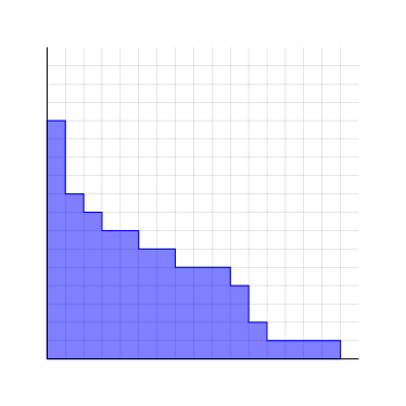
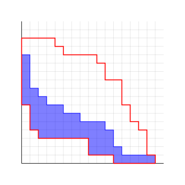
Figure 1: Unrestricted and restricted integer partitions.

3.1 The Biased Markov Chain

Let the state space $\Omega$ be the set of all Young diagrams restricted to lie in a region $R$. Young diagrams have a natural graded partial order via inclusion, where $\sigma\leq\rho$ if and only if $\sigma\subseteq\rho$, so the rank of a diagram $\sigma$ is $r(\sigma)=\lvert\sigma\rvert$. The following Markov chain $\mathcal{M}$ on the Hasse diagram of this partial order makes transitions that add or remove a square on the boundary of the diagram in each step according to the Metropolis-Hastings algorithm. Therefore the stationary distribution is a Boltzmann distribution parameterized by a bias value $\lambda$. Let $R$ be a region such that every partition restricted to this region has at most $\Delta$ neighboring configurations.

Biased Markov Chain on Integer Partitions $\mathcal{M}$

Starting at any Young diagram $\sigma_{0}\subseteq R$, repeat:

• Choose a neighbor $\rho$ of $\sigma_{t}$ uniformly at random with probability $1/2\Delta$.

• Set $\sigma_{t+1}=\rho$ with probability $\min(1,\lambda^{|\rho|-|\sigma_{t}|})$.

• With all remaining probability, set $\sigma_{t+1}=\sigma_{t}$.

The state space $\Omega$ is connected, because any configuration can eventually reach the minimum configuration $\sigma=\emptyset$ with positive probability. By construction, $\mathcal{M}$ is lazy (i.e., it is always possible that $\sigma_{t}=\sigma_{t+1}$), so it follows that $\mathcal{M}$ is an ergodic Markov chain, and hence has a unique stationary distribution $\pi$. Using the detailed balance equation for Markov chains [31], we see that $\pi(\sigma)=\lambda^{|\sigma|}$, for all $\sigma\in\Omega$.

This Markov chain can be used to efficiently approximate the number of partitions of $n$ restricted to $R$ within arbitrarily small specified relative error, because this problem is self-reducible [16]. Observe that we can run $\mathcal{M}$ restricted to $R$ polynomially many times and compute the mean height $m$ in the first column of the sampled Young diagrams. Then we use $\mathcal{M}$ to recursively approximate the number of partitions of $n-m$ restricted to the region

$$R^{\prime}=\{(x,y)\in R:1\leq x\text{ and }y\leq m\},$$

and return the product of $m$ and this approximation.

3.2 Sampling Using Balanced Bias

In the following general sampling theorem for restricted integer partitions, the mixing time of $\mathcal{M}$ must hold for all bias parameters $\lambda_{t}$.

Theorem 3.1.

Let $\tau=\tau(e^{-1})$ be the mixing time of $\mathcal{M}$ on the region $R$. We can uniformly sample partitions of $k$ restricted to a region $R$ in expected $O(\Delta\tau^{2})$ time.

Proof.

There is only one such partition when $k=0$ or $k=|R|$, so assume $k\in[|R|-1]$. By construction $|\Omega_{k+1}|/|\Omega_{k}|\leq\Delta$ for all fixed $k$, so $1\leq|\Omega_{i}|\leq\Delta^{i}$ for all $i\in\{0,1,\dots,|R|\}$. By Lemma 2.2 there exists a balanced bias $\lambda$, which we can identify adaptively in $O(\log(|R|))$ time with a binary search as we are sampling, since Boltzmann distributions increase monotonically with increasing $\lambda_{t}$. Therefore, we can generate Young diagrams restricted to $R$ with any fixed rank in expected $O(\Delta\tau^{2})$ steps of $\mathcal{M}$ by Theorem 2.2. ∎

If more is known about the number of elements at each rank or the geometry of $R$, then we can give better bounds on the runtime of this algorithm. For example, if $R$ is the region of a skew Young diagram (see Figure 1), a region contained between two Young diagrams, then we can adapt Levin and Peres’ mixing results about biased exclusion processes to this setting.

Theorem 3.2 ([23]).

Consider the biased exclusion process with bias $\beta=\beta_{n}=2p_{n}-1>0$ on the segment of length $2n$ and with $n$ particles. Set $\alpha=\sqrt{p_{n}/(1-p_{n})}$. For $\varepsilon>0$, if $n$ is large enough, then

$$\tau(\varepsilon)\leq\frac{4n}{\beta^{2}}\left[\log\left(\varepsilon^{-1}\right)+\log\left[\alpha\left(\frac{\alpha^{n}-1}{\alpha-1}\right)^{2}\right]\right].$$

Corollary 3.1.

If the region $R$ is a skew Young diagram contained in an $n\times n$ box, we can uniformly sample partitions of $k$ restricted to $R$ in expected $O(n^{16})$ time.

Proof.

The biased exclusion process on a segment of length $2n$ with $n$ particles is in bijection with $\mathcal{M}$ when the restricting region is an $n\times n$ box. The proof of Theorem 3.2 in [23] uses a path coupling argument that directly extends to and gives an upper bound for the mixing time of $\mathcal{M}$ when the region $R$ is a skew Young diagram, since the expected change in distance of two adjacent states in the more restricted setting can only decrease. Let $\lambda_{n,t}$ denote $\lambda_{t}$ in an instance of size $n$. We analyze the three cases $\lambda_{n,t}<1$, $\lambda_{n,t}=1$, and $\lambda_{n,t}>1$, and then bound the mixing time of $\mathcal{M}$ for all $\lambda_{n,t}$.

To prove the existence of a balanced bias using Lemma 2.2, observe that ${a_{\Omega,i}\leq p(i)\leq 2^{i}}$ for all $i\in\{0,1,\dots,n^{2}\}$. In the first case, assume $\lambda_{t,n}<1$. Then we have $t\in[n^{2}-1]$ since $|R|=n^{2}$. Translating $\mathcal{M}$ to the biased exclusion process,

$$p_{n,t}=\frac{1}{1+\lambda_{n,t}},$$

$$\beta_{n,t}=\frac{1-\lambda_{n,t}}{1+\lambda_{n,t}},$$

and

$$\alpha_{n}=\sqrt{\frac{1}{\lambda_{n,t}}}.$$

To use Theorem 3.2, we first prove $1/\beta_{n,t}^{2}\leq 10n^{4}$. To see this, observe that $t=n^{2}-1$ minimizes $\beta_{n,t}$, hence maximizes the desired quantity. Then

$$\lim_{n\rightarrow\infty}\left(\frac{1}{\beta_{n,n^{2}-1}}\right)^{2}=\frac{4n^{2}}{\log(2)^{2}}\leq 10n^{4}.$$

Next, since $a_{n,t}>1$, we have

$$\alpha_{n,t}\left(\frac{\alpha_{n,t}^{n}-1}{\alpha_{n,t}-1}\right)^{2}\leq~{}\alpha_{n,t}\left(n\alpha_{n,t}^{n}\right)^{2}~{}\leq~{}\frac{n^{2}}{\lambda_{n,t}^{n+1/2}}~{}\leq~{}n^{2}2^{n+1/2},$$

because $\lambda_{n,t}\geq 1/2$. Thus, $\tau(\varepsilon)=O(n^{5}(\log(\varepsilon^{-1})+n))$ for all $\lambda_{n,t}$ by Theorem 3.2.

In the unbiased case when $\lambda_{n,t}=1$, Wilson [35] proved that the mixing time of $\mathcal{M}$ is $\Theta(n^{3}\log(n/\varepsilon))$. In the third case, $\lambda_{t,n}>1$ so $t\in\{n^{2}+1,n^{2}+2,\dots,n^{4}\}$,

$$p_{n,t}=\frac{\lambda_{n,t}}{1+\lambda_{n,t}},$$

$$\beta_{n,t}=\frac{\lambda_{n,t}-1}{1+\lambda_{n,t}},$$

and

$$\alpha_{n,t}=\sqrt{\lambda_{n,t}}.$$

By similar analysis, $1/\beta_{n,t}^{2}\leq 10n^{4}$ and

$$\alpha_{n,t}\left(\frac{\alpha_{n,t}^{n}-1}{\alpha_{n,t}-1}\right)^{2}\leq~{}n^{2}\lambda_{n,t}^{n+1/2}~{}\leq~{}n^{2}\left(2^{n^{2}-1}\right)^{n+1/2},$$

since $\lambda_{n,t}\leq 2^{n^{2}-1}$. Thus $\tau(\varepsilon)=O(n^{5}(\log(\varepsilon^{-1})+n^{3}))$, so by Theorem 2.2 we can uniformly sample partitions of $k$ restricted to $R$ in expected $O(n^{16})$ time. ∎

3.3 Sampling Using Log-concavity

When more is known about the stationary distribution $\pi$, specifically the sequence $\{|\Omega_{i}|\}_{i=0}^{\infty}$, we can typically improve the bounds on the running time of our algorithm. In particular, we show that we can sample unrestricted integer partitions in expected $O(n^{9/4})$ time. Our primary techniques involve using a compressed representation of partitions and using log-concavity to show strong probability concentration around partitions of the desired size. These techniques extend to a variety of settings where log-concavity or probability concentration can be shown.

To sample integer partitions of $n$, we set the bias parameter $\lambda_{n}=p(n-1)/p(n)$ to force the stationary distribution to concentrate at $n$. The sequence $\{p(k)\}_{k=26}^{\infty}$ is log-concave [9, 27], so it follows that the sequence $\{p(k)\lambda_{n}^{k}\}_{k=26}^{\infty}$ is, too. Log-concave sequences of positive terms are unimodal, which implies that the mode of our stationary distribution is at $k=n$. Moreover, we show how log-concavity gives exponential decay on both sides of the mode, and hence strong concentration.

We now argue that we need only consider Young diagrams that lie under the curve $y=2n/x$ to sample partitions of $n$, as all Young diagrams with squares above that curve must have more than $2n$ squares total.

Proposition 3.1.

A Young diagram that lies under the curve $y=2n/x$ can be stored in $O(n^{1/2}\log(n))$ space.

Proof.

For any square in the Young diagram, both of its coordinates are not greater than $\sqrt{2n}$, for then it would lie above $y=2n/x$. We may record the height of each column and the width of each row in the range $\{0,1,\ldots,{\lfloor\sqrt{2n}\rfloor-1}\}$ to capture the position of every square in the diagram. Therefore, we can represent the diagram using exactly these $2\lfloor\sqrt{2n}\rfloor$ heights and widths. ∎

Using the compressed representation in the previous proposition, we see that there will not be more than $O(n^{1/2})$ possible transitions at any possible state, since our algorithms adds or removes at most one square on the upper boundary in each step. Note that we can adapt this technique in the general case for any region $R$ that lies under the curve $y=2n/x$.

Proposition 3.2.

There are at most $4\sqrt{2n}$ potential transitions for any Young diagram that lies under the curve $y=2n/x$.

Proof.

Observe that since the squares in any row or column must be connected, there are at most two valid moves in any particular row or column. Therefore, by Proposition 3.1, there are at most $4\lfloor\sqrt{2n}\rfloor$ possible transitions from any such Young diagram. ∎

We now shift our attention to bounding $\lambda_{n}$ and the consequences it has on both the mixing time of $\mathcal{M}$ and the concentration of $\pi$. Hardy and Ramanujan [14] gave the classical asymptotic formula for the partition numbers

$$p(n)\sim\frac{1}{4\sqrt{3}n}e^{\pi\sqrt{2n/3}},$$

and we use related bounds given in [9] for the following lemma. The proof is deferred to the next subsection.

Lemma 3.1.

For all $n\geq 30$, we have

$$1-\frac{2}{\sqrt{n}}~{}<~{}\lambda_{n}~{}<~{}1-\frac{1}{\sqrt{n}}.$$

Theorem 3.3.

The Markov chain $\mathcal{M}$ with bias $\lambda_{n}$ restricted to the region $R$ bounded by the curve $y=2n/x$ mixes in $O(n^{3/2}(\log(\varepsilon^{-1})+n^{1/2}))$.

Proof.

We modify Theorem 3.2 and its proof in [23]. In this biased exclusion process, $\lambda=\lambda_{n}$, $\beta=(1-\lambda)/(1+\lambda)$, and $\alpha=\sqrt{1/\lambda}$. By Proposition 3.2, there are at most $4\sqrt{2n}$ transitions from any state, so for $n$ large enough

$$\tau(\varepsilon)~{}\leq~{}\frac{8\sqrt{2n}}{\beta^{2}}\left[\log\left(\varepsilon^{-1}\right)+\log\left(\text{diam}\left(\Omega\right)\right)\right],$$

where $\text{diam}(\Omega)$ is the maximum length path between any two states, as defined in [24]. Therefore, we have $\text{diam}(\Omega)\leq|R|\alpha^{2n}$ and

$$|R|~{}\leq~{}2nH_{2n}~{}\leq~{}2n(\log(2n)+1),$$

so

$$\text{diam}(\Omega)~{}\leq~{}2n(\log(2n)+1)\alpha^{2n}~{}=~{}2n(\log(2n)+1)\lambda^{-n}.$$

By Lemma 3.1 and the bound $1+x\leq e^{x}$, for all $x\in\mathbb{R}$,

$$\log\left(\lambda^{-n}\right) \leq\log\left(\left(1+\frac{2}{\sqrt{n}-2}\right)^{n}\right)\leq 3\sqrt{n},$$

for $n$ sufficiently large. We have

$$\frac{1}{\beta}~{}\leq~{}2\sqrt{n}-1$$

by Lemma 3.1. Therefore, $\tau(\varepsilon)=O(n^{3/2}(\log(\varepsilon^{-1})+n^{1/2}))$. ∎

Another key observation we make to generate partitions of $n$ more efficiently is to salvage samples larger than $n$ instead of rejecting them, while preserving uniformity on the distribution $\Omega_{n}$. For any $k\geq 0$, consider the function $f_{k}:\Omega_{n}\rightarrow\Omega_{n+k}$ that maps a partition $\sigma=(\sigma_{1},\sigma_{2},\dots,\sigma_{m})$ to $f_{k}(\sigma)=(\sigma_{1}+k,\sigma_{2},\dots,\sigma_{m})$. Note that $\sigma_{1}\geq\sigma_{2}\geq\dots\geq\sigma_{m}$ since $\sigma$ is a Young diagram. Clearly $f_{k}$ is injective, so we can consider the inverse map $f^{-1}_{k}((\rho_{1},\rho_{2},\dots,\rho_{\ell}))$ that subtracts $k$ from $\rho_{1}$ if $\rho_{1}-k\geq\rho_{2}$, and is invalid otherwise. Then, define $g:\Omega_{\geq n}\rightarrow\Omega_{n}\cup\{0\}$ as

$$g((\rho_{1},\rho_{2},\dots,\rho_{\ell}))=\begin{cases}(\rho_{1}-k,\rho_{2},\dots,\rho_{\ell})&\text{if $\rho_{1}+\rho_{2}+\dots+\rho_{\ell}=n+k$ and $\rho_{1}-k\geq\rho_{2}$}\\ 0&\text{otherwise}.\end{cases}$$

The following lemma, whose proof is deferred to the next subsection, uses the log-concavity of the partition numbers to give a strong lower bound on the success of the map $g$.

Lemma 3.2.

Let $\sigma$ be a random Young diagram from the stationary distribution of $\mathcal{M}$, and let $g$ be the function defined above. Then for all $n$ sufficiently large,

$$\Pr[g(\sigma)\text{~{}generates a partition of }n]\geq\frac{1}{160n^{1/4}}.$$

Assembling the ideas in this section, we now formally present our Markov chain Monte Carlo algorithm for generating partitions of $n$ uniformly at random.

Algorithm for Sampling Integer Partitions

Repeat until success:

• Sample $\sigma\in\Omega$ using $\mathcal{M}$.

• If $n\leq\lvert\sigma\rvert\leq 2n$ and $g(\sigma)\neq 0$, return $g(\sigma)$.

Note that we restrict $\lvert\sigma\rvert\leq 2n$ instead of $\lvert\sigma\rvert\leq 2n\log(n)$ so that $g$ maps to $\Omega_{n}$ uniformly. All partitions of $2n$ are elements of $\Omega_{2n}$, but the same is not true for larger partitions since the bounding region $R$ is the curve $y=2n/x$. Lastly, recall that coupling from the past can be used efficiently in this setting to generate perfectly uniform samples, because the natural coupling is monotone and there is a single minimum and maximum configuration [13].

Theorem 3.4.

Our Markov chain Monte Carlo algorithm for generating a uniformly random partition of $n$ runs in expected $O(n^{9/4})$ time and $O(n^{1/2}\log(n))$ space.

Proof.

The proof directly follows from Proposition 3.1, Lemma 3.2, and Theorem 3.3. ∎

3.4 Proofs of Lemma 3.1 and Lemma 3.2

We prove Lemma 3.1 using bounds for $p(n)$ given in [9]. Let

$$\mu(n)=\mu_{n}=\frac{\pi\sqrt{24n-1}}{6},$$

$$\nu(n)=\nu_{n}=\frac{\sqrt{12}}{24n-1},$$

and

$$T(n)=\nu_{n}\left[\left(1-\frac{1}{\mu_{n}}\right)e^{\mu_{n}}+\frac{(-1)^{n}}{\sqrt{2}}e^{\mu_{n}/2}\right].$$

The function $T(n)$ is the sum of the three largest terms in the Hardy-Ramanujan formula, and the explicit error bounds in [9] that we use were first proved by Lehmer [22]. We only prove upper bounds in the following two proofs, as the lower bounds are proved similarly.

Lemma 3.3.

For all $n\geq 2$, we have

$$\left|p(n)-\nu_{n}\left(1-\frac{1}{\mu_{n}}\right)e^{\mu_{n}}\right|~{}<~{}1+e^{\mu_{n}/2}.$$

Proof.

By Lemma 2.3 and Proposition 2.4 in [9],

$$p(n)~{}<~{}T(n)+1+\frac{16}{\mu_{n}^{3}}e^{\mu_{n}/2}~{}<~{}\nu_{n}\left(1-\frac{1}{\mu_{n}}\right)e^{\mu}_{n}+1+e^{\mu_{n}/2}.\qed$$

Proof of Lemma 3.1..

By Lemma 3.3,

$$\lambda_{n}<\frac{1+e^{\mu_{n-1}/2}+\nu_{n-1}\left(1-\frac{1}{\mu_{n-1}}\right)e^{\mu_{n-1}}}{-\left(1+e^{\mu_{n}/2}\right)+\nu_{n}\left(1-\frac{1}{\mu_{n}}\right)e^{\mu_{n}}}=\frac{e^{\mu_{n-1}}}{e^{\mu_{n}}}\left(\frac{e^{-\mu_{n-1}}+e^{-\mu_{n-1}/2}+\nu_{n-1}\left(1-\frac{1}{\mu_{n-1}}\right)}{-\left(e^{-\mu_{n}}+e^{-\mu_{n}/2}\right)+\nu_{n}\left(1-\frac{1}{\mu_{n}}\right)}\right),$$

for all $n\geq 14$, because the lower bound for $p(n)$ is initially negative. We have

$$e^{-\mu_{n}}+e^{-\mu_{n}/2}<\frac{\nu_{n}}{n}\left(1-\frac{1}{\mu_{n}}\right),$$

for all $n\geq 65$, so it follows that

$$\lambda_{n}~{}<~{}\frac{e^{\mu_{n-1}}}{e^{\mu_{n}}}\left(\frac{\left(1+\frac{1}{n-1}\right)\nu_{n-1}\left(1-\frac{1}{\mu_{n-1}}\right)}{\left(1-\frac{1}{n}\right)\nu_{n}\left(1-\frac{1}{\mu_{n}}\right)}\right)=\frac{e^{\mu_{n-1}}}{e^{\mu_{n}}}\left(\frac{n}{n-1}\right)^{2}\left(\frac{\mu_{n}^{3}\left(\mu_{n-1}-1\right)}{\mu_{n-1}^{3}\left(\mu_{n}-1\right)}\right),$$

for all $n\geq 2$. Observe that $\mu_{n-1}-\mu_{n}<-\pi/\sqrt{6n}$ and

$$\frac{\mu_{n}^{3}\left(\mu_{n-1}-1\right)}{\mu_{n-1}^{3}\left(\mu_{n}-1\right)}~{}<~{}\frac{n}{n-1},$$

for all $n\geq 2$. Using $e^{x}\leq 1+x+x^{2}/2$, for all $x\leq 0$,

$$\lambda_{n}~{}<~{}\frac{e^{\mu_{n-1}}}{e^{\mu_{n}}}\left(\frac{n}{n-1}\right)^{3}<e^{-\frac{\pi}{\sqrt{6n}}}\left(\frac{n}{n-1}\right)^{3}\leq\left(1-\frac{\pi}{\sqrt{6n}}+\frac{\pi^{2}}{12n}\right)\left(\frac{n}{n-1}\right)^{3}<~{}1-\frac{1}{\sqrt{n}},$$

where the final inequality is true for all $n\geq 160$. When $30\leq n<160$, we verify the claim numerically. ∎

Now we prove Lemma 3.2 by showing that the truncation scheme $g(\sigma)$ succeeds with sufficient probability. By Hardy-Ramanujan formula, we have that for any constant $c>0$ and $n$ sufficiently large,

$$\frac{1-c}{4\sqrt{3}n}e^{\pi\sqrt{2n/3}}~{}\leq~{}p(n)~{}\leq~{}\frac{1+c}{4\sqrt{3}n}e^{\pi\sqrt{2n/3}}.$$

Letting $\lambda=\lambda_{n}$, the Hardy-Ramanujan formula implies that for all $n\geq 20$,

$$e^{-\pi k/\sqrt{6n}}~{}\leq~{}\lambda^{k}\leq e^{k/n-\pi k/\sqrt{6n}}.$$

Lemma 3.4.

Let $Z_{n}$ be the normalizing constant of the desired distribution. Then we have

$$Z_{n}<40n^{3/4}\lambda^{n}p(n),$$

for all $n$ sufficiently large.

Proof.

Clearly

$$Z_{n}\leq\sum_{k=0}^{\infty}p(k)\lambda^{k}.$$

We further know that $f(k)=p(k)\lambda^{k}$ is unimodal with a maximum at $k=n$. By the log-concavity of $\{f(k)\}_{k=26}^{\infty}$, we have

$$\frac{f(n+k)}{f(n)}\geq\frac{f(n+2k)}{f(n+k)}$$

and

$$\frac{f(n-k)}{f(n)}\geq\frac{f(n-2k)}{f(n-k)},$$

for all $k\geq 1$. Therefore, we can bound $Z_{n}$ as

$$Z_{n}\leq kf(n)\left(\frac{1}{1-\frac{f(n+k)}{f(n)}}+\frac{1}{1-\frac{f(n-k)}{f(n)}}\right),$$

for any $k\geq 1$. Specifically, if both $f(n+k)/f(n)$ and $f(n-k)/f(n)$ are at most some fixed constant less than $1$, then $Z_{n}=O(kf(n))$. Using the bounds above,

$$f(k)~{}=~{}p(k)\lambda^{k}~{}\leq~{}\frac{1+c}{4\sqrt{3}k}e^{k/n-\pi\left(k-2\sqrt{kn}\right)/\sqrt{6n}}~{}=~{}\frac{1+c}{4\sqrt{3}k}e^{k/n-\pi\left(\sqrt{k}-\sqrt{n}\right)^{2}/\sqrt{6n}+\pi\sqrt{n/6}}.$$

Letting $n+k=(\sqrt{n}+n^{1/4})^{2}$, for $n$ large enough,

$$f\left(\left(\sqrt{n}+n^{1/4}\right)^{2}\right)~{}\leq~{}\frac{1+c}{4\sqrt{3}n}e^{1.1-\pi/\sqrt{6}+\pi\sqrt{n/6}}.$$

We can then bound the density value at $(\sqrt{n}+n^{1/4})^{2}$ relative to the maximum by

$$\frac{f\left(\left(\sqrt{n}+n^{1/4}\right)^{2}\right)}{f(n)}~{}\leq~{}\frac{\frac{1+c}{4\sqrt{3}n}e^{1.1-\pi/\sqrt{6}+\pi\sqrt{n/6}}}{\frac{1-c}{4\sqrt{3}n}e^{\pi\sqrt{2n/3}-\pi\sqrt{n/6}}}~{}=~{}\frac{1+c}{1-c}e^{1.1-\pi/\sqrt{6}}.$$

Taking $c\leq 0.01$, we have

$$\frac{f\left(\left(\sqrt{n}+n^{1/4}\right)^{2}\right)}{f(n)}~{}\leq~{}\frac{1.01}{0.99}e^{1.1-\frac{\pi}{\sqrt{6}}}~{}<~{}0.85.$$

Similarly, for $n$ sufficiently large,

$$\frac{f\left(\left(\sqrt{n}-n^{1/4}\right)^{2}\right)}{f(n)}~{}<~{}0.85.$$

Therefore, we have $Z_{n}<40n^{3/4}\lambda^{n}p(n)$ using the fact that $k\leq 3n^{3/4}$. ∎

Proof of Lemma 3.2..

We use Lemma 3.4 and Lemma 3.1 to bound the probability that $g(\sigma)$ generates a partition of $n$ successfully. Therefore, we have

$$\Pr[g(\sigma)\text{ generates a partition of }n] =\sum_{k=0}^{n}\frac{\lambda^{n+k}p(n)}{Z_{n}}$$

$$\geq\frac{1}{40n^{3/4}}\sum_{k=0}^{n}\lambda^{k}$$

$$\geq\frac{1}{40n^{3/4}}\sum_{k=0}^{n}\left(1-\frac{2}{\sqrt{n}}\right)^{k}$$

$$=\frac{1}{40n^{3/4}}\cdot\frac{\sqrt{n}}{2}\left(1-\left(1-\frac{2}{\sqrt{n}}\right)^{n+1}\right)$$

$$\geq\frac{1}{160n^{1/4}}.\qed$$

4 Sampling in Other Graded Posets

We demonstrate the versatility of using a Markov chain on the Hasse diagram of a graded poset to sample elements of fixed rank. When this chain is rapidly mixing for all $\lambda_{t}$ with ${t\in[R^{2}]}$, we can apply Boltzmann sampling and Theorem 2.2 to generate approximately uniform samples in polynomial time. Similar to region-restricted integer partitions, analogous notions of self-reducibility apply to restricted families of permutations and lozenge tilings, so there exist fully polynomial-time approximation schemes for these enumerations problems because we can efficiently sample elements of a given rank from their respective posets [16].

4.1 Permutations with Fixed Rank

In the first case, we consider permutations of $n$ elements with a fixed number of inversions. The Hasse diagram in this setting connects permutations that differ by one adjacent transposition. This partial order is in bijection with the weak Bruhat order on the symmetric group. In the unbiased case ($\lambda=1$), the nearest neighbor Markov chain mixes in time $\Theta(n^{3}\log(n))$ [35]. With constant bias the chain is known to converge in time $\Theta(n^{2})$ [5, 13]. The number of permutations of $n$ with $k$ inversions is known to be log-concave in $k$, so standard Boltzmann sampling techniques can be used. However, using our balanced bias method, we avoid the need for bounds on the growth of inversion numbers in restricted settings, such as permutations where at least $i$ of the first $j$ elements are in the first half of the permutation. Figure 2 illustrates the distribution of inversions of random permutations in $S_{100}$ sampled from various ranks of the inversion poset as Rothe diagrams [21].

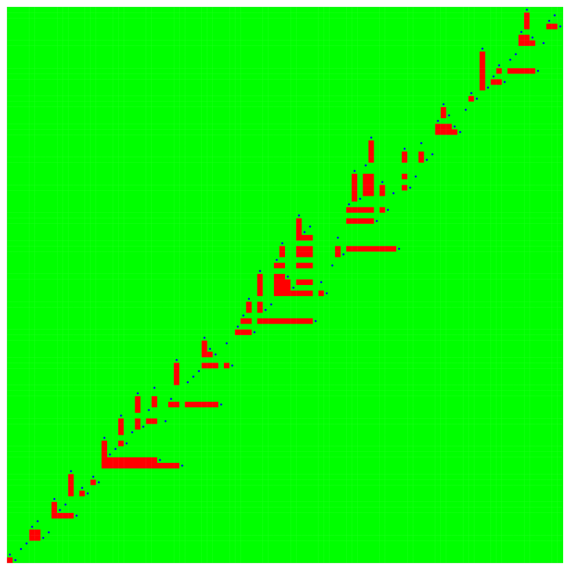
(a)

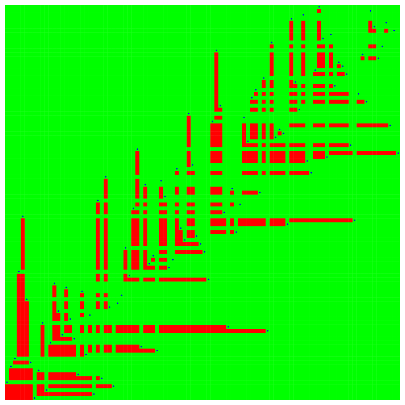
(b)

(c)

(d)

(e)

(f)

Figure 2: Random permutations with (a) 5, (b) 20, (c) 40, (d) 60, (e) 80, (f) 95 percent of $\binom{100}{2}$ inversions.

4.2 Lozenge Tilings with Fixed Average Height

Lozenge tilings are tilings of a triangular lattice region with pairs of equilateral triangles that share an edge. There is a well-studied height function that maps hexagonal lozenge tilings bijectively to plane partitions lying in an $n\times n\times n$ box (see, e.g., [25]), and it follows that lozenge tilings with a fixed average height of $k$ are precisely the plane partitions with volume $k$. The Markov chain that adds or removes single cubes on the surface of the plane partition (corresponding to rotating three nested lozenges 180 degrees) is known to mix rapidly in the unbiased case. Caputo et al. [7] studied the biased version of this chain with a preference toward removing cubes, and showed that this chain converges in $O(n^{3})$ time. Applying the balanced bias method, we can use Boltzmann sampling to generate random lozenge tilings with any target average height in polynomial time, as shown in Figure 3.

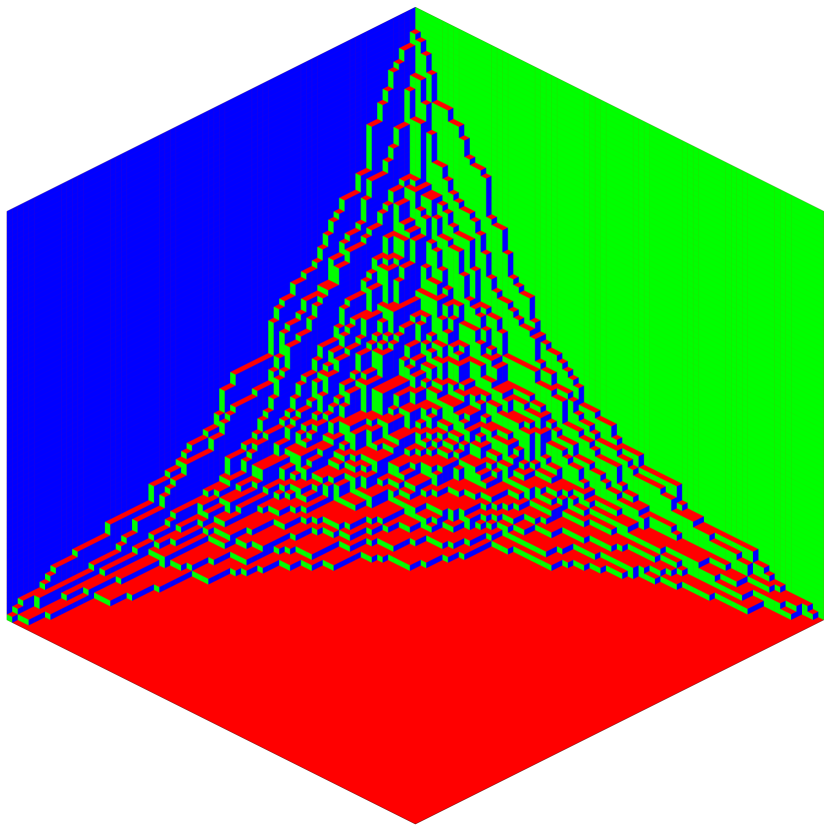
(a)

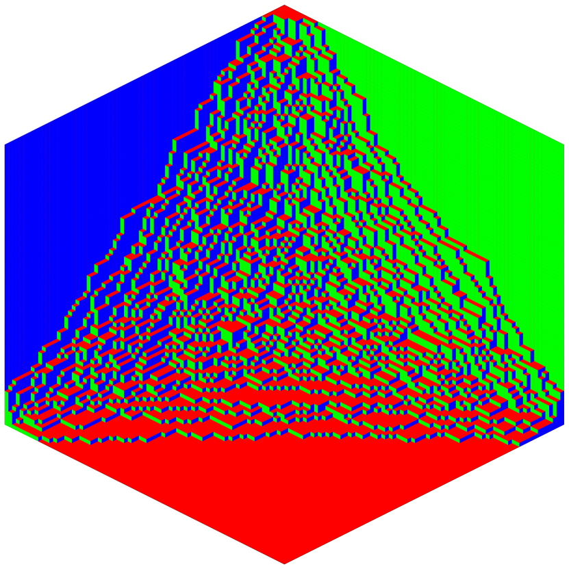
(b)

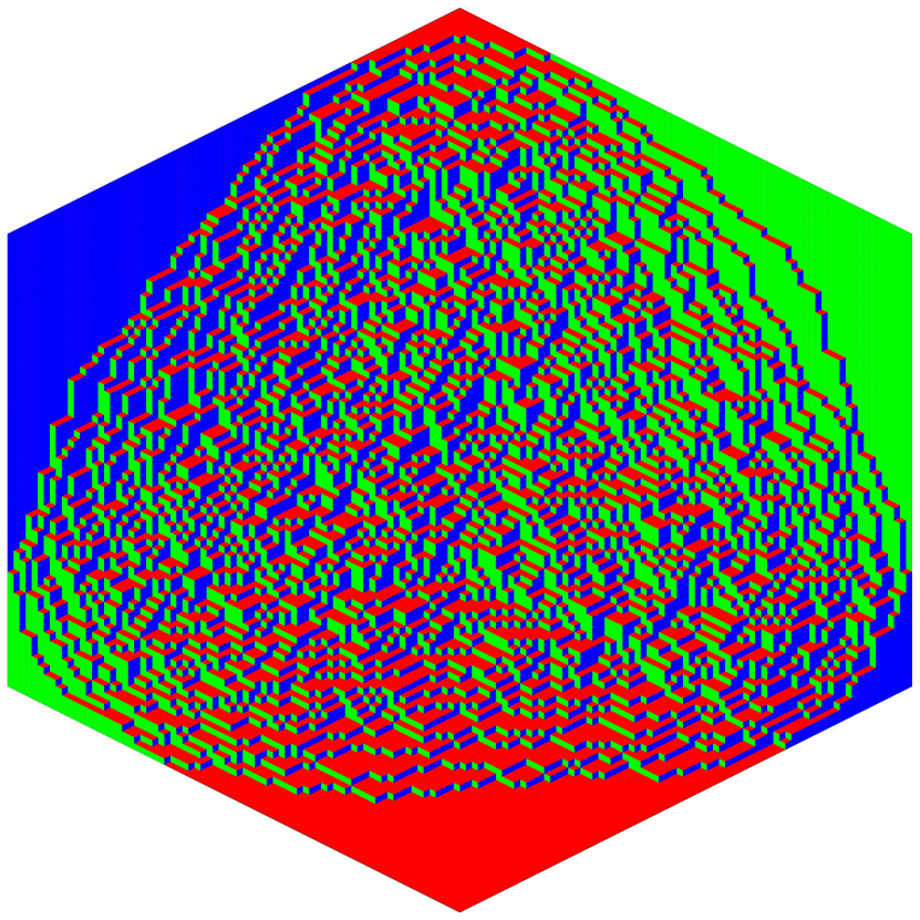
(c)

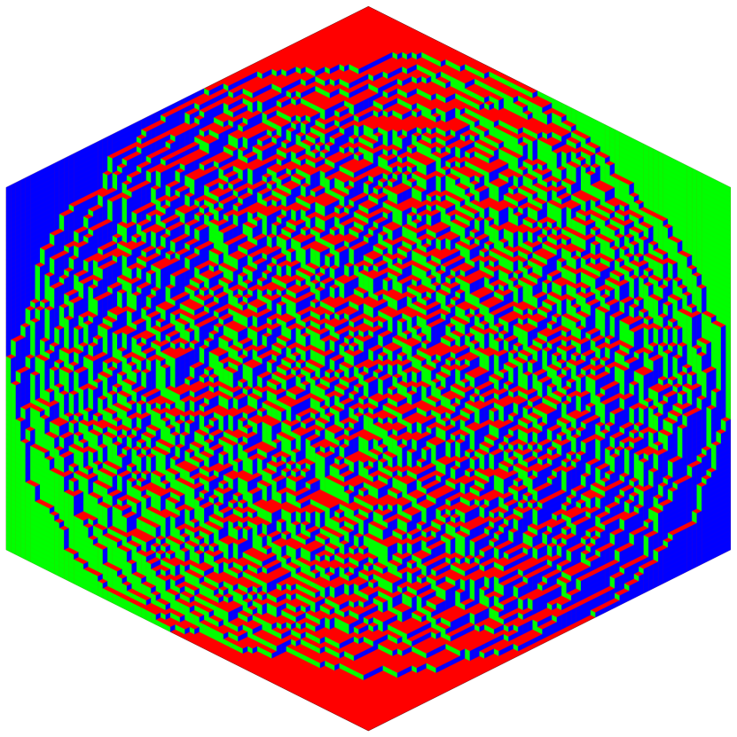
(d)

Figure 3: Random lozenge tilings with average height (a) 5, (b) 15, (c) 35, (d) 50 percent of $75^{3}$.

References

- [1] D. Aldous. Deterministic and stochastic models for coalescence (aggregation and coagulation): a review of the mean-field theory for probabilists. Bernoulli, 5(1):3–48, 1999.
- [2] G. E. Andrews. The Theory of Partitions. Cambridge mathematical library. Cambridge University Press, 1998.
- [3] R. Arratia and S. DeSalvo. Probabilistic divide-and-conquer: a new exact simulation method, with integer partitions as an example. Combinatorics, Probability and Computing, 25(3):324–351, 2016.
- [4] A. Ayyer, J. Bouttier, S. Corteel, and F. Nunzi. Multivariate juggling probabilities. Electronic Journal of Probability, 20(5):1–29, 2014.
- [5] I. Benjamini, N. Berger, C. Hoffman, and E. Mossel. Mixing times of the biased card shuffling and the asymmetric exclusion process. Transactions of the American Mathematical Society, 357(8):3013–3029, 2005.
- [6] N. Berestycki and J. Pitman. Gibbs distributions for random partitions generated by a fragmentation process. Journal of Statistical Physics, 127:381–418, 2007.
- [7] P. Caputo, F. Martinelli, and F. L. Toninelli. Convergence to equilibrium of biased plane partitions. Random Structures & Algorithms, 39(1):83–114, 2011.
- [8] A. Comtet, S. N. Majumdar, and S. Ouvry. Integer partitions and exclusion statistics. Journal of Physics A: Mathematical and Theoretical, 40(37):11255–11269, 2007.
- [9] S. DeSalvo and I. Pak. Log-concavity of the partition function. The Ramanujan Journal, 38(1):61–73, 2014.
- [10] P. Duchon, P. Flajolet, G. Louchard, and G. Shaeffer. Boltzmann samplers for the random generation of combinatorial structures. Combinatorics, Probability and Computing, 13(4–5):577–625, 2004.
- [11] P. Flajolet, É. Fusy, and C. Pivoteau. Boltzmann sampling of unlabelled structures. In Proceedings of the Fourth Workshop on Analytic Algorithmics and Combinatorics (ANALCO), pages 201–211, 2007.
- [12] B. Fristedt. The structure of random partitions of large integers. Transactions of the American Mathematical Society, 337(2):703–735, 1993.
- [13] S. Greenberg, A. Pascoe, and D. Randall. Sampling biased lattice configurations using exponential metrics. In Proceedings of the Twentieth Annual ACM-SIAM Symposium on Discrete Algorithms (SODA), pages 76–85, 2009.
- [14] G. H. Hardy and S. Ramanujan. Asymptotic formulae in combinatory analysis. Proceedings of the London Mathematical Society, 17:75–115, 1918.
- [15] G. D. James and A. Kerber. The representation theory of the symmetric group. Encyclopedia of Mathematics and its Applications. Cambridge University Press, 1984.
- [16] M. Jerrum. Counting, Sampling and Integrating: Algorithms and Complexity. Lectures in Mathematics. ETH Zürich. Birkhäuser Basel, 2003.
- [17] M. Jerrum and A. Sinclair. Approximate counting, uniform generation and rapidly mixing Markov chains. Information and Computation, 82:93–133, 1989.
- [18] M. Jerrum and A. Sinclair. The Markov chain Monte Carlo method: an approach to approximate counting and integration. In D. S. Hochbaum, editor, Approximation Algorithms for NP-hard Problems, pages 482–520. PWS Publishing, 1997.
- [19] M. R. Jerrum, A. J. Sinclair, and E. Vigoda. A polynomial-time approximation algorithm for the permanent of a matrix with nonnegative entries. Journal of the ACM, 41:671–697, 2006.
- [20] R. Kenyon and A. Okounkov. Limit shapes and the complex Burgers equation. Acta Mathematica, 199:263–302, 2007.
- [21] A. Kerber. Applied Finite Group Actions. Algorithms and Combinatorics. Springer Berlin Heidelberg, 2013.
- [22] D. H. Lehmer. On the series for the partition function. Transactions of the American Mathematical Society, 43(2):271–295, 1938.
- [23] D. Levin and Y. Peres. Mixing of the exclusion process with small bias. Preprint available at https://arxiv.org/abs/1608.03633, 2016.
- [24] D. Levin, Y. Peres, and E. Wilmer. Markov chains and mixing times. American Mathematical Society, 1st edition, 2008.
- [25] M. Luby, D. Randall, and A. J. Sinclair. Markov chain algorithms for planar lattice structures. SIAM Journal on Computing, 31:167–192, 2001.
- [26] N. Metropolis, A. W. Rosenbluth, M. N. Rosenbluth, A. H. Teller, and E. Teller. Equation of State Calculations by Fast Computing Machines. The Journal of Chemical Physics, 21(6):1087–1092, 1953.
- [27] J. L. Nicolas. Sur les entiers pour lesquels il y a beaucoup de groupes abéliens d’ordre . Annales de l’institut Fourier, 28(4):1–16, 1978.
- [28] A. Nijenhuis and H. S. Wilf. Combinatorial algorithms. Academic Press, 1978.
- [29] A. Okounkov. Symmetric Functions and Random Partitions, pages 223–252. Springer Netherlands, Dordrecht, 2002.
- [30] J. G. Propp and D. B. Wilson. Exact sampling with coupled markov chains and applications to statistical mechanics. Random Structures & Algorithms, 9(1–2):223–252, 1996.
- [31] D. Randall. Mixing. In 44th Symposium on Foundations of Computer Science (FOCS), pages 4–15, 2003.
- [32] A. Sinclair. Improved bounds for mixing rates of Markov chains and multicommodity flow. Combinatorics, Probability and Computing, 1:351–370, 1992.
- [33] A. Sinclair. Algorithms for random generation and counting. Progress in theoretical computer science. Birkhäuser, 1993.
- [34] M. Squire. Efficient generation of integer partitions. Unpublished manuscript, 1993.
- [35] D. B. Wilson. Mixing times of lozenge tiling and card shuffling Markov chains. The Annals of Applied Probability, 14(1):274–325, 2004.